simple sys- tems - mcgill university · tems which are the basic building blocks of...
TRANSCRIPT

To summarize, the main conclusion so far is:
The existence and (essential) uniqueness of entropy is
equivalent to the (very natural) assumptions A1-A6
about the relation of adiabatic accessibility plus the
comparison property, CP.
However, CP is not at all self evident, as can be seen
by considering systems where “rubbing” and “thermal
equilibration” are the only adiabatical operations.
1

An essential part of our analysis is a derivation of CP
from additional assumptions about SIMPLE SYS-
TEMS which are the basic building blocks of ther-
modynamics. At the same time we make contact
with the traditional concepts of thermodynamic like
pressure and temperature.
2

The states of simple systems are described by one
energy coordinate, the internal energy, U , (the First
Law enters here) and one or more work coordinates,
like the volume V . (Note: U, V are fundamental (not
(P, V ) or (P, T ), etc.)
Thus the state space of a simple system is no longer
just an abstract set but a concrete subset of an R1+n.
3
FIRST LAW OF THERMODYNAMICS
If the state of a system is changed in an adiabatic
process, i.e., such that the only net effect in the sur-
roundings is the raising or lowering of a weight, then
the energy delivered or received by the weight depends
only on the initial and the final state of the system.
The internal energy U(X) is defined by measuring the
energy change with respect to some reference state
X0 in a process that either takes X0→ X or X → X0.4

We now assume (A1)-(A6), and for simple systems in
addition the following
SIMPLE SYSTEM AXIOMS
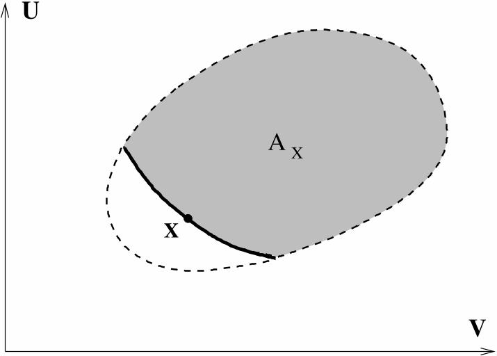
S1. Convex Combination:
((1− λ)X,λY ) ≺ (1− λ)X + λY.
(This implies that the forward sector
AX = {Y ∈ Γ : X ≺ Y }
is a convex set.)5
U
V
X
XA

S2. Existence of irreversible processes: For every
X there is a Y with X ≺≺ Y .
Given the other axioms this is equivalent to Caratheodory’s
principle: In every neighbourhood of every X ∈ Γ there
is a Z ∈ Γ with X 6≺ Z. It also implies that every X
lies on the boundary of its forward sector.
6
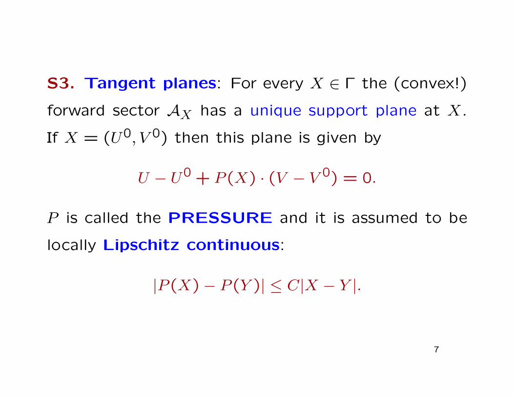
S3. Tangent planes: For every X ∈ Γ the (convex!)
forward sector AX has a unique support plane at X.
If X = (U0, V 0) then this plane is given by
U − U0 + P (X) · (V − V 0) = 0.
P is called the PRESSURE and it is assumed to be
locally Lipschitz continuous:
|P (X)− P (Y )| ≤ C|X − Y |.
7
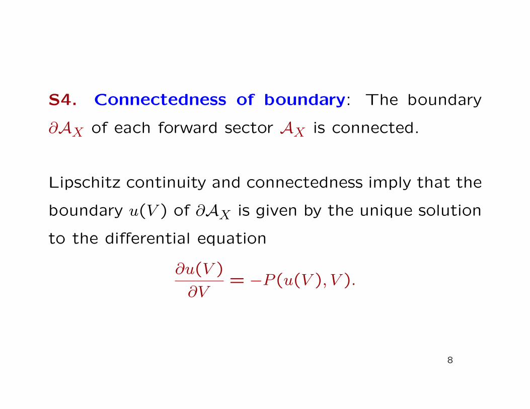
S4. Connectedness of boundary: The boundary
∂AX of each forward sector AX is connected.
Lipschitz continuity and connectedness imply that the
boundary u(V ) of ∂AX is given by the unique solution
to the differential equation
∂u(V )
∂V= −P (u(V ), V ).
8

From these assumptions the main theorem about sim-
ple systems can be proved:
THEOREM 3 (Comparability for simple systems)
If X and Y are two states of a simple system, Γ, then
either X ≺ Y , or Y ≺ X. Moreover,
X ∼A Y ⇐⇒ Y ∈ ∂AX ⇐⇒ X ∈ ∂AY
9

Y’X’
X’’Y’’
U
V
U
V
right
wrong
Y
Z
X
Y
X
16

To define S, however, comparability of the states in Γ
is not enough. We need more, namely comparability
on (1− λ)Γ× λΓ for all λ ∈ [0,1]!
For this we shall appeal to THERMAL CONTACT
established for instance by connecting the systems via
a copper thread. This produces a new simple system
out of two others,. Applying the previous results to
this system will then imply comparability also for the
product of the two systems.
10
We now formalize this idea by making four assump-
tions.
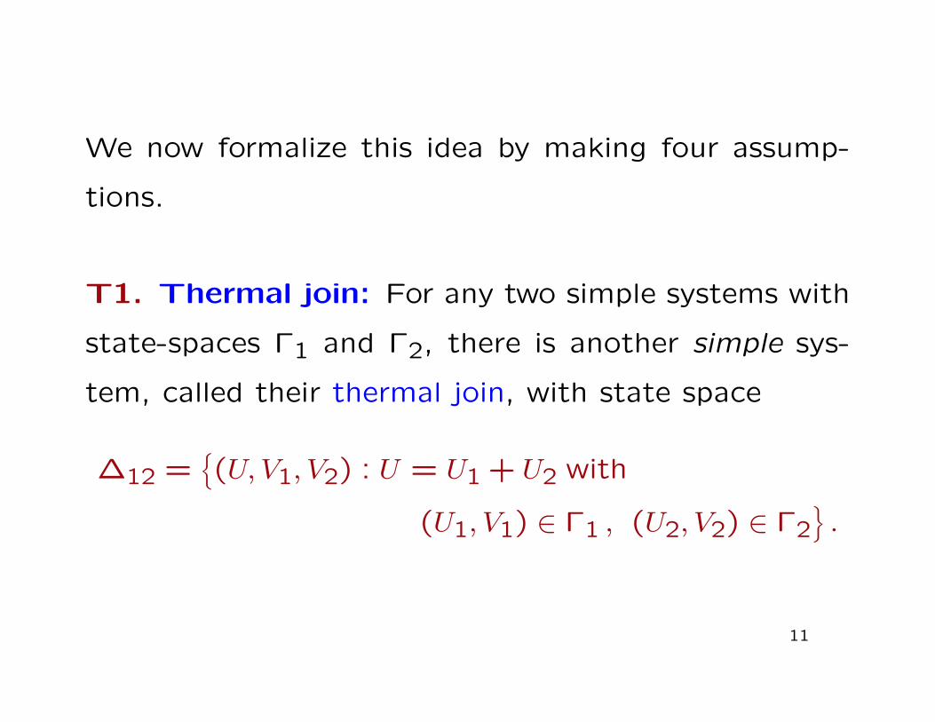
T1. Thermal join: For any two simple systems with
state-spaces Γ1 and Γ2, there is another simple sys-
tem, called their thermal join, with state space
∆12 ={(U, V1, V2) : U = U1 + U2 with
(U1, V1) ∈ Γ1 , (U2, V2) ∈ Γ2}.
11
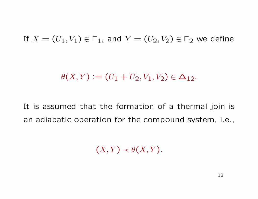
If X = (U1, V1) ∈ Γ1, and Y = (U2, V2) ∈ Γ2 we define
θ(X,Y ) := (U1 + U2, V1, V2) ∈∆12.
It is assumed that the formation of a thermal join is
an adiabatic operation for the compound system, i.e.,
(X,Y ) ≺ θ(X,Y ).
12
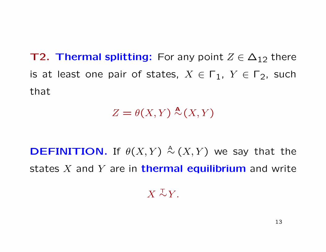
T2. Thermal splitting: For any point Z ∈∆12 there
is at least one pair of states, X ∈ Γ1, Y ∈ Γ2, such
that
Z = θ(X,Y ) ∼A (X,Y )
DEFINITION. If θ(X,Y ) ∼A (X,Y ) we say that the
states X and Y are in thermal equilibrium and write
X ∼T Y .
13

S1 and S2 together say that for each choice of the
individual work coordinates there is a way to divide
up the energy U between the two systems in a sta-
ble manner. S2 is the stability statement, for it says
that joining is reversible, i.e., once the equilibrium has
been established, one can cut the copper thread and
retrieve the two systems back again, but with a special
partition of the energies.
T3. Zeroth law: X ∼T Y and Y ∼T Z ⇒ X ∼T Z.
14

The equivalence classes w.r.t. the relation ∼T are called
isotherms.
T4. Transversality: If Γ is the state space of a
simple system and if X ∈ Γ, then there exist states
X0 ∼T X1 with X0 ≺≺ X ≺≺ X1.
Intuitively this says that adiabats and isotherms do
not coincide.
15

U
V
X
X
0
1
1
X0
Y Y
Y

With these axioms one establishes comparison for com-
pound systems, which is needed for the construction
of S and the consistent adjustment of entropy units
for different systems to ensure additivity.
The key point is that the states ((1− λ)X0, λX1) and
X ∼A ((1 − λ)X,λX) can be regarded as states of the
same simple system (the thermal join of (1− λ)Γ and
λΓ) and are hence comparable, by Theorem 2.
16

THEOREM 4 (Thermal contact implies CP.) The
comparison property holds for arbitrary scaled prod-
ucts of simple systems. Hence the relation ≺ in such
state spaces is characterized by an additive and exten-
sive entropy, S. The entropy is unique up to an overall
multiplicative constant and one additive constant for
each ‘basic’ simple system.
Moreover, the entropy is a concave function of the en-
ergy and work coordinates (by S1), and it is nowhere
locally constant (by S2).17

The uniqueness is very important! It means that en-
tropy can be determined in the usual way from heat
capacities, compressibilities etc by integration:
S(X)− S(X0) =∫X0→X
dU + PdV
T.
But first we must define T !
18

THEOREM 5 (Entropy defines temperature.) The
entropy, S, is a continuously differentiable function on
the state space of a simple system. If the function T
is defined by
1/T =(∂S
∂U
)V
then T characterizes the relation ∼T in the sense that
X ∼T Y ⇔ T (X) = T (Y ).
19
Moreover, if two systems are brought into thermal
contact with fixed work coordinates, then energy flows
from the system with higher value T to the system
with lower value of T .
REMARK While adiabats, i.e., the level sets of S,
are convex hypersurfaces, the isotherms can be much
more complicated.
20

U
V
S
L
G T1
T2
T3L&G
S&L
S&G
18

MIXTURES AND CHEMICAL REACTIONS
The problem is to choose the entropy constants for
different chemical compounds and mixtures in a con-
sistent way.
Usual approach: appeal to ‘semipermeable membranes’
that don’t really exist in nature.
Can be avoided!
21

But need one more axiom:
M1 (Absence of sinks): If Γ and Γ′ are state spaces
such that X ≺ Y for some X ∈ Γ, Y ∈ Γ′, then Z ≺W
for some Z ∈ Γ′, W ∈ Γ.
THEOREM 6. (Universal entropy.) The additive
entropy constants of all systems can be calibrated in
such a way that the entropy is additive and extensive,
and X ≺ Y implies S(X) ≤ S(Y ), even when X and Y
do not belong to the same state space.22
CONCLUSIONS
A line of thought that can be traced back to C.
Caratheodory, P.-T. Landsberg, H.-A. Buchdahl, G.
Falk, P. Jung and R. Giles has led to an axiomatic
foundation for thermodynamics.
What, if anything, has been gained compared to the
usual approaches involving concepts like ’quasi-static
processes’, ’heat’ and ’Carnot machines’ on the one
hand and statistical mechanics on the other hand?23
1) It is not necessary to introduce intuitive concepts
like ’heat’, ’hot’, ’cold’, ’quasi-static processes’ nor
’semipermeable membranes’ as primitive concepts. Also
’temperature’ becomes a derived concept.
2) In order to define entropy, there is no need for
special machines and processes on the empirical side,
and there is no need for assumptions about models on
the statistical mechanical side. Entropy is seen as a
codification of possible state changes that can be ac-
complished without changing the rest of the universe
in any way except for moving a weight.24
Just as energy conservation was eventually seen to be
a consequence of time translation invariance, in like
manner entropy can be seen to be a consequence of
some simple properties of the list of state pairs related
by adiabatic accessibility.
If the second law can be demystified, so much the
better. If it can be seen to be a consequence of simple,
plausible notions then, as Einstein said, it cannot be
overthrown.
25

SOME APPLICATIONS OF ENTROPY
1. THE CARNOT LIMIT ON EFFICIENCY
Define a thermal reservoir to by a system with fixed
work coordinates and so large that its temperature
can be taken to be independent of the energy.
If the energy of a reservoir changes by ∆Ures, the
entropy change is therefore
∆Sres =∆Ures
Tres26
Consider now two reservoirs with temperatures
Th > T` > 0 and a machine that couples to the reser-
voirs in a cyclic process, delivering the work (mechan-
ical energy) W in each cycle.
By the First Law
∆Uh + ∆U` +W = 0
and by the Second Law
∆Sh + ∆S` ≥ 027

i.e.∆UhTh
+∆U`T`≥ 0.
Since ∆Uh < 0 and T` > 0 this implies
∆U`∆Uh
≤ −T`Th.
The efficiency is defined as
η =W
−∆Uh=
1 +∆U`∆Uh
and we obtain
η ≤ ηC :=
1−T`Th
.28

2. AVAILABLE ENERGY (EXERGY)
Consider the surrounding of a system as a reservoir
of temperature T0. How much work can be extracted
from system+surrounding if the system ends up at
temperature T0 with energy U0 and entropy S0?
First law:
∆U + ∆Ures +W = 0.
Second law:
∆S + ∆Sres ≥ 0.
29

Now
∆Sres =∆Ures
T0
so the 1st and 2nd laws imply
∆S −∆U −W
T0≥ 0,
or, with ∆U = U0 − U , ∆S = S0 − S,
W ≤ (U − U0)− T0(S − S0) =: Φ.
The quantity Φ is called available energy or exergy.
30

REMARKS
1. Φ depends both on the system and the surround-
ing.
2. The energy difference U −U0 can have either sign,
but Φ is always nonnegative! (By concavity of en-
tropy.)
3. In the example of the iceberg in the Gulf Stream,
U−U0 < 0, but Φ is positive because the loss of energy
is outweighed by the negative T0(S − S0).
31
3. EQUATIONS OF STATE
The thermal equation(s) of state
P = P (T, V )
and the caloric equation of state
U = U(T, V )
describe the properties of a simple thermodynamic
system.
32
The latter gives the heat capacity at constant vol-
ume
CV =(∂U
∂T
)V.
The former gives the isothermal compressibility
κT = −1
V
(∂V
∂P
)T
and the thermal expansion coefficient
αV =1
V
(∂V
∂T
)V.
33
Both equations of state follow from the fundamental
equation
dS =1
TdU +
P
TdV
by differentiation:
1
T=
(∂S
∂U
)V⇒ U = U(T, V )
P
T=
(∂S
∂V
)U⇒ P = U(T, V ).
34

We say that S as a function of its natural variables
(U, V ) is a thermodynamic potential.
It is a remarkable consequence of the fundamental
equation that the equations of state are not indepen-
dent.
Their connection is derived as follows:
35
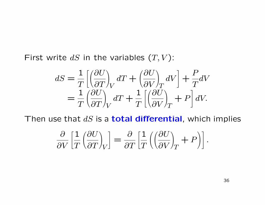
First write dS in the variables (T, V ):
dS =1
T
[(∂U
∂T
)VdT +
(∂U
∂V
)TdV
]+P
TdV
=1
T
(∂U
∂T
)VdT +
1
T
[(∂U
∂V
)T
+ P
]dV.
Then use that dS is a total differential, which implies
∂
∂V
[1
T
(∂U
∂T
)V
]=
∂
∂T
[1
T
((∂U
∂V
)T
+ P
)].
36
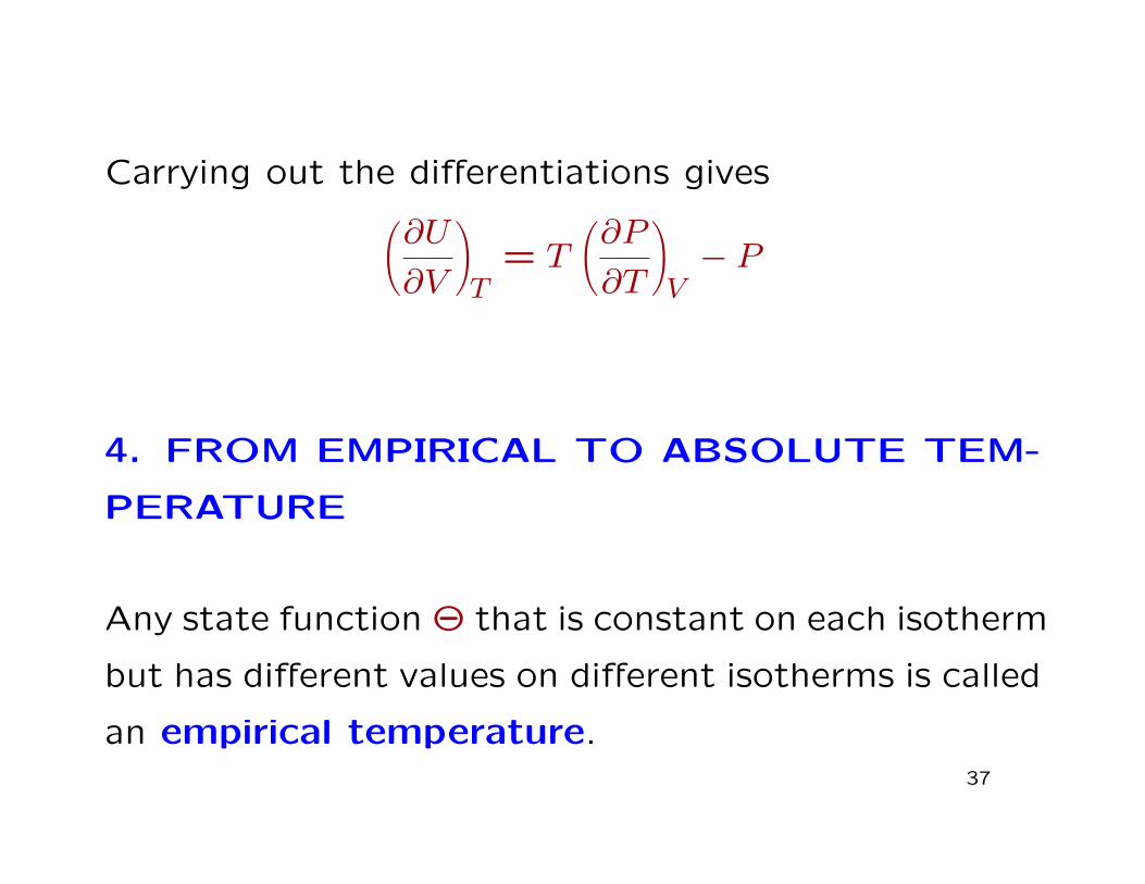
Carrying out the differentiations gives(∂U
∂V
)T
= T
(∂P
∂T
)V− P
4. FROM EMPIRICAL TO ABSOLUTE TEM-
PERATURE
Any state function Θ that is constant on each isotherm
but has different values on different isotherms is called
an empirical temperature.37

Thus Θ is a strictly monotone function of T alone;
we assume it to be differentiable.
The connection between the caloric and thermal equa-
tions of state allows us to compute the inverse func-
tion T = T (Θ) from directly measurable quantities.
First note that by the chain rule(∂P
∂T
)V
=(∂P
∂Θ
)V
dΘ
dT.
38

Inserted into the connection between the caloric and
thermal equations of state gives a differential equation
for T = T (Θ):(∂U
∂V
)Θ
= T
(∂P
∂Θ
)V
dΘ
dT− P.
that can be rewritten
1
T
dT
dΘ=
(∂P∂Θ
)V
P +(∂U∂V
)Θ
.
39
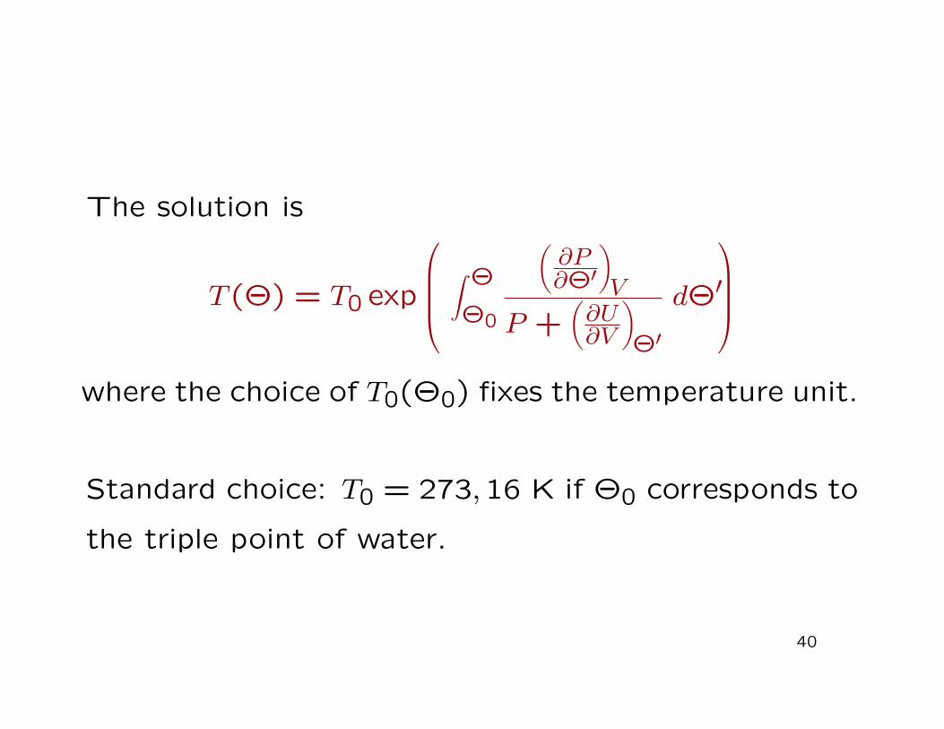
The solution is
T (Θ) = T0 exp
∫ Θ
Θ0
(∂P∂Θ′
)V
P +(∂U∂V
)Θ′
dΘ′
where the choice of T0(Θ0) fixes the temperature unit.
Standard choice: T0 = 273,16 K if Θ0 corresponds to
the triple point of water.
40
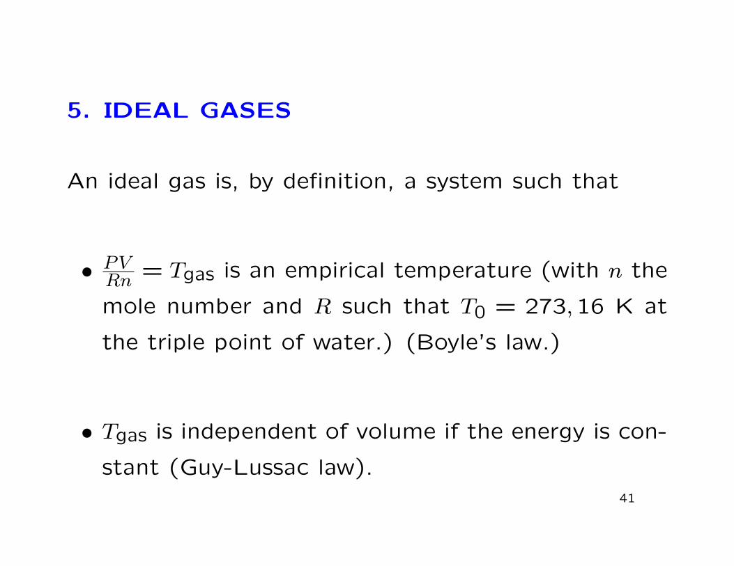
5. IDEAL GASES
An ideal gas is, by definition, a system such that
• PVRn = Tgas is an empirical temperature (with n the
mole number and R such that T0 = 273,16 K at
the triple point of water.) (Boyle’s law.)
• Tgas is independent of volume if the energy is con-
stant (Guy-Lussac law).41
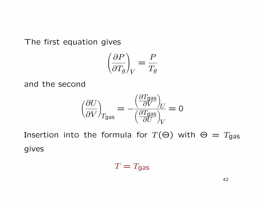
The first equation gives ∂P∂Tg
V
=P
Tg
and the second
(∂U
∂V
)Tgas
= −
(∂Tgas∂V
)U(
∂Tgas∂U
)V
= 0
Insertion into the formula for T (Θ) with Θ = Tgas
gives
T = Tgas
42

6. COMPUTATION AND MEASUREMENT OF
ENTROPY
In the variables (T, V ) the fundamental equation is
dS =1
T
(∂U
∂T
)VdT +
1
T
[(∂U
∂V
)T
+ P
]dV.
Using the connection between the caloric and ther-
mal equations of state and the definition of the heat
capacity CV we can write this as
dS =CVTdT +
(∂P
∂T
)VdV.
43

This form is very useful for the determination of S in
practice by integration along a suitable path. Heat
capacities and (∂P/∂T )V are also directly measurable.
For an ideal gas with a constant heat capacity we
obtain as an example
S(T, V ) = CV ln(T/T0) + nR ln(V/V0).
44