simplification of resilient modulus testing for subgrades
TRANSCRIPT
Final Report
FHWA/IN/JTRP-2005/23
SIMPLIFICATION OF RESILIENT MODULUS TESTING FOR SUBGRADES
by
Daehyeon Kim, Ph.D, P.E.
INDOT Division of Research
and
Nayyar Zia Siddiki, M.S, P.E. INDOT Division of Materials and Tests
Joint Transportation Research Program Project No. C-36-52S
File No. 6-20-18 SPR- 2633
Conducted in Cooperation with the Indiana Department of Transportation
and the U.S. Department of Transportation Federal Highway Administration
The content of this report reflect the views of the authors who are responsible for the facts and the accuracy of the data presented herein. The contents do not necessarily reflect the official views or policies of the Indiana Department of Transportation or the Federal Highway Administration at the time of publication. This report does not constitute astandard, speculation or regulation.
School of Civil Engineering
Purdue University February 2006
62-7 2/06 JTRP-2005/23 INDOT Division of Research West Lafayette, IN 47906
INDOT Research
TECHNICAL Summary Technology Transfer and Project Implementation Information
TRB Subject Code: 62-7 Subgrades and Bases February 2006 Publication No.: FHWA/IN/JTRP-2005/23, SPR-2633 Final Report
Simplification of Resilient Modulus Testing for Subgrades
Introduction Since “the AASHTO 1986 Guide for Design of Pavement Structures” recommended highway agencies to use a resilient modulus (Mr) obtained from a repeated triaxial test for the design of subgrades, many researchers have made a large number of efforts to obtain more accurate, straightforward, and reasonable Mr values which are representative of the field conditions. Resilient modulus has been used for characterizing the non-linear stress-strain behavior of subgrade soils subjected to traffic loadings in the design of pavements. Over the past ten years, the Indiana Department of Transportation (INDOT) has advanced the characterization of subgrade materials by incorporating the resilient modulus testing, which is known as the most ideal triaxial test for the assessment of behavior of subgrade soils subjected to repeated traffic loadings. The National Cooperative Highway Research Program (NCHRP) has recently released the New Mechanistic-Empirical Design Guide (Guide for Mechanistic-Empirical Design of New and Rehabilitated Pavement Structures, NCHRP 1-37A, Final Report, July 2004) for pavement structures. The new M-E Design Guide requires that the resilient modulus of unbound materials be inputted in characterizing layers for their structural design. It recommends that the resilient modulus for design inputs be obtained from either a resilient modulus test for Level 1 input (the highest input level) or available correlations for Level 2 input. Due to the complexity and high cost associated with the Mr testing in the past, extensive use of the resilient modulus test in the state DOTs was hindered. With a fast growing technology, it becomes much easier to run a
resilient modulus test. Therefore, it would be necessary for the department of transportation to appropriately implement the resilient modulus test for an improved design of subgrades.
In the present study, physical property tests, unconfined compressive tests, resilient modulus (Mr) tests and several Dynamic Cone Penetrometer (DCP) tests were conducted to assess the resilient and permanent strain behavior of 14 cohesive subgrade soils and five cohesionless soils encountered in Indiana. An attempt was made to simplify the existing resilient modulus test, AASHTO T 307. This attempt was made by reducing the number of steps and cycles of the resilient modulus test. The M-E Design guide requires the material coefficients k1, k2, and k3. Three models for estimating the resilient modulus are proposed based on the unconfined compressive tests. A predictive model to estimate material coefficients k1, k2, and k3 using 12 soil variables obtained from the soil property tests and the standard Proctor tests is developed. A simple mathematical approach is introduced to calculate the resilient modulus. Although the permanent strain occurs during the resilient modulus test, the permanent strain behavior of subgrade soils is generally neglected. In order to capture both the permanent and the resilient behavior of subgrade soils, a constitutive model based on the Finite Element Method (FEM) is proposed. A comparison of the measured permanent strains with those obtained from the Finite Element (FE) analysis shows a reasonable agreement. An extensive review of the M-E design is done. Based on the test results and review of the M-E Design, implementation initiatives are proposed.
62-7 2/06 JTRP-2005/23 INDOT Division of Research West Lafayette, IN 47906
Findings
The objectives of this study are to simplify the resilient modulus testing procedure specified in AASHTO T307 based on the prevalent conditions in Indiana, to generate database of Mr values following the existing resilient modulus test method (AASHTO T307) for Indiana subgrades, to develop useful predictive models for use in Level 1 and Level 2 input of subgrade Mr values following the New M-E Design Guide, to develop a simple mathematical calculation method and to develop a constitutive model based on the Finite Element Method (FEM) to account for both the resilient and permanent behavior of subgrade soils. Results show that it may be possible to simplify the complex procedures required in the existing Mr testing to a single step with a confining stress of 2 psi and deviator stresses of 2, 4, 6, 8, 10 and 15 psi. Three models for estimating the resilient modulus are proposed based on the unconfined compressive tests. A
predictive model to estimate material coefficients k1, k2, and k3 using 12 soil variables obtained from the soil property tests and the standard Proctor tests is developed. The predicted resilient moduli using all the predictive models compare satisfactorily with measured ones. A simple mathematical approach is introduced to calculate the resilient modulus. Although the permanent strain occurs during the resilient modulus test, the permanent behavior of subgrade soils is currently not taken into consideration. In order to capture both the permanent and the resilient behavior of subgrade soils, a constitutive model based on the Finite Element Method (FEM) is proposed. A comparison of the measured permanent strains with those obtained from the Finite Element (FE) analysis shows a reasonable agreement. An extensive review of the M-E design is done. Based on the test results and review of the M-E Design, implementation initiatives are proposed.
Implementation With the advent of the new M-E Design Guide, highway agencies are encouraged to implement an advanced design following its philosophies. Not only were the resilient and permanent behavior of subgrade soils investigated in this study, but also an extensive review was made on the features embedded in the New M-E Design Guide for subgrades as part of implementation of the M-E Design Guide. The following can be implemented from this study: 1) Simplified procedure can be used in Mr testing with reasonable accuracy; 2) Designers can use the predictive models developed to estimate the design resilient modulus for Indiana subgrades;
3) The M-E Design Guide assumes that the subgrade is compacted at optimum moisture content, leading to unconservative design. In order to ensure a conservative design for subgrades, the use of the average values is recommended; 4) When laboratory testing for evaluating thawed Mr is not available, the use of Mr for wet of optimum would be reasonable; 5) Caution needs to be taken to use the unconservative frozen Mr value suggested in M-E Design Guide.
TECHNICAL REPORT STANDARD TITLE PAGE 1. Report No.
2. Government Accession No.
3. Recipient's Catalog No.
FHWA/IN/JTRP-2005/23
4. Title and Subtitle Simplification of Resilient Modulus Testing for Subgrades
5. Report Date February 2006
6. Performing Organization Code
7. Author(s) Daehyeon Kim and Nayyar Zia Siddiki
8. Performing Organization Report No. FHWA/IN/JTRP-2005/23
9. Performing Organization Name and Address Joint Transportation Research Program 1284 Civil Engineering Building Purdue University West Lafayette, IN 47907-1284
10. Work Unit No.
11. Contract or Grant No.
SPR-2633 12. Sponsoring Agency Name and Address Indiana Department of Transportation State Office Building 100 North Senate Avenue Indianapolis, IN 46204
13. Type of Report and Period Covered
Final Report
14. Sponsoring Agency Code
15. Supplementary Notes Prepared in cooperation with the Indiana Department of Transportation and Federal Highway Administration. 16. Abstract
Resilient modulus has been used for characterizing the stress-strain behavior of subgrade soils subjected to traffic loadings in the design of pavements. With the recent release of the M-E Design Guide, highway agencies are further encouraged to implement the resilient modulus test to improve subgrade design. In the present study, physical property tests, unconfined compressive tests, resilient modulus (Mr) tests and Several Dynamic Cone Penetrometer (DCP) tests were conducted to assess the resilient and permanent strain behavior of 14 cohesive subgrade soils and five cohesionless soils encountered in Indiana. The applicability for simplification of the existing resilient modulus test, AASHTO T 307, was investigated by reducing the number of steps and cycles of the resilient modulus test. Results show that it may be possible to simplify the complex procedures required in the existing Mr testing to a single step with a confining stress of 2 psi and deviator stresses of 2, 4, 6, 8, 10 and 15 psi. Three models for estimating the resilient modulus are proposed based on the unconfined compressive tests. A predictive model to estimate material coefficients k1, k2, and k3 using 12 soil variables obtained from the soil property tests and the standard Proctor tests is developed. The predicted resilient moduli using all the predictive models compare satisfactorily with measured ones. A simple mathematical approach is introduced to calculate the resilient modulus. Although the permanent strain occurs during the resilient modulus test, the permanent behavior of subgrade soils is currently not taken into consideration. In order to capture both the permanent and the resilient behavior of subgrade soils, a constitutive model based on the Finite Element Method (FEM) is proposed. A comparison of the measured permanent strains with those obtained from the Finite Element (FE) analysis shows a reasonable agreement. An extensive review of the M-E design is done. Based on the test results and review of the M-E Design, implementation initiatives are proposed.
17. Key Words Resilient modulus, M-E design guide, constitutive model, FEM, permanent strain
18. Distribution Statement No restrictions. This document is available to the public through the National Technical Information Service, Springfield, VA 22161
19. Security Classif. (of this report)
Unclassified
20. Security Classif. (of this page)
Unclassified
21. No. of Pages
167
22. Price
Form DOT F 1700.7 (8-69)

62-7 2/06 JTRP-2005/23 INDOT Division of Research West Lafayette, IN 47906
Contacts For more information: Dr. Daehyeon Kim Principal Investigator Indiana Department of Transportation Office of Research and Develop,emt 1205 Montgomery Street P.O. Box 2279 West Lafayette, IN 47906 Phone: (765) 463-1521 Fax: (765) 497-1665 E-mail: [email protected]
Indiana Department of Transportation Division of Research 1205 Montgomery Street P.O. Box 2279 West Lafayette, IN 47906 Phone: (765) 463-1521 Fax: (765) 497-1665 Purdue University Joint Transportation Research Program School of Civil Engineering West Lafayette, IN 47907-1284 Phone: (765) 494-9310 Fax: (765) 496-7996 E:mail: [email protected] http://www.purdue.edu/jtrp

v
ACKNOWLEDGEMENTS
The authors deeply appreciate the opportunity to conduct this research under the auspices
of the Joint Transportation Research Program (JTRP) with support from the Indiana
Department of Transportation and the Federal Highway Administration. They wish to
recognize the active input from the Study Advisory Committee members: Dr. Samy
Noureldin, and Mr. Kumar Dave of INDOT, Dr. Vincent Drnevich of Purdue University,
Val Straumins and Tony Perkinson of the FHWA Indiana Division. The authors also
express special thanks to Mr. Michael Klobucar for performing some of the tests and
analyses.
vi
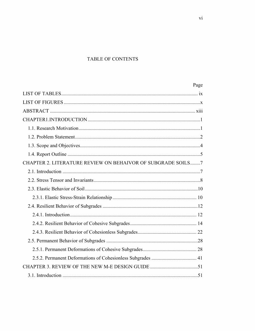
TABLE OF CONTENTS
Page
LIST OF TABLES............................................................................................................. ix
LIST OF FIGURES .............................................................................................................x
ABSTRACT .................................................................................................................... xiii
CHAPTER1.INTRODUCTION..........................................................................................1
1.1. Research Motivation.................................................................................................1
1.2. Problem Statement....................................................................................................2
1.3. Scope and Objectives................................................................................................4
1.4. Report Outline ..........................................................................................................5
CHAPTER 2. LITERATURE REVIEW ON BEHAIVOR OF SUBGRADE SOILS........7
2.1. Introduction ..............................................................................................................7
2.2. Stress Tensor and Invariants.....................................................................................8
2.3. Elastic Behavior of Soil ..........................................................................................10
2.3.1. Elastic Stress-Strain Relationship ................................................................... 10
2.4. Resilient Behavior of Subgrades ............................................................................12
2.4.1. Introduction..................................................................................................... 12
2.4.2. Resilient Behavior of Cohesive Subgrades..................................................... 14
2.4.3. Resilient Behavior of Cohesionless Subgrades............................................... 22
2.5. Permanent Behavior of Subgrades .........................................................................28
2.5.1. Permanent Deformations of Cohesive Subgrades........................................... 28
2.5.2. Permanent Deformations of Cohesionless Subgrades .................................... 41
CHAPTER 3. REVIEW OF THE NEW M-E DESIGN GUIDE ......................................51
3.1. Introduction ............................................................................................................51
vii
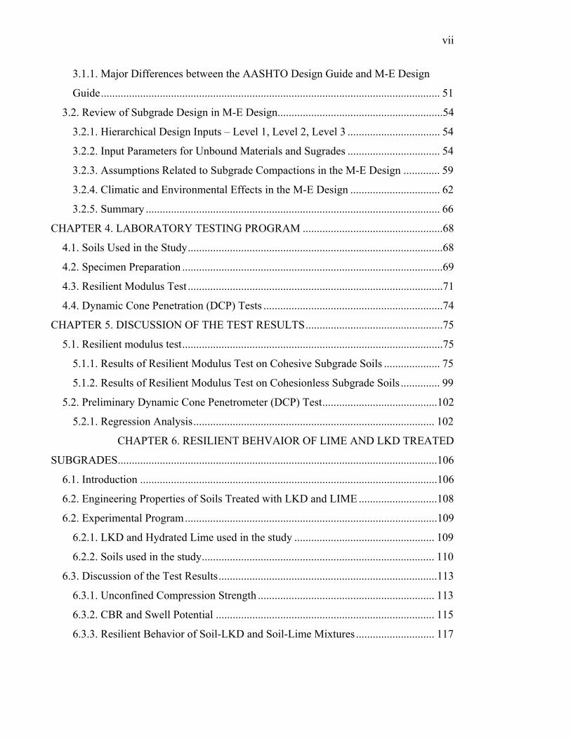
3.1.1. Major Differences between the AASHTO Design Guide and M-E Design
Guide......................................................................................................................... 51
3.2. Review of Subgrade Design in M-E Design...........................................................54
3.2.1. Hierarchical Design Inputs – Level 1, Level 2, Level 3 ................................. 54
3.2.2. Input Parameters for Unbound Materials and Sugrades ................................. 54
3.2.3. Assumptions Related to Subgrade Compactions in the M-E Design ............. 59
3.2.4. Climatic and Environmental Effects in the M-E Design ................................ 62
3.2.5. Summary ......................................................................................................... 66
CHAPTER 4. LABORATORY TESTING PROGRAM ..................................................68
4.1. Soils Used in the Study...........................................................................................68
4.2. Specimen Preparation .............................................................................................69
4.3. Resilient Modulus Test ...........................................................................................71
4.4. Dynamic Cone Penetration (DCP) Tests ................................................................74
CHAPTER 5. DISCUSSION OF THE TEST RESULTS.................................................75
5.1. Resilient modulus test.............................................................................................75
5.1.1. Results of Resilient Modulus Test on Cohesive Subgrade Soils .................... 75
5.1.2. Results of Resilient Modulus Test on Cohesionless Subgrade Soils .............. 99
5.2. Preliminary Dynamic Cone Penetrometer (DCP) Test.........................................102
5.2.1. Regression Analysis...................................................................................... 102
CHAPTER 6. RESILIENT BEHVAIOR OF LIME AND LKD TREATED
SUBGRADES..................................................................................................................106
6.1. Introduction ..........................................................................................................106
6.2. Engineering Properties of Soils Treated with LKD and LIME ............................108
6.2. Experimental Program..........................................................................................109
6.2.1. LKD and Hydrated Lime used in the study .................................................. 109
6.2.2. Soils used in the study................................................................................... 110
6.3. Discussion of the Test Results..............................................................................113
6.3.1. Unconfined Compression Strength ............................................................... 113
6.3.2. CBR and Swell Potential .............................................................................. 115
6.3.3. Resilient Behavior of Soil-LKD and Soil-Lime Mixtures ............................ 117
viii
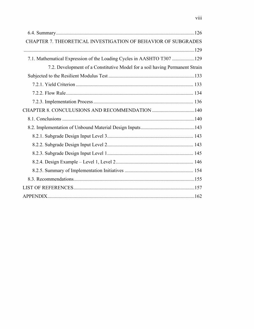
6.4. Summary...............................................................................................................126
CHAPTER 7. THEORETICAL INVESTIGATION OF BEHAVIOR OF SUBGRADES
.........................................................................................................................................129
7.1. Mathematical Expression of the Loading Cycles in AASHTO T307 ..................129
7.2. Development of a Constitutive Model for a soil having Permanent Strain
Subjected to the Resilient Modulus Test .....................................................................133
7.2.1. Yield Criterion .............................................................................................. 133
7.2.2. Flow Rule...................................................................................................... 134
7.2.3. Implementation Process ................................................................................ 136
CHAPTER 8. CONCULUSIONS AND RECOMMENDATION ..................................140
8.1. Conclusions ..........................................................................................................140
8.2. Implementation of Unbound Material Design Inputs...........................................143
8.2.1. Subgrade Design Input Level 3..................................................................... 143
8.2.2. Subgrade Design Input Level 2..................................................................... 143
8.2.3. Subgrade Design Input Level 1..................................................................... 145
8.2.4. Design Example – Level 1, Level 2.............................................................. 146
8.2.5. Summary of Implementation Initiatives ....................................................... 154
8.3. Recommendations.................................................................................................155
LIST OF REFERENCES.................................................................................................157
APPENDIX......................................................................................................................162
ix
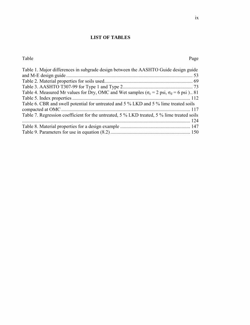
LIST OF TABLES
Table Page Table 1. Major differences in subgrade design between the AASHTO Guide design guide and M-E design guide ....................................................................................................... 53 Table 2. Material properties for soils used........................................................................ 69 Table 3. AASHTO T307-99 for Type 1 and Type 2......................................................... 73 Table 4. Measured Mr values for Dry, OMC and Wet samples (σc = 2 psi, σd = 6 psi ) .. 81 Table 5. Index properties ................................................................................................ 112 Table 6. CBR and swell potential for untreated and 5 % LKD and 5 % lime treated soils compacted at OMC ......................................................................................................... 117 Table 7. Regression coefficient for the untreated, 5 % LKD treated, 5 % lime treated soils......................................................................................................................................... 124 Table 8. Material properties for a design example ......................................................... 147 Table 9. Parameters for use in equation (8.2) ................................................................. 150
x
LIST OF FIGURES
Figure Page
Figure 1. Effect of deviator stress on a A-7-6 subgrade soil (Wilson et al. 1990) ........... 16 Figure 2. Effect of compaction water content and moisture density on a cohesive subgrade (Lee et al. 1997)................................................................................................. 18 Figure 3. Effect of post-compaction saturation on resilient modulus of an A-7-5 subgrade soil (Drumm et al. 1997)................................................................................................... 19 Figure 4. Effect of deviator stress on the resilient modulus of an A-1 subgrade soil (Wilson et al. 1990)........................................................................................................... 23 Figure 5. Influence of dry density on the resilient modulus of granular subgrades (Hicks and Monismith 1971)........................................................................................................ 24 Figure 6. Effect of method compaction (Lee et al. 1997)................................................. 25 Figure 7. Results from tests on compacted at dry of optimum A-6 subgrade soil (Muhanna et al. 1998) ....................................................................................................... 29 Figure 8. Results from tests on compacted at optimum A-6 subgrade soil (Muhanna et al. 1998) ................................................................................................................................. 29 Figure 9. Results from tests on compacted at wet of optimum A-6 subgrade soil (Muhanna et al. 1998) ....................................................................................................... 30 Figure 10. Results from tests on silty clay; left: σ3=0 psi, γd=129.5 lb/ft3, m=7% right: σ3=14.5 psi, γd=129.5 lb/ft3, m=7% (Raad and Zeid 1990).............................................. 31 Figure 11. Results from tests on silty clay; left: σ3=0 psi, γd=129.5 lb/ft3, m=10% right: σ3=14.5 psi, γd=129.5 lb/ft3, m=10% (Raad and Zeid 1990)............................................ 32 Figure 12. Influence of stress history on permanent strains (Monismith et al. 1975) ...... 33 Figure 13. Effect of period of rest on deformation under repeated loading of silty clay with high degree of saturation (Seed and Chan 1958)...................................................... 35 Figure 14. Effect of period of rest on deformation under repeated loading of silty clay with low degree of saturation (Seed and Chan, 1958) ...................................................... 36 Figure 15. Effect of frequency of stress application on deformation of silty clay with high degree of saturation (Seed and Chan 1958) ...................................................................... 37 Figure 16. Effect of frequency of stress application on deformation of silty clay with low degree of saturation (Seed and Chan 1958) ...................................................................... 38 Figure 17. Permanent axial strains for Sydenham sand (Gaskin et al. 1979) ................... 43 Figure 18. Plastic axial strains for Coteau Balast (Diyaljee and Raymond 1983)............ 44 Figure 19. Effect of confining stress on permanent strain at N=10,000 for the Florida subgrade sand (Pumphrey and Lentz 1986)...................................................................... 46 Figure 20. Effect of dry unit weight and moisture content on permanent strainat N=10,000 (Pumphrey and Lentz 1986) ............................................................................ 48

xi
Figure 21. Design inputs for unbound layers-response model ......................................... 55 Figure 22. Design inputs for unbound layers-ECIM inputs.............................................. 56 Figure 23. Variation in moisture contents for the compacted subgrade ........................... 61 Figure 24. Particle size distribution for soils used............................................................ 68 Figure 25. Compaction curves for soils used.................................................................... 71 Figure 26. Resilient modulus test equipment.................................................................... 72 Figure 27. Load pulse at a deviator stress of 2 psi............................................................ 73 Figure 28. Evaluation points of multi-elastic analyses for typical Indiana subgrades...... 76 Figure 29. Deviator stresses induced in the subgrade for cross-section 3 ........................ 77 Figure 30. Comparison of Mr between the Simplified (500 repetitions for conditioning and 100 repetitions for main testing) and the AASHTO procedures................................ 79 Figure 31. Comparison of Mr between the Simplified (250 repetitions for conditioning and 50 repetitions for main testing) and the AASHTO procedures between the Simplified........................................................................................................................................... 79 Figure 32. Unconfined compressive test results for Dry, OMC, Wet samples for I65-146........................................................................................................................................... 82 Figure 33. Unconfined compressive test results for Dry, OMC, Wet samples for I65-158........................................................................................................................................... 83 Figure 34. Unconfined compressive test results for Dry, OMC, Wet samples for I65-172........................................................................................................................................... 83 Figure 35. Unconfined compressive test results for Dry, OMC, Wet samples for Dsoil . 84 Figure 36. Permanent strains for I65-146 wet sample in the conditioning stage.............. 86 Figure 37. Permanent strains for I65-146 wet sample in the 5th step................................ 87 Figure 38. Mr values for original length and deformed length......................................... 87 Figure 39. Correlations between Mr and properties obtained from unconfined compressive tests .............................................................................................................. 91 Figure 40. Comparison between predicted and measured resilient moduli using equation (5.3)................................................................................................................................... 92 Figure 41.Comparison between predicted and measured resilient moduli using equation (5.4)................................................................................................................................... 95 Figure 42. Long-term resilient modulus testing for SR165 .............................................. 97 Figure 43. Long-term resilient modulus testing for Orchard clay .................................... 97 Figure 44. Permanent Strain of SR 165 Soil (long term Mr test) ..................................... 98 Figure 45. Permanent strain of SR 165 Soil (standard test).............................................. 99 Figure 46. Resilient modulus for US 50 ......................................................................... 100 Figure 47. Resilient modulus for Indiana dunes ............................................................. 100 Figure 48. Resilient modulus for N Dune....................................................................... 101 Figure 49. Resilient modulus for Wild Cat..................................................................... 101 Figure 50. Resilient modulus for SR 26.......................................................................... 102 Figure 51. Penetration Index vs. resilient modulus......................................................... 103 Figure 52. Penetration Index-1 vs. resilient modulus ...................................................... 104 Figure 53. Penetration Index-2 vs. resilient modulus ...................................................... 105 Figure 54. Particle size distribution for soils used.......................................................... 111 Figure 55. INDOT textural soil classification................................................................. 112 Figure 56. Compaction curves for soils used.................................................................. 113
xii
Figure 57. Unconfined strength vs. % compaction for A-4 (US-41).............................. 114 Figure 58. Unconfined strength vs. % compaction for A-6 (SR-37) ............................. 115 Figure 59. Resilient modulus vs. deviator stress for untreated soils for A-6 (SR-37).... 119 Figure 60. Resilient modulus vs. deviator stress for 5 % LKD treated soils for A-6 (SR-37)......................................................................................................................................... 120 Figure 61. Resilient modulus vs. deviator stress for 5 % Lime treated soils for A-6 (SR-37) ................................................................................................................................... 120 Figure 62. Resilient modulus vs. deviator stress for A-6 (SR-37) in terms of confining stress of 2 psi................................................................................................................... 121 Figure 63. Resilient modulus vs. deviator stress for A-7-6 (SR-46) in terms of confining stress of 2 psi................................................................................................................... 121 Figure 64. Resilient modulus vs. deviator stress for A-4 (US-41) in terms of confining stress of 2 psi................................................................................................................... 122 Figure 65. Resilient modulus vs. deviator stress for A-6 (US-41) in terms of confining stress of 2 psi................................................................................................................... 122 Figure 66. Measured vs. predicted Mr for untreated soils .............................................. 125 Figure 67. Measured vs. predicted Mr for 5 % LKD treated soils.................................. 125 Figure 68. Measured vs. predicted Mr for 5 % Lime treated soils ................................. 125 Figure 69. Loading cycle in AASTHO 307 test ............................................................. 131 Figure 70. Plot of F(t) as a function of time at a deviator stress of 2 psi........................ 132 Figure 71. Change in displacement with respect to time ................................................ 132 Figure 72. Comparison between the measured and predicted stress-strain relationship 139 Figure 73. Particle size distributions............................................................................... 147 Figure 74. Compaction curve following AASHTO T 99 ............................................... 148 Figure 75. Unconfined compressive tests for Dry, OMC and Wet samples................... 148 Figure 76. Resilient modulus test for OMC sample following AASHTO T-307........... 149 Figure 77. Resilient modulus test for wet sample following AASHTO T-307 .............. 149 Figure 78. Modulus ratio due to change in moisture ..................................................... 153 Figure 79. Comparison of permanent deformations (rutting) between optimum and average values................................................................................................................. 153 Figure 80. Modulus ratio due to change in moisture ...................................................... 154 Figure 81. Modulus ratio due to change in moisture (expanded) ................................... 154
1
CHAPTER1.INTRODUCTION
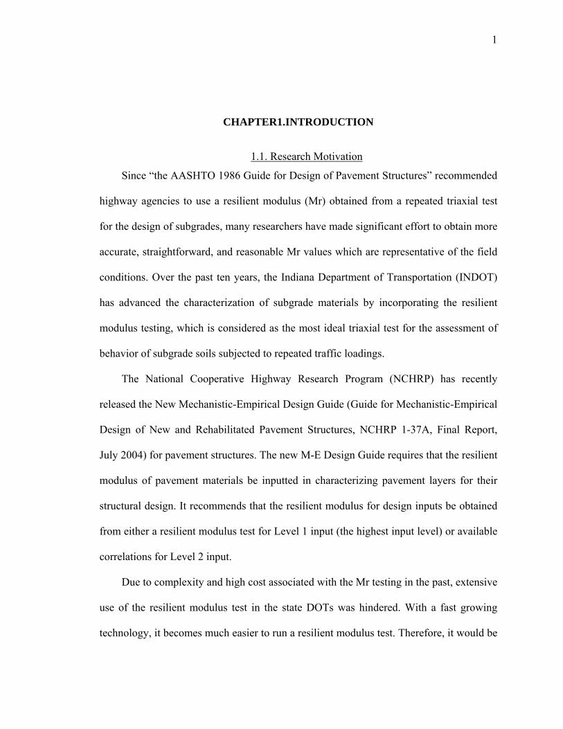
1.1. Research Motivation
Since “the AASHTO 1986 Guide for Design of Pavement Structures” recommended
highway agencies to use a resilient modulus (Mr) obtained from a repeated triaxial test
for the design of subgrades, many researchers have made significant effort to obtain more
accurate, straightforward, and reasonable Mr values which are representative of the field
conditions. Over the past ten years, the Indiana Department of Transportation (INDOT)
has advanced the characterization of subgrade materials by incorporating the resilient
modulus testing, which is considered as the most ideal triaxial test for the assessment of
behavior of subgrade soils subjected to repeated traffic loadings.
The National Cooperative Highway Research Program (NCHRP) has recently
released the New Mechanistic-Empirical Design Guide (Guide for Mechanistic-Empirical
Design of New and Rehabilitated Pavement Structures, NCHRP 1-37A, Final Report,
July 2004) for pavement structures. The new M-E Design Guide requires that the resilient
modulus of pavement materials be inputted in characterizing pavement layers for their
structural design. It recommends that the resilient modulus for design inputs be obtained
from either a resilient modulus test for Level 1 input (the highest input level) or available
correlations for Level 2 input.
Due to complexity and high cost associated with the Mr testing in the past, extensive
use of the resilient modulus test in the state DOTs was hindered. With a fast growing
technology, it becomes much easier to run a resilient modulus test. Therefore, it would be
2
necessary for the department of transportation to appropriately implement the resilient
modulus test for an improved design of subgrades.
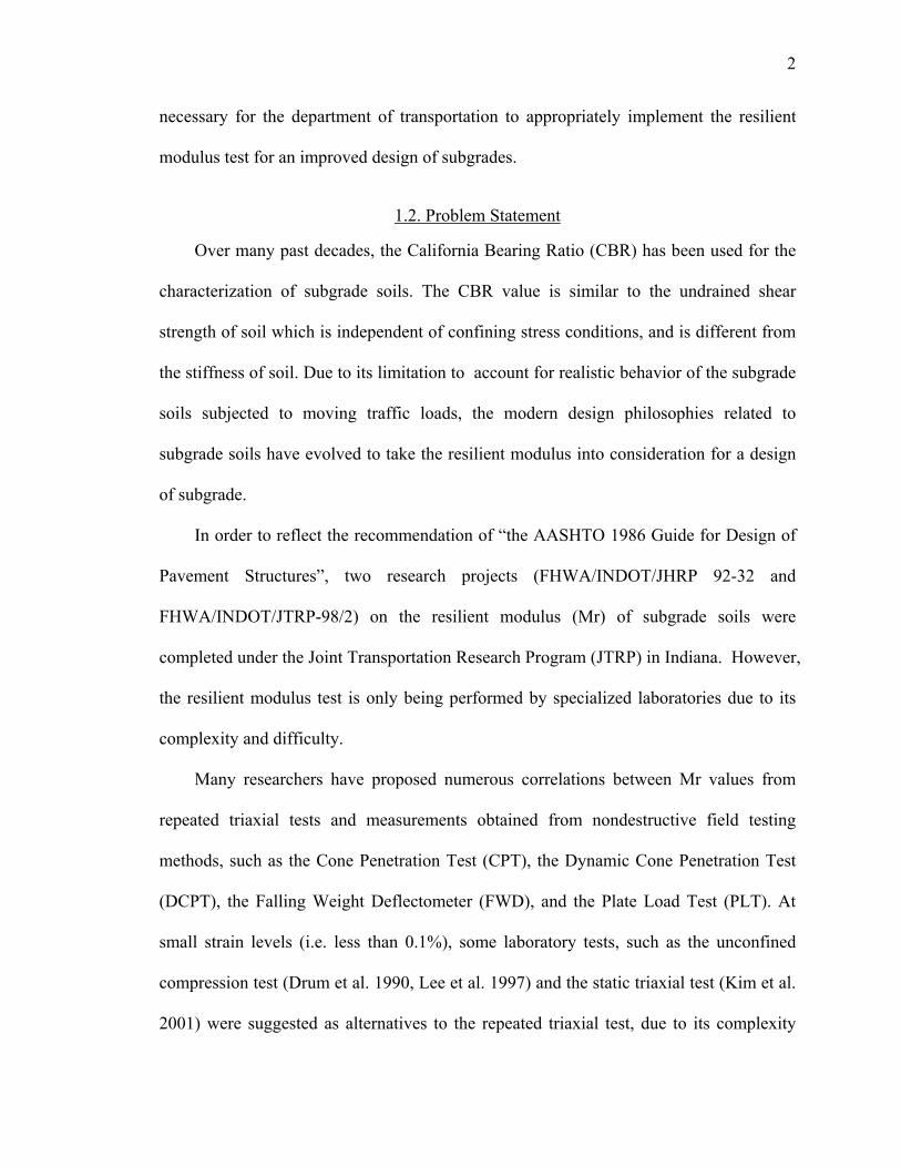
1.2. Problem Statement
Over many past decades, the California Bearing Ratio (CBR) has been used for the
characterization of subgrade soils. The CBR value is similar to the undrained shear
strength of soil which is independent of confining stress conditions, and is different from
the stiffness of soil. Due to its limitation to account for realistic behavior of the subgrade
soils subjected to moving traffic loads, the modern design philosophies related to
subgrade soils have evolved to take the resilient modulus into consideration for a design
of subgrade.
In order to reflect the recommendation of “the AASHTO 1986 Guide for Design of
Pavement Structures”, two research projects (FHWA/INDOT/JHRP 92-32 and
FHWA/INDOT/JTRP-98/2) on the resilient modulus (Mr) of subgrade soils were
completed under the Joint Transportation Research Program (JTRP) in Indiana. However,
the resilient modulus test is only being performed by specialized laboratories due to its
complexity and difficulty.
Many researchers have proposed numerous correlations between Mr values from
repeated triaxial tests and measurements obtained from nondestructive field testing
methods, such as the Cone Penetration Test (CPT), the Dynamic Cone Penetration Test
(DCPT), the Falling Weight Deflectometer (FWD), and the Plate Load Test (PLT). At
small strain levels (i.e. less than 0.1%), some laboratory tests, such as the unconfined
compression test (Drum et al. 1990, Lee et al. 1997) and the static triaxial test (Kim et al.
2001) were suggested as alternatives to the repeated triaxial test, due to its complexity
3
and difficulty. Therefore, there is a need to simplify the complex procedure of the
existing resilient modulus test to allow the operator of the resilient modulus testing to
readily perform the Mr test.
Note that the AASHTO Design guide recommends highway agencies to use
representative confining and deviator stresses in subgrade layers under traffic loading
conditions. When simplifying the Mr test procedure, it is necessary to investigate the
range of confining and deviator stresses resulting from the traffic loadings in Indiana and
to account for such reasonable stress levels in the Mr test. Over- or underestimation of the
stress levels in the subgrades will lead to erroneous results of resilient modulus results
(Houston et al. 1993). As one resilient modulus corresponding to the representative
confining and deviator stress for a given subgrade is needed in designing a pavement, the
complex testing procedure may be simplified for practical design purpose.
In the previous JTRP project, resilient modulus tests based on AASHTO T 274 were
performed by Lee et al. (1993) on several predominant soils and correlations were made
between the resilient modulus and the unconfined compressive strength. However, using
their correlations for all of subgrade soils encountered in Indiana is not feasible as their
correlations are not based on the soil properties. Moreover, the resilient modulus test
method has been changed to AASHTO T307. In order to successfully design subgrades
following the New M-E Design Guide, predictive models based on the soil properties,
standard Proctor tests, and unconfined compressive tests are necessary for designers to
use those models conveniently for wide range of subgrade soils encountered in Indiana.
The basic principle of the loading adopted in AASHTO T 307 is the simulation of a
typical moving load in a sinusoidal form. The peak point of the loading is analogous to

4
the loading condition where the traffic is immediately above the subgrade. A soil
specimen subjected to resilient modulus testing can be simply modeled as a one-
dimensional forced vibration of a spring-mass system and the feasibility of the
mathematical approach needs to be explored to suggest a simple calculation method to
obtain the resilient modulus.
Generally, the permanent strain of subgrade soils is not taken into consideration in
the resilient modulus test. This is due to the assumption that the subgrade would be in the
elastic state. However, subgrade soils may exhibit the permanent strain even at a much
smaller load than that causing shear failure. It is fairly necessary to develop a constitutive
model that describes the realistic behavior of subgrade soils, such as resilient and
permanent behavior.
1.3. Scope and Objectives
The objectives of this study are to simplify the resilient modulus testing procedure
specified in AASHTO T307 based on the prevalent conditions in Indiana, to generate
database of Mr values following the existing resilient modulus test method (AASHTO
T307) for Indiana subgrades, to develop useful predictive models for use in Level 1 and
Level 2 input of subgrade Mr values following the New M-E Design Guide, to develop a
simple calculation method, and to develop a constitutive model based on the Finite
Element Method (FEM) to account for both the resilient and permanent behavior of
subgrade soils. The detailed goals of the research will be:
(1) Simplification of the standard resilient modulus testing;
5
(2) Clarification of confining pressure effects on resilient modulus of cohesive
subgrades;
(3) Construction of database of resilient modulus depending on soil types in Indiana;
(4) Development of predictive models to estimate the resilient moduli for subgrades
encountered in Indiana;
(5) Development of a simple mathematical method to calculate the resilient modulus;
(6) Development of a constitutive model based on the Finite Element Method that can
describe both resilient and permanent behavior of subgrade soils.
1.4. Report Outline
This report consists of eight chapters, including this introduction.
Chapter 2 presents the literature review on the resilient behavior and permanent
behavior of cohesive and cohesionless soils, and fundamental theories related to behavior
of subgrade soils.
Chapter 3 reviews the important features embedded in “the New Mechanistic-
Empirical Design Guide”.
Chapter 4 describes the experimental program of the project. This chapter covers
the soils used, resilient modulus tests, unconfined compressive tests, physical property
tests and DCPT tests.
Chapter 5 discusses the results of resilient modulus tests on compacted subgrade
soils. Predictive models to estimate resilient modulus based on soil properties are
discussed.
Chapter 6 reports the results of resilient modulus tests on chemically modified soils
which were previously conducted as part of implementation.
6
Chapter 7 introduces a simple mathematical method to obtain resilient modulus and
a constitutive model based on Finite Element Method that can describe permanent and
resilient behavior.
Chapter 8 summarizes the conclusions and recommendations drawn from this study
and proposes implementation initiatives.

7
CHAPTER 2. LITERATURE REVIEW ON BEHAIVOR OF SUBGRADE SOILS
2.1. Introduction
In a road structure subjected to repeated traffic loadings, subgrade soils play a role
in supporting the asphalt and base layers and traffic loadings. Due to this important role,
the subgrade should have enough bearing capacity to perform its function appropriately.
If the subgrade soils respond primarily in an elastic mode, the rutting problem typical in
weak subgrades will not occur.
However, rutting problems are observed in many roads, resulting in expensive
rehabilitation efforts. Therefore, the assumption that subgrade soils are purely elastic is
not consistent with most observation mode in practice. It is more realistic to treat the
subgrade soils as elasto-plastic materials. In reality, subgrade soils subjected to repeated
traffic loadings exhibit nonlinear resilient and permanent behavior even at small strains,
before reaching their yield strengths.
In this chapter, to facilitate the understanding of the resilient and permanent
behavior of subgrade soils, the following topics will be discussed: stress tensors and
invariants, elastic stress-strain relationship, resilient and permanent behavior of subgrade.
8
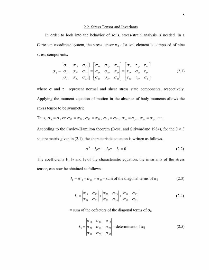
2.2. Stress Tensor and Invariants
In order to look into the behavior of soils, stress-strain analysis is needed. In a
Cartesian coordinate system, the stress tensor σij of a soil element is composed of nine
stress components:
⎥⎥⎥
⎦
⎤
⎢⎢⎢
⎣
⎡=
333231
232221
131211
σσσσσσσσσ
σ ij ≡⎥⎥⎥
⎦
⎤
⎢⎢⎢
⎣
⎡
zzzyzx
yzyyyx
xzxyxx
σσσσσσσσσ
≡⎥⎥⎥
⎦
⎤
⎢⎢⎢
⎣
⎡
zzyzx
yzyyx
xzxyx
στττστττσ
(2.1)
where σ and τ represent normal and shear stress state components, respectively.
Applying the moment equation of motion in the absence of body moments allows the
stress tensor to be symmetric.
Thus, jiij σσ = or 2112 σσ = , 3113 σσ = , 3223 σσ = , yxxy σσ = , zyyz σσ = , etc.
According to the Cayley-Hamilton theorem (Desai and Siriwardane 1984), for the 3 × 3
square matrix given in (2.1), the characteristic equation is written as follows.
0322
13 =−+− III σσσ (2.2)
The coefficients I1, I2 and I3 of the characteristic equation, the invariants of the stress
tensor, can now be obtained as follows.
3322111 σσσ ++=I = sum of the diagonal terms of σij (2.3)
3313
1311
3323
2322
2221
12112 σσ
σσσσσσ
σσσσ
++=I (2.4)
= sum of the cofactors of the diagonal terms of σij
333231
232221
131211
3
σσσσσσσσσ
=I = determinant of σij (2.5)

9
I1, I 2 and I3 are called invariants because they do not change when the coordinate axes are
rotated. Although there is a change of coordinates, the principal stresses and principal
axes remain the same. The first invariant I1 is often referred to as bulk stress θ.
In order to express the stress state for a soil in 3D space, principal stresses are
generally used because the principal stresses are also invariants regardless of rotation of
axes. Now expressing the stress tensor in terms of principal stresses, (2.1) becomes
⎥⎥⎥
⎦
⎤
⎢⎢⎢
⎣
⎡=
3
2
1
000000
σσ
σσ ij (2.6)
when σ1 > σ2 > σ3, σ1, σ2, and σ3 are major, intermediate and minor pricipal stresses,
respectively.
A more accessible formulation results by decomposing a stress tensor into a
deviatoric tensor and a hydrostatic tensor, because the characteristics of shear and mean
stresses for a soil become more evident. Equation 2.7 illustrates this relationship.
ijnnijij S δσσ31
+= (2.7)
where Sij = deviatoric tensor, σnn = hydrostatic stress = σ11+ σ22 + σ33, δij = Kronecker
delta.
Substitution of (2.7) into equation (2.1) leads to:
⎥⎥⎥
⎦
⎤
⎢⎢⎢
⎣
⎡
333231
232221
131211
σσσσσσσσσ
= ⎥⎥⎥
⎦
⎤
⎢⎢⎢
⎣
⎡
333231
232221
131211
SSSSSSSSS
+
⎥⎥⎥⎥⎥⎥
⎦
⎤
⎢⎢⎢⎢⎢⎢
⎣
⎡
300
03
0
003
nn
nn
nn
σ
σ
σ
(2.8)
Thus,
10
ijnnijijS δσσ31
−= = ijij pδσ − (2.9)
where p = mean stress = σnn/3
Because the deviatoric stress tensor is also a symmetric tensor, the deviatoric stress
invariants are obtained as follows.
03322111 =++== SSSSJ ii (2.10)
[ ]233
223
213
223
222
212
213
212
2112 2
121 SSSSSSSSSSSJ ijij ++++++++== (2.11)
( )[ ]231
232
221 )()(
61 σσσσσσ −+−+−= (2.12)
0272
32
31 3
12133 =+−== IIIISSSJ mijmij (2.13)
2.3. Elastic Behavior of Soil
2.3.1. Elastic Stress-Strain Relationship
This first step in describing elasto-plastic behavior is to define elastic behavior. A
solid is called elastic if it completely recovers its original configuration when the forces
applied on it are removed. According to the generalized form of Hooke’s law, the linear
elastic relationship between the stress tensor and strain tensor can be written as follows
(Chen and Saleeb 1994).
klijklij C εσ = (2.14)
11
Here Cijkl is a fourth-order elastic stiffness tensor and has 81 constants. By using the
symmetry of stress, strain and elastic stiffness tensors, 81 constants reduce to 21
constants (Chen and Saleeb 1994). Now (2.14) can be expressed in matrix form as:
⎪⎪⎪
⎭
⎪⎪⎪
⎬
⎫
⎪⎪⎪
⎩
⎪⎪⎪
⎨
⎧
⎥⎥⎥⎥⎥⎥⎥
⎦
⎤
⎢⎢⎢⎢⎢⎢⎢
⎣
⎡
=
⎪⎪⎪
⎭
⎪⎪⎪
⎬
⎫
⎪⎪⎪
⎩
⎪⎪⎪
⎨
⎧
13
23
12
33
22
11
121212131223123312221211
131213131323133313221311
231223132323233323222311
331233133323333333223311
221222132223223322222211
111211131123113311221111
12
13
23
33
22
11
γγγεεε
σσσσσσ
CCCCCCCCCCCCCCCCCCCCCCCCCCCCCCCCCCCC
where ε11, ε22, and ε33 are normal strains, and γ12, γ23, and γ13 are shear strains,
respectively.
In the most general form, an isotropic, fourth-order tensor can be given by:
jkiljlikklijijklC δνδδμδδλδ ++= (2.15)
Since Cijkl is symmetric and hence μ = ν, taking (2.15) into (2.14) leads to:
ijkkijij μεελδσ 2+= (2.16)
where λ and μ are Lame’s constants. Here μ is the shear modulus, also known as G.
In order to express ε in terms of σ, rewriting (2.16) leads to:
kkij
ijij σμλμ
λδσ
με
)23(221
+−= (2.17)
Matrix C-1 becomes

12
⎥⎥⎥⎥⎥⎥⎥⎥⎥⎥
⎦
⎤
⎢⎢⎢⎢⎢⎢⎢⎢⎢⎢
⎣
⎡
++
+
+−−
−+−
−−+
+=−
μλμλ
μλ
μλλλ
λμλλ
λλμλ
μμ
230000002300000023000
00022
00022
00022
)23(11C
Young’s modulus E, Poisson’s ratio ν, shear modulus G, and bulk modulus K can be
defined as:
)()23(
μλμλμ
++
=E (2.18)
)(2 μλλν+
= (2.19)
)1(2 νμ
+==
EG (2.20)
)21(33 νεσ
−==
EKkk
kk (2.21)
These fundamental elastic terms discussed above will be used in developing a
constitutive model that describes both resilient and permanent behavior in the finite
element (FE) formulation in Chapter 7.
2.4. Resilient Behavior of Subgrades
2.4.1. Introduction
It is well known that subgrade soils show a nonlinear and time dependent elasto-
plastic response under traffic loading. As mentioned earlier, in the traditional theories of
13
elasticity, the elastic properties of a material are defined by the elastic modulus E and
Poisson’s ratio ν. A similar approach has been widely used in dealing with base material
and subgrade soils. In this approach, the elastic modulus is replaced with the resilient
modulus to represent the nonlinearity with respect to stress level (Lekarp et al. 2000).
This resilient modulus is generally used as an input parameter for multi-layered elastic
analysis. The resilient modulus is very meaningful to a pavement’s life. To illustrate this
condition, Elliott and Thornton (1988) reported the results of analyses using the ILLI-
PAVE algorithms on a flexible pavement subjected to a 9,000-pound wheel load. As the
resilient modulus increased, the asphalt layer strain decreased and the subgrade stress
ratio (load-induced deviator stress in subgrade divided by the unconfined compressive
strength of the soil) also decreased.
From 1986, AASHTO required the use of the subgrade resilient modulus for the
design of flexible pavements. Resilient modulus is an important material property, similar
in concept to the modulus of elasticity. It differs from the modulus of elasticity in that it
is obtained by a repeated-load triaxial test and is based only on the recoverable strains.
Resilient modulus is defined as:
r
dRM
εσ
= (2.22)
where MR is the resilient modulus; σd is the repeated deviator stress; and εr is the
recoverable axial strain.
The current standard test method to determine the resilient modulus is described by
AASHTO T 307-99 which has recently been upgraded from AASHTO T 294-94 and
AASHTO T 274. Most literature is limited to AASHTO T 294-94 and AASHTO T 274
14
but limited literature on the evaluation of AASHTO T 307-99 appears to be available. In
AASHTO T 307-99, traffic conditions are simulated by applying a series of repeated
deviator stresses, separated by rest periods and field conditions are simulated by
conditioning and postconditioning (i.e. main testing). Conditioning consists of 500 to
1000 load applications at a confining stress of 6 psi and a deviator stress of 4 psi. In
addition, main testing is performed at three levels of confining stresses (2, 4, 6 psi) for
which each 5 levels of deviator stresses (2, 4, 6, 8 and 10 psi) are applied, resulting in 15
steps of load applications. AASHTO T 307-99 classifies soil types into type 1 and type 2
materials. Granular soils and cohesive soils are categorized as type 1 and type 2,
respectively. This test applies to the same procedure for both granular and cohesive
subgrades and is done under drained conditions only. However, the research on the
drainage condition has been quite limited and somewhat neglected. Although the test is
done under drained conditions, considerably fast and repeated load applications (each
cycle consists of 0.1 second loading and 0.9 second unloading) may lead to undrained or
partially undrained condition, especially for cohesive subgrades.
2.4.2. Resilient Behavior of Cohesive Subgrades
In general, the resilient modulus of cohesive subgrades is affected by the following
factors: a) Deviator stress; b) Method of compaction; c) Compaction water content and
dry density; d) Thixotropy; e) Degree of saturation; and f) Freeze-thaw cycles. Deviator
stress, compaction water content and dry density, and freeze-thaw cycles are the factors
that most influence the resilient modulus of cohesive subgrades. Another factor that
affects the resilient modulus is seasonal variation of moisture content. Seasonal variations,
15
however, can be accounted for by variations in the degree of saturation. Therefore,
seasonal variations will not be discussed further here.
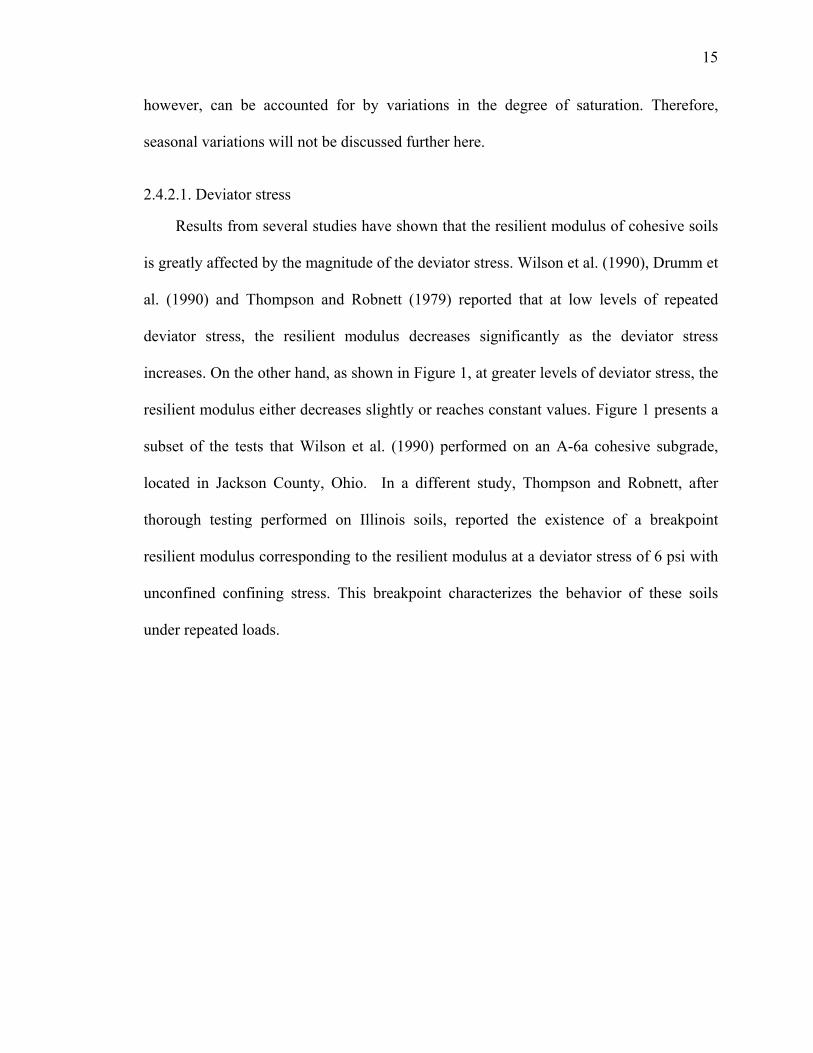
2.4.2.1. Deviator stress
Results from several studies have shown that the resilient modulus of cohesive soils
is greatly affected by the magnitude of the deviator stress. Wilson et al. (1990), Drumm et
al. (1990) and Thompson and Robnett (1979) reported that at low levels of repeated
deviator stress, the resilient modulus decreases significantly as the deviator stress
increases. On the other hand, as shown in Figure 1, at greater levels of deviator stress, the
resilient modulus either decreases slightly or reaches constant values. Figure 1 presents a
subset of the tests that Wilson et al. (1990) performed on an A-6a cohesive subgrade,
located in Jackson County, Ohio. In a different study, Thompson and Robnett, after
thorough testing performed on Illinois soils, reported the existence of a breakpoint
resilient modulus corresponding to the resilient modulus at a deviator stress of 6 psi with
unconfined confining stress. This breakpoint characterizes the behavior of these soils
under repeated loads.
16
Figure 1. Effect of deviator stress on a A-7-6 subgrade soil (Wilson et al. 1990)
2.4.2.2. Method of compaction
Lee (1993) reported on the influence of the method of compaction on the resilient
modulus of cohesive subgrades based on the results of past studies. For specimens
compacted at low degrees of saturation, the method of compaction had little effect on the
resilient modulus due to the flocculated arrangement of the clay particles. In contrast,
when samples are compacted above optimum water content, compaction caused large
changes, which was attributed to the dispersed arrangement of the clay particles. Seed
and Chan (1959) concluded that the kneading and impact methods of compaction usually
produce a flocculated particle arrangement for water contents dry of optimum and a
dispersed arrangement at wet of optimum, while static compaction, at any level of
moisture content generates a flocculated arrangement. They also reported that for clays
Deviator Stress (psi)
MR (ksi)
17
compacted dry of optimum, the recoverable strains for samples prepared by kneading and
static compaction were the same. However, for specimens compacted wet of optimum,
the kneading compacted specimens experienced significantly larger recoverable strains.
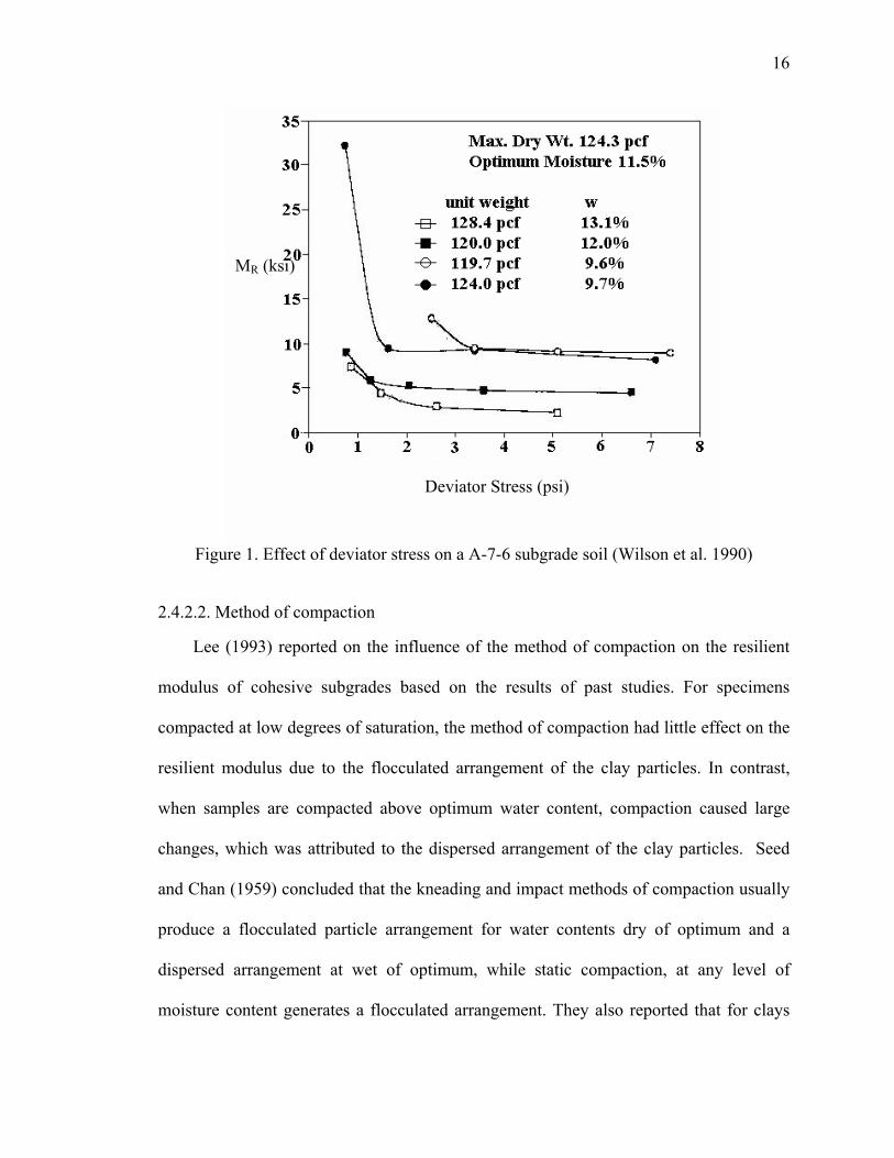
2.4.2.3. Compaction water content and dry density
It is expected that as the compaction moisture content of a cohesive soil increases,
the stiffness of the soil tends to decrease. As seen from Figures 2 and 3, the same trend
has been observed for the resilient modulus. Figure 2 is from results of tests on cohesive
subgrades conducted in Indiana by Lee et al. (1997). Figures 1 and 2 clearly show that as
the moisture content increases, the resilient modulus decreases. It was noticed that
specimens compacted wet of optimum exhibit significantly lower values of the resilient
modulus. This observation agrees well with the aforementioned effect of the method of
compaction. As seen from Figure 2, it is also observed that the resilient modulus
increases as the dry density increases. As the density of any soil increases, less volume is
occupied by the voids, and this consequently results in the increase of the strength of the
soil.

18
Figure 2. Effect of compaction water content and moisture density on a cohesive subgrade (Lee et al. 1997)
2.4.2.4. Thixotropy
Seed and Chan (1957) showed that when samples of cohesive soil are compacted at
a high degree of saturation, they exhibit a significant increase in strength if they are
allowed to rest before testing. Seed and Chan also reported that after a certain number of
repeated loads (about 40,000 repetitions), thixotropy no longer affected the recoverable
deformations. This situation could be attributed to the fact that the induced deformations
were so large that they overcame the thixotropic strength of the samples.
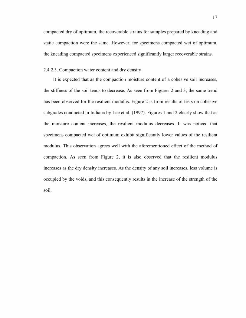
2.4.2.5. Degree of saturation
The effect of the degree of saturation is similar to the effect of the water content on
the resilient modulus. Figure 3 presents the variation of the resilient modulus with the
degree of saturation of an A-7-5 subgrade soil, compacted wet of optimum. The results
Moisture content (%)
Dry unit weight kN/m³
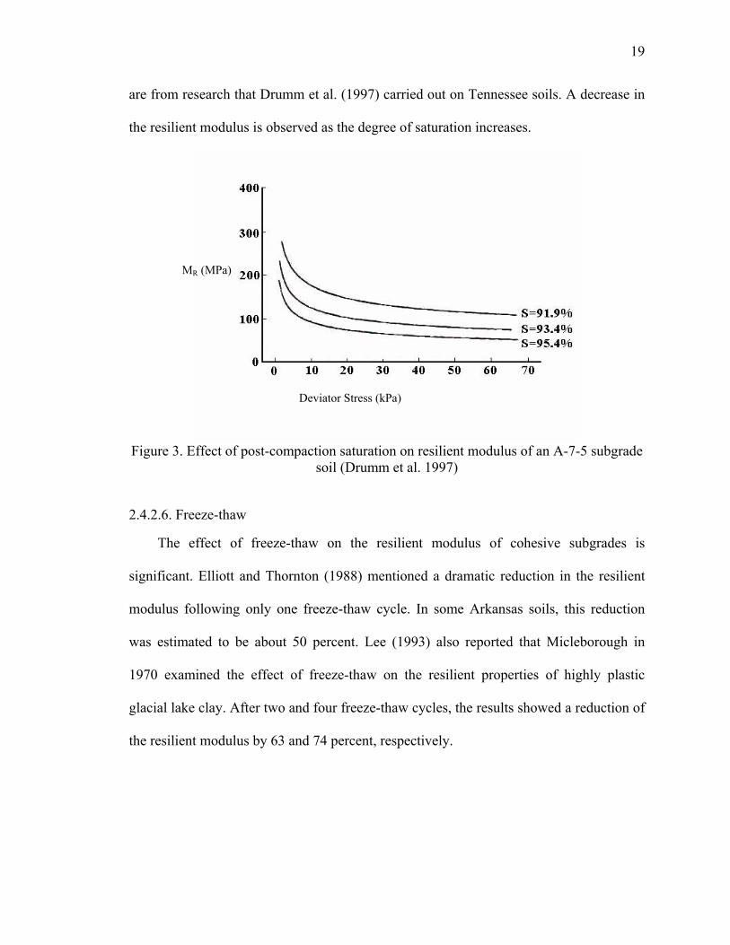
19
are from research that Drumm et al. (1997) carried out on Tennessee soils. A decrease in
the resilient modulus is observed as the degree of saturation increases.
Figure 3. Effect of post-compaction saturation on resilient modulus of an A-7-5 subgrade
soil (Drumm et al. 1997)
2.4.2.6. Freeze-thaw
The effect of freeze-thaw on the resilient modulus of cohesive subgrades is
significant. Elliott and Thornton (1988) mentioned a dramatic reduction in the resilient
modulus following only one freeze-thaw cycle. In some Arkansas soils, this reduction
was estimated to be about 50 percent. Lee (1993) also reported that Micleborough in
1970 examined the effect of freeze-thaw on the resilient properties of highly plastic
glacial lake clay. After two and four freeze-thaw cycles, the results showed a reduction of
the resilient modulus by 63 and 74 percent, respectively.
Deviator Stress (kPa)
MR (MPa)
20
2.4.2.7. Models for the resilient modulus of cohesive subgrades
During the last twenty years, many models have been proposed to predict the
resilient modulus of cohesive subgrades. Some of them are stress-dependent and others
are dependent on physical properties. There are also models that considered both physical
and stress conditions of the subgrades. However, all these models seem to apply only to
the subgrades that were used to develop these models. In most of the cases when the
models were applied to other types of cohesive subgrades, the deviation was significant.
This deviation is expected given the nature of the models. These models were developed
for certain soils and then were examined to see if they were applicable to others. The
results were not satisfactory because these soils had different physical and stress
conditions. Therefore, it is worth noting that when using one of the models presented next,
one must proceed with caution.
a. Pezo and Hudson (1994) suggested the following model for the resilient modulus.
6543210 FFFFFFFMr ⋅⋅⋅⋅⋅⋅= , 803.02 =R (2.23)
Factors F0 ~ F6 depend on physical properties and the stress condition of the soil.
b. Thompson and Robnett (1979) introduced the following model.
)( 132 dkkkMr σ−⋅+= , if k1>σd (2.24)
)( 142 kkkMr d −⋅+= σ , if k1<σd (2.25)
k1 - k4 = material and physical property parameters.
c. Hall and Thompson (1994) proposed the model:
CPICOPTMr ⋅−⋅+⋅+= 970.1216.00064.090.6)( , 76.02 =R (2.26)

21
Mr (OPT): subgrade resilient modulus (ksi) at AASHTO T-99 optimum moisture
content and 95 percent compaction
C: percent clay (<2μm)
PI: plasticity index (percent)
OC: percent organic carbon
R2: coefficient of determination
d. Lee et al. (1979) suggested the following model.
2%0.1%0.1 )(93.5)(4.695 uu SSMr ⋅−⋅= , 97.02 =R (2.27)
Mr: resilient modulus (psi) at maximum axial stress of 6psi, confining stress is 3psi
Su1.0%: stress (psi) causing 1% strain in conventional unconfined compressive test
e. Mohammad et al. (1999) performed CPT tests in two types of clay and suggested the
model below.
edwcfbqaMr dsnc +⋅+⋅+⋅+⋅= γ , 95.091.02 −=R (2.28)
Mr: resilient modulus (in MPa)
a, b, c, d, e: constants from regression analyses
n: integer (1, 2, or 3)
qc: tip resistance (MPa)
fs: sleeve friction (MPa)
w:moisture content (%)
γd : dry unit weight (kN/m3)
f. Drumm et al. (1997) modeled the change of the resilient modulus with respect to post-
compaction saturation and presented the following model.
22
SdS
dMMM roptrwetr Δ⋅+= )()( (2.29)
Mr(wet): resilient modulus (MPa) at increased post-compaction saturation
M r(opt): resilient modulus (MPa) at optimum moisture content
dMr/dS: gradient of resilient modulus (MPa), function of type of soil
ΔS: change in post-compaction degree of saturation (decimal)
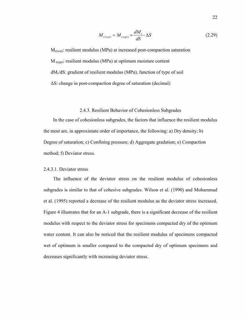
2.4.3. Resilient Behavior of Cohesionless Subgrades
In the case of cohesionless subgrades, the factors that influence the resilient modulus
the most are, in approximate order of importance, the following: a) Dry density; b)
Degree of saturation; c) Confining pressure; d) Aggregate gradation; e) Compaction
method; f) Deviator stress.
2.4.3.1. Deviator stress
The influence of the deviator stress on the resilient modulus of cohesionless
subgrades is similar to that of cohesive subgrades. Wilson et al. (1990) and Mohammad
et al. (1995) reported a decrease of the resilient modulus as the deviator stress increased.
Figure 4 illustrates that for an A-1 subgrade, there is a significant decrease of the resilient
modulus with respect to the deviator stress for specimens compacted dry of the optimum
water content. It can also be noticed that the resilient modulus of specimens compacted
wet of optimum is smaller compared to the compacted dry of optimum specimens and
decreases significantly with increasing deviator stress.

23
Figure 4. Effect of deviator stress on the resilient modulus of an A-1 subgrade soil (Wilson et al. 1990)
2.4.3.2. Confining pressure
The effect of confining pressure on granular subgrades is more pronounced than the
effect of the deviator stress. Mohammad et al. (1995) and Hicks and Monismith (1971)
reported that the resilient modulus of granular subgrades increases as the confining
pressure increases.
2.4.3.3. Dry density
Dry density has a significant role in the resilient modulus of cohesionless subgrades.
Lee et al. (1995) reported that specimens of dune sand exhibited higher values of resilient
modulus as the dry density increased. Moreover, Hicks and Monismith (1971) concluded
from tests performed on a granular subgrade (shown in Figure 5) that the resilient
Mr (ksi)
Deviator Stress (psi)
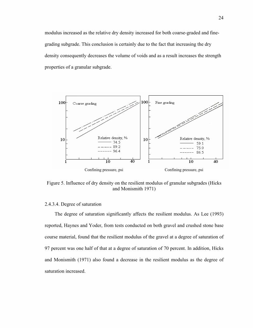
24
modulus increased as the relative dry density increased for both coarse-graded and fine-
grading subgrade. This conclusion is certainly due to the fact that increasing the dry
density consequently decreases the volume of voids and as a result increases the strength
properties of a granular subgrade.
Figure 5. Influence of dry density on the resilient modulus of granular subgrades (Hicks and Monismith 1971)
2.4.3.4. Degree of saturation
The degree of saturation significantly affects the resilient modulus. As Lee (1993)
reported, Haynes and Yoder, from tests conducted on both gravel and crushed stone base
course material, found that the resilient modulus of the gravel at a degree of saturation of
97 percent was one half of that at a degree of saturation of 70 percent. In addition, Hicks
and Monismith (1971) also found a decrease in the resilient modulus as the degree of
saturation increased.
Confining pressure, psi Confining pressure, psi
25
2.4.3.5. Aggregate gradation
Hicks and Monismith (1971) examined the effect of aggregate gradation. As
presented in Figure 5, as the percentage of fines increased in a granular subgrade, for the
same level of confining pressure, a decrease of the resilient modulus was observed. As
the percentage of fines increases in a granular soil, the degree of interlocking decreases
which results in the decrease of the strength of the soil.
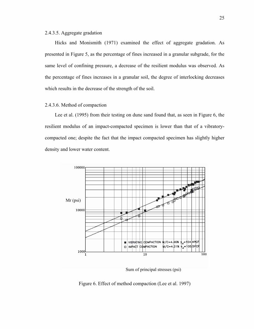
2.4.3.6. Method of compaction
Lee et al. (1995) from their testing on dune sand found that, as seen in Figure 6, the
resilient modulus of an impact-compacted specimen is lower than that of a vibratory-
compacted one; despite the fact that the impact compacted specimen has slightly higher
density and lower water content.
Figure 6. Effect of method compaction (Lee et al. 1997)
Sum of principal stresses (psi)
Mr (psi)

26
2.4.3.7. Models for the resilient modulus of cohesionless subgrades
The models proposed to predict the resilient modulus of granular subgrades do not
fit well to soils other than those for which the models were developed. One example is
the case of Puppala et al. (1996) who used three models to predict the resilient modulus
of sand. Among those three models, the triaxial model provided predictions closer to the
measured data. The other two models deviated significantly from the measured data. The
following are some examples of models used to predict the resilient modulus of granular
subgrade.
a. Lee et al. (1995) from their tests on dune sand proposed the following model.
595.0)886.232163,20( θ⋅⋅+−= RCMr (2.30)
MR: resilient modulus (kPa)
RC: relative compaction = dry density/17.17kN/m3
θ: sum of principal stresses (kPa)
b. Puppala et al. (1996), in their study to predict the resilient modulus of a sand, used the
following three equations.
(Bulk stress model)
baMr θ⋅= (2.31a)
wa d ⋅−⋅+−= 27.006.085.0log γ , 98.02 =R (2.31b)
wb d ⋅+⋅+−= 11.0002.023.1 γ , 96.02 =R (2.31c)
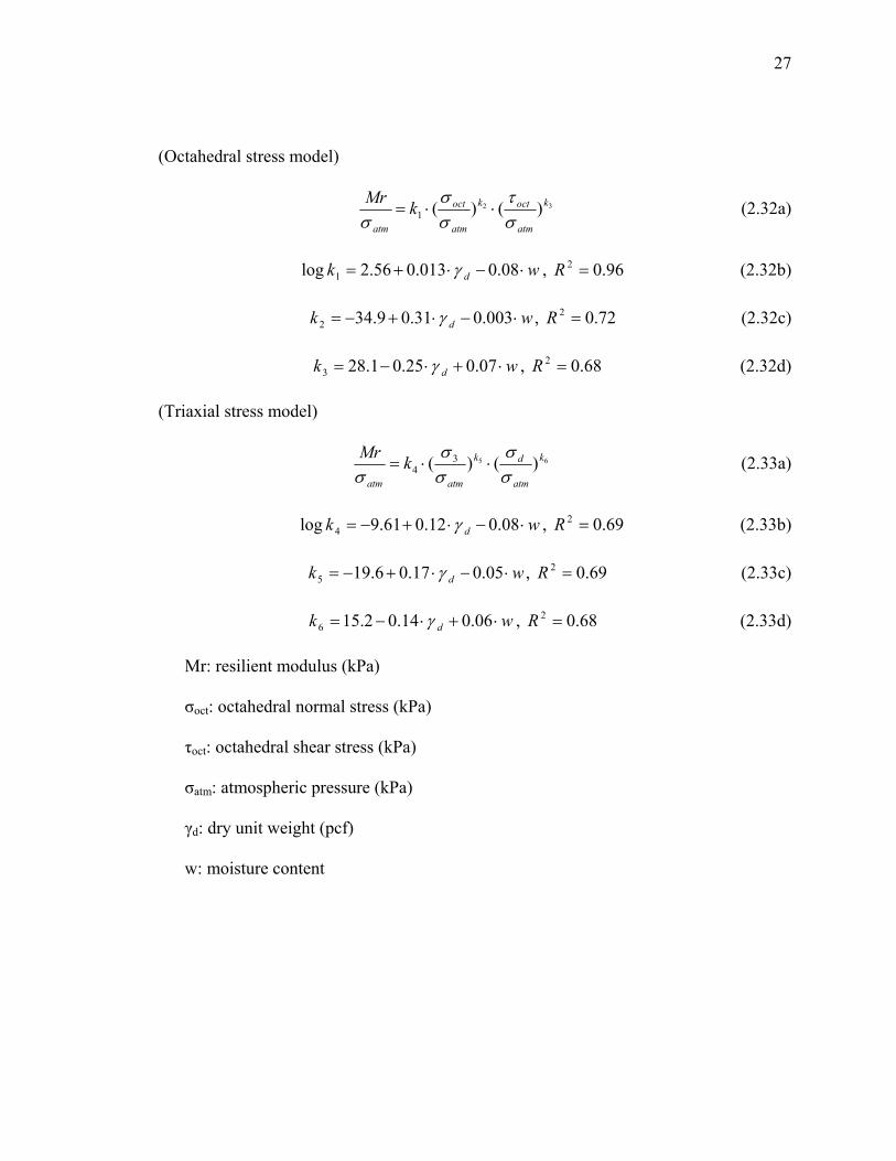
27
(Octahedral stress model)
32 )()(1k
atm
octk
atm
oct
atm
kMrστ
σσ
σ⋅⋅= (2.32a)
wk d ⋅−⋅+= 08.0013.056.2log 1 γ , 96.02 =R (2.32b)
wk d ⋅−⋅+−= 003.031.09.342 γ , 72.02 =R (2.32c)
wk d ⋅+⋅−= 07.025.01.283 γ , 68.02 =R (2.32d)
(Triaxial stress model)
65 )()( 34
k
atm
dk
atmatm
kMrσσ
σσ
σ⋅⋅= (2.33a)
wk d ⋅−⋅+−= 08.012.061.9log 4 γ , 69.02 =R (2.33b)
wk d ⋅−⋅+−= 05.017.06.195 γ , 69.02 =R (2.33c)
wk d ⋅+⋅−= 06.014.02.156 γ , 68.02 =R (2.33d)
Mr: resilient modulus (kPa)
σoct: octahedral normal stress (kPa)
τoct: octahedral shear stress (kPa)
σatm: atmospheric pressure (kPa)
γd: dry unit weight (pcf)
w: moisture content
28
2.5. Permanent Behavior of Subgrades
2.5.1. Permanent Deformations of Cohesive Subgrades
The factors that most affect the permanent deformation of cohesive subgrades are a)
Shear stress level; b) Stress history; c) Thixotropy; d) Frequency of load; e) Moisture
content; f) Freeze-thaw cycles and; g) Overconsolidation ratio.
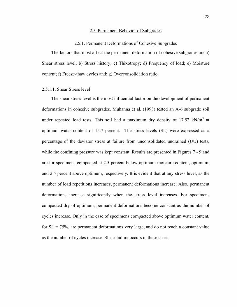
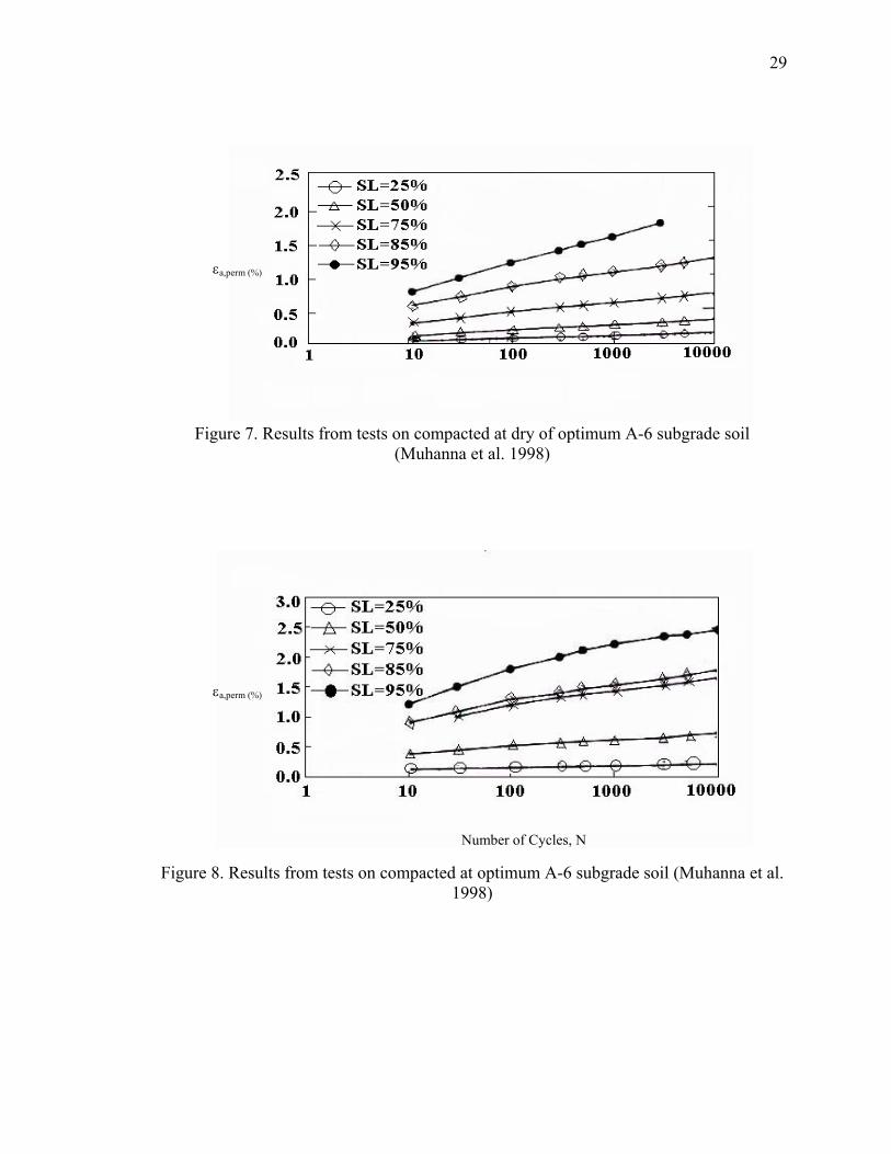
2.5.1.1. Shear Stress level
The shear stress level is the most influential factor on the development of permanent
deformations in cohesive subgrades. Muhanna et al. (1998) tested an A-6 subgrade soil
under repeated load tests. This soil had a maximum dry density of 17.52 kN/m3 at
optimum water content of 15.7 percent. The stress levels (SL) were expressed as a
percentage of the deviator stress at failure from unconsolidated undrained (UU) tests,
while the confining pressure was kept constant. Results are presented in Figures 7 - 9 and
are for specimens compacted at 2.5 percent below optimum moisture content, optimum,
and 2.5 percent above optimum, respectively. It is evident that at any stress level, as the
number of load repetitions increases, permanent deformations increase. Also, permanent
deformations increase significantly when the stress level increases. For specimens
compacted dry of optimum, permanent deformations become constant as the number of
cycles increase. Only in the case of specimens compacted above optimum water content,
for SL = 75%, are permanent deformations very large, and do not reach a constant value
as the number of cycles increase. Shear failure occurs in these cases.
29
Figure 7. Results from tests on compacted at dry of optimum A-6 subgrade soil (Muhanna et al. 1998)
Figure 8. Results from tests on compacted at optimum A-6 subgrade soil (Muhanna et al.
1998)
εa,perm (%)
Number of Cycles, N
εa,perm (%)
30
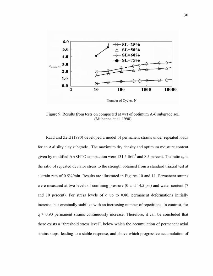
Figure 9. Results from tests on compacted at wet of optimum A-6 subgrade soil (Muhanna et al. 1998)
Raad and Zeid (1990) developed a model of permanent strains under repeated loads
for an A-6 silty clay subgrade. The maximum dry density and optimum moisture content
given by modified AASHTO compaction were 131.5 lb/ft3 and 8.5 percent. The ratio qr is
the ratio of repeated deviator stress to the strength obtained from a standard triaxial test at
a strain rate of 0.5%/min. Results are illustrated in Figures 10 and 11. Permanent strains
were measured at two levels of confining pressure (0 and 14.5 psi) and water content (7
and 10 percent). For stress levels of q up to 0.80, permanent deformations initially
increase, but eventually stabilize with an increasing number of repetitions. In contrast, for
q ≥ 0.90 permanent strains continuously increase. Therefore, it can be concluded that
there exists a “threshold stress level”, below which the accumulation of permanent axial
strains stops, leading to a stable response, and above which progressive accumulation of
Number of Cycles, N
εa,perm (%)

31
axial strains occurs and causes unstable response and ultimately failure. In the case of
Raad and Zeid, the “threshold stress level” was between 0.80 and 0.90. For the tests of
Muhanna et al. (1998), the “threshold stress level” appeared only for specimens
compacted wet of optimum and it was for values of SL between 60 and 75 percent.
The effect of the confining pressure on the tests that Raad and Zeid performed is
very significant. As confining pressure was increased, a stiffening of the soil was
observed, consequently resulting in lower axial strains.
Figure 10. Results from tests on silty clay; left: σ3=0 psi, γd=129.5 lb/ft3, m=7% right: σ3=14.5 psi, γd=129.5 lb/ft3, m=7% (Raad and Zeid 1990)
εa,perm
(%)
εa,perm
(%)
Number of stress repetitions N Number of stress repetitions N

32
Figure 11. Results from tests on silty clay; left: σ3=0 psi, γd=129.5 lb/ft3, m=10% right:
σ3=14.5 psi, γd=129.5 lb/ft3, m=10% (Raad and Zeid 1990)
Raymond et al. (1979) reported the existence of the “threshold stress level” for
Leda clay. This clay is very sensitive and saturated, having a natural water content of
91%, a liquid limit of 66% and a plastic limit of 20%. Drained triaxial tests were
performed under a constant confining pressure of 35 kPa to simulate a typical subgrade
stress. The repeated deviator stress was a percentage of the principal stress difference at
failure, 66 kPa, from drained triaxial tests (at 35 kPa confining pressure). Here, the
“threshold stress level” was about 54 to 60 percent of the deviator stress at failure.
2.5.1.2. Stress history
Monismith et al. (1975) performed a series of undrained triaxial compression tests
on a silty clay (liquid limit = 35, plasticity index = 15). Specimens were prepared at dry
εa,perm
(%)
εa,perm
(%)
Number of stress repetitions N
Number of stress repetitions N
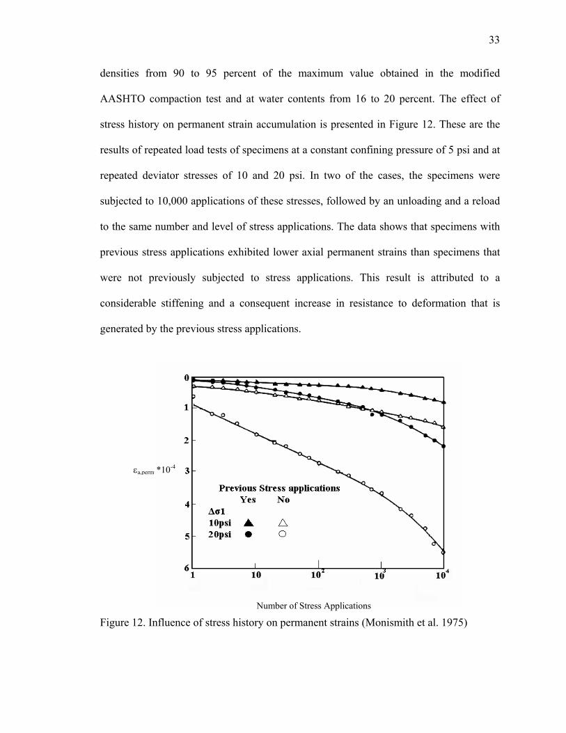
33
densities from 90 to 95 percent of the maximum value obtained in the modified
AASHTO compaction test and at water contents from 16 to 20 percent. The effect of
stress history on permanent strain accumulation is presented in Figure 12. These are the
results of repeated load tests of specimens at a constant confining pressure of 5 psi and at
repeated deviator stresses of 10 and 20 psi. In two of the cases, the specimens were
subjected to 10,000 applications of these stresses, followed by an unloading and a reload
to the same number and level of stress applications. The data shows that specimens with
previous stress applications exhibited lower axial permanent strains than specimens that
were not previously subjected to stress applications. This result is attributed to a
considerable stiffening and a consequent increase in resistance to deformation that is
generated by the previous stress applications.
Figure 12. Influence of stress history on permanent strains (Monismith et al. 1975)
Number of Stress Applications
εa,perm *10-4

34
Seed and Chan (1958) made similar observations when they tested a silty clay
(liquid limit 37 and plastic limit 23). They concluded that this stress stiffening was
probably due to changes in the structural arrangements of the clay particles that
compressed as water dissipated under repeated loads.
2.5.1.3. Thixotropy
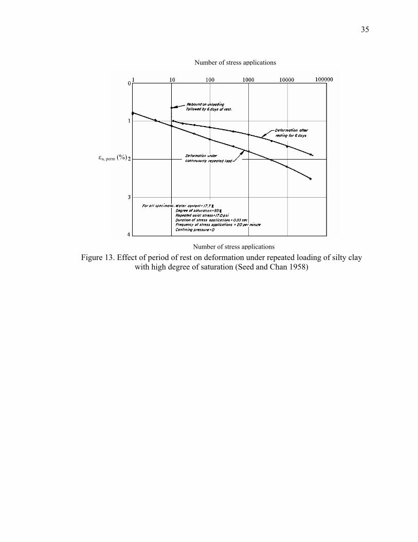
Seed and Chan (1958) investigated the effects of thixotropy (strength gain with time
in saturated clays) on axial strain. This investigation was accomplished by testing
specimens six weeks after compaction, thereby allowing the specimens to gain
considerable thixotropic strength. Figure 13 presents the results for specimens with an
initial degree of saturation of 95 percent. For specimens tested six weeks after
compaction, axial strains were significantly lower than for samples tested immediately
after they were compacted. In contrast, Figure 14 shows the results for specimens at an
initial degree of saturation of 70 percent. The period of rest did not influence the
accumulation of axial strains. Therefore, saturated clay subgrades are affected
significantly by the period of rest. In particular, between long intervals of load
applications, saturated clays regain more thixotropic strength than at short intervals (high
frequencies).
35
Figure 13. Effect of period of rest on deformation under repeated loading of silty clay with high degree of saturation (Seed and Chan 1958)
Number of stress applications
εa, perm (%)
Number of stress applications

36
Figure 14. Effect of period of rest on deformation under repeated loading of silty clay with low degree of saturation (Seed and Chan, 1958)
2.5.1.4. Frequency of load
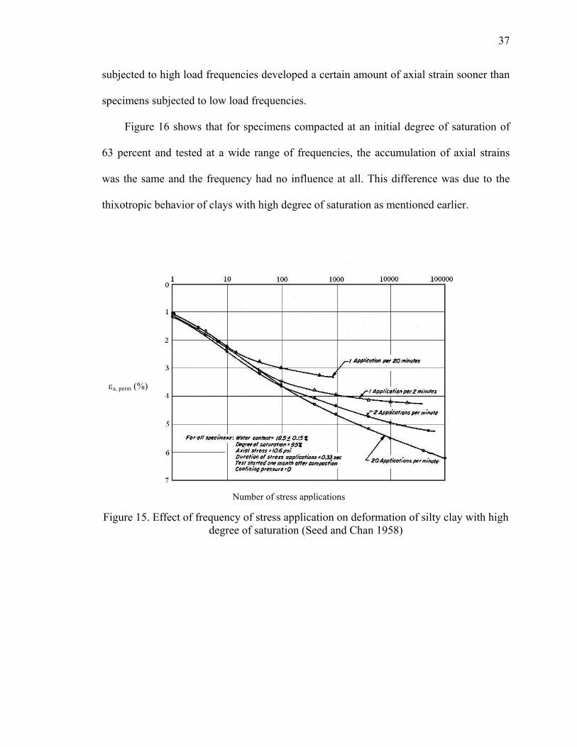
Seed and Chan (1958) thoroughly examined this matter. They found that the
influence of the frequency of load was significant on clays with high degrees of
saturation, which are very thixotropic. Clays with low degrees of saturation (less
thixotropic) were not influenced at all. Figure 15 presents the effect of the load frequency
using stress controlled tests for identical silty clay specimens compacted to an initial
degree of saturation of 95 percent and subjected to repeated stress applications of the
same magnitude and duration, but with varying frequencies. There is large difference in
the number of applications required to cause a certain amount of strain. Specimens
εa, perm (%)
37
subjected to high load frequencies developed a certain amount of axial strain sooner than
specimens subjected to low load frequencies.
Figure 16 shows that for specimens compacted at an initial degree of saturation of
63 percent and tested at a wide range of frequencies, the accumulation of axial strains
was the same and the frequency had no influence at all. This difference was due to the
thixotropic behavior of clays with high degree of saturation as mentioned earlier.
Figure 15. Effect of frequency of stress application on deformation of silty clay with high
degree of saturation (Seed and Chan 1958)
Number of stress applications
εa, perm (%)
Number of stress applications

38
Figure 16. Effect of frequency of stress application on deformation of silty clay with low degree of saturation (Seed and Chan 1958)
2.5.1.5. Moisture content
The influence of moisture content is illustrated in Figures 1 - 4. In all of these
figures, it is apparent that as the moisture content increases, the permanent strains also
increase. Elliott et al. (1999) examined the influence of moisture content on the
permanent deformations of four representative Arkansas cohesive subgrade soils and
found that as moisture content increased (especially for specimens compacted above
optimum), for the same deviator stress, permanent strains increased. This result is
εa, perm (%)
Number of stress applications
39
expected since the presence of water results in a decrease of the resistance to deformation
and therefore strains (irrecoverable, or permanent) consequently increase.
2.5.1.6. Freeze-thaw
Elliott et al. (1999) investigated the effect of freeze-thaw cycles on the permanent
strains. The effect of freeze-thaw was significant, even for one cycle. They reported that
for one freeze-thaw cycle, permanent strains increased up to 100 percent, depending on
the type of subgrade tested.
2.5.1.7. Overconsolidation ratio
Hyde (1974) examined the effect of overconsolidation ratio (OCR) on Keuper Marl
soil. This soil had a liquid limit of 32%, plastic limit of 18% and plasticity index of 14%.
The percentage of clay was found to be 18%. Keuper Marl was subjected to repeated load
tests at a constant confining pressure of 40 kN/m2. The results of these tests for values of
OCR = 4, 10, and 20, showed that as the overconsolidation ratio increased, permanent
strain decreases (for a certain deviator stress). This result is expected since an increasing
OCR leads to an increase in the strength of clays.
2.5.1.8. Models for the permanent strains of cohesive subgrades
Not many models have been suggested to predict the accumulation of permanent
strains in cohesive subgrades under repeated loads. The few models found appear to
reasonably predict the permanent strains for the soil used for the models, but fail to
predict the permanents strains of other soils. These models consider, in general, the

40
number of load repetitions, physical properties and the stress conditions. Several major
models found in the literature are presented.
a. Monismith et al. (1975) proposed the following model
bp NA ⋅=ε (2.34)
εp: permanent strain
N: number of stress applications
A, b: experimentally determined coefficients.
Poulsen and Stubstad (1987) used this model to predict the permanent strains of the
subgrades in six countries and they concluded that it did not represent adequately the
behavior of the investigated soils.
b. Muhanna et al. (1998) proposed the following model
∑ −⋅+=⋅ 0034/7* /)(476.23.1)]/([ wwweSLLog pε (2.35)
Σεp*: accumulated plastic strain (%) at the state of apparent shakedown (shake down can
be defined as the switch of material response from plastic to purely elastic behavior after
a few cycles of loading)
SL: stress level
e: void ratio obtained by T-99 compaction at w
w: molding water content (%)
w0: T-99 optimum moisture content (%)
41
c. Raad and Zeid (1990) suggested the following models for stress levels lower than the
“threshold stress level”.
Nsaq
LL
a
log⋅+=
ε (2.36)
q: stress level
εa: permanent axial strain (%)
αL, sL : material parameters
For stress levels above the “threshold stress level”
ahh
ar ba
qε
ε⋅+
= (2.37a)
NSBb hhh log⋅+= (2.37b)
qr: stress level
εa: permanent axial strain (%)
αh, Bh, Sh : material parameters
2.5.2. Permanent Deformations of Cohesionless Subgrades
Pavements are considered to have failed when the permanent deformations
(irrecoverable deformations) of their components are so large that they cause an
intolerably uneven riding surface, or the recoverable strains induce cracking of the
surfacing material. Thus, the objective of a pavement design should focus on how to limit
the stresses and strains induced by the traffic on the pavement’s materials, so that rutting
(accumulation of permanent deformations) and fatigue failure do not occur. Since
subgrade soils may contribute greatly to the rutting of a pavement, permanent
42
deformations of subgrade soils under repeated loads are important. Traffic is simulated
by triaxial tests, and suitable devices measure permanent deformations. The permanent
deformations of cohesive and cohesionless subgrades will be described in different
sections, due to their differing behaviors.
The factors affecting most permanent deformations of cohesionless subgrades are
the following: a) Stress level; b) Dry unit weight; and c) Moisture content.
2.5.2.1. Stress level
The level of the deviator stress and confining pressure of repeated triaxial tests has
a significant role in the accumulation of permanent strains under repeated loads. Gaskin
et al. (1979) conducted repeated stress tests on a Sydenham sand, which had a Standard
Proctor maximum dry density of 17.7 kN/m3. The confining pressure was kept constant at
35 kPa (5 psi). As seen in Figure 17, the repeated stress was expressed as the ratio X of
the applied stress to the shear strength obtained by a standard triaxial test. For a dry
density of 15.8 kN/m3, this shear strength was 130 kPa. Permanent strains for any stress
level increased until 104 cycles, and at high values of X, permanent strains continued to
increase. In particular, the sample with X = 0.90 failed in shear at about the 500,000th
cycle. The other samples were considered to approach this failure by excessive
deformation. For values of X less than 0.50, permanent strains leveled off and reached a
constant value. At this state, the sand had reached an equilibrium and behaved almost
elastically. As seen in the case of the cohesive subgrades, the existence of a “threshold
stress level” was observed. For the case of the Sydenham sand, this level is
approximately at a value of X = 0.50.
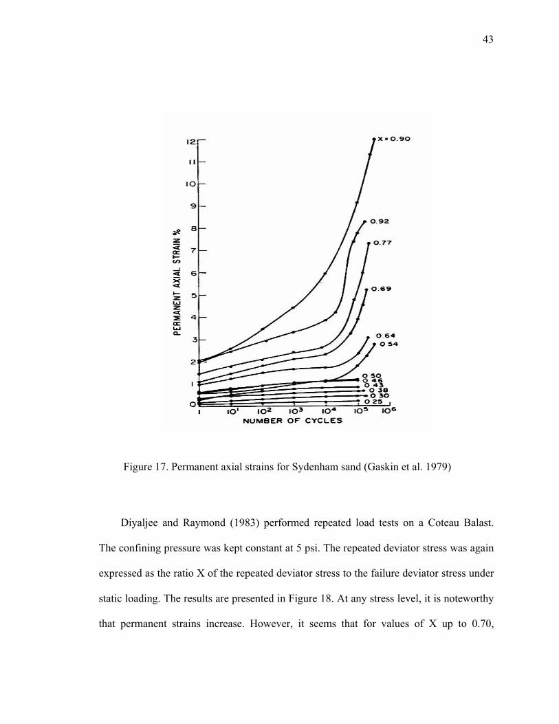
43
Figure 17. Permanent axial strains for Sydenham sand (Gaskin et al. 1979)
Diyaljee and Raymond (1983) performed repeated load tests on a Coteau Balast.
The confining pressure was kept constant at 5 psi. The repeated deviator stress was again
expressed as the ratio X of the repeated deviator stress to the failure deviator stress under
static loading. The results are presented in Figure 18. At any stress level, it is noteworthy
that permanent strains increase. However, it seems that for values of X up to 0.70,

44
permanent strains tend to reach a constant value, while for X = 0.82 permanent strains
continue to increase. Thus, in this case, the “threshold stress level” is estimated at a value
of X between 0.70 and 0.82.
Figure 18. Plastic axial strains for Coteau Balast (Diyaljee and Raymond 1983)
Pumphrey and Lentz (1986) carried out tests on a Florida subgrade sand with a
maximum dry unit weight of 110 pcf and optimum water content of 11 percent
(AASHTO T-180). The repeated deviator stress was a percentage of the peak static soil
strength determined from samples tested at similar dry unit weight and moisture content.
For tests where the confining pressure was constant at 50 psi, they reported (for any of
Number of cycles
εa, perm (%)

45
the tested stress levels) a continuous increase of the permanent strain as the number of
cycles increased. Thus, they did not report a “threshold stress level” for this sand. They
also examined the influence of the confining pressure on the permanent strain as shown
in Figure 19. It was observed that for low stress levels, the effect of the confining
pressure was minor. For the highest stress level, however, permanent strain decreased
with increasing confining pressure. This observation might be the result of aggregate
interlock since the degree of interlock exceeded that observed for the other stress levels.
Notice that for high levels of confining pressure, the difference in the permanent strain
between stress ratios of 0.40 and 0.75 was not significant. This may be explained by the
fact that higher confining pressures led to increasing inter-particle friction, resulting in
less movement, for any stress level.
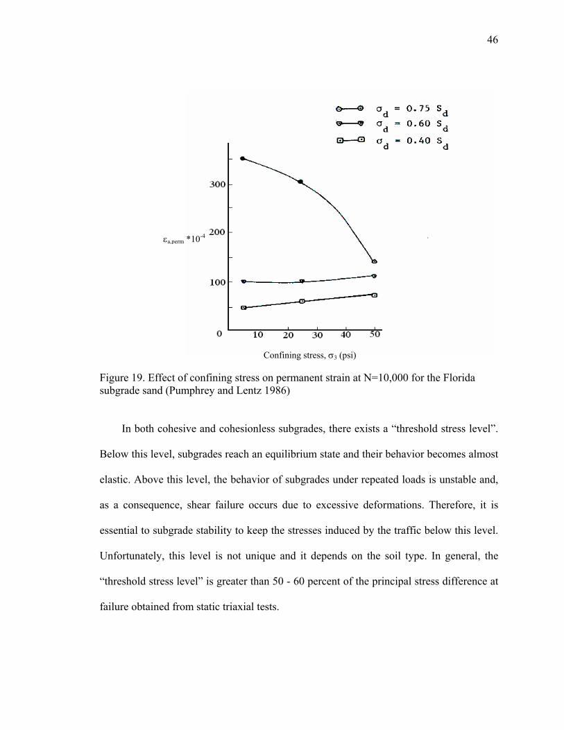
46
Figure 19. Effect of confining stress on permanent strain at N=10,000 for the Florida subgrade sand (Pumphrey and Lentz 1986) In both cohesive and cohesionless subgrades, there exists a “threshold stress level”.
Below this level, subgrades reach an equilibrium state and their behavior becomes almost
elastic. Above this level, the behavior of subgrades under repeated loads is unstable and,
as a consequence, shear failure occurs due to excessive deformations. Therefore, it is
essential to subgrade stability to keep the stresses induced by the traffic below this level.
Unfortunately, this level is not unique and it depends on the soil type. In general, the
“threshold stress level” is greater than 50 - 60 percent of the principal stress difference at
failure obtained from static triaxial tests.
εa,perm *10-4
Confining stress, σ3 (psi)
47
2.5.2.2. Dry unit weight
Pumphrey and Lentz (1986) examined the influence of the dry unit weight on
permanent strain. For samples compacted below and at optimum moisture content, Figure
20 shows the variation of the permanent strain for the 10,000th cycle with the dry unit
weight. As expected, permanent strain decreased as the dry unit weight increased. This
result is reasonable, because with higher dry unit weight the volume of voids becomes
less, resulting in more particle contacts and greater aggregate interlock.
2.5.2.3. Moisture content
As shown in Figure 20, Pumphrey and Lentz (1986) investigated the effects of
moisture content on permanent strain. For samples compacted at optimum moisture
content, permanent strains at the 10,000th cycle are greater than for samples compacted
below optimum. Generally, this is attributed to the fact that less water volume during
compaction allows for a denser soil structure.
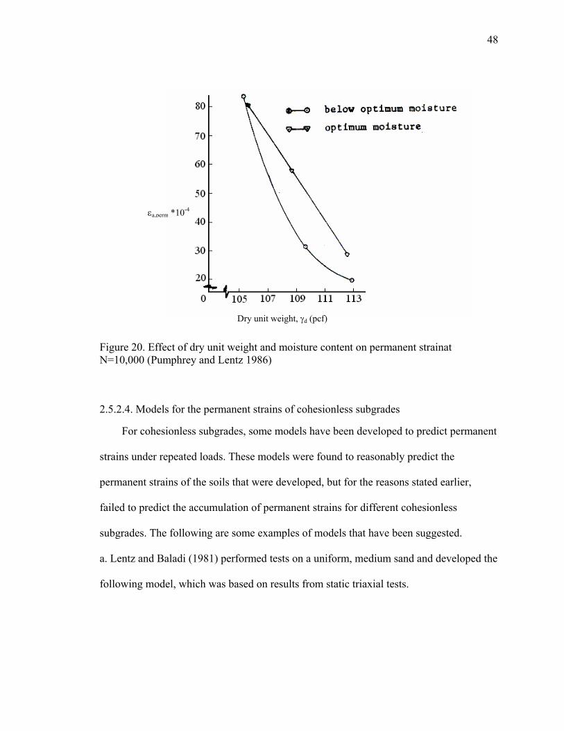
48
Figure 20. Effect of dry unit weight and moisture content on permanent strainat N=10,000 (Pumphrey and Lentz 1986)
2.5.2.4. Models for the permanent strains of cohesionless subgrades
For cohesionless subgrades, some models have been developed to predict permanent
strains under repeated loads. These models were found to reasonably predict the
permanent strains of the soils that were developed, but for the reasons stated earlier,
failed to predict the accumulation of permanent strains for different cohesionless
subgrades. The following are some examples of models that have been suggested.
a. Lentz and Baladi (1981) performed tests on a uniform, medium sand and developed the
following model, which was based on results from static triaxial tests.
εa,perm *10-4
Dry unit weight, γd (pcf)

49
N
Sm
nS
Sd
d
d
d
d
dSp d
ln])(1
)([])1ln([ 15.0
95.0 ⋅⋅−
⋅+−⋅= −
σ
σσ
εε (2.38)
43 10)003769.0809399.0( −⋅⋅+= σn (2.39)
3ln049650.0856355.0 σ⋅+=m (2.40)
εp: permanent strain
ε0.95Sd: static strain at 95 percent of static strength
σd: repeated deviator stress (psi)
Sd: static strength (psi)
n, m: regression constants
σ3: confining pressure (psi)
N: number of cycle
Lekarp and Dawson (1998) mentioned that Sweere used this model for both sands and
granular base course materials and the results were not satisfactory.
b. Diyaljee and Raymond (1983) developed the following general model for the
permanent strain of cohesionless subgrades.
mXnp NeB ⋅⋅= ⋅ε (2.41)
B: value of strain at X = 0 for the first cycle
n, m: experimentally derived parameters
N: number of cycles
X: repeated deviator stress level

50
c. Other models can be found in the paper by Lekarp and Dawson (1998). However, most
of these models were developed for base materials.
51
CHAPTER 3. REVIEW OF THE NEW M-E DESIGN GUIDE
3.1. Introduction
With the release of the Mechanistic-Empirical Design Guide for New and
Rehabilitated Pavement Structures or the M-E Design Guide, highway agencies are
required to implement the new design methodology appropriately. The M-E Design
Guide requires a large number of design inputs related to subgrades, materials,
environment, traffic, drainage, and other pavement elements that need to be considered to
be able to analyze and design pavement (Kim and Zia 2004). In order to fully implement
the M-E Design Guide with greater accuracy, a designer’s knowledge of both design
inputs and pavement performance is required. Successful implementation can be
accomplished by an integrated collaboration between traffic engineers, materials
engineers, geotechnical engineers, and pavement structural engineers (Nantung et al.
2005).
The major objective of this chapter is to provide an extensive review of subgrade
design in the M-E Design Guide. Several design examples for subgrade layers will be
provided in Chapter 8 in accordance with the New Mechanistic-Empirical Design Guide.
3.1.1. Major Differences between the AASHTO Design Guide and M-E Design Guide
TABLE 1 shows the major differences in the design features and philosophies for
subgrades between the existing AASHTO Design Guide and the new M-E Design Guide.

52
In order to design a subgrade with the M-E Design Guide, a pavement designer needs to
use computer software included in the M-E Design Guide (NCHRP 2004) rather than
using the Design Guide book. As designers are required to run the software for pavement
design and the pavement design results and analysis are provided by the software, it is
still necessary to fully understand the principles and features embedded in the software to
achieve rational designs.
In the structural analysis associated with stress and strain developed in the layers
subjected to traffic loadings, the existing AASHTO Design Guide is based on linear
elastic analysis (LEA), while the new M-E Design Guide offers two types of analyses,
LEA and 2-D Finite Element Analysis (FEA). LEA assumes a constant representative
resilient modulus (Mr) for each layer, whereas FEA employs a stress-dependent resilient
modulus for the Level 1 design. According to the NCHRP report on this new M-E Design
Guide (NCHRP 2004), the FEA needs further calibration before it can be implemented.
The M-E Design Guide incorporates unsaturated soil conditions under an
assumption that the subgrade layer will largely be in the unsaturated condition during the
design life period. The unsaturated soil condition is taken into account using the soil
water characteristic curve (SWCC) suggested by Fredlund and Xing (1994). Given the
fact that most geotechnical designs for foundations and slope stability have generally
been done under fully saturated condition of soils for the purpose of conservative design,
the consideration of unsaturated soil conditions is a significant development for a realistic
design of pavement.
Although the existing AASHTO Design Guide recommends the use of Mr monthly
variations, its application was quite limited. The new M-E Design Guide, however,
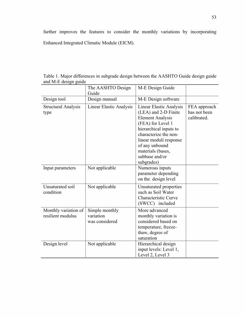
53
further improves the features to consider the monthly variations by incorporating
Enhanced Integrated Climatic Module (EICM).
Table 1. Major differences in subgrade design between the AASHTO Guide design guide and M-E design guide The AASHTO Design
Guide M-E Design Guide
Design tool Design manual M-E Design software Structural Analysis type
Linear Elastic Analysis Linear Elastic Analysis (LEA) and 2-D Finite Element Analysis (FEA) for Level 1 hierarchical inputs to characterize the non-linear moduli response of any unbound materials (bases, subbase and/or subgrades)
FEA approach has not been calibrated.
Input parameters
Not applicable
Numerous inputs parameter depending on the design level
Unsaturated soil condition
Not applicable Unsaturated properties such as Soil Water Characteristic Curve (SWCC) included
Monthly variation of resilient modulus
Simple monthly variation was considered
More advanced monthly variation is considered based on temperature, freeze-thaw, degree of saturation
Design level Not applicable Hierarchical design input levels: Level 1, Level 2, Level 3
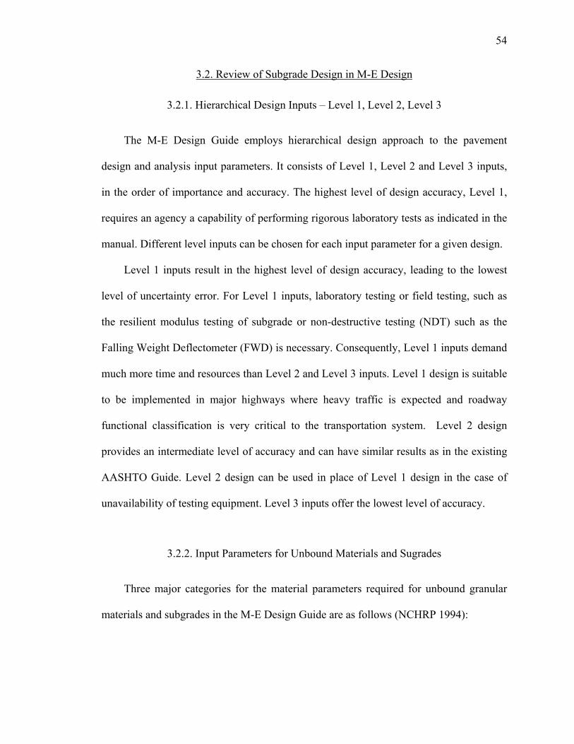
54
3.2. Review of Subgrade Design in M-E Design
3.2.1. Hierarchical Design Inputs – Level 1, Level 2, Level 3
The M-E Design Guide employs hierarchical design approach to the pavement
design and analysis input parameters. It consists of Level 1, Level 2 and Level 3 inputs,
in the order of importance and accuracy. The highest level of design accuracy, Level 1,
requires an agency a capability of performing rigorous laboratory tests as indicated in the
manual. Different level inputs can be chosen for each input parameter for a given design.
Level 1 inputs result in the highest level of design accuracy, leading to the lowest
level of uncertainty error. For Level 1 inputs, laboratory testing or field testing, such as
the resilient modulus testing of subgrade or non-destructive testing (NDT) such as the
Falling Weight Deflectometer (FWD) is necessary. Consequently, Level 1 inputs demand
much more time and resources than Level 2 and Level 3 inputs. Level 1 design is suitable
to be implemented in major highways where heavy traffic is expected and roadway
functional classification is very critical to the transportation system. Level 2 design
provides an intermediate level of accuracy and can have similar results as in the existing
AASHTO Guide. Level 2 design can be used in place of Level 1 design in the case of
unavailability of testing equipment. Level 3 inputs offer the lowest level of accuracy.
3.2.2. Input Parameters for Unbound Materials and Sugrades
Three major categories for the material parameters required for unbound granular
materials and subgrades in the M-E Design Guide are as follows (NCHRP 1994):
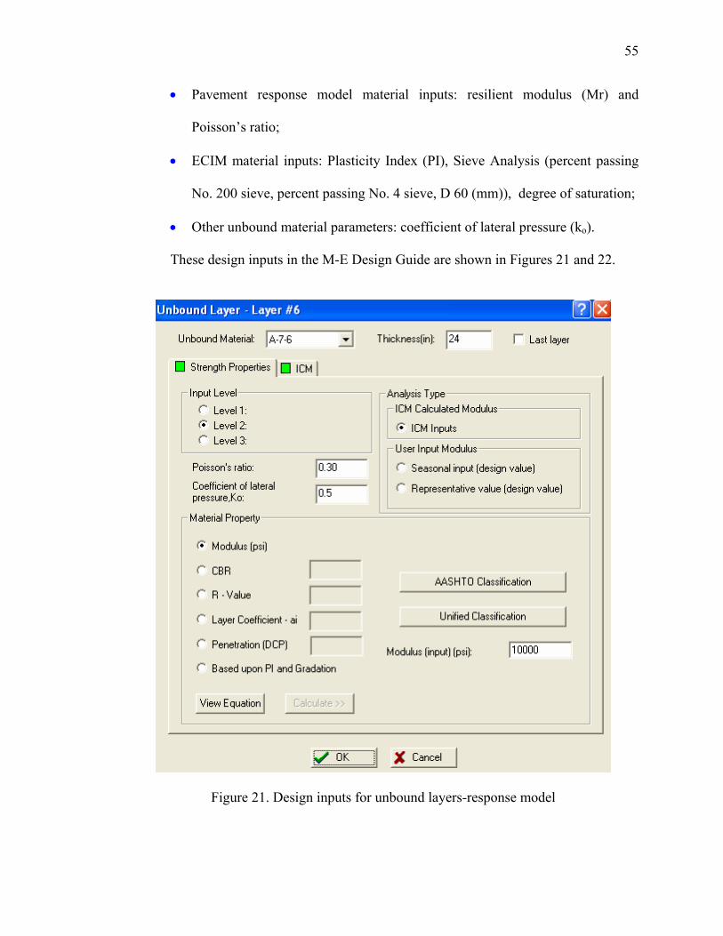
55
• Pavement response model material inputs: resilient modulus (Mr) and
Poisson’s ratio;
• ECIM material inputs: Plasticity Index (PI), Sieve Analysis (percent passing
No. 200 sieve, percent passing No. 4 sieve, D 60 (mm)), degree of saturation;
• Other unbound material parameters: coefficient of lateral pressure (ko).
These design inputs in the M-E Design Guide are shown in Figures 21 and 22.
Figure 21. Design inputs for unbound layers-response model
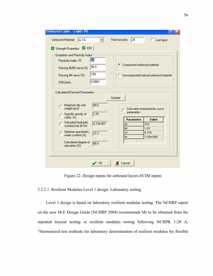
56
Figure 22. Design inputs for unbound layers-ECIM inputs
3.2.2.1. Resilient Modulus-Level 1 design: Laboratory testing
Level 1 design is based on laboratory resilient modulus testing. The NCHRP report
on the new M-E Design Guide (NCHRP 2004) recommends Mr to be obtained from the
repeated triaxial testing or resilient modulus testing following NCHPR 1-28 A,
“Harmonized test methods for laboratory determination of resilient modulus for flexible
57
pavement design” or AASHTO T307, “Determining the resilient modulus of soil and
aggregate materials”.
Many researchers have proposed numerous predictive models to capture the resilient
behavior of soils. The first model for granular materials is the K-θ model (Seed et al.
1967) as follows:
21
kkMr θ= (3. 1)
where k1and k2, = regression coefficients; θ = sum of principal stresses. This model
describes the resilient behavior of soils only as a function of confining stress, and the
effect of deviator stress is not considered.
The another model for cohesive material is the K-σd model is given by:
21
kdkMr σ= (3.2)
where σd is deviator stress. The K-σd model is only associated with the deviator stress.
In order to account for both the confining and deviator stresses, Uzan (1985) suggested a
universal model, which is a more advanced model than both the K-θ model and the K-σd
model. The predicted Mr values can be obtained from the following equation:
32 )()(1k
a
dk
aa pp
pkMr σθ= (3.3)
where, k1, k2, k3, = regression coefficients; θ = sum of principal stresses; pa = reference
pressure = 100 kpa ≈ 1 kgf/cm2 ≈ 2000 psf ≈ 14.5 psi; and σd = deviator stress in the
same unit as pa.
In the M-E design Guide (NCHRP 2004), resilient modulus is predicted using a
similar model to the equation (3.3), as shown below in equation (3.4):

58
32 )1()(1k
a
octk
aa pp
pkMr +=τθ (3.4)
where τoct is the octahedral shear stress. The regression coefficients of the predictive
model can be calculated by performing a regression analysis for the laboratory Mr test
data following AASHTO T 307.
3.2.2.2. Resilient Modulus-Level 2 design: Correlations with other material properties
Level 2 design can be selected when laboratory Mr testing is not available. The
value of resilient modulus can be obtained using typical correlations between resilient
modulus and physical soil properties (dry unit weight, Atterberg limits, specific gravity)
or between resilient modulus and strength properties (i.e., CBR, unconfined compressive
strength). The following correlations are suggested in the M-E Design Guide:
CBR = 28.09 (D60) (3.5)
CBR = 75/(1+0.728 (wPI) (3.6)
CBR=292/DCP1.12 (3.7)
Mr = 2555(CBR)0.64 (3.8)

59
Where D60 = diameter at 60% passing from the grain size distribution (mm); wPI is
weighted plasticity index; CBR = California Bearing Ratio (%); Mr = resilient modulus
(psi); DCP = DCP index (mm/blow). When estimating Mr, the material property is first
related to CBR and then CBR is related to Mr.
For level 2 design, the M-E Design Guide software allows users the following two
options.
• Input a representative value of Mr and use EICM to adjust it for the effect of
seasonal climate (i.e., the effect of freezing, thawing, etc.);
• Input Mr for each month (season) of the year.
3.2.2.2. Resilient Modulus-Level 3 design: Typical Values
For design Level 3, only a typical representative Mr value at optimum moisture
content is required. EICM is used to adjust the representative Mr for the seasonal effect
of climate. Pavement designers may select the representative Mr value without the results
being affected by EICM.
3.2.3. Assumptions Related to Subgrade Compactions in the M-E Design
The M-E Design Guide assumes that the compacted subgrades are compacted near
or at optimum moisture content (OMC) with maximum dry density (the peak point in a
compaction curve) and during the design life of the pavement, they will experience
changes in moisture content without any major variation in dry density (See Figure 23). It
is also assumed that the initial degree of saturation, Sopt (degree of saturation at OMC),
will be in equilibrium depending on drainage properties and environmental conditions
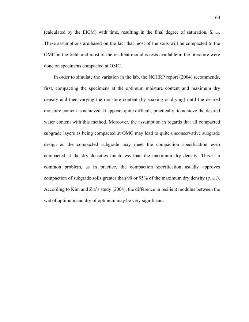
60
(calculated by the EICM) with time, resulting in the final degree of saturation, Sequil.
These assumptions are based on the fact that most of the soils will be compacted to the
OMC in the field, and most of the resilient modulus tests available in the literature were
done on specimens compacted at OMC.
In order to simulate the variation in the lab, the NCHRP report (2004) recommends,
first, compacting the specimens at the optimum moisture content and maximum dry
density and then varying the moisture content (by soaking or drying) until the desired
moisture content is achieved. It appears quite difficult, practically, to achieve the desired
water content with this method. Moreover, the assumption in regards that all compacted
subgrade layers as being compacted at OMC may lead to quite unconservative subgrade
design as the compacted subgrade may meet the compaction specification even
compacted at the dry densities much less than the maximum dry density. This is a
common problem, as in practice, the compaction specification usually approves
compaction of subgrade soils greater than 90 or 95% of the maximum dry density (γdmax).
According to Kim and Zia’s study (2004), the difference in resilient modulus between the
wet of optimum and dry of optimum may be very significant.
61
Figure 23. Variation in moisture contents for the compacted subgrade
Moisture content (%)
γd
γd max
As-compacted (OMC) In equilibrium (M-E Design)
0.95γd max
Dry Wet Z.A.V curve
62
3.2.4. Climatic and Environmental Effects in the M-E Design
Moisture and temperature are two key factors that significantly affect the pavement
layer and subgrade properties and its load carrying capacity. Effects of these factors on
resilient modulus are considered in the M-E Design Guide.
3.2.4.1. The Enhanced Integrated Climatic Model (EICM)
In the M-E Design Guide, variation in temperature and moisture in subgrade soils
are considered throughout the design life through the Enhanced Integrated Climatic
Model (EICM). The EICM is composed of the following three components (NCHRP
2004):
• The Climatic-Materials-Structure Model (CMS Model)
• The CRREL Frost-Heave and Thaw Settlement Model (CRREL Model)
• The Infiltration and Drainage Model (ID Model)
Input parameters required by the climatic model are general information, such as
weather related information, ground water related information, drainage and surface
properties, pavement structure and material characteristics. The EICM calculates
temperature, resilient modulus adjustment factors (FF, FR, FU), pore water pressure, frost
and thaw depth, frost heave, and drainage performance over the design period. It is noted
in the M-E Design that one of the important factors required from EICM is a set of
adjustment factors for unbound material layers that account for the effect of

63
environmental parameters and conditions such as changes in moisture content, freezing,
thawing, and recovery from thawing. The environmental factor, Fenv is a composite factor,
which could generally represent a weighted average of the factors appropriate for
possible conditions.
• Frozen: frozen material - FF (factor for frozen material, calculated based on
the temperature)
• Recovering: thawed material that is recovering to its state before freezing
occurred- FR (factor of recovering materials)
• Unfrozen/ fully recovered/normal: for materials that were never frozen or are
fully recovered- FU (factor for unfrozen materials)
Since the resilient modulus in the M-E Design Guide depends on stress, moisture
and free/thaw effects, the values of the resilient modulus at any location and time within a
given pavement structure are calculated as a function of those factors. The resilient
modulus Mr at any time or location is then expressed as follows:
optenv MrFMr ×= (3.9)
where Fenv is an adjustment factor and Mropt is the resilient modulus at optimum
conditions (maximum dry density and optimum moisture content) and any state of stress.
The EICM accounts for unsaturated soil conditions based on the soil-water
characteristic curve (SWCC) suggested by Fredlund and Xing (1994), saturated and
unsaturated hydraulic conductivity, a climatic database containing hourly data from 800
weather stations across the United States for sunshine, rainfall, wind speed, air

64
temperature and relative humidity (NCHRP 2004). The SWCC is generally used in
unsaturated soil mechanics and defined as variation of water storage capacity within the
macro-and micro-pores of a soil, with respect to suction. This relationship is generally
plotted as variation of water content (gravimetric, volumetric, or degree of saturation)
with soil suction. The SWCC is used to calculate the degree of saturation in equilibrium,
Sequil as given by:
ff
cb
f
equil
ahEXP
hCS
⎥⎥
⎦
⎤
⎢⎢
⎣
⎡
⎥⎥
⎦
⎤
⎢⎢
⎣
⎡
⎟⎟⎠
⎞⎜⎜⎝
⎛+
×=
)1(ln
1)( ,
⎟⎟⎠
⎞⎜⎜⎝
⎛ ×+
⎟⎟⎠
⎞⎜⎜⎝
⎛+
−=
r
r
h
hh
hC51045.11ln
1ln1)( (3.10)
where h = distance from the point in question to ground water table and af, bf, cf, and
hr = input parameters obtained from regression analyses.
3.2.4.2. Resilient modulus as function of soil moisture
Moisture content is an important factor affecting resilient behavior of soils.
Generally, for a given soil with the same dry density, the higher the moisture content, the
lower the resilient modulus. The M-E Design Guide incorporates a predictive equation
within the EICM to predict changes in modulus due to changes in moisture. The resilient
modulus as a function of soil moisture in the M-E Design Guide is as follows:
))((ln1log
optmopt SSk
abEXP
abaMrMr
−+−
+
−+= (3.11)
65
where, Mr/Mropt = resilient modulus ratio; Mr is the resilient modulus at a given time and
Mropt is the resilient modulus at the optimum moisture content; a = minimum of log
(Mr/Mropt); b = maximum of log (Mr/Mropt); km = regression parameter; (S – Sopt) =
variation in degree of saturation expressed in decimal.
The M-E Design Guide (NCHRP 2004) suggests that the modulus ratio, Mr/Mropt, is
in the range of 2 to 0.5 for coarse-grained soils, while it is between 2.5 to 0.5 for fine-
grained soils. This means that the fine-grained soils are more influenced by the moisture
content than the coarse-grained soils. Generally, the degree of saturation of subgrades
(especially for fine-grained subgrades) increases with time, the resilient modulus will
decrease over the design period due to the increase in moisture content and reach the
minimum resilient modulus. It is noted that Mr values of Indiana subgrade soils were
reported by Kim and Zia (2004) for a confining stress of 2 psi and a deviator stress of 6
psi. The average Mr/Mropt is 0.28, which is considerably lower than 0.5.
3.2.4.3. Resilient Modulus for Frozen/ Thawed Unbound Materials
In the M-E Design Guide, a significant literature search was done to study the
behavior of unbound materials under freezing/thawing conditions. It presents absolute
values of moduli for frozen material, termed Mrfrz and the ratio of Mr just after thawing,
termed Mrmin, to the Mr of natural, unfrozen material, termed Mrunfrz. The ratio is used as
a reduction factor, termed RF. Since some of the data from the literature produced RF
values based on Mrunfrz as a reference and some were based on Mropt as a reference, it
adopted a conservative interpretation of using the smaller of Mrunfrz and Mropt as a
reference. The definitions are as follows:

66
Mrfrz = Mrmax = Mr for frozen material
Mrunfrz = the normal Mr for unfrozen material
Mrmin = Mr just after thawing
RF = modulus reduction factor = Mrmin/ smaller of (Mrunfrz, Mropt)
The M-E Design Guide recommends Mrfrz, ave = 3,000,000 psi for coarse grained
materials, Mrfrz_ave = 2,000,000 psi for fine grained silt and silty sands, Mrfrz_ave =
1,000,000 psi, as a conservative value for clays. Note that Lee et al. (1993) recommends
resilient modulus ranging from 27000 to 46000 psi for typical Indiana soils based on their
test results, which are considerably smaller values than Mrfrz_ave.
3.2.5. Summary
With the advent of the new M-E Design Guide, highway agencies are encouraged to
implement an advanced design following its philosophies. As part of implementation of
the M-E Design Guide, the present study reviews the features embedded in this new
design guide for unbound materials, especially subgrades.
The following can be summarized:
• The M-E Design Guide assumes that the subgrade is compacted to optimum
moisture content, leading to unconservative design. In order to ensure a

67
conservative design for subgrades, the use of the average moisture content
between OMC and wet of optimum (95% compaction) is recommended;
• When laboratory testing for evaluating thawed Mr is not available, the use of
Mr for wet of optimum would be reasonable;
• Caution needs to be taken to use the unconservative frozen Mr value
suggested in M-E Design Guide.
In characterizing subgrade in Indiana, Mr testing program for both design inputs
Level 2 and Level 1 are desirable. In addition, the following initiatives will be conducted
to enhance characterization of subgrade:
• Mr monthly variation laboratory testing to simulate freeze-thaw in the
subgrade;
• Mr long term laboratory simulation to consider permanent strain for pavement
rehabilitation;
• Correlation between Mr and FWD data for non-destructive testing evaluation;
• Laboratory evaluation on unsaturated soil properties such as soil water
characteristic curve (SWCC).
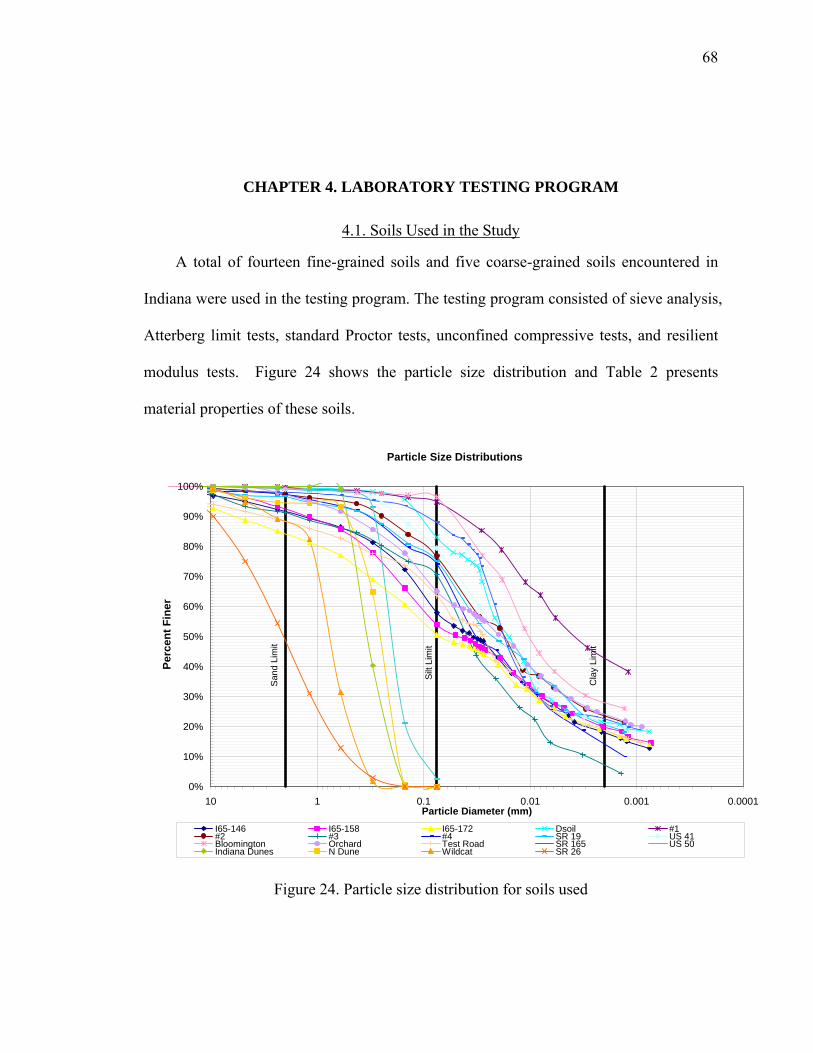
68
CHAPTER 4. LABORATORY TESTING PROGRAM
4.1. Soils Used in the Study
A total of fourteen fine-grained soils and five coarse-grained soils encountered in
Indiana were used in the testing program. The testing program consisted of sieve analysis,
Atterberg limit tests, standard Proctor tests, unconfined compressive tests, and resilient
modulus tests. Figure 24 shows the particle size distribution and Table 2 presents
material properties of these soils.
Particle Size Distributions
Sand
Lim
it
Silt
Lim
it
Cla
y Li
mit
0%
10%
20%
30%
40%
50%
60%
70%
80%
90%
100%
0.00010.0010.010.1110Particle Diameter (mm)
Perc
ent F
iner
I65-146 I65-158 I65-172 Dsoil #1 #2 #3 #4 SR 19 US 41Bloomington Orchard Test Road SR 165 US 50Indiana Dunes N Dune Wildcat SR 26
Figure 24. Particle size distribution for soils used
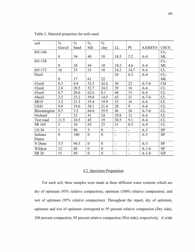
69
Table 2. Material properties for soils used
soil % Gravel
% Sand
% Silt
% clay LL PI AASHTO USCS
I65-146 8 34 40 18 18.5 5.2 A-4
CL-ML
I65-158 8 38 44 10 18.2 4.6 A-4
CL-ML
I65-172 16 33 33 18 24.2 14.7 A-6 CL Dsoil
0 17 61 22 26 6.2 A-4 CL-
ML #1soil 0.3 4.8 52.3 42.6 50 23 A-7-6 CH #2soil 2.6 20.5 52.7 24.2 39 16 A-6 CL #3soil 8.7 20.6 62.6 8.1 40 15 A-6 CL #4soil 2.5 23.2 59.8 14.5 43 21 A-7-6 CL SR19 3.2 21.5 55.4 19.9 33 16 A-6 CL US41 0.9 19.6 58.1 21.4 28 9 A-4 CL Bloomington 0.3 3.2 60.6 35.9 46 26 A-7-6 CL Orchard 3 32 41 24 29.8 12 A-6 CL Test road 11.5 24.5 45 19 30.5 9.1 A-4 CL SR 165 2 10 65 23 31 8.5 A-4 CL US 50 1 96 3 0 - - A-3 SP Indiana Dunes
0 100 0 0 - - A-3 SP
N Dune 5.5 94.5 0 0 - - A-3 SP Wildcat 12 88 0 0 - - A-1-b SP SR 26 51 49 0 0 - - A-1-b GP
4.2. Specimen Preparation
For each soil, three samples were made at three different water contents which are
dry of optimum (95% relative compaction), optimum (100% relative compaction), and
wet of optimum (95% relative compaction). Throughout the report, dry of optimum,
optimum and wet of optimum correspond to 95 percent relative compaction (Dry side),
100 percent compaction, 95 percent relative compaction (Wet side), respectively. A wide
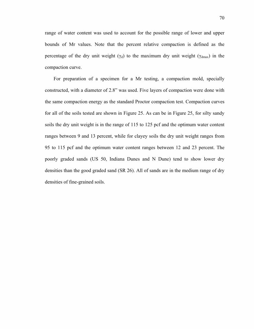
70
range of water content was used to account for the possible range of lower and upper
bounds of Mr values. Note that the percent relative compaction is defined as the
percentage of the dry unit weight (γd) to the maximum dry unit weight (γdmax) in the
compaction curve.
For preparation of a specimen for a Mr testing, a compaction mold, specially
constructed, with a diameter of 2.8” was used. Five layers of compaction were done with
the same compaction energy as the standard Proctor compaction test. Compaction curves
for all of the soils tested are shown in Figure 25. As can be in Figure 25, for silty sandy
soils the dry unit weight is in the range of 115 to 125 pcf and the optimum water content
ranges between 9 and 13 percent, while for clayey soils the dry unit weight ranges from
95 to 115 pcf and the optimum water content ranges between 12 and 23 percent. The
poorly graded sands (US 50, Indiana Dunes and N Dune) tend to show lower dry
densities than the good graded sand (SR 26). All of sands are in the medium range of dry
densities of fine-grained soils.
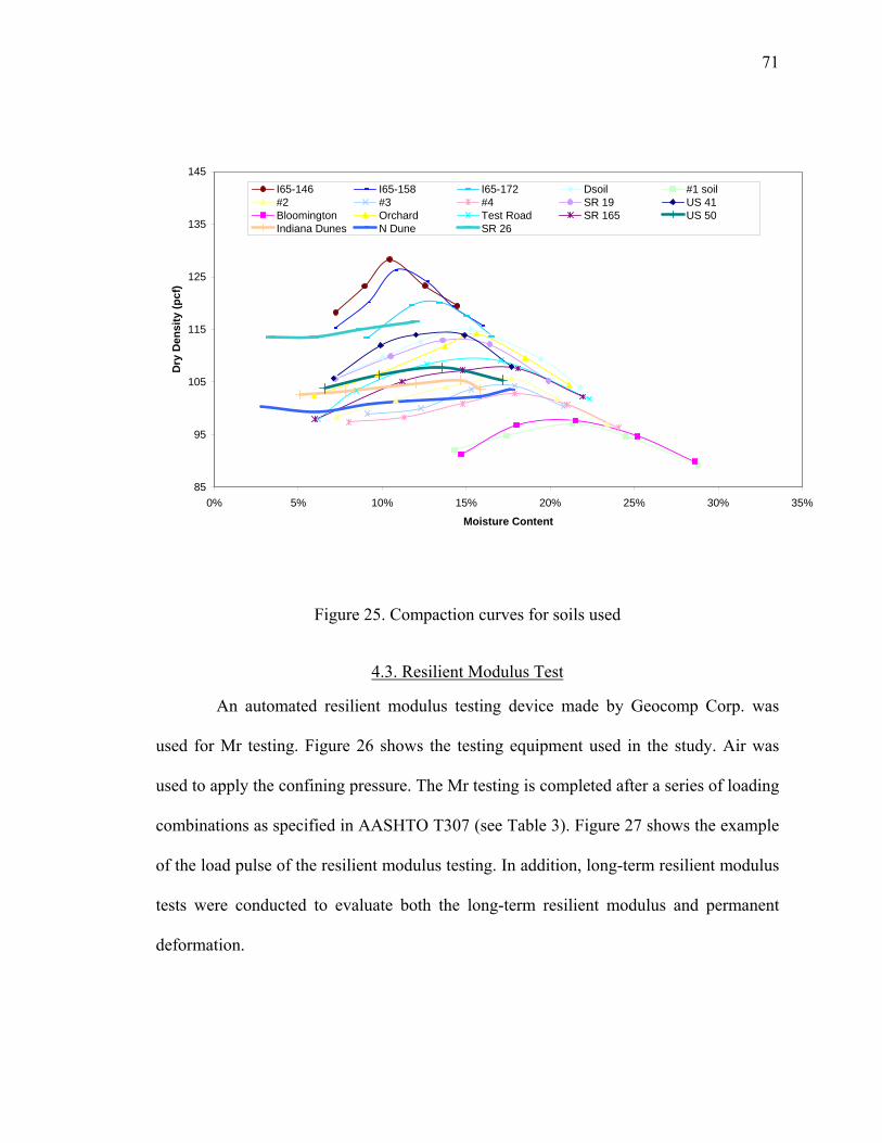
71
85
95
105
115
125
135
145
0% 5% 10% 15% 20% 25% 30% 35%
Moisture Content
Dry
Den
sity
(pcf
)I65-146 I65-158 I65-172 Dsoil #1 soil#2 #3 #4 SR 19 US 41Bloomington Orchard Test Road SR 165 US 50Indiana Dunes N Dune SR 26
Figure 25. Compaction curves for soils used
4.3. Resilient Modulus Test
An automated resilient modulus testing device made by Geocomp Corp. was
used for Mr testing. Figure 26 shows the testing equipment used in the study. Air was
used to apply the confining pressure. The Mr testing is completed after a series of loading
combinations as specified in AASHTO T307 (see Table 3). Figure 27 shows the example
of the load pulse of the resilient modulus testing. In addition, long-term resilient modulus
tests were conducted to evaluate both the long-term resilient modulus and permanent
deformation.
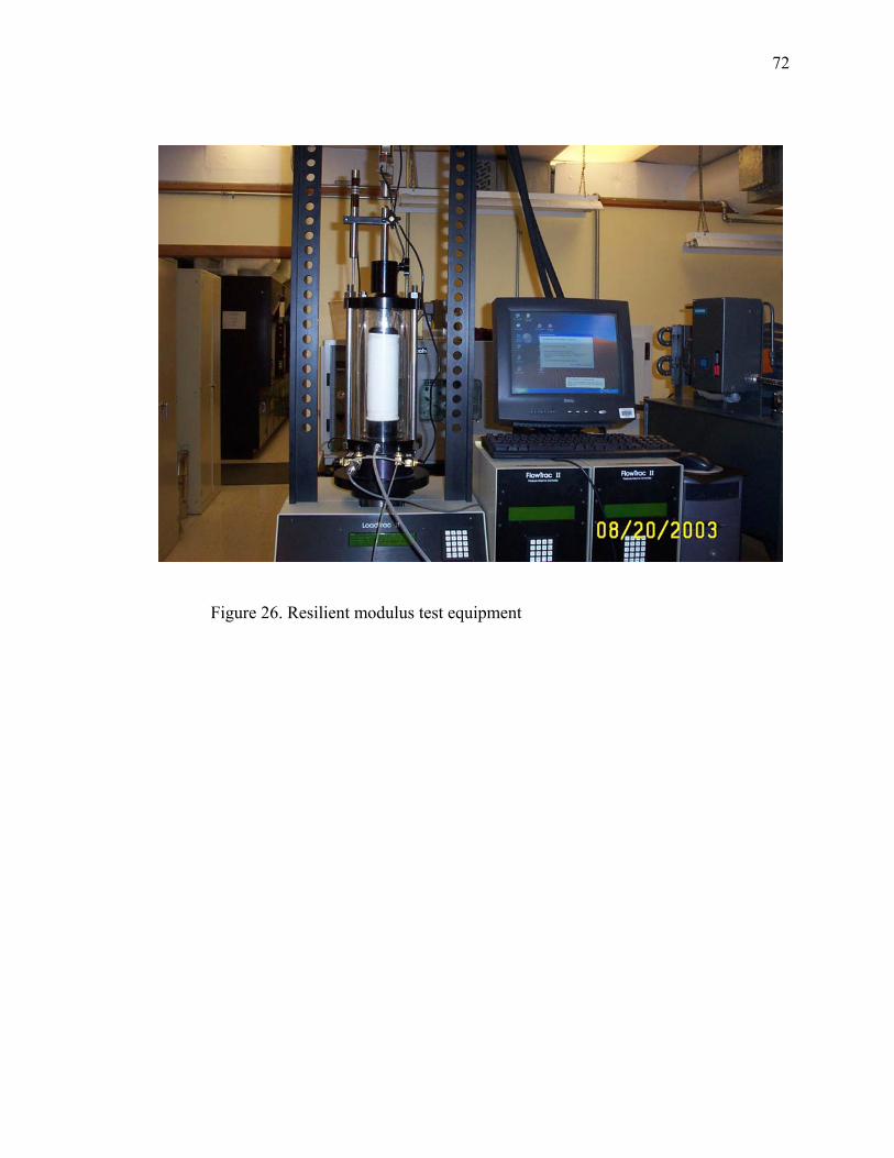
72
Figure 26. Resilient modulus test equipment
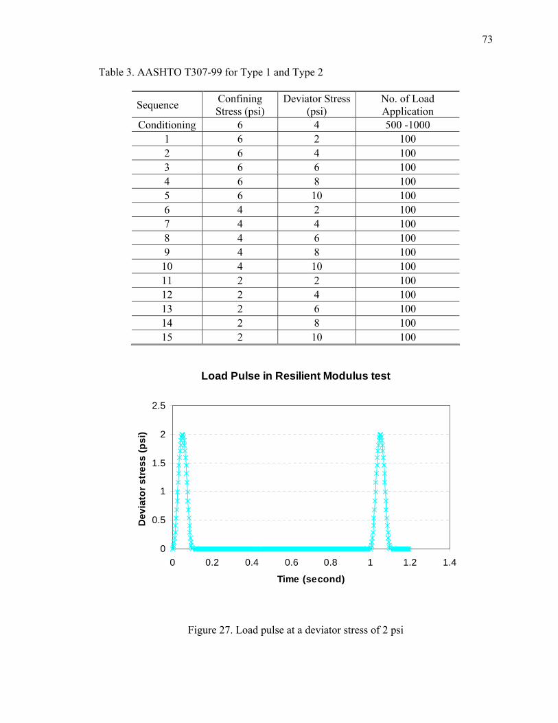
73
Table 3. AASHTO T307-99 for Type 1 and Type 2
Sequence Confining Stress (psi)
Deviator Stress (psi)
No. of Load Application
Conditioning 6 4 500 -1000 1 6 2 100 2 6 4 100 3 6 6 100 4 6 8 100 5 6 10 100 6 4 2 100 7 4 4 100 8 4 6 100 9 4 8 100 10 4 10 100 11 2 2 100 12 2 4 100 13 2 6 100 14 2 8 100 15 2 10 100
Load Pulse in Resilient Modulus test
0
0.5
1
1.5
2
2.5
0 0.2 0.4 0.6 0.8 1 1.2 1.4
Time (second)
Dev
iato
r str
ess
(psi
)
Figure 27. Load pulse at a deviator stress of 2 psi

74
4.4. Dynamic Cone Penetration (DCP) Tests
The dynamic cone penetration test used in this experiment was performed in the
laboratory to produce any possible correlations between the DCP index and the resilient
modulus. Specimens were compacted in a 6” diameter and 9” high mold (CBR mold)
using the standard Proctor compaction energy, requiring significant amount of soil and
time consuming compaction effort. This was achieved using 8 soil layers and 37 blows
using a standard proctor hammer on each layer. The DCPT was performed on dry and
OMC samples for five soils (Bloomington, Orchard, Test Road, Exit 172, SR 165). It was
not possible to perform the test on wet soil samples, as the weight of the apparatus caused
the cone to penetrate the soil, giving the wet samples a penetration index of infinity. The
other soils were penetrated to an approximate depth of 6” to reduce the effect of
confinement from the bottom of the mold on the results.

75
CHAPTER 5. DISCUSSION OF THE TEST RESULTS
5.1. Resilient modulus test
5.1.1. Results of Resilient Modulus Test on Cohesive Subgrade Soils
5.1.1.1. Multi-layered Elastic Analyses
In order to evaluate the range of confining and deviator stresses generated in the
subgrade, several multilayered elastic analyses were performed on four typical pavement
cross-sections (See Kim 2002). The cross-sections consist of a 4 to 6 inches of asphalt
layer, a 6 to 8 inches of base layer and a 12 inches of compacted clay or sand subgrade
layer followed by a infinite layer. A single axle load of 18 kips with an inflation pressure
of 100 psi was applied to the surface of the pavement. For an extreme scenario, a super
single tire loading with an inflation pressure of 125 psi (Kim 2002) was also applied.
Figure 28 shows the evaluation points in the subgrade layer. Analysis results showed that
the confining stresses induced in the subgrades for four typical Indiana cross-sections
range from 2 psi to 6 psi and deviator stresses range from 2 to 18 psi. One of the analyses
on the deviator stresses induced in the subgrade is shown in Figure 29. The 15 psi would
be the highest deviator stresses that the subgrade ever experiences (except for supersingle
load). Note that the highest deviator stress is a little higher than 10 psi specifed in
AASHTO T 307.
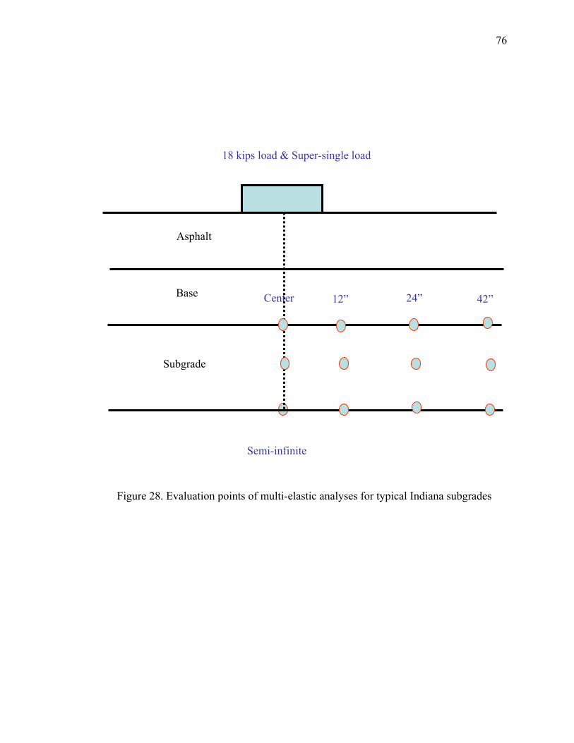
76
Figure 28. Evaluation points of multi-elastic analyses for typical Indiana subgrades
Asphalt
Base
Subgrade
12” 24” 42” Center
Semi-infinite
18 kips load & Super-single load
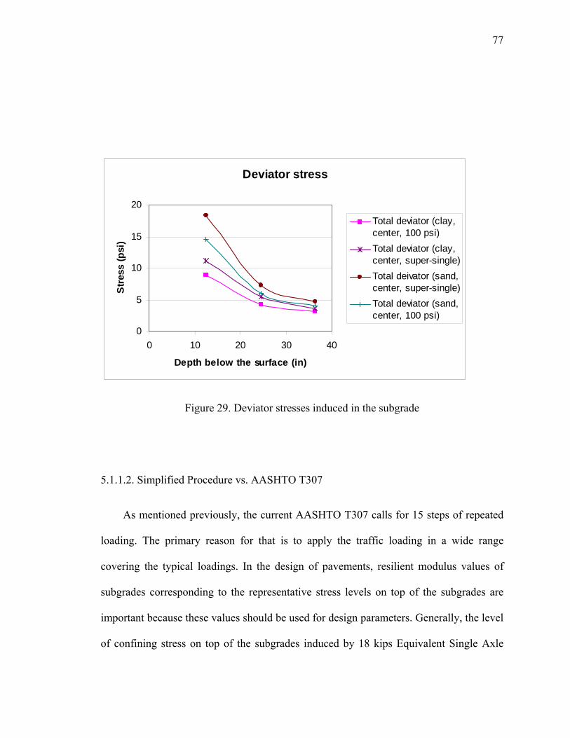
77
Deviator stress
0
5
10
15
20
0 10 20 30 40
Depth below the surface (in)
Stre
ss (p
si)
Total deviator (clay,center, 100 psi)Total deviator (clay,center, super-single)Total deivator (sand,center, super-single)Total deviator (sand,center, 100 psi)
Figure 29. Deviator stresses induced in the subgrade
5.1.1.2. Simplified Procedure vs. AASHTO T307
As mentioned previously, the current AASHTO T307 calls for 15 steps of repeated
loading. The primary reason for that is to apply the traffic loading in a wide range
covering the typical loadings. In the design of pavements, resilient modulus values of
subgrades corresponding to the representative stress levels on top of the subgrades are
important because these values should be used for design parameters. Generally, the level
of confining stress on top of the subgrades induced by 18 kips Equivalent Single Axle
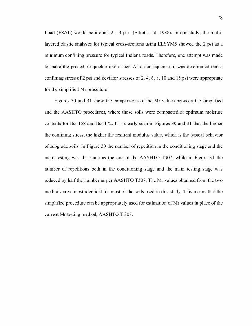
78
Load (ESAL) would be around 2 - 3 psi (Elliot et al. 1988). In our study, the multi-
layered elastic analyses for typical cross-sections using ELSYM5 showed the 2 psi as a
minimum confining pressure for typical Indiana roads. Therefore, one attempt was made
to make the procedure quicker and easier. As a consequence, it was determined that a
confining stress of 2 psi and deviator stresses of 2, 4, 6, 8, 10 and 15 psi were appropriate
for the simplified Mr procedure.
Figures 30 and 31 show the comparisons of the Mr values between the simplified
and the AASHTO procedures, where those soils were compacted at optimum moisture
contents for I65-158 and I65-172. It is clearly seen in Figures 30 and 31 that the higher
the confining stress, the higher the resilient modulus value, which is the typical behavior
of subgrade soils. In Figure 30 the number of repetition in the conditioning stage and the
main testing was the same as the one in the AASHTO T307, while in Figure 31 the
number of repetitions both in the conditioning stage and the main testing stage was
reduced by half the number as per AASHTO T307. The Mr values obtained from the two
methods are almost identical for most of the soils used in this study. This means that the
simplified procedure can be appropriately used for estimation of Mr values in place of the
current Mr testing method, AASHTO T 307.
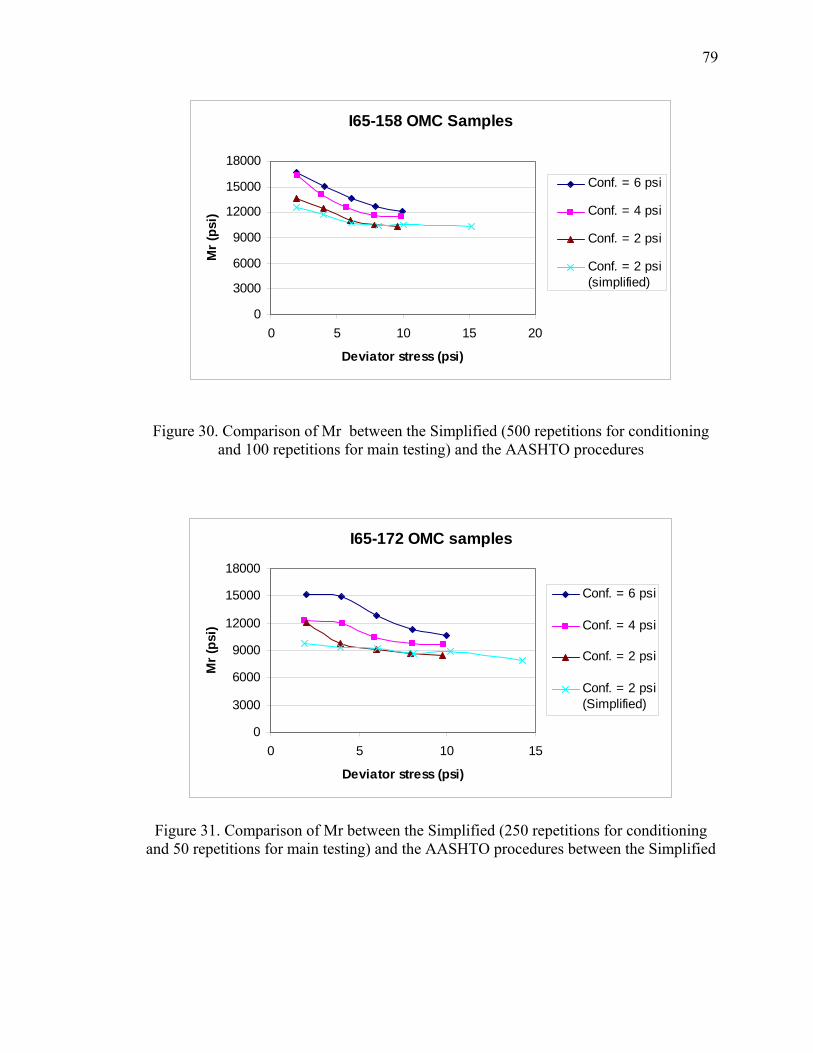
79
I65-158 OMC Samples
0
3000
6000
9000
12000
15000
18000
0 5 10 15 20
Deviator stress (psi)
Mr
(psi
)
Conf. = 6 psi
Conf. = 4 psi
Conf. = 2 psi
Conf. = 2 psi(simplified)
Figure 30. Comparison of Mr between the Simplified (500 repetitions for conditioning and 100 repetitions for main testing) and the AASHTO procedures
I65-172 OMC samples
0
3000
6000
9000
12000
15000
18000
0 5 10 15
Deviator stress (psi)
Mr (
psi)
Conf. = 6 psi
Conf. = 4 psi
Conf. = 2 psi
Conf. = 2 psi(Simplified)
Figure 31. Comparison of Mr between the Simplified (250 repetitions for conditioning and 50 repetitions for main testing) and the AASHTO procedures between the Simplified
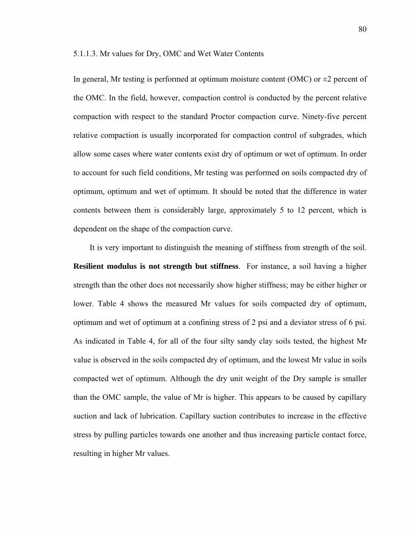
80
5.1.1.3. Mr values for Dry, OMC and Wet Water Contents
In general, Mr testing is performed at optimum moisture content (OMC) or ±2 percent of
the OMC. In the field, however, compaction control is conducted by the percent relative
compaction with respect to the standard Proctor compaction curve. Ninety-five percent
relative compaction is usually incorporated for compaction control of subgrades, which
allow some cases where water contents exist dry of optimum or wet of optimum. In order
to account for such field conditions, Mr testing was performed on soils compacted dry of
optimum, optimum and wet of optimum. It should be noted that the difference in water
contents between them is considerably large, approximately 5 to 12 percent, which is
dependent on the shape of the compaction curve.
It is very important to distinguish the meaning of stiffness from strength of the soil.
Resilient modulus is not strength but stiffness. For instance, a soil having a higher
strength than the other does not necessarily show higher stiffness; may be either higher or
lower. Table 4 shows the measured Mr values for soils compacted dry of optimum,
optimum and wet of optimum at a confining stress of 2 psi and a deviator stress of 6 psi.
As indicated in Table 4, for all of the four silty sandy clay soils tested, the highest Mr
value is observed in the soils compacted dry of optimum, and the lowest Mr value in soils
compacted wet of optimum. Although the dry unit weight of the Dry sample is smaller
than the OMC sample, the value of Mr is higher. This appears to be caused by capillary
suction and lack of lubrication. Capillary suction contributes to increase in the effective
stress by pulling particles towards one another and thus increasing particle contact force,
resulting in higher Mr values.
81
Table 4. Measured Mr values for Dry, OMC and Wet samples (σc = 2 psi, σd = 6 psi )
Mr values (psi) Soil Type and Source Dry OMC Wet
I65-146 13,641 3,327 2,946 I65-158 15,867 11,104 3,970 I65-172 16,710 9,631 2,605
Silty sandy clay soils
Dsoil 12,278 9,310 1,996 #1soil 16,617 12,587 7,235 #2soil 13,444 17,563 2,430 #3soil 14,439 18,813 1,633 #4soil 11,440 10,697 1,717 SR19 25,047 22,896 1,884 US41 24,209 14,489 2,376 Bloomington 13,725 13,488 2,026 Orchard 12,587 14,322 2,913 Test road 13,857 12,523 3,325
Clay soils
SR 165 11,276 9,409 2,405
5.1.1.4. Silty Sandy Clay soils
Figures 32-35 present the unconfined compressive test results for OMC, Dry and
Wet samples for I65-146, I65-158, I65-172 and Dsoil, respectively. Unconfined
compressive (UC) tests were done to understand why the permanent strain (which will be
discussed in a later section) occurs excessively for some Wet samples, and to understand
if there is any indication of effect of peak strength, stiffness of UC test and permanent
strain on resilient behavior. For all of the four silty sandy clay soils, the highest stiffness
is observed in the Dry samples and the peak strength is also observed in the Dry samples,
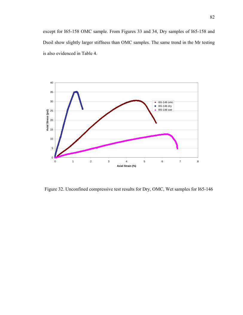
82
except for I65-158 OMC sample. From Figures 33 and 34, Dry samples of I65-158 and
Dsoil show slightly larger stiffness than OMC samples. The same trend in the Mr testing
is also evidenced in Table 4.
0
5
10
15
20
25
30
35
40
0 1 2 3 4 5 6 7 8
Axial Strain (%)
Axi
al S
tres
s (p
si)
I65-146 omcI65-146 dryI65-146 wet
Figure 32. Unconfined compressive test results for Dry, OMC, Wet samples for I65-146
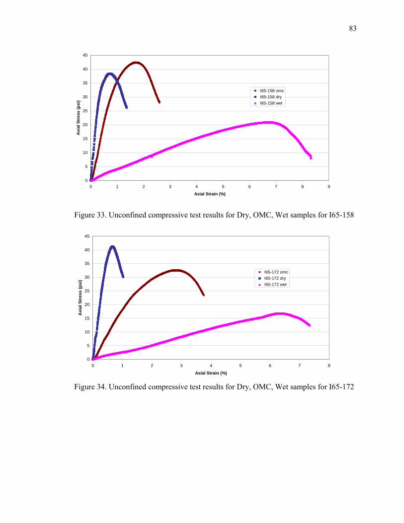
83
0
5
10
15
20
25
30
35
40
45
0 1 2 3 4 5 6 7 8 9
Axial Strain (%)
Axi
al S
tres
s (p
si)
I65-158 omcI65-158 dryI65-158 wet
Figure 33. Unconfined compressive test results for Dry, OMC, Wet samples for I65-158
0
5
10
15
20
25
30
35
40
45
0 1 2 3 4 5 6 7 8
Axial Strain (%)
Axi
al S
tres
s (p
si)
I65-172 omcI65-172 dryI65-172 wet
Figure 34. Unconfined compressive test results for Dry, OMC, Wet samples for I65-172
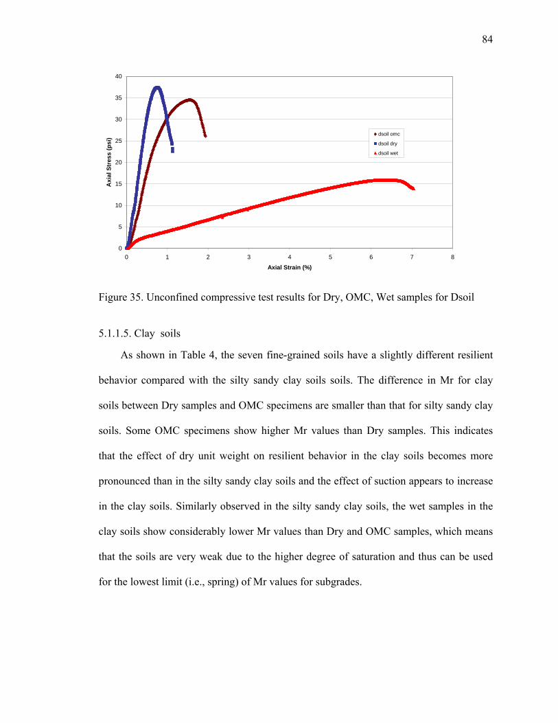
84
0
5
10
15
20
25
30
35
40
0 1 2 3 4 5 6 7 8
Axial Strain (%)
Axi
al S
tres
s (p
si) dsoil omc
dsoil dry
dsoil wet
Figure 35. Unconfined compressive test results for Dry, OMC, Wet samples for Dsoil
5.1.1.5. Clay soils
As shown in Table 4, the seven fine-grained soils have a slightly different resilient
behavior compared with the silty sandy clay soils soils. The difference in Mr for clay
soils between Dry samples and OMC specimens are smaller than that for silty sandy clay
soils. Some OMC specimens show higher Mr values than Dry samples. This indicates
that the effect of dry unit weight on resilient behavior in the clay soils becomes more
pronounced than in the silty sandy clay soils and the effect of suction appears to increase
in the clay soils. Similarly observed in the silty sandy clay soils, the wet samples in the
clay soils show considerably lower Mr values than Dry and OMC samples, which means
that the soils are very weak due to the higher degree of saturation and thus can be used
for the lowest limit (i.e., spring) of Mr values for subgrades.
85
5.1.1.6. Permanent Deformation Behavior
Permanent deformation behavior is not considered in the calculation of Mr values.
This is because the permanent strain is very small for most of the subgrade soils. For
most of the soils tested, the small permanent deformations occurred, especially for Dry
and OMC samples. However, some samples compacted wet of optimum exhibited an
excessive permanent deformation while performing a Mr testing. This caused a
significant difficulty to run a Mr testing up to the final step. Sometimes it was impossible
to run a Mr testing to the end because of the sudden failure of the sample. Most of the
failure was observed to be bulging failure, not shear failure. As can be seen in Figures
32-35, the peak strengths of the wet samples occur at a permanent strain of about seven
percent and the stress ratio of the highest deviator stress (i.e., 10 psi) in Mr testing to the
peak strength are in the range of 50 to 70 percent. This explains why the permanent strain
occurs excessively in the Wet samples. The AASHTO T307 calls for shear test for
samples greater than 5 percent permanent strain. However, it is not practical not to
evaluate Mr values for the soils. The maximum permanent strain was set as 20 percent so
that Mr values can be obtained even for those soils with excessive permanent strain.
Figures 36 and 37 are the results of Mr testing for I65-146 wet sample in the
conditioning stage and in the 5th step, respectively. It was observed in Figure 36 that even
in the conditioning stage the permanent strain occurred to about 10 percent. From Figure
37, the permanent strain approached to about 18 percent and the testing was terminated in
the 5th step. A comparison was made of the resilient modulus between using the original
length and using the deformed length for I65-158 soil, as shown in Figure 38. The
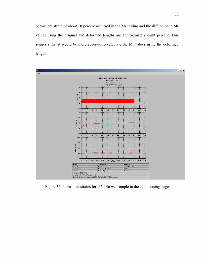
86
permanent strain of about 10 percent occurred in the Mr testing and the difference in Mr
values using the original and deformed lengths are approximately eight percent. This
suggests that it would be more accurate to calculate the Mr values using the deformed
length.
Figure 36. Permanent strains for I65-146 wet sample in the conditioning stage
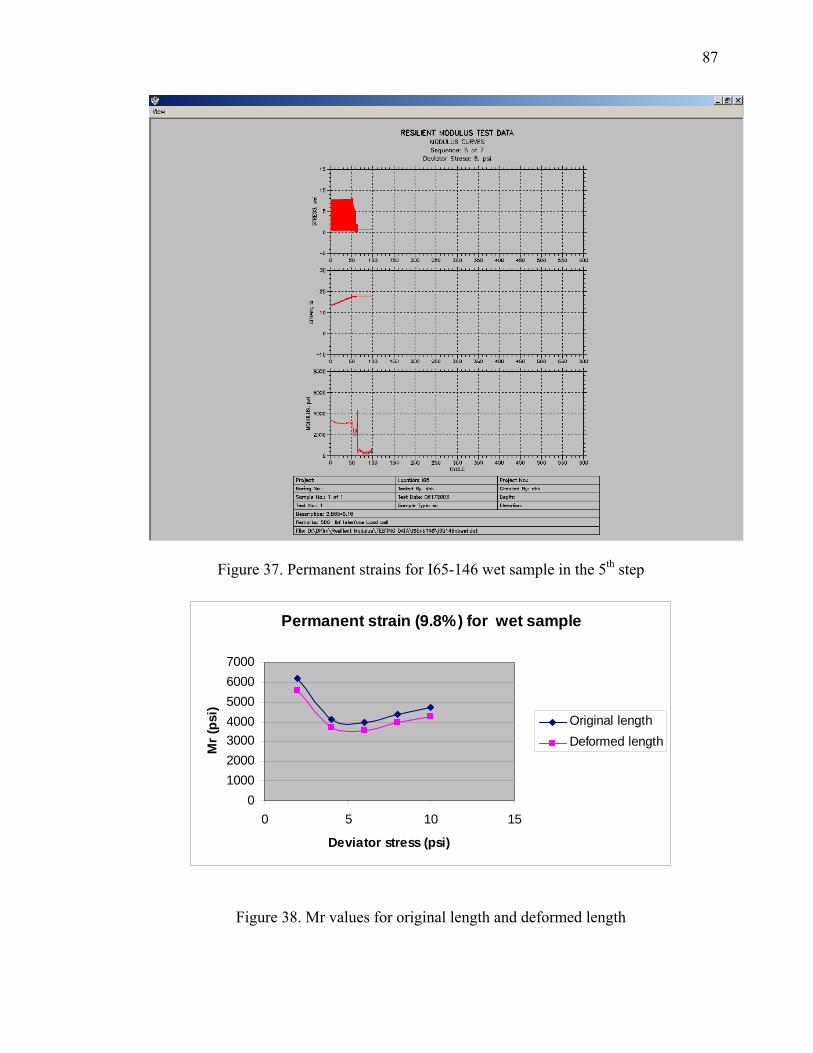
87
Figure 37. Permanent strains for I65-146 wet sample in the 5th step
Permanent strain (9.8%) for wet sample
01000200030004000500060007000
0 5 10 15
Deviator stress (psi)
Mr (
psi)
Original lengthDeformed length
Figure 38. Mr values for original length and deformed length

88
5.1.1.7. Correlation between Unconfined Compressive Test Results and Mr
Some researchers (Lee et al. 1997, Thompson and Robnett 1979) suggested using the
unconfined compressive strength at 1% strain to estimate the resilient modulus, but it was
found that this is not appropriate for our study. Based on the results of unconfined
compressive tests, the three equations were formed primarily using the relationships,
shown in Figure 39:
Mr = k1*f(E)+k2*e(k3*failure strain)+k4*ln(qu)+k5 (5.1)
Where f(E) = aE3 + bE2 + cE + d, k1 = 0.708, k2 = 3171, k3 = -20, k4 = 1284, k5 = -32416,
a = 0.00000008, b = -0.0014, c = 7.711 and d = 2436
Mr = k1*ln(E)+k2*ln(qu)+k3/failure strain+k4 (5.2)
Where k1 = 4720, k2 = -1189, k3 = -23.04 and k4 = -16983
Mr = k1*ln(E)+k2*ln(qu)+k3/failure strain+ k4*ln(Ef)+k5*ln(qf)+k6/yield strain +k7 (5.3)
where k1 = 11267, k2 = 3217, k3 = -76.9, k4 = -8725, k5 = -2587,
k6 = 127.4, k7 = -135134, E = tangent elastic modulus, qu = unconfined compressive
strength, Ef = secant modulus at failure and Mr = resilient modulus at a confining stress
of 2 psi and a deviator stress of 6 psi.
89
As shown in Figure 39, each of the six variables was plotted with respect to resilient
modulus in order to determine the relationships that best correlates to the data. Within the
three types of variables, stresses, strains, and moduli, the relationships were very similar
(e.g. failure stress and peak stress are both best related using a logarithmic equation). In
order to reduce the redundancy of using similar variables, one from each group was
chosen for equations (5.1) and (5.2) after observing the trends on the graph, and choosing
the strongest. Elastic Modulus, peak stress, and failure strain were chosen.
Equation (5.1) uses a third order function of E, the natural logarithm of peak stress,
and an exponential function of failure strain. The function of E and the exponential
function of failure strain each require additional constants to be found in order to relate
them to the resilient modulus. The constants for these functions (a, b, c, d, k3) in the
equation were approximated from the best fit lines shown in Figure 39. The constants in
the final equation (k1, k2, k4, k5) were found using a linear regression analysis. Equation
(5.1) has the highest R2 value, and the lowest standard error. However, the functions are
far more complex and require more constants to be approximated empirically. Also, the
third order polynomial is not preferable, it is possible that this function, despite its good
correlation with the data, would not model other soils as consistently.
Equation (5.2) provides a much simpler relationship between the Mr and the three
variables. By replacing the third order polynomial with a logarithmic function and
replacing the exponential function with an inverse function, the number of required
constants is reduced by five. This also increases the likelihood that the relationship will
accurately model soils, as it is more logical. Statistical analysis shows that this

90
relationship is not as strong as that of equation (5.1), but its simplicity makes it an
attractive alternative.
Equation (5.3) uses all six variables, but uses the relationships used in Equation (5.2)
to relate them to the resilient modulus. It requires seven constants, like Equation (5.2),
but still maintains a more intuitive model for each variable, and the constants are more
simply obtained using a regression. Equation (5.3) has a comparable squared error to
equation (5.1), but has a standard error similar to equation (5.2).
The use of equation (5.2) or (5.3) is recommended. Equation (5.1) is too complex
and too dependent on inconsistent data. Equation (5.2) is simple, and logical, but does not
provide as accurate results as equations (5.1) and (5.3). Equation (5.3) is also logical,
however it is more complicated. It is, however, more accurate than equation (5.2).
FIGURE 3 shows the comparison between predicted and measured Mr values using
equation (5.3), showing that they are in good agreement.
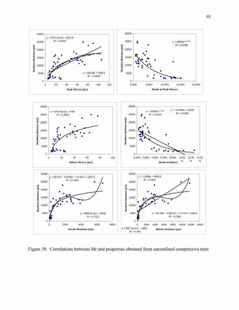
91
y = 5707.2Ln(x) - 8312.9R2 = 0.5202
y = 168.08x + 4348.2R2 = 0.4849
0
5000
10000
15000
20000
25000
30000
0 20 40 60 80 100 120
Peak Stress (psi)
Res
ilien
t Mod
ulus
(psi
)
y = 18905e-15.999x
R2 = 0.6282
0
5000
10000
15000
20000
25000
30000
0.00% 5.00% 10.00% 15.00% 20.00%
Strain at Peak Stress
Res
ilien
t Mod
ulus
(psi
)
y = 5751.9Ln(x) - 6780R2 = 0.4959
0
5000
10000
15000
20000
25000
30000
0 20 40 60 80 100
Failure Stress (psi)
Res
ilien
t Mod
ulus
(psi
)
y = 16425e-21.965x
R2 = 0.6722
y = -147296x + 15420R2 = 0.5259
0
5000
10000
15000
20000
25000
30000
0.00% 2.00% 4.00% 6.00% 8.00% 10.00%
12.00%
14.00%Strain at Failure
Res
ilien
t Mod
ulus
(psi
)
y = 3865.8Ln(x) - 14830R2 = 0.7121
y = 5E-07x3 - 0.0048x2 + 14.467x + 2037.5R2 = 0.7665
0
5000
10000
15000
20000
25000
30000
0 2000 4000 6000 8000
Secant Modulus (psi)
Res
ilien
t Mod
ulus
(psi
)
y = 1.8388x + 5838.8R2 = 0.5967
y = 3627.6Ln(x) - 14851R2 = 0.745
y = 8E-08x3 - 0.0014x2 + 7.7114x + 2435.6R2 = 0.7881
0
5000
10000
15000
20000
25000
30000
0 2000 4000 6000 8000 10000 12000 14000
Elastic Modulus (psi)
Res
ilien
t Mod
ulus
(psi
)
Figure 39. Correlations between Mr and properties obtained from unconfined compressive tests
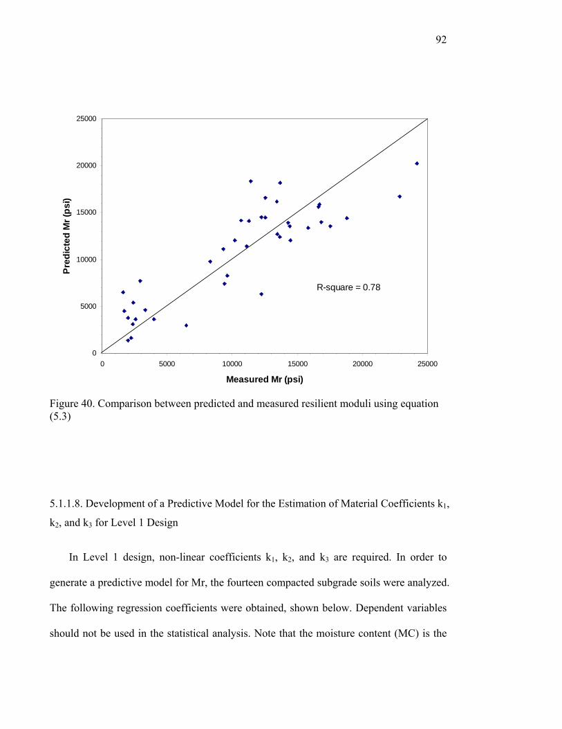
92
0
5000
10000
15000
20000
25000
0 5000 10000 15000 20000 25000
Measured Mr (psi)
Pred
icte
d M
r (ps
i)
R-square = 0.78
Figure 40. Comparison between predicted and measured resilient moduli using equation (5.3)
5.1.1.8. Development of a Predictive Model for the Estimation of Material Coefficients k1,
k2, and k3 for Level 1 Design
In Level 1 design, non-linear coefficients k1, k2, and k3 are required. In order to
generate a predictive model for Mr, the fourteen compacted subgrade soils were analyzed.
The following regression coefficients were obtained, shown below. Dependent variables
should not be used in the statistical analysis. Note that the moisture content (MC) is the
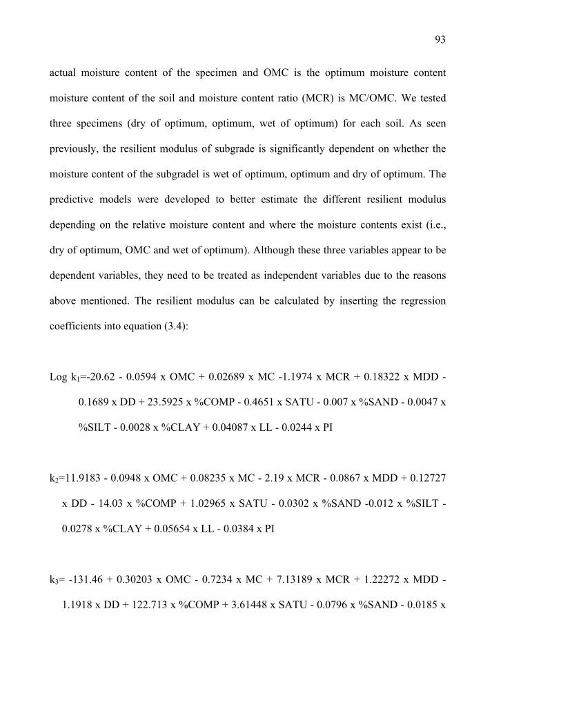
93
actual moisture content of the specimen and OMC is the optimum moisture content
moisture content of the soil and moisture content ratio (MCR) is MC/OMC. We tested
three specimens (dry of optimum, optimum, wet of optimum) for each soil. As seen
previously, the resilient modulus of subgrade is significantly dependent on whether the
moisture content of the subgradel is wet of optimum, optimum and dry of optimum. The
predictive models were developed to better estimate the different resilient modulus
depending on the relative moisture content and where the moisture contents exist (i.e.,
dry of optimum, OMC and wet of optimum). Although these three variables appear to be
dependent variables, they need to be treated as independent variables due to the reasons
above mentioned. The resilient modulus can be calculated by inserting the regression
coefficients into equation (3.4):
Log k1=-20.62 - 0.0594 x OMC + 0.02689 x MC -1.1974 x MCR + 0.18322 x MDD -
0.1689 x DD + 23.5925 x %COMP - 0.4651 x SATU - 0.007 x %SAND - 0.0047 x
%SILT - 0.0028 x %CLAY + 0.04087 x LL - 0.0244 x PI
k2=11.9183 - 0.0948 x OMC + 0.08235 x MC - 2.19 x MCR - 0.0867 x MDD + 0.12727
x DD - 14.03 x %COMP + 1.02965 x SATU - 0.0302 x %SAND -0.012 x %SILT -
0.0278 x %CLAY + 0.05654 x LL - 0.0384 x PI
k3= -131.46 + 0.30203 x OMC - 0.7234 x MC + 7.13189 x MCR + 1.22272 x MDD -
1.1918 x DD + 122.713 x %COMP + 3.61448 x SATU - 0.0796 x %SAND - 0.0185 x
94
%SILT + 0.00251 x %CLAY + 0.03458 x LL + 0.08488 x PI
(5.4)
where OMC (Optimum Moisture Content), MC (Moisture Content), MCR (Moisture
Content Ratio = Moisture Content/ Optimum Moisture Content), DD (Dry Density),
%COMP (Percent Compaction = Dry Density/ Maximum Dry Density), SATU (Degree
of Saturation), %SAND (Percent Sand in Particle Size Distribution Curve), %SILT
(Percent Silt in Particle Size Distribution Curve), %CLAY (Percent Clay in Particle Size
Distribution Curve), LL (Liquid Limit) and PI (Plasticity Index).
Measured and predicted resilient moduli using equation (3.4) are presented in Figure
41. It is shown that the predicted resilient moduli compare well with the measured ones.
y = 1.1365xR2 = 0.8472
0
6000
12000
18000
24000
30000
0 6000 12000 18000 24000 30000
Measured Mr (psi)
Pred
icte
d M
r (ps
i)
95
Figure 41.Comparison between predicted and measured resilient moduli using equation (5.4)
5.1.1.9. Permanent Strain Behavior of Compacted Subgrades
The standard resilient modulus test, AASHTO 307, is designed to model the
behavior of soils under variable loadings similar to those they will experience in the
subgrade. This test limits the number of repetitions to 2000, in order to conserve time and
energy. This is far lower than the amount soil would experience over the design period.
With the low number of repetitions used, this method is not capable of describing
changes in resilient behavior of the soil that may occur due to long term repeated loading,
such as those experienced by subgrades. In order to model the impact of high traffic
volumes on subgrades, a long term resilient modulus test is necessary. For this
experiment, the number of cycles was increased from 2,000 to 20,000. In order to
determine the maximum change in resilient modulus, and to observe the greatest amount
of permanent deformation, the maximum deviator stress (10 psi) and minimum confining
stress (2 psi) used in the standard test were used throughout the entirety of the long term
test. This will result in a conservative estimate, and magnify the potential deterioration of
the soil properties shown in the standard test. Figures 42 and 43 show the changes in
long-term resilient modulus. After about 5,000 repetitions, the resilient modulus shows a
constant value except for the wet Orchard clay, which experienced the excessive
permanent deformation and failed in the initial loading.
Figure 44 shows the long term permanent strain behavior for SR 165 Soil. Compared
to wet soil, soils compacted at OMC and dry of optimum exhibit a negligible amount of
permanent strain. All soils tend to plateau when placed under a consistent stress level,
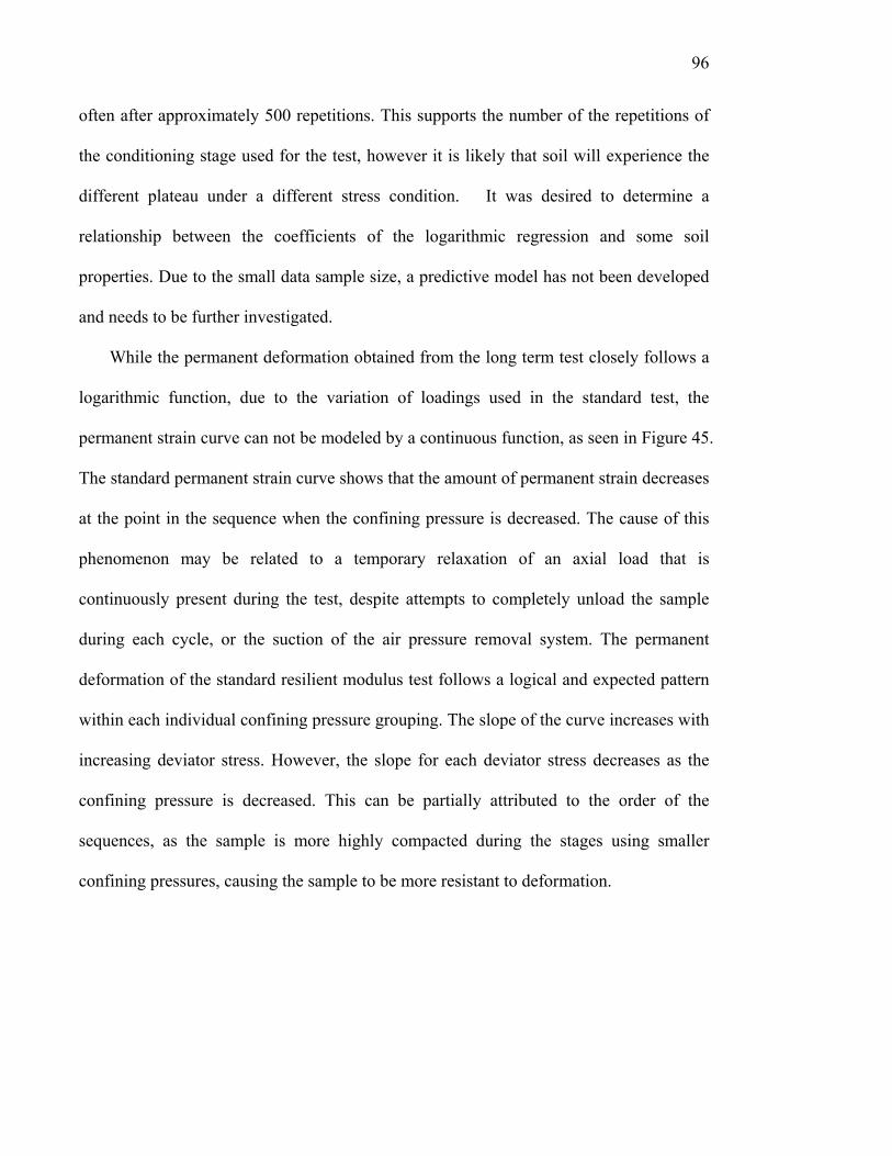
96
often after approximately 500 repetitions. This supports the number of the repetitions of
the conditioning stage used for the test, however it is likely that soil will experience the
different plateau under a different stress condition. It was desired to determine a
relationship between the coefficients of the logarithmic regression and some soil
properties. Due to the small data sample size, a predictive model has not been developed
and needs to be further investigated.
While the permanent deformation obtained from the long term test closely follows a
logarithmic function, due to the variation of loadings used in the standard test, the
permanent strain curve can not be modeled by a continuous function, as seen in Figure 45.
The standard permanent strain curve shows that the amount of permanent strain decreases
at the point in the sequence when the confining pressure is decreased. The cause of this
phenomenon may be related to a temporary relaxation of an axial load that is
continuously present during the test, despite attempts to completely unload the sample
during each cycle, or the suction of the air pressure removal system. The permanent
deformation of the standard resilient modulus test follows a logical and expected pattern
within each individual confining pressure grouping. The slope of the curve increases with
increasing deviator stress. However, the slope for each deviator stress decreases as the
confining pressure is decreased. This can be partially attributed to the order of the
sequences, as the sample is more highly compacted during the stages using smaller
confining pressures, causing the sample to be more resistant to deformation.
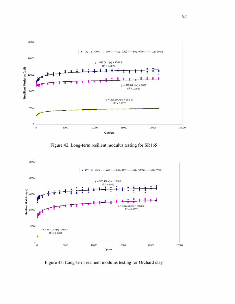
97
y = 552.06Ln(x) + 7764.9R2 = 0.9072
y = 319.63Ln(x) + 7659R2 = 0.7627
y = 316.59Ln(x) + 688.92R2 = 0.9775
0
4000
8000
12000
16000
20000
0 5000 10000 15000 20000 25000
Cycles
Res
ilien
t Mod
ulus
(psi
)
Dry OMC Wet Log. (Dry) Log. (OMC) Log. (Wet)
Figure 42. Long-term resilient modulus testing for SR165
y = 970.19Ln(x) + 13800R2 = 0.8597
y = 1417.5Ln(x) + 3965.5R2 = 0.9557
y = 883.13Ln(x) - 1916.2R2 = 0.9733
0
7000
14000
21000
28000
35000
0 5000 10000 15000 20000 25000
Cycles
Resi
lient
Mod
ulus
(psi
)
Dry OMC Wet Log. (Dry) Log. (OMC) Log. (Wet)
Figure 43. Long-term resilient modulus testing for Orchard clay

98
Figure 44. Permanent Strain of SR 165 Soil (long term Mr test)

99
Figure 45. Permanent strain of SR 165 Soil (standard test)
5.1.2. Results of Resilient Modulus Test on Cohesionless Subgrade Soils
Cohesionless subgrade samples were compacted at optimum moisture contents with
standard Proctor energy. The results of resilient modulus tests for five soils tested are
presented in Figures 46-50. Note that the effect of moisture contents of cohesionless
subgrade soils on resilient modulus is generally negligible due to high permeability of
these soils (Lee et al. 1993). The resilient moduli of cohesionless subgrade soils shown
in Figures 46-50 are slightly higher than those observed in cohesive subgrade soils
although they are poorly graded. As cohesive subgrade soils are more predominant in
Indiana than cohesionless subgrade soils, further investigation has not been conducted.
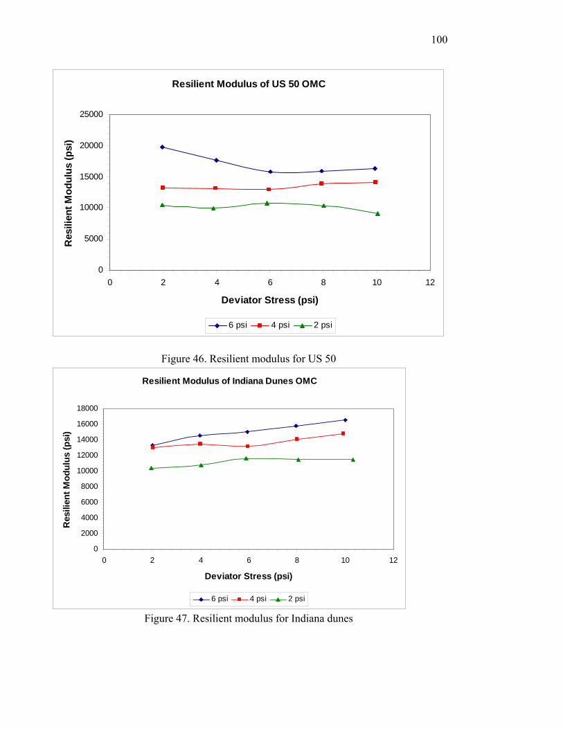
100
Resilient Modulus of US 50 OMC
0
5000
10000
15000
20000
25000
0 2 4 6 8 10 12
Deviator Stress (psi)
Res
ilien
t Mod
ulus
(psi
)
6 psi 4 psi 2 psi
Figure 46. Resilient modulus for US 50
Resilient Modulus of Indiana Dunes OMC
0
2000
4000
6000
8000
10000
12000
14000
16000
18000
0 2 4 6 8 10 12
Deviator Stress (psi)
Res
ilien
t Mod
ulus
(psi
)
6 psi 4 psi 2 psi
Figure 47. Resilient modulus for Indiana dunes

101
Resilient Modulus of N Dune OMC
0
5000
10000
15000
20000
25000
0 2 4 6 8 10 12
Deviator Stress (psi)
Res
ilien
t Mod
ulus
(psi
)
6 psi 4 psi 2 psi
Figure 48. Resilient modulus for N Dune
Resilient Modulus of Wild Cat OMC
0
2000
4000
6000
8000
10000
12000
14000
16000
18000
0 2 4 6 8 10 12
Deviator Stress (psi)
Res
ilien
t Mod
ulus
(psi
)
6 psi 4 psi 2 psi
Figure 49. Resilient modulus for Wild Cat
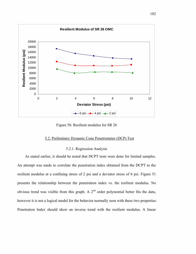
102
Resilient Modulus of SR 26 OMC
0
2000
4000
6000
8000
10000
12000
14000
16000
18000
20000
0 2 4 6 8 10 12
Deviator Stress (psi)
Res
ilien
t Mod
ulus
(psi
)
6 psi 4 psi 2 psi
Figure 50. Resilient modulus for SR 26
5.2. Preliminary Dynamic Cone Penetrometer (DCP) Test
5.2.1. Regression Analysis
As stated earlier, it should be noted that DCPT tests were done for limited samples.
An attempt was made to correlate the penetration index obtained from the DCPT to the
resilient modulus at a confining stress of 2 psi and a deviator stress of 6 psi. Figure 51
presents the relationship between the penetration index vs. the resilient modulus. No
obvious trend was visible from this graph. A 2nd order polynomial better fits the data,
however it is not a logical model for the behavior normally seen with these two properties.
Penetration Index should show an inverse trend with the resilient modulus. A linear
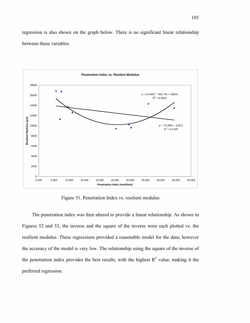
103
regression is also shown on the graph below. There is no significant linear relationship
between these variables.
Penetration Index vs. Resilent Modulus
y = 12.645x2 - 652.79x + 18625R2 = 0.5524
y = -72.285x + 14311R2 = 0.1429
0
2000
4000
6000
8000
10000
12000
14000
16000
18000
0.000 5.000 10.000 15.000 20.000 25.000 30.000 35.000 40.000 45.000 50.000
Penetration Index (mm/blow)
Res
ilien
t Mod
ulus
(psi
)
Figure 51. Penetration Index vs. resilient modulus The penetration index was then altered to provide a linear relationship. As shown in
Figures 52 and 53, the inverse and the square of the inverse were each plotted vs. the
resilient modulus. These regressions provided a reasonable model for the data; however
the accuracy of the model is very low. The relationship using the square of the inverse of
the penetration index provides the best results, with the highest R2 value, making it the
preferred regression.
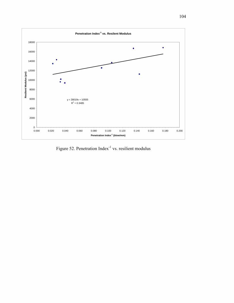
104
Penetration Index-1 vs. Resilent Modulus
y = 28019x + 10555R2 = 0.3485
0
2000
4000
6000
8000
10000
12000
14000
16000
18000
0.000 0.020 0.040 0.060 0.080 0.100 0.120 0.140 0.160 0.180 0.200
Penetration Index-1 (blow/mm)
Res
ilien
t Mod
ulus
(psi
)
Figure 52. Penetration Index-1 vs. resilient modulus

105
Penetration Index-2 vs. ResilentModulus
y = 156754x + 11337R2 = 0.3883
0
2000
4000
6000
8000
10000
12000
14000
16000
18000
0 0.005 0.01 0.015 0.02 0.025 0.03 0.035
Penetration Index-2 (blow2/mm2)
Res
ilien
t Mod
ulus
(psi
)
Figure 53. Penetration Index-2 vs. resilient modulus
Adding soil properties to the model in order to provide a better relationship is
difficult, considering the small amount of available data points. In order to avoid simply
solving a system of equations, additional variables must be kept to a minimum. This has
not yielded a desirable result at this time. In summary, further investigation is needed to
find a relationship between DCPT blow count and the resilient modulus.
106
CHAPTER 6. RESILIENT BEHVAIOR OF LIME AND LKD TREATED
SUBGRADES
6.1. Introduction
This chapter summarizes the resilient modulus tests of soils treated with Lime Kiln
Dust (LKD) that were previously conducted for an INDOT implementation project. This
chapter is mainly based on the paper presented at TRB annual meeting (Kim and Zia
2004).
When a given soil is too weak for a certain specification, one way to improve the
soil so that it satisfies certain engineering properties is to blend it with other natural
materials (Hausmann 1990). Over the past decades, lime treatment has been extensively
used for road construction purposes. Treatment results in increased bearing capacity of
weak subgrades, allowing a reduction in the thickness of the base layer (Bergado et al.
1996, Hausmann 1990). The asphalt or base layer would be thicker if the subgrade had a
very low strength in a pavement structure. The thickness of the asphalt or base layer can
be reduced if the subgrade soil is appropriately treated.
The Indiana Department of Transportation (INDOT) has increased the pace of
improving the current highway network in the past several years. This desire to improve
and expand existing roads is attributed to the importance of mobility for economic
growth, aging of the existing roadway network, etc. (INDOT 2002). To some degree,
chemical-soil modification has become a viable, economic, and minimally disruptive
alternative to in-place modification and/or stabilization. Chemicals such as lime, cement,
107
and flyash are either used to stabilize (increased strength accounted for in pavement
design) or modify (workable to meet compaction) natural soils that are not appropriate
for immediate subgrade construction due to high water contents and low strengths
(INDOT 2002). INDOT has recently made considerable efforts to achieve effective road-
bed improvement and revised subgrade specifications recently to allow contactors to
choose appropriate subgrade construction methods based on soil types, economy, traffic
limitations, and environmental considerations.
In subgrade improvement using lime, quicklime (CaO) or hydrated lime(Ca(OH)2) is
generally used to facilitate subgrade construction in INDOT. Treated soils with lime
exhibit improved plasticity, workability, and volume change characteristics. Quicklime
(calcium oxide) is formed as a coarse-grained powder. Lime is primarily used for the
treatment of fine grained soils (i.e. such as A-4, A-6 and A-7 following the AASHTO
classfication), especially clayey soils. The short-term reactions of the soil-lime mixture in
the presence of water result in hydration and flocculation (ion exchange) due to the clay
minerals. In a favorable environment such as temperature, the lime is a source of free
calcium. The long-term reactions are related to cementation. Quicklime reacts with water
very quickly in the soil. This drying action is particularly beneficial in the treatment of
moist clays. When lime is mixed with clay, sodium and other cations absorbed to the clay
mineral surfaces are exchanged with calcium. This cation exchange affects the way the
structural components of the clay minerals are linked together. Lime causes clay to
coagulate, aggregate, or flocculate. The plasticity of clay is reduced, making it more
workable and potentially increasing its stiffness and strength. Cementation is the main
contributor to the strength of the stabilized soil. The higher the surface area of the soil,
108
the more effective is this process. Note that lime is not suitable for improving clean sands
or gravels. Practical lime admixtures range from 2 to 8 %. Thus, lime has some
advantages in clay subgrade stabilization, which increases strength of clay soils , and
reduces shrinkage and swelling.
Although LKD has recently been permitted to be used in soil modification by
INDOT, unlike lime, it has not been approved for subgrade stabilization due to limited
experience with it. Also, the increased strength of LKD treated soils is not considered in
design and the material parameters of the original natural soils are applied in design
practice for a conservative design. Therefore, the objective of this study was to evaluate
the mechanical benefits of the LKD for use in soil modification and stabilization under
similar environmental conditions.
6.2. Engineering Properties of Soils Treated with LKD and LIME
LKD (Lime Kiln Dust) is a by-product collected in dust collection systems from the
manufacture of lime. LKD is mainly composed of calcium oxide, but contains varying
amounts of calcium sulphate (depending on the sulfur level of the fuel), fly ash, and
limestone (Francis 2003). Lime is manufactured from limestone (CaCO3) by heating it to
a high temperature (about 2000o F) to separate and drive off the carbon dioxide (CO2).
Although extensive research on lime and Cement Kiln Dust (CKD) has been done,
mechanical evaluation studies on LKD are quite limited (Parson 1995, Ciesielski and
Collins 1995, Henkel 1997, Daita et al. 2005). Due to the limited data available for
LKD, it would be helpful to study the characteristics of lime-treated soils. The behavior
of lime treated soils is primarily dependent on soil types, lime contents, temperature,
curing time (TRB 1987).
109
Moisture-density relationships of lime treated soils change constantly. Maximum
dry density and Optimum Moisture Content (OMC) are two important parameters used to
characterize compaction. Maximum dry density decreases as optimum moisture
increases when a lime-soil mixture is allowed to cure (TRB 1987, Daita et al. 2005). It is
important to realize that this density reduction is not due to poor compaction but rather to
the fact that the material is changing. Based on the study done by Heckel (1997), LKD
also reduces the maximum dry density and increases the OMC, which is similarly
observed in lime-soil mixtures.
Improvement of the uncured unconfined compression strength, CBR, plasticity of
the soil-lime mixture was observed by many studies (Thompson 1966, Thompson 1969,
Neubauer and Thompson 1972). This immediate improvement helps expedite
construction when soft, highly plastic, cohesive soils create mobility problems for
wheeled equipments (TRB 1987). According to Heckel (1987), it is also noted that LKD
creates an increase in unconfined strength. One important factor of the lime-treated soils
is hardening resulting from curing with time. It should be noted that considerable
improvement of strength continues over 10 years in some cases (TRB 1987). Soil-lime
mixtures lead to substantial increases in cohesion resulting from cementation, but not in
the internal angle of friction.
6.2. Experimental Program
6.2.1. LKD and Hydrated Lime used in the study
According to INDOT specification, hydrated lime or quick lime and LKD can be
used in the range of 4±0.5 % and 5±1 % by weight of soil for modification, respectively.
110
For subgrade modification, a pH test is generally performed to determine the amount of
lime or LKD. In our study, 5 % LKD and 5 % hydrated lime contents were used. The
LKD contained 60 % of calcium and magnesium oxides and the hydrated lime contained
90 % of calcium and magnesium hydroxides/ oxides.
6.2.2. Soils used in the study
Five typical fine-grained soils in Indiana which are appropriate for lime treatment
were collected from I-94, US-41, SR-37, and SR-46. For distinction, each soil is
designated as, for example, A-4 (US-41) indicating an A-4 soil collected from US-41.
Figure 54 shows the grain size distribution and Table 5 represents the index test results
for soils used in the experimental program. The soils are classified as A-4, A-6, and A-7-
6 under the AASHTO classification; ML, CL and CH under the USCS classification; and
as Si, Si-LO, CL-LO, and CL under INDOT textural Soil Classification (Figure 55).
Gradation and Atterberg limits tests were performed following AASHTO T-89 and
AASHTO T-90. Standard Proctor tests were performed according to AASHTO T-99.
Figure 56 shows the compaction curves for determining maximum dry density and
optimum moisture content. As seen in Figure 56, the maximum dry density and optimum
moisture content are in the range of 98 – 115 pcf (15.4 – 18 kN/m3) and 12 – 23 %,
respectively. In our study, three samples of each soil (i.e. untreated, 5 % lime treated and
5 % Lime Kiln Dust (LKD)) were prepared. In addition, untreated and treated soils were
prepared with 90 %, 95 % (compacted at dry of optimum) and 100 % compaction to
assess the unconfined compression strength, CBR, swell potential and resilient modulus.
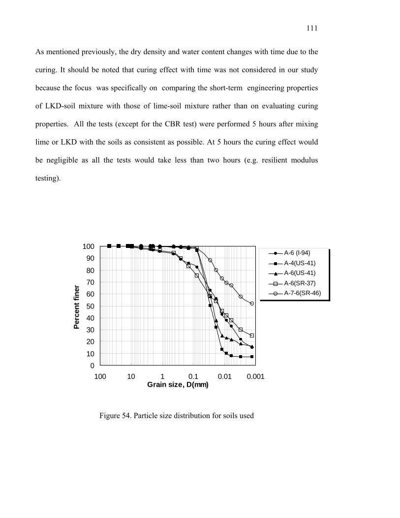
111
As mentioned previously, the dry density and water content changes with time due to the
curing. It should be noted that curing effect with time was not considered in our study
because the focus was specifically on comparing the short-term engineering properties
of LKD-soil mixture with those of lime-soil mixture rather than on evaluating curing
properties. All the tests (except for the CBR test) were performed 5 hours after mixing
lime or LKD with the soils as consistent as possible. At 5 hours the curing effect would
be negligible as all the tests would take less than two hours (e.g. resilient modulus
testing).
010
20304050
607080
90100
0.0010.010.1110100Grain size, D(mm)
Perc
ent f
iner
A-6 (I-94)A-4(US-41)A-6(US-41)A-6(SR-37)A-7-6(SR-46)
Figure 54. Particle size distribution for soils used
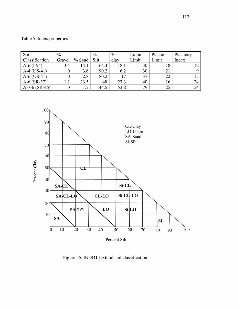
112
Table 5. Index properties
Soil Classification
% Gravel % Sand
% Silt
% clay
Liquid Limit
Plastic Limit
Plasticity Index
A-6 (I-94) 3.4 14.1 64.4 18.1 30 18 12A-4 (US-41) 0 3.6 90.2 6.2 30 21 9A-6 (US-41) 0 2.8 80.2 17 37 22 15A-6 (SR-37) 1.2 23.5 48 27.3 40 16 24A-7-6 (SR-46) 0 1.7 44.5 53.8 79 25 54
Figure 55. INDOT textural soil classification
Si-CL-LO
Si-CL
CL-LOSA-CL-LO
SA Si-LOSA-LO
CL
SA-CL
Si
LO
CL-Clay LO-Loam SA-Sand Si-Silt
Percent Silt
10 20 30 40 50
10
60 100 0 80 90 70
20
30
40
50
60
70
80
90
100
Perc
ent C
lay
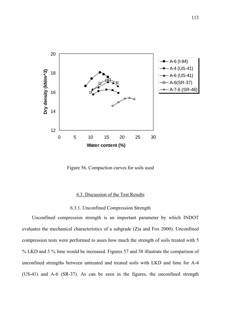
113
12
14
16
18
20
0 5 10 15 20 25 30
Water content (%)
Dry
den
sity
(kN
/m^3
)
A-6 (I-94)A-4 (US-41)A-6 (US-41)A-6(SR-37)A-7-6 (SR-46)
Figure 56. Compaction curves for soils used
6.3. Discussion of the Test Results
6.3.1. Unconfined Compression Strength
Unconfined compression strength is an important parameter by which INDOT
evaluates the mechanical characteristics of a subgrade (Zia and Fox 2000). Unconfined
compression tests were performed to asses how much the strength of soils treated with 5
% LKD and 5 % lime would be increased. Figures 57 and 58 illustrate the comparison of
unconfined strengths between untreated and treated soils with LKD and lime for A-4
(US-41) and A-6 (SR-37). As can be seen in the figures, the unconfined strength
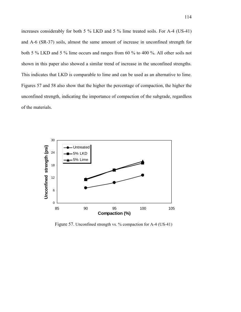
114
increases considerably for both 5 % LKD and 5 % lime treated soils. For A-4 (US-41)
and A-6 (SR-37) soils, almost the same amount of increase in unconfined strength for
both 5 % LKD and 5 % lime occurs and ranges from 60 % to 400 %. All other soils not
shown in this paper also showed a similar trend of increase in the unconfined strengths.
This indicates that LKD is comparable to lime and can be used as an alternative to lime.
Figures 57 and 58 also show that the higher the percentage of compaction, the higher the
unconfined strength, indicating the importance of compaction of the subgrade, regardless
of the materials.
0
6
12
18
24
30
85 90 95 100 105Compaction (%)
Unc
onfin
ed s
tren
gth
(psi
) Untreated5% LKD5% Lime
Figure 57. Unconfined strength vs. % compaction for A-4 (US-41)

115
0
30
60
90
120
85 90 95 100 105Compaction (%)
Unc
onfin
ed s
tren
gth
(psi
) Untreated5% LKD5% Lime
Figure 58. Unconfined strength vs. % compaction for A-6 (SR-37)
6.3.2. CBR and Swell Potential
Although it has already been recommended to use the resilient modulus value for
characterizing subgrade materials, CBR values are still used in design practice due to the
limited availability of resilient modulus values for soils. Table 6 presents CBR values and
the amount of swell measured after 4 days of soaking for untreated and untreated soils
compacted at optimum moisture content. As seen in Table 6, the maximum dry densities
become smaller and optimum moisture contents become larger for treated soils than those
for untreated soils. It is noted that much larger CBR values are achieved for both 5 %
lime and 5 % LKD soil mixtures than those for untreated soils. Except for A-7-6 (SR-37),
the largest CBR values are were achieved for 5 % LKD treated soils. CBR values for
treated soils were in the range of 25 to 70 while those for untreated soils ranged from 3 to
18. It should be noted that the swell potential would vary for different percent

116
compactions; the smaller the water contents, the higher the swell potential due to a
greater portion of air trapped in the soil. For this reason, a larger amount of swell was
observed at 90 % and 95 % compaction compared with 100% compaction. It is apparent
that blending with 5 % lime and 5 % LKD causes the swell potential to decrease
remarkably. As can be seen in the table, a higher reduction in swell potential was
observed more often in the 5 % lime treated soils than that in the 5 % LKD treated soils.
LKD treated soils, however, also showed substantial improvement in swell potential,
compared with untreated soils. This implies that soils having high clay contents can
decrease in the swell potential when mixed with 5 % LKD. For A-4 (US-41) soil,
interestingly the swell potential of LKD treated soil increased slightly. This appears to be
due to the negligible swell potential of the untreated soil as it has a fairly high silt content
as shown in Table 5.

117
Table 6. CBR and swell potential for untreated and 5 % LKD and 5 % lime treated soils compacted at OMC
Condition Maximum Molded Molded Percent Swell CBR
Soil density OMC density water content
maximum density day 4
(kN/m3) (%) (kN/m3) (%) (%) A-6 (I-94) Untreated 18.1 13 18.0 13.5 99.5 0.22 3.1 5 % LIME 17.3 17 17.1 17 98.8 0.17 45.3 5 % LKD 17.3 17 17.6 16 102.1 0.19 68.7A-4 (US-41) Untreated 16.3 15 16.4 14.8 100.3 0.07 17.3 5 % LIME 16.3 17 16.5 16.9 101.3 0.04 32.3 5 % LKD 16.2 17 16.2 17.5 100.1 0.26 52.4A-6 (US-41) Untreated 17.1 16 17.1 16.8 99.9 0.33 11.3 5 % LIME 16.5 19 16.0 19.5 97.2 0.04 39.1 5 % LKD 16.3 18 16.8 18.6 102.6 0.22 64.5A-6 (SR-37) Untreated 17.3 16 17.4 16.1 100.6 1.77 5.9 5 % LIME 17.7 18 17.4 18.2 98.1 0.17 63.1 5 % LKD 17.4 13 17.4 12.5 99.9 0.68 68A-7-6 (SR-46) Untreated 15.4 23 15.6 23 101.5 3.53 2.8 5 % LIME 15.2 27 14.8 27.6 97.1 0.79 44 5 % LKD 15.1 25 14.8 26 98.0 1.72 25.3
6.3.3. Resilient Behavior of Soil-LKD and Soil-Lime Mixtures
Since the AASHTO design guide in 1986 recommended highway agencies use
resilient modulus (Mr) in the design of pavements, resilient modulus has been used to
characterize subgrade. Resilient modulus testing was performed according to the stress
sequence of AASHTO T-307. In Mr testing, confining stresses of 2, 4, and 6 psi were
applied and deviator stresses of 2, 4, 6, 8 and 10 psi were used for each confining stress.
Specimens for Mr testing were prepared and wrapped with a vinyl bag for 5 hours like the
other tests to maintain the mixing water content before testing. Generally, the resilient
behaviors of fine- grained soils are primarily dependent on the confining pressure; the
higher the confining stress, the higher the resilient modulus (Lee et al. 1997, Thompson
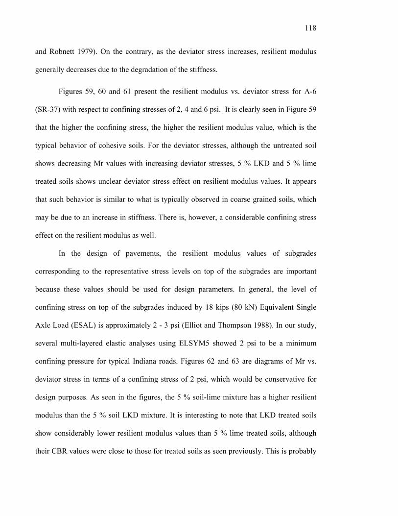
118
and Robnett 1979). On the contrary, as the deviator stress increases, resilient modulus
generally decreases due to the degradation of the stiffness.
Figures 59, 60 and 61 present the resilient modulus vs. deviator stress for A-6
(SR-37) with respect to confining stresses of 2, 4 and 6 psi. It is clearly seen in Figure 59
that the higher the confining stress, the higher the resilient modulus value, which is the
typical behavior of cohesive soils. For the deviator stresses, although the untreated soil
shows decreasing Mr values with increasing deviator stresses, 5 % LKD and 5 % lime
treated soils shows unclear deviator stress effect on resilient modulus values. It appears
that such behavior is similar to what is typically observed in coarse grained soils, which
may be due to an increase in stiffness. There is, however, a considerable confining stress
effect on the resilient modulus as well.
In the design of pavements, the resilient modulus values of subgrades
corresponding to the representative stress levels on top of the subgrades are important
because these values should be used for design parameters. In general, the level of
confining stress on top of the subgrades induced by 18 kips (80 kN) Equivalent Single
Axle Load (ESAL) is approximately 2 - 3 psi (Elliot and Thompson 1988). In our study,
several multi-layered elastic analyses using ELSYM5 showed 2 psi to be a minimum
confining pressure for typical Indiana roads. Figures 62 and 63 are diagrams of Mr vs.
deviator stress in terms of a confining stress of 2 psi, which would be conservative for
design purposes. As seen in the figures, the 5 % soil-lime mixture has a higher resilient
modulus than the 5 % soil LKD mixture. It is interesting to note that LKD treated soils
show considerably lower resilient modulus values than 5 % lime treated soils, although
their CBR values were close to those for treated soils as seen previously. This is probably
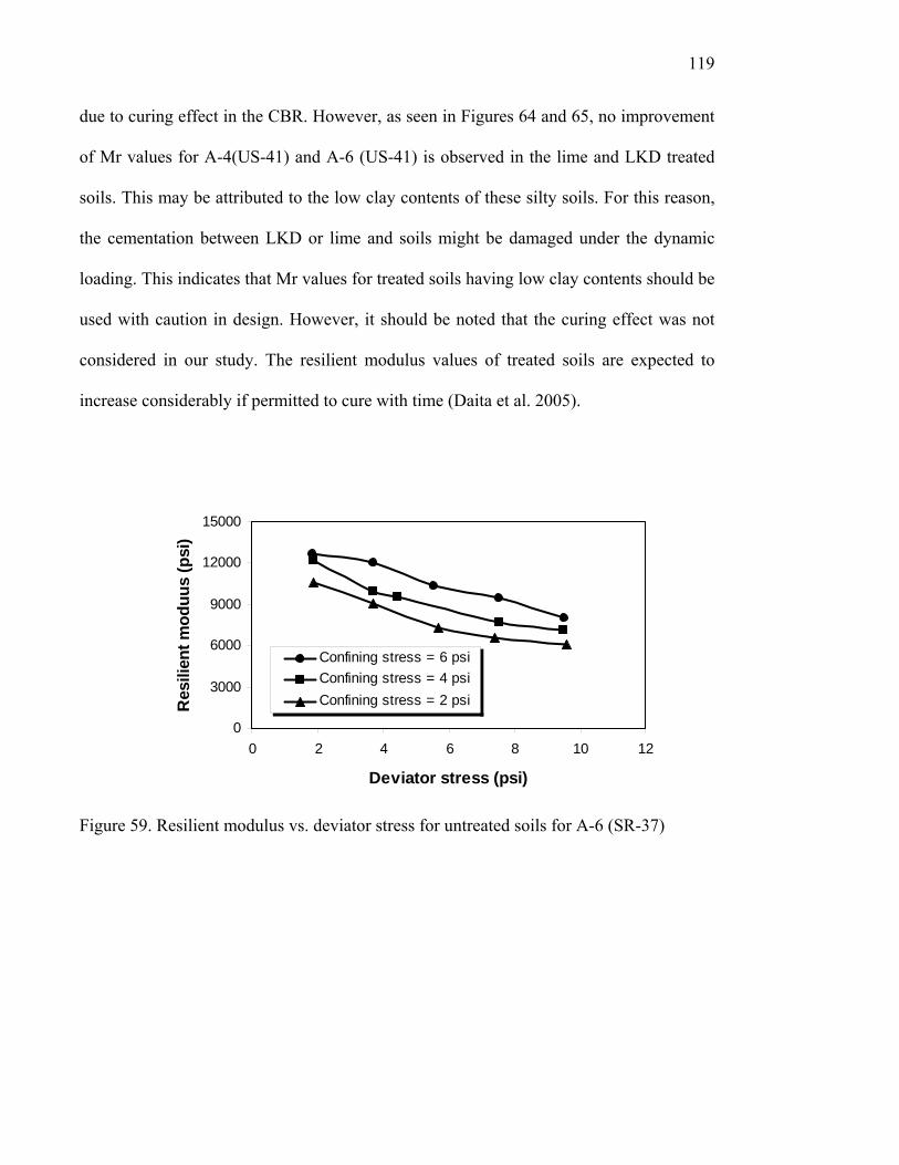
119
due to curing effect in the CBR. However, as seen in Figures 64 and 65, no improvement
of Mr values for A-4(US-41) and A-6 (US-41) is observed in the lime and LKD treated
soils. This may be attributed to the low clay contents of these silty soils. For this reason,
the cementation between LKD or lime and soils might be damaged under the dynamic
loading. This indicates that Mr values for treated soils having low clay contents should be
used with caution in design. However, it should be noted that the curing effect was not
considered in our study. The resilient modulus values of treated soils are expected to
increase considerably if permitted to cure with time (Daita et al. 2005).
0
3000
6000
9000
12000
15000
0 2 4 6 8 10 12
Deviator stress (psi)
Res
ilien
t mod
uus
(psi
)
Confining stress = 6 psiConfining stress = 4 psiConfining stress = 2 psi
Figure 59. Resilient modulus vs. deviator stress for untreated soils for A-6 (SR-37)
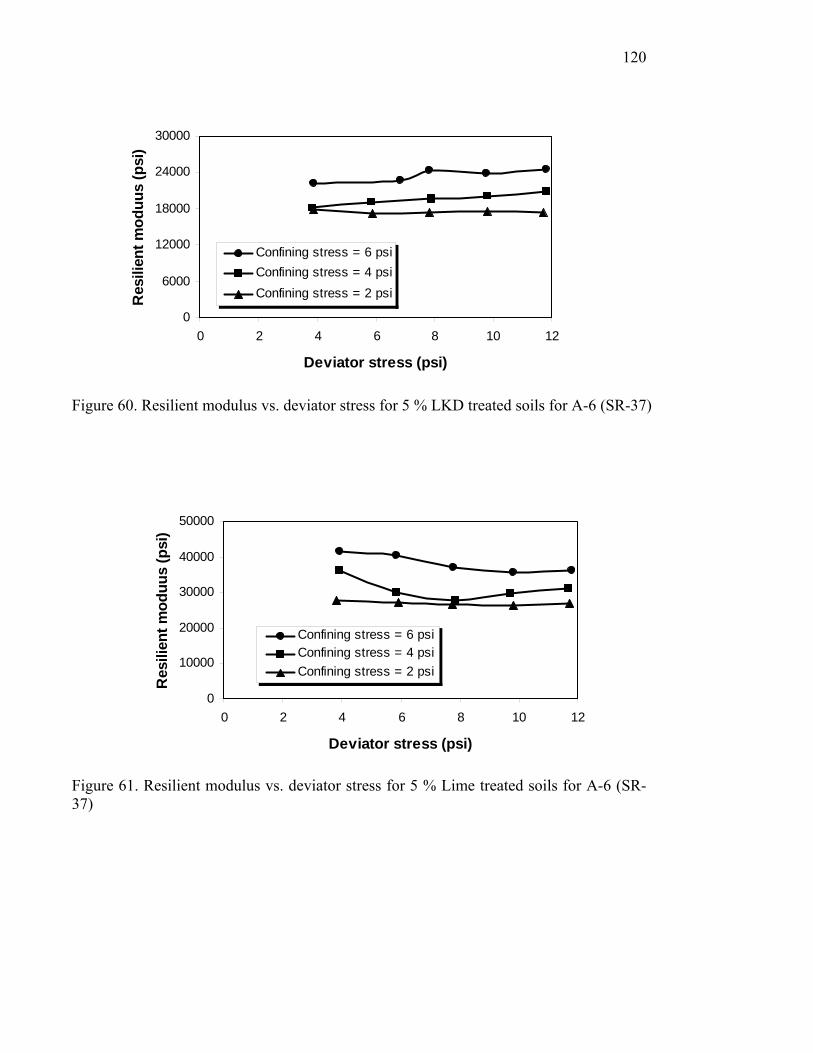
120
0
6000
12000
18000
24000
30000
0 2 4 6 8 10 12
Deviator stress (psi)
Res
ilien
t mod
uus
(psi
)
Confining stress = 6 psiConfining stress = 4 psiConfining stress = 2 psi
Figure 60. Resilient modulus vs. deviator stress for 5 % LKD treated soils for A-6 (SR-37)
0
10000
20000
30000
40000
50000
0 2 4 6 8 10 12
Deviator stress (psi)
Res
ilien
t mod
uus
(psi
)
Confining stress = 6 psiConfining stress = 4 psiConfining stress = 2 psi
Figure 61. Resilient modulus vs. deviator stress for 5 % Lime treated soils for A-6 (SR-37)
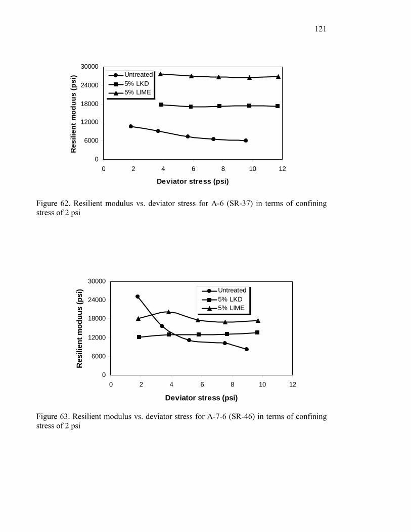
121
0
6000
12000
18000
24000
30000
0 2 4 6 8 10 12
Deviator stress (psi)
Res
ilien
t mod
uus
(psi
) Untreated5% LKD5% LIME
Figure 62. Resilient modulus vs. deviator stress for A-6 (SR-37) in terms of confining stress of 2 psi
0
6000
12000
18000
24000
30000
0 2 4 6 8 10 12
Deviator stress (psi)
Res
ilien
t mod
uus
(psi
) Untreated5% LKD5% LIME
Figure 63. Resilient modulus vs. deviator stress for A-7-6 (SR-46) in terms of confining stress of 2 psi
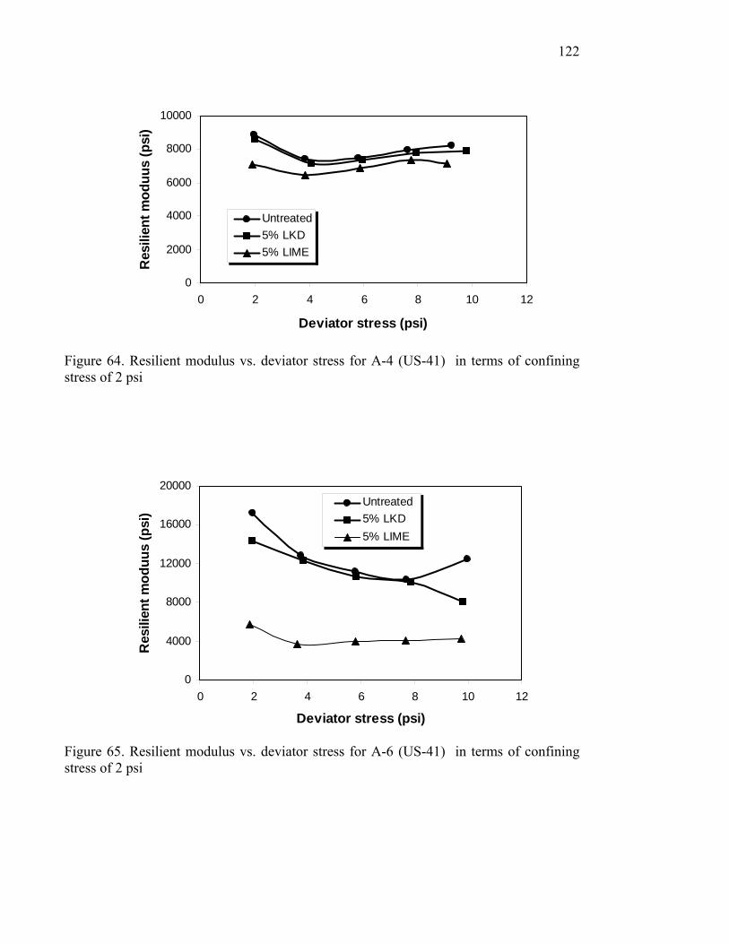
122
0
2000
4000
6000
8000
10000
0 2 4 6 8 10 12
Deviator stress (psi)
Res
ilien
t mod
uus
(psi
)
Untreated5% LKD5% LIME
Figure 64. Resilient modulus vs. deviator stress for A-4 (US-41) in terms of confining stress of 2 psi
0
4000
8000
12000
16000
20000
0 2 4 6 8 10 12
Deviator stress (psi)
Res
ilien
t mod
uus
(psi
)
Untreated5% LKD5% LIME
Figure 65. Resilient modulus vs. deviator stress for A-6 (US-41) in terms of confining stress of 2 psi
123
Generally, resilient behavior of subgrade soils can be described by the Uzan model
(Uzan 1985), also known as the universal model, taking into account confining and
deviator stresses (Santa 1994). The predicted Mr values were obtained from the
following equation:
32 )()(1k
a
dk
aa pp
pkMr σθ= (6.1)
where, k1, k2, k3, = regression coefficients; θ = sum of principal stresses; pa = reference
pressure = 100 kpa ≈ 1 kgf/cm2 ≈ 2000 psf ≈ 14.5 psi; and σd = deviator stress in the
same unit as pa.
It is noted that use of equation (6.1) for different soils cannot produce satisfactory
correlation. In order to develop predictive models that account for the soil properties
based on the all the Mr testing data for five untreated and treated soils, three equations,
shown in Table 7 (shown only for untreated soils), to estimate the regression coefficient
k1, k2, and k3 were developed through multiple regression analyses in terms of 12 soil
variables which can be easily obtained in the Sieve Analysis, Atterberg’s Limit test, and
Standard Proctor compaction test. The variables are the following: OMC, MC (moisture
content), MCR (Moisture Content Ratio = Moisture content/ Optimum Moisture Content),
MDD (Maximum dry density), DD (dry density), SATU (Degree of saturation),
%Compaction, %sand (percent sand in Particle size distribution curve), %Silt (percent
sand in Particle size distribution curve), %CLAY (percent sand in Particle size
distribution curve), LL (Liquid Limit) and PI (Plastic Index).
Figures 66, 67 and 68 show a plot of measured Mr vs. predicted Mr for the five
LKD and five lime treated soils tested in this study. The predicted and measured Mr
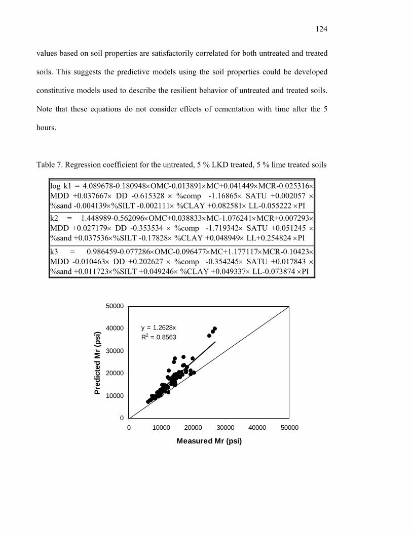
124
values based on soil properties are satisfactorily correlated for both untreated and treated
soils. This suggests the predictive models using the soil properties could be developed
constitutive models used to describe the resilient behavior of untreated and treated soils.
Note that these equations do not consider effects of cementation with time after the 5
hours.
Table 7. Regression coefficient for the untreated, 5 % LKD treated, 5 % lime treated soils
log k1 = 4.089678-0.180948×OMC-0.013891×MC+0.041449×MCR-0.025316× MDD +0.037667× DD -0.615328 × %comp -1.16865× SATU +0.002057 × %sand -0.004139×%SILT -0.002111× %CLAY +0.082581× LL-0.055222 ×PI k2 = 1.448989-0.562096×OMC+0.038833×MC-1.076241×MCR+0.007293× MDD +0.027179× DD -0.353534 × %comp -1.719342× SATU +0.051245 × %sand +0.037536×%SILT -0.17828× %CLAY +0.048949× LL+0.254824 ×PI
k3 = 0.986459-0.077286×OMC-0.096477×MC+1.177117×MCR-0.10423× MDD -0.010463× DD +0.202627 × %comp -0.354245× SATU +0.017843 × %sand +0.011723×%SILT +0.049246× %CLAY +0.049337× LL-0.073874 ×PI
y = 1.2628xR2 = 0.8563
0
10000
20000
30000
40000
50000
0 10000 20000 30000 40000 50000
Measured Mr (psi)
Pred
icte
d M
r (ps
i)

125
Figure 66. Measured vs. predicted Mr for untreated soils
y = 0.9939xR2 = 0.9363
0
10000
20000
30000
40000
0 10000 20000 30000 40000
Measured Mr (psi)
Pred
icte
d M
r (ps
i)
Figure 67. Measured vs. predicted Mr for 5 % LKD treated soils
y = 0.997xR2 = 0.9896
0
10000
20000
30000
40000
0 10000 20000 30000 40000
Measured Mr (psi)
Pred
icte
d M
r (ps
i)
Figure 68. Measured vs. predicted Mr for 5 % Lime treated soils
126
6.4. Summary
Laboratory evaluation was done to identify possible benefits of Lime Kiln Dust for
subgrade modification and stabilization. 5 % LKD and 5 % hydrated lime were added to
typical fine-grained soils encountered in Indiana. Unconfined strength, CBR and resilient
modulus tests were performed on untreated, 5 % LKD treated, and 5 % lime treated
samples with 90%, 95 % and 100% compactions. As a result of the laboratory tests, the
following conclusions can be drawn. It is noted that conclusions based on five hours of
curing may differ from conclusions that can be made after 7 day, 14 day. or during the
life of the pavement.
• Mixtures of fine grained soils with 5 % lime or 5 % LKD substantially improve
unconfined strength up to 60 % - 400 %. For both untreated and treated soils, as the
percentage of compaction increases, the unconfined compression strength increases. This
suggests the importance of compaction of the subgrade, regardless of the materials.
• CBR values are remarkably improved with LKD and lime treatment and swell potential
is generally reduced. Larger CBR values are achieved by 5 % LKD treatment than by 5
% lime treatment. Therefore, use of LKD for subgrade improvement is as promising as
lime.
127
• Resilient behavior of LKD and lime treated soils shows a similar tendency to fine-
grained soils in terms of confining stresses. However, unlike untreated soils, the effect of
deviator stress on the resilient modulus is negligible for treated soils. This would be
attributed to the increased stiffness in the treated soils compared with the untreated soils.
• Although the CBR values for soils treated with LKD and lime were higher, resilient
modulus values for treated soils for A-4 (US-41) and A-6 (US-41) were lower than those
for untreated soils. It appears that this may be due to the low clay contents of these silty
soils, or to the presence of cementation in the CBR test by soaking of the specimens, and
to the different mechanisms of the CBR test (static test) and resilient modulus test
(dynamic repeated test). Therefore, soils with high clay contents are advisable when
mixed with LKD or lime, as evidenced by A-6 (SR-37) and A-7-6(SR-46). More resilient
modulus testing for LKD and lime treated soils needs to be done to draw a complete
conclusion on the resilient modulus behavior of these treated soils in conjunction with
more CBR tests.
• Regression equations were developed for untreated, 5 % LKD and 5 % lime treated
soils following the Uzan model considering the soil physical parameters to estimate Mr
values. Predicted Mr values are well correlated with measured Mr values for 5 hours of
curing.
In Indiana, LKD has been used for subgrade modification, but not for stabilization
due to the limited available data for implementation. The improved properties such as
unconfined, CBR, resilient modulus values achieved by the modification have not been
taken into account in design. Results of the unconfined strength, CBR, resilient modulus

128
tests for untreated, 5 % LKD and 5 % lime treated soils suggest that LKD could be
effectively used as an alternative to lime. This leads to the beneficial impact on the use of
LKD for both subgrade modification and stabilization. Further study on the resilient
behavior is recommended to accumulate typical resilient modulus values for different
types of soils with LKD and Lime treatment for more realistic design.
129
CHAPTER 7. THEORETICAL INVESTIGATION OF BEHAVIOR OF
SUBGRADES
7.1. Mathematical Expression of the Loading Cycles in AASHTO T307 The basic principle of the loading adopted in AASHTO T 307 is the simulation of a
typical moving load in a sinusoidal form. The peak point of the loading is analogous to
the loading condition where the traffic is immediately above the subgrade. A soil sample
subjected to resilient modulus testing can be simply modeled as a one-dimensional forced
vibration of a spring-mass system, as shown in equation (7.1).
)(''' tFkYcYmY =++ (7.1)
Where m = W/g, W = weight (Unit: kN), g = gravity acceleration, c = damping ratio
(non-dimensional), Y = vertical displacement and F(t) = the applied load. For simplicity,
mass of top cap and ram in equation (7.1) is neglected.
Fourier series can be used to represent a given periodic function F(t) in terms of
cosine and sine functions. If a function F(t) of period p=2L has a Fourier series, we can
express this series as follows:
∑∞
=⎟⎠⎞
⎜⎝⎛ ++=
10 )sin()cos(()(
nnn t
Lnbt
LnaatF ππ (7.2)
130
∫−
=L
L
dttfL
a )(21
0 (7.3)
dtL
tndttfL
aL
Ln
πcos)(21∫−
= n = 1, 2…., (7.4)
dtL
tndttfL
bL
Ln
πsin)(21∫−
= n = 1, 2…., (7.5)
An example of the schematic load pulse for a deviator stress of 2 psi in AASHTO
307 is shown in Figure 69. As can be seen in Figure 69, for 0.1 second the deviator stress
is applied and for 0.9 second, no load is applied, and then this is repeated for a certain
level of stress. The load pulse shown in Figure 69 can be expressed as:
)2
)20cos(1()( maxttf πσ −
= 0‹t‹0.1s (7.6)
0)( =tf 0.1s‹t‹1s (7.7)
As p = 2L=1 second, L=1/2 second (7.8)
Substituting equations (7.6), (7.7) and (7.8) into equation (7.2) allows F(t) to be
obtained. The plot of F(t) is shown in Figure 70. After substituting the obtained F(t) into
equation (7.1) and solving the 2nd order differential equation (7.1), (assuming c = 0.2) ,
one can obtain the vertical displacement of a soil sample as a function of the weight of
sample and the spring constant as given by:
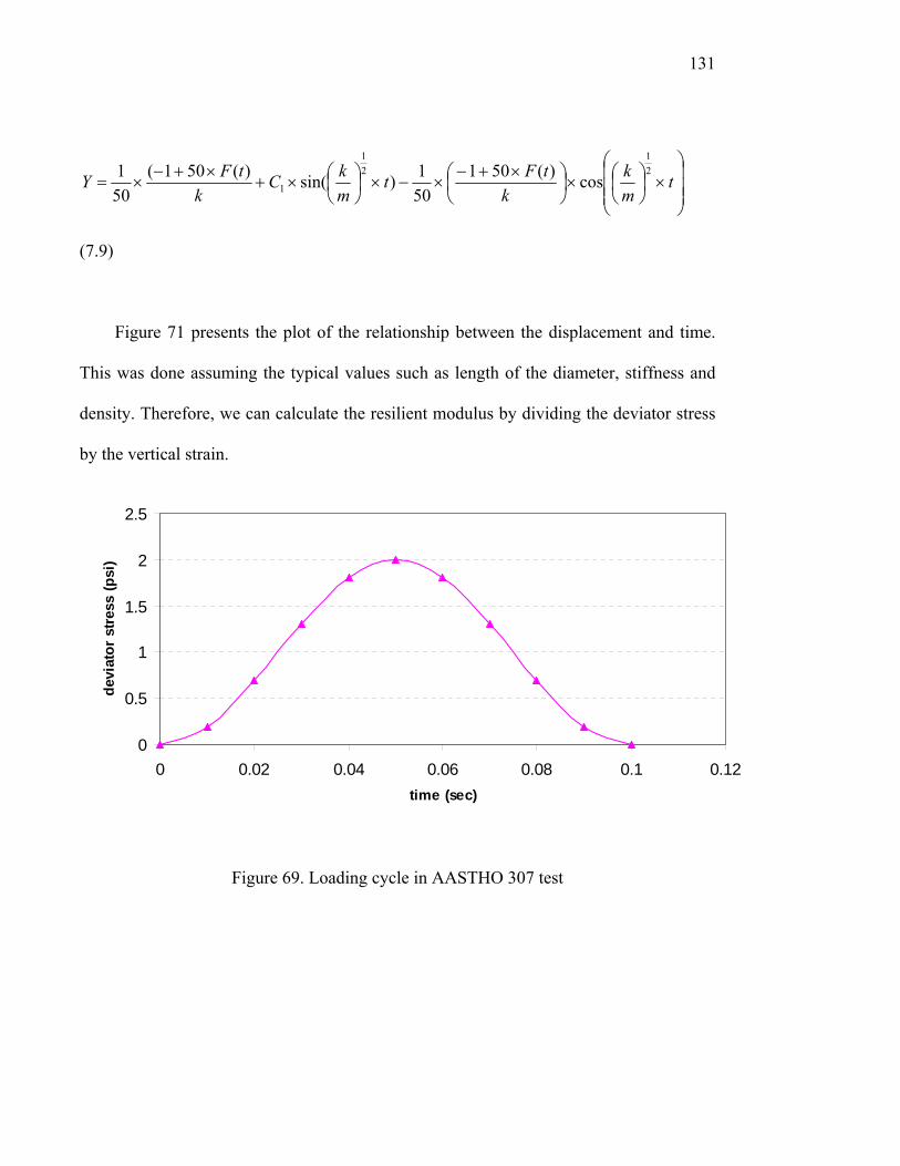
131
⎟⎟⎟
⎠
⎞
⎜⎜⎜
⎝
⎛×⎟
⎠⎞
⎜⎝⎛×⎟
⎠⎞
⎜⎝⎛ ×+−
×−×⎟⎠⎞
⎜⎝⎛×+
×+−×= t
mk
ktFt
mkC
ktFY
21
21
1 cos)(501501)sin()(501(
501
(7.9)
Figure 71 presents the plot of the relationship between the displacement and time.
This was done assuming the typical values such as length of the diameter, stiffness and
density. Therefore, we can calculate the resilient modulus by dividing the deviator stress
by the vertical strain.
0
0.5
1
1.5
2
2.5
0 0.02 0.04 0.06 0.08 0.1 0.12time (sec)
devi
ator
stre
ss (p
si)
Figure 69. Loading cycle in AASTHO 307 test
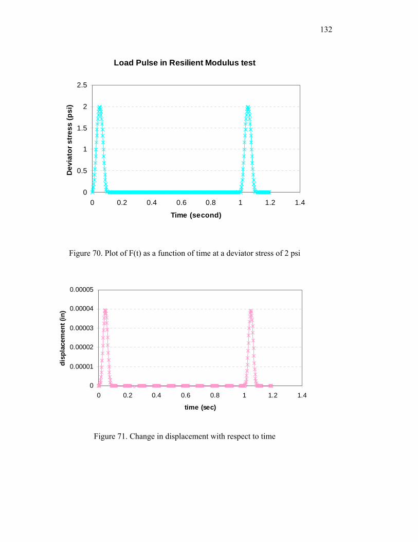
132
Load Pulse in Resilient Modulus test
0
0.5
1
1.5
2
2.5
0 0.2 0.4 0.6 0.8 1 1.2 1.4
Time (second)
Dev
iato
r str
ess
(psi
)
Figure 70. Plot of F(t) as a function of time at a deviator stress of 2 psi
0
0.00001
0.00002
0.00003
0.00004
0.00005
0 0.2 0.4 0.6 0.8 1 1.2 1.4
time (sec)
disp
lace
men
t (in
)
Figure 71. Change in displacement with respect to time
133
7.2. Development of a Constitutive Model for a soil having Permanent Strain Subjected
to the Resilient Modulus Test
Generally, the permanent strain of subgrade soils is not taken into consideration in
the resilient modulus test. This is due to the assumption that the subgrade would be in the
elastic state. However, as discussed previously, subgrade soils may exhibit the permanent
strain even at a much smaller load than that causing shear failure. It is fairly necessary to
develop a constitutive model that describes the realistic behavior of subgrade soils.
The permanent strain at small loads cannot be modeled using classical plasticity
constitutive models such as the Drucker-Prager model or the Mohr-Coulomb model, as
the stress state of soils with those models will always be elastic. In the modeling of
subgrade, as the plastic deformation occurs during the Mr testing, a simple classical
plasticity theory that does not require the shear strength parameters (cohesion and friction
angle) can be employed to consider both the resilient behavior and the permanent
behavior. Soil plasticity consists of the three parts: a yield criterion, a flow rule, and a
hardening rule.
7.2.1. Yield Criterion
A yield function F can be defined as a function of stresses { }σ and Wp associated
with the isotropic hardening rule. Yielding occurs when the following condition is
satisfied:
134
0),( =PWF σ (7.10)
Where { } { }pTp dW εσ∫= = plastic work (7.11)
Throughout this paper, {} is defined as a column matrix and [] is as a rectangular or a
square matrix.
7.2.2. Flow Rule
We define a plastic potential Q, which has units of stress and is a function of stresses,
),( pWQQ σ= . With dλ, a scalar called plastic multiplier, plastic strain increments are
given by:
{ } λσ
ε dQd p
⎭⎬⎫
⎩⎨⎧∂∂
= (7.12)
An incremental stress-strain, analogous to the relation { } [ ]{ }εσ C= of elasticity but
valid into the elasto-plastic regime, can be derived as follows. [ ]C is a three-dimensional
elastic tangent stiffness matrix, which is symmetric, as given by:
135
[ ]
⎥⎥⎥⎥⎥⎥⎥⎥⎥⎥
⎦
⎤
⎢⎢⎢⎢⎢⎢⎢⎢⎢⎢
⎣
⎡
−
−
−−
−−
−+=
2)21(00000
02
)21(0000
002
)21(000
000)1(000)1(000)1(
)21)(1(
v
v
vvvv
vvvvvv
vvEC (7.13)
Differentiation of eq. (7.10) leads to
{ } 0=∂∂
+⎭⎬⎫
⎩⎨⎧∂∂
= PP
T
dWWFdFdF σ
σ (7.14)
From eq. (7.11) { } { }pTp ddW εσ=
{ } [ ]{ } [ ]{ } { }( )pe ddCdCd εεεσ −== (7.15)
Plugging (12) into (15) and rearranging (15) in terms of dλ becomes:
{ } { }ελ dDd T= (7.16)
where { }[ ]
[ ] { }⎭⎬⎫
⎩⎨⎧∂∂
∂∂
−⎭⎬⎫
⎩⎨⎧∂∂
⎭⎬⎫
⎩⎨⎧∂∂
⎭⎬⎫
⎩⎨⎧∂∂
=
σσ
σσ
σQ
WFQCF
CF
DT
P
T
T
T (7.17)
Finally, substituting eq. (7.12) into eq. (7.15) gives:

136
{ } [ ] { } ⎟⎟⎠
⎞⎜⎜⎝
⎛⎭⎬⎫
⎩⎨⎧∂∂
−= λσ
εσ dQdCd or { } [ ]{ }εσ dCd ep= (7.18)
where [ ] [ ] [ ] { }Tep DQCCC
⎭⎬⎫
⎩⎨⎧∂∂
−=σ
= elasto-plastic tangent stiffness matrix or Jacobian
matrix, [ ]epC = 6×6 matrix, ⎭⎬⎫
⎩⎨⎧∂∂σQ = 6×1 matrix,
TF⎭⎬⎫
⎩⎨⎧∂∂σ
= 1×6 matrix, { }TD = 1×6 matrix,
and { }Tσ = 1×6 matrix.
7.2.3. Implementation Process
1) Material parameters needed: ν, k1, k2 and k3
32
11
k
a
oct
k
aar pp
pkM ⎟⎟⎠
⎞⎜⎜⎝
⎛+⎟⎟
⎠
⎞⎜⎜⎝
⎛=
τθ (7.19)
where 332211 σσσθ ++= and ( ) ( ) ( )2322
312
21(31 σσσσσστ −+−+−=oct
In order to incorporate the non-linearity of resilient behavior of soils, E in equation (7.13)
is substituted by Mr in equation (7.19). Unlike the Mohr-Coulomb or the Drucker-Prager
model, the yield criterion requires only a hardening rule, and hence the stress-strain
relation obtained from a resilient modulus test is sufficient to model both the resilient and
the permanent behavior of a soil.
2) Failure criterion The yield criterion determines the stress level at which plastic deformation begins and
can be written in the general form:

137
F(σ, Wp) =q(σ)-g(Wp) = 0 (7.20)
where q = Mises equivalent stress
)}(6)()(){(212/3 2
132
232
122
11332
33222
2211 σσσσσσσσσ +++−+−+−== ijijSSq
and 028.17)ln(4687.1)( += WpWg p
)4687.1
028.17exp(
4687.1−
=∂∂
dpWF
σ
As shown above, the hardening rule is dependent on the deviator stress. The effect of the
number of repeated loading is internally taken into account. The hardening rule is based
on the long-term resilient modulus test data for Orchard clay.
3) Assuming the associate flow rule, ⎭⎬⎫
⎩⎨⎧∂∂
=⎭⎬⎫
⎩⎨⎧∂∂
σσFQ
)2()}(6))()(){(
212
1332211
213
223
212
21133
23322
22211
11
σσσσσσσσσσσσ
σ−−
+++−+−+−=
∂∂F
)2()}(6))()(){(
212
132211
213
223
212
21133
23322
22211
22
σσσσσσσσσσσσ
σ−+−
+++−+−+−=
∂∂F
)2()}(6))()(){(
212
132211
213
223
212
21133
23322
22211
33
σσσσσσσσσσσσ
σ+−−
+++−+−+−=
∂∂F
138
)6()}(6))()(){(
212
112
213
223
212
21133
23322
22211
12
σσσσσσσσσσ
σ+++−+−+−
=∂∂F
)6()}(6))()(){(
212
113
213
223
212
21133
23322
22211
13
σσσσσσσσσσ
σ+++−+−+−
=∂∂F
)6()}(6))()(){(
212
123
213
223
212
21133
23322
22211
23
σσσσσσσσσσ
σ+++−+−+−
=∂∂F
The constitutive model discussed above was implemented in ABAQUS, a general
Finite Element (FE) program, to account for both the resilient behavior and the
permanent strain behavior. The detailed program code for user material is provided in
Appendix. For a simple Finite Element (FE) analysis, a sample with a height of 6.0” and
a diameter of 2.8” for a resilient modulus test was modeled as axis-symmetric condition.
The sample is subjected to a confining stress of 2 psi and deviator stress of 6 psi. As
discussed previously, when modeling this specimen with the Drucker-Prager or the
Mohr-Coulomb model, the permanent strain will not occur. Figure 72 shows the
comparison between measured and predicted permanent strains induced by 10 times of
the repeated loading. It is observed from Figure 72 that the measured permanent strain
caused by the first loading is larger than that from the FE analysis. This results from the
incomplete contact of the sample at the first loading. As the loading continues, the total
magnitude of permanent strain increases with the decrease in the rate of permanent strain
in each loading cycle. This agrees well with the observation from a resilient modulus test,
as the specimen is compacted due to the continued loading. As can be seen in Figure 72,
the measured and predicted Mr values are reasonably in good agreement.
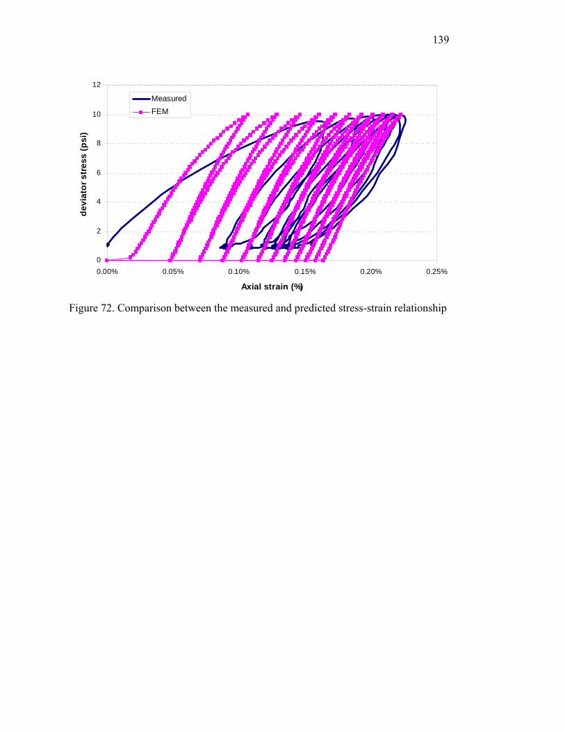
139
0
2
4
6
8
10
12
0.00% 0.05% 0.10% 0.15% 0.20% 0.25%
Axial strain (%)
devi
ator
str
ess
(psi
)
Measured FEM
Figure 72. Comparison between the measured and predicted stress-strain relationship
140
CHAPTER 8. CONCULUSIONS AND RECOMMENDATION
8.1. Conclusions
The objectives of this study were to simplify the resilient modulus testing procedure
specified in AASHTO T307 based on the prevalent conditions in Indiana, to generate
database of Mr values following the existing resilient modulus test method (AASHTO
T307) for Indiana subgrades, to develop useful predictive models for use in Level 1 and
Level 2 input of subgrade Mr values following the New M-E Design Guide, to develop a
simple calculation method, and to develop a constitutive model based on the Finite
Element Method (FEM) to account for both the resilient and permanent behavior of
subgrade soils. The following conclusions can be drawn from this study.
1) Resilient modulus test results showed that it may be possible to simplify the
complex procedures required in the existing Mr testing (AASHTO T307) to a
single step with a confining stress of 2 psi and deviator stresses of 2, 4, 6, 8, 10
and 15 psi. The simplified procedure suggested compared well with the
existing Mr testing procedure. The simplified procedure can be used for
estimation of resilient modulus rather than performing the complex procedure
with good accuracy. However, it should be noted that one of the disadvantages
to use the simplified procedure is that it considers only one confining stress
level that is the most conservative. If automatic equipment were available, it
would be more desirable to use the wide range of stresses in existing standard

141
resilient modulus test. This is because the additional steps do not require
additional efforts to prepare the specimen and measure the data, and a number
of data can be obtained to use different stress levels.
2) For some soils, excessive permanent strains occurred during resilient modulus
testing. It turns out that this is because the stress ratio of the deviator stress to
the peak strength of those soils and the permanent strains to reach the peak
strengths were significant large.
3) The current Mr testing uses the original length of the specimen, but it is
recommended that the deformed length during testing be used for more
accurate calculation of Mr.
4) The largest Mr values are observed in the Dry samples for silty sandy clay soils
due to the capillary suction while the largest Mr values are observed either in
the Dry or OMC sample for clay soils. The smallest Mr values obtained from
Wet samples. The resilient modulus for Wet samples can be used as the limit of
Mr in spring and further study needs to be done.
5) Three predictive models based on unconfined compressive tests, and resilient
modulus tests were developed for use in subgrade design inputs. Comparisons
of predicted moduli with measured ones show satisfactory agreement. These
predictive models can be used for the estimation of design resilient modulus
inputs for Level 1 or Level 2 design inputs.
6) A predictive model to estimate material coefficients k1, k2, and k3 using 12 soil
variables obtained from the soil property tests and the standard Proctor tests
was developed. The predicted resilient moduli using all the predictive models

142
compared satisfactorily with measured ones. These predictive models can be
used for the estimation of design resilient modulus inputs for Level 1 or Level
2 design inputs.
7) A mathematical expression using Fourier series for the repeated loading on a
soil was derived and this can be used as a simple calculation for obtaining the
resilient modulus;
8) Although the permanent strain occurs during the resilient modulus test, the
permanent behavior of subgrade soils is currently not taken into consideration.
In order to capture both the permanent and the resilient behavior of subgrade
soils, a constitutive model based on the Finite Element Method (FEM) was
proposed. The predictive permanent strains are comparable to the measured
ones. The proposed constitutive model can allow capturing the permanent
behavior of subgrade soils subjected to a much smaller load (e.g. the load used
in resilient modulus testing) than that causing shear failure, which cannot be
modeled by classical constitutive models such as the Mohr-Coulomb or the
Drucker-Prager model. A comparison of the measured permanent strains with
those obtained from the Finite Element (FE) analysis showed a reasonable
agreement.
9) The current Mr testing cannot take into account the long term Mr values due to
a limited number of repeated loadings applied to the specimen. The long term
Mr values are especially needed for rehabilitation. The long-term resilient
modulus tends to level off after 5,000 repetitions of repeated loading and the
long-term permanent strain tends to plateau under a consistent stress level,

143
often after approximately 500 repetitions. This supports the number of the
repetitions of the conditioning stage used for the standard resilient modulus test,
however it is likely that soil may experience a different plateau under a
different stress condition.
10) An extensive review of the M-E design for subgrades was done. Based on the
test results and review of the M-E Design, implementation initiatives can be
proposed in the next section.
8.2. Implementation of Unbound Material Design Inputs
8.2.1. Subgrade Design Input Level 3
In Level 3 design, a modulus value for unbound material is required. There are two
options to determine the modulus: ICM Calculated Modulus, and User Input Modulus
(i.e., Representative Modulus). The ICM Calculated Modulus allows seasonal variation in
the moduli for different months while the User Input Modulus remains constant for the
entire design period. Therefore, it is desirable to use the ICM input module. In addition, a
general equation between the Mr and CBR values is provided. Typical CBR values for
most of untreated fine-grained soils in Indiana are in the range of 3 to 15% corresponding
to Mr values from 4,940 to 12,970 psi. This range of Mr appears to be reasonable in the
design input Level 3.
8.2.2. Subgrade Design Input Level 2
In Level 2 design, the following properties: Mr, CBR, R-value, Dynamic Cone
Penetration Test (DCPT), layer coefficient and Plasticity Index (PI) and gradation can be
144
selected. As discussed earlier, there are two design input options: EICM input and
representative Mr input, and seasonal input. Several analyses revealed that similar
outputs are observed in both Level 3 and Level 2 when a resilient modulus is selected
using the Integrated Climatic Model (ICM) module. For seasonal design input option,
monthly resilient moduli are required.
For Level 2 design, as shown previously, the following equation based on the results
of unconfined compressive tests can be used.
Mr = 11267.7×ln(Et)+3217.239×ln(qu)-76.9/ εy + -8725.31×ln(Ef) 2587.73×ln(qy)
+127.5/εy - 13513.9 (8.1)
Where E = tangent elastic modulus, qu = unconfined compressive strength, Ef = Secant
modulus at failure, εy = strain at yield stress, Mr = Resilient modulus at a confining stress
of 2 psi and a deviator stress of 6 psi.
All the tested soils were prepared at dry of optimum (95% of the maximum dry
density), optimum, and wet of optimum (95% of the maximum dry density). As shown in
Figure 40, predicted resilient moduli using equation (8.1) were reasonably comparable
with the measured resilient moduli. When State DOTs are not capable of performing a
resilient modulus test, this type of equation based on the unconfined compressive test
would be quite useful to predict the resilient modulus.
145
8.2.3. Subgrade Design Input Level 1
In Level 1 design, non-linear coefficients k1, k2, and k3 are required. In order to
generate a Mr predictive model, testing data for fourteen compacted cohesive subgrade
soils were analyzed. As discussed previously, the following non-linear regression
coefficients were obtained.
Log k1=6.660876 - 0.22136 x OMC - 0.04437 x MC - 0.92743 x MCR - 0.06133 x DD +
10.64862 x %COMP + 0.328465 x SATU - 0.04434 x %SAND - 0.04349 x
%SILT - 0.01832 x %CLAY + 0.027832 x LL - 0.01665 x PI
k2=3.952635 - 0.33897 x OMC + 0.076116 x MC - 2.45921 x MCR - 0.06462 x DD +
6.012966 x %COMP + 1.559769 x SATU + 0.020286 x %SAND + 0.002321 x
%SILT + 0.011056 x %CLAY + 0.077436 x LL - 0.05367 x PI
k3=2.634084 + 0.124471 x OMC - 0.09277 x MC + 0.366778 x MCR - 0.01168 x DD -
1.32637 x %COMP + 1.297904 x SATU - 0.01226 x %SAND - 0.00512 x %SILT -
0.00492 x %CLAY - 0.05083 x LL + 0.018864 x PI
(8.2)
where; OMC (Optimum Moisture Content), MC (Moisture Content), MCR (Moisture
Content Ratio = Moisture Content/ Optimum Moisture Content), DD (Dry Density),
%COMP (Percent Compaction = Dry Density/ Maximum Dry Density), SATU (Degree
of Saturation), %SAND (Percent Sand in Particle Size Distribution Curve), %SILT

146
(Percent Silt in Particle Size Distribution Curve), %CLAY (Percent Clay in Particle Size
Distribution Curve), LL (Liquid Limit) and PI (Plasticity Index).
The resilient modulus can be calculated by inserting the regression coefficient into
the following equation (8.3) which is recommended by M-E Design Guide (NCHRP
2004):
32 )1()(1k
a
octk
aa pp
pkMr +=τθ (8.3)
where, k1, k2, k3, = regression coefficients; θ = sum of principal stresses; pa = reference
pressure = 100 kpa ≈ 1 kgf/cm2 ≈ 2000 psf ≈ 14.5 psi; σd = deviator stress in the same
unit as pa, and τoct is the octahedral shear stress.
If a resilient modulus testing can be done, it is the best way to obtain the nonlinear
regression coefficients through a laboratory Mr test data obtained from AASHTO T 307.
8.2.4. Design Example – Level 1, Level 2
Two design examples are presented in the following case studies. A pavement
section consists of 4 inches of hot-mix asphalt surface and intermediate layers, 3 inches
of hot-mix asphalt permeable base, 3 inches of hot-mix asphalt base layer on 24 inches of
subgrade layer, and a semi-infinite layer, top to bottom. The pavement location is in
Northwest Indiana and the climatic data available for South Bend station were selected.
In order to design the subgrade, the following physical and mechanical tests are
needed: sieve analysis, Atterberg limit tests, compaction test, unconfined compressive

147
tests on samples compacted at OMC and wet of optimum, resilient modulus tests on
samples compacted at OMC and wet of optimum. The results of the subgrade soil are
presented from Figure 73 to Figure 77 and in Table 8.
0
20
40
60
80
100
0.0010.010.1110100Grain size, D(mm)
Perc
ent f
iner
Figure 73. Particle size distributions
Table 8. Material properties for a design example soil %
Gravel % Sand
% Silt
% clay LL PI AASHTO USCS
#4soil 2.5 23.2 59.8 14.5 43 21 A-7-6 CL
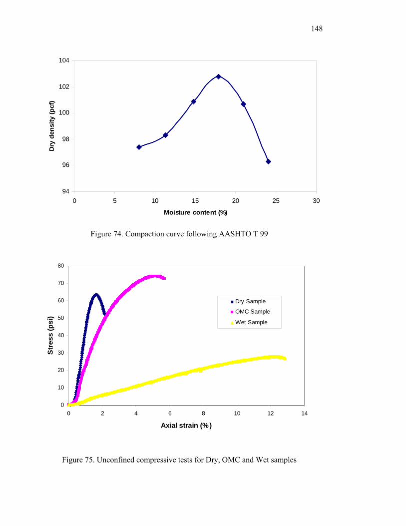
148
94
96
98
100
102
104
0 5 10 15 20 25 30
Moisture content (%)
Dry
dens
ity (p
cf)
Figure 74. Compaction curve following AASHTO T 99
0
10
20
30
40
50
60
70
80
0 2 4 6 8 10 12 14
Axial strain (%)
Stre
ss (p
si)
Dry Sample
OMC Sample
Wet Sample
Figure 75. Unconfined compressive tests for Dry, OMC and Wet samples

149
0
3000
6000
9000
12000
15000
0 3 6 9 12
Deviator stress (psi)
Mr (
psi)
Conf. = 6 psiConf. = 4 psiConf. = 2 psi
Figure 76. Resilient modulus test for OMC sample following AASHTO T-307
0
800
1600
2400
3200
4000
0 3 6 9 12
Deviator stress (psi)
Mr (
psi)
Conf. = 6 psiConf. = 4 psiConf. = 2 psi
Figure 77. Resilient modulus test for wet sample following AASHTO T-307
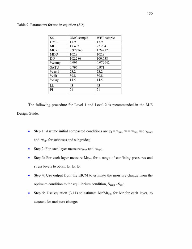
150
Table 9. Parameters for use in equation (8.2)
Soil OMC sample WET sample OMC 17.9 17.9 MC 17.493 22.234 MCR 0.977263 1.242123 MDD 102.8 102.8 DD 102.286 100.738 %comp 0.995 0.979942 SATU 0.797 0.971 %sand 23.2 23.2 %silt 59.8 59.8 %clay 14.5 14.5 LL 43 43 PI 21 21
The following procedure for Level 1 and Level 2 is recommended in the M-E
Design Guide.
• Step 1: Assume initial compacted conditions are γd = γmax, w = wopt, use γdmax
and wopt for subbases and subgrades;
• Step 2: For each layer measure γmax and wopt;
• Step 3: For each layer measure Mropt for a range of confining pressures and
stress levels to obtain k1, k2, k3;
• Step 4: Use output from the EICM to estimate the moisture change from the
optimum condition to the equilibrium condition, Sequil - Sopt;
• Step 5: Use equation (3.11) to estimate Mr/Mropt for Mr for each layer, to
account for moisture change;

151
• Step 6: Account for change in moduli due to freezing, thawing, and recovery
using the recommendations by NCHRP report (2004).
As discussed previously, the M-E Design Guide may lead to unconservative
design for subgrade, the following conservative design procedure is proposed:
• Step 1: To be conservative assume γd = γavg = (γdmax + γwet)/2, w = wavg =
(wopt+wwet)/2, use γavg and wavg for subbases and subgrades. The maximum
dry density and dry density corresponding to wet of optimum (95% of γdmax)
and optimum moisture content and moisture content for wet of optimum can
be obtained from compaction curve shown in Figure 74. These are γdmax =
102.8 pcf, γwet = 97.66 pcf, γavg = 100.23 pcf, wopt = 17.9 %, wwet = 24 %
and wavg = 20.95 %;
• Step 2: For each layer determine γavg and wavg. Use the values obtained above;
• Step 3: For each layer measure Mravg = (Mropt+Mrwet)/2 for a range of
confining pressures and stress levels to obtain k1, k2, k3 or use equation (8.2)
based on the soil properties. Mropt and Mrwet are obtained from Figures 76 and
77. Mravg = 6, 207 psi, Mropt = 9, 855 psi, and Mrwet = 2, 559 psi for a
confining stress of 2 psi and a deviator stress of 6 psi are obtained using
equation (8.2) based on the soil parameters shown in Table 9. When a resilient
modulus test is not available, perform an unconfined compressive test as
shown in Figure 75;
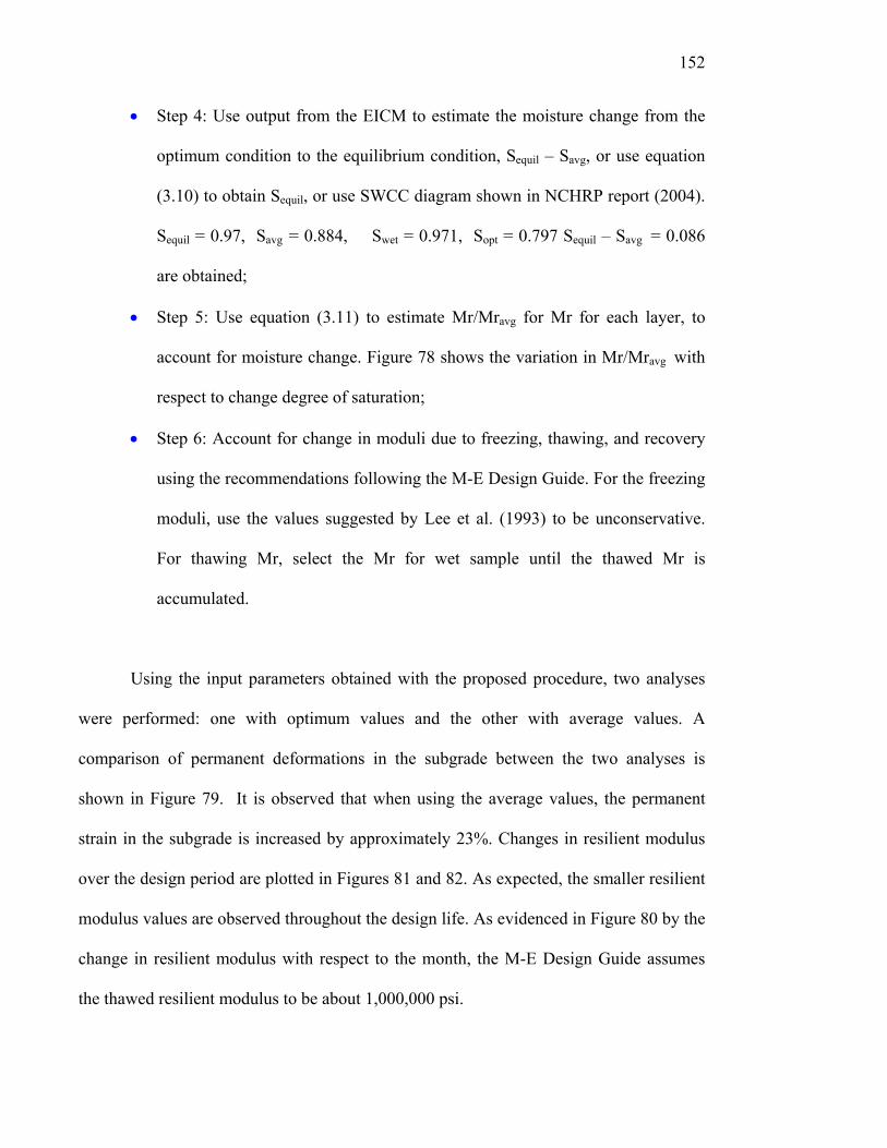
152
• Step 4: Use output from the EICM to estimate the moisture change from the
optimum condition to the equilibrium condition, Sequil – Savg, or use equation
(3.10) to obtain Sequil, or use SWCC diagram shown in NCHRP report (2004).
Sequil = 0.97, Savg = 0.884, Swet = 0.971, Sopt = 0.797 Sequil – Savg = 0.086
are obtained;
• Step 5: Use equation (3.11) to estimate Mr/Mravg for Mr for each layer, to
account for moisture change. Figure 78 shows the variation in Mr/Mravg with
respect to change degree of saturation;
• Step 6: Account for change in moduli due to freezing, thawing, and recovery
using the recommendations following the M-E Design Guide. For the freezing
moduli, use the values suggested by Lee et al. (1993) to be unconservative.
For thawing Mr, select the Mr for wet sample until the thawed Mr is
accumulated.
Using the input parameters obtained with the proposed procedure, two analyses
were performed: one with optimum values and the other with average values. A
comparison of permanent deformations in the subgrade between the two analyses is
shown in Figure 79. It is observed that when using the average values, the permanent
strain in the subgrade is increased by approximately 23%. Changes in resilient modulus
over the design period are plotted in Figures 81 and 82. As expected, the smaller resilient
modulus values are observed throughout the design life. As evidenced in Figure 80 by the
change in resilient modulus with respect to the month, the M-E Design Guide assumes
the thawed resilient modulus to be about 1,000,000 psi.
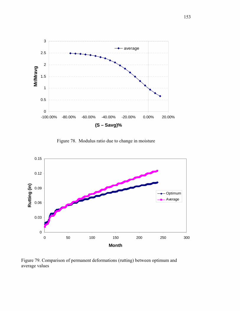
153
0
0.5
1
1.5
2
2.5
3
-100.00% -80.00% -60.00% -40.00% -20.00% 0.00% 20.00%
(S – Savg)%
Mr/M
ravg
average
Figure 78. Modulus ratio due to change in moisture
0
0.03
0.06
0.09
0.12
0.15
0 50 100 150 200 250 300
Month
Rut
ting
(in)
OptimumAverage
Figure 79. Comparison of permanent deformations (rutting) between optimum and average values
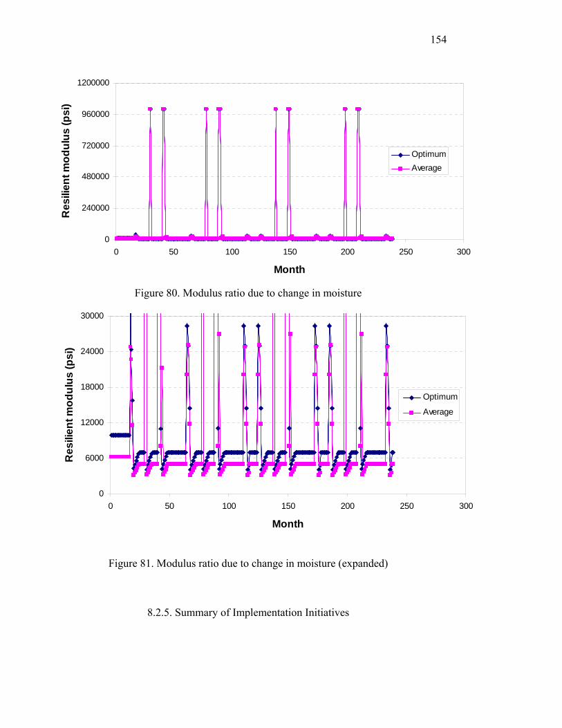
154
0
240000
480000
720000
960000
1200000
0 50 100 150 200 250 300
Month
Res
ilien
t mod
ulus
(psi
)
OptimumAverage
Figure 80. Modulus ratio due to change in moisture
0
6000
12000
18000
24000
30000
0 50 100 150 200 250 300
Month
Res
ilien
t mod
ulus
(psi
)
Optimum
Average
Figure 81. Modulus ratio due to change in moisture (expanded)
8.2.5. Summary of Implementation Initiatives

155
With the advent of the new M-E Design Guide, highway agencies are encouraged
to implement an advanced design following its philosophies. As part of implementation
of the M-E Design Guide, the present study reviewed the features embedded in this new
design guide for unbound materials, especially subgrades.
The following can be summarized:
• The M-E Design Guide assumes that the subgrade is compacted to optimum
moisture content, leading to unconservative design. In order to ensure a
conservative design for subgrades, the use of the average values is
recommended (to be more conservative, use of the Mr at wet of optimum may
be possible);
• When laboratory testing for evaluating thawed Mr is not available, the use of
Mr for wet of optimum would be reasonable;
• Caution needs to be taken to use the conservative frozen Mr value suggested
in M-E Design Guide.
• In characterizing subgrade in Indiana, Mr testing program for both design
inputs Level 2 and Level 1 is desirable.
8.3. Recommendations
1) In this study, the resilient and permanent behavior of cohesive subgrade was
mainly investigated. Further study on resilient behavior of cohesionless subgrade
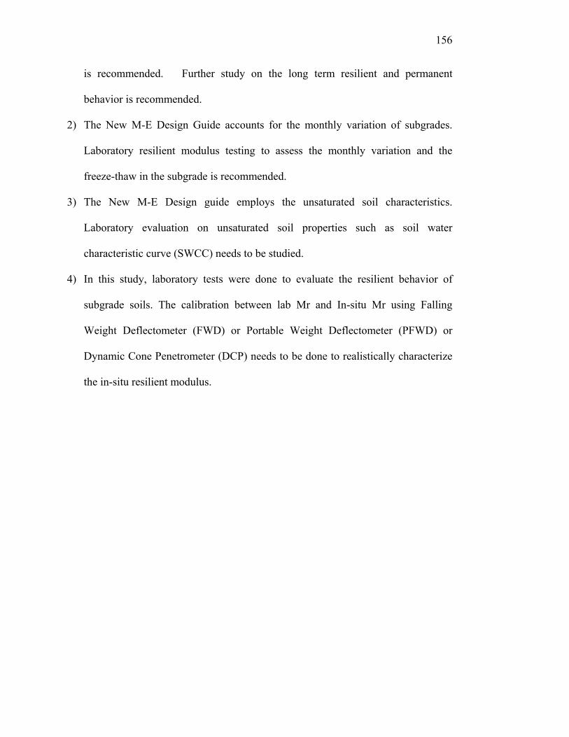
156
is recommended. Further study on the long term resilient and permanent
behavior is recommended.
2) The New M-E Design Guide accounts for the monthly variation of subgrades.
Laboratory resilient modulus testing to assess the monthly variation and the
freeze-thaw in the subgrade is recommended.
3) The New M-E Design guide employs the unsaturated soil characteristics.
Laboratory evaluation on unsaturated soil properties such as soil water
characteristic curve (SWCC) needs to be studied.
4) In this study, laboratory tests were done to evaluate the resilient behavior of
subgrade soils. The calibration between lab Mr and In-situ Mr using Falling
Weight Deflectometer (FWD) or Portable Weight Deflectometer (PFWD) or
Dynamic Cone Penetrometer (DCP) needs to be done to realistically characterize
the in-situ resilient modulus.
157
LIST OF REFERENCES “The AASHO Road Test”. (1962). Report 7, American Association of State High Officials, Washington, D.C. Bergado D. T., Anderson, L. R., Miura, N. and Balasubramaniam, A. S. (1996). “Soft Ground Improvement in Lowland and Other Environments”, ASCE, New York. Chen, W. F. and Saleeb, A. F. (1994). “Constitutive Equations for Engineering Materials”, Vol. 2, Elsevier Science B.V, Amsterdam, The Netherlands. Cook, R. D., Malkus, D. S. and Plesha, M. E. (1989). “Concepts and Applications of Finite Element Analysis, 3rd edition, John Wiley & Sons. Daita, R. C., Drnevich, V., Kim, D. (2005). “Family of Compaction Curves for Chemically Modified Soils”, M.S Thesis, Purdue University, West Lafayette, IN. Desai, C. C. and Siriwardane, H. J. (1984). “Constitutive Laws for Engineering Materials with Emphasis on Geological Materials, Prentice-Hall, Englewood Cliffs, New Jersey. Diyaljee, V. A. and Raymond, G. P. (1983). “Repetitive Load Deformation of Cohesionless Soil”, Journal of Geotechnical and Engineering, ASCE, Vol. 108, No. 10, pp. 1215-1229. Drumm, E. C., Boateng-Poku, Y. and Pierce, T. J. (1990). “Estimation of Subgrade Resilient Modulus from Standard Tests.” Journal of Geotechnical Engineering, ASCE, Vol. 116, No. 5, pp. 774-789. Drumm, E. C., Reeves, J. S., Madgett, M.R. and Trolinger, W. D. (1997). “Subgrade Resilient Modulus Correction for Saturation Effects.” Journal of Geotechnical and Geoenvironmental Engineering, ASCE, Vol. 123, No. 7, pp. 663-670. Elliott, R. P., and Thornton, S. I. (1988). “Resilient Modulus and AASHTO Pavement Design.” Transportation Research Record, 1196, TRB, National Research Council, Washington, D.C., pp. 116-124.

158
Elliott, R. P., Dennis, N. and Qiu, Y. (1999). “Permanent Deformation of Subgrade Soils, Phase II: Repeated Load Testing of Four Soils.” Report No. MBTC FR-1089, Final Report, National Technical Information Service, Springfiled, VA, pp.1-85. Gaskin, P. N., Raymond, G. P. and Addo-Abedi, F. Y. (1979). “Repeated Compressive Loading of a Sand”. Canadian Geotechnical Journal, National Research Council of Canada, Vol. 16, pp. 798-802. Ghazzaly, O. and Ha, H. (1975). “Pore Pressures and Strains After Repeated Loading of Saturated Clay: Discussion.” Canadian Geotechnical Journal. National Research Council of Canada, Vol. 12, pp. 265-267. Hall, D. K. and Thompson, M. R. (1994). “Soil-Property-Based Subgrade Resilient Modulus Estimation for Flexible Pavement Design.” Transportation Research Record, 1449, TRB, National Research Council, Washington, D.C., pp. 30-38. Hardin, B. O. and Black, W. L (1968). “Vibration Modulus of Normally Consolidted Clay”, Journal of Soil Mechanics and Foundation Engineering Division, ASCE, 94(SM2), pp. 353-369. Hardin, B. O. and Drnevich, V. P. (1972). “Shear Modulus and Damping in soils; Design Equations and Curves”, Journal of Soil Mechanics and Foundations Divisions, ASCE, 98(7), pp. 667-692. Hausmann, M. R. (1990). “Engineering Principles of Ground Modification”, McGraw-Hill Publishing Company. Hicks, R. G., and Monismith, C. L. (1971). “Factors Influencing the Resilient Response of Granular Materials”. Highway Research Record 345, Highway Research Board, Washington, D.C., pp. 15-31. Huang, Y. H. (1993). “Pavement Analysis and Design”, Prentice Hall, Englewood Cliffs, N.J. Hyde, A. F. L. (1974). “Repeated load triaxial testing of soils”.. Ph.D. Thesis, University of Notingham, U.K.. Indiana State. (2005). “Indiana Specification”. Kim, D. (2002). “Effects of Supersingle Tire Loadings on Subgrades’, Ph. D thesis, Purdue University, West Lafayette, IN. Kim, D. and Siddiki, N. Z. (2004). “Lime Kiln Dust-Lime – A Comparative Study in Indiana, Transportation Research Board, Washington D. C.
159
Ladd, C. C., Foote, R., Ishihara, K., Schlosser, F. and Poulos, H. G. (1977). “Stress Deformation and Strength Characteristics”, Proc., of 9th International Conference on Soil Mechanics and Foundation Engineering, Tokyo, Vol. 2, pp. 421-494. Lee, W. (1993). “Evaluation of In-Service Subgrade Resilient Modulus with Consideration of Seasonal Effects”, Ph.D. Thesis, Purdue University, West Lafayette, IN. Lee, W. J., Bohra, N. C., Altschaeffl, A. G. and White, T. D. (1997). “Resilient Modulus of Cohesive Soils”, Journal of Geotechnical and Geoenvironmental Engineering, ASCE, Vol. 123, No. 2, pp. 131-136. Lee, W., Bohra, N. C. and Altschaeffl, A.G. (1995). “Resilient Characteristics of Dune Sand”, Journal of Transportation Engineering, ASCE, Vol. 121, No. 6, pp. 502-506. Lekarp, F., Isacsson, U. and Dawson, A. (2000). “State of The Art. I: Resilient Response of Unbound Aggregates”, Journal of Transportation Engineering, Vol. 126, pp.66-75. Lekarp, F. and Dawson, A. (1998). “Modeling Permanent Deformation Behavior of Unbound Granular Materials”, Construction and Building Materials, Elsevier Science Ltd, Vol. 12, No. 1, pp. 9-18. Lekarp, F., Isacsson, U. and Dawson, A. (2000). “State of The Art. II: Permanent Strain of Unbound Aggregates”, Journal of Transportation Engineering, Vol. 126, pp.76-83. Lentz, R.W. and Baladi, G.Y. (1981). “Constitutive Equation for Permanent Strain of Sand Subjected to Cyclic Loading.” Pumphrey, N.D. Jr., and Lentz, R.W.. “Deformation Analyses of Florida Highway Subgrade Sand Subjectd to Repeated Load Triaxial Tests”, Transportation Research Record, 810, TRB, National Research Council, Washington, D.C., 1986, pp. 50-54. Mohammad, L. N., Titi, H. H. and Herath, A. (1999). “Evaluation of Resilient Modulus of Subgrade Soil by Cone Penetration Test”, Transportation Research Record, 1652, TRB, National Research Council, Washington, D.C., pp. 236-245. Mohammad, L. N., Puppala, A. J. and Alavilli, P. (1995). “Resilient Properties of Laboratory Compacted Subgrade Soils”, Transportation Research Record, 1196, TRB, National Research Council, Washington, D.C., pp. 87-102. Monismith, C. L., Ogawa, N. and Freeme, C.R. (1975). “Permanent Deformation Characteristics of Subgrade Soils Due to Repeated Loading”, Transportation Research Record, 537, TRB, National Research Council, Washington, D.C., pp. 1-17.

160
Muhanna, A. S., Rahman, M. S., and Lambe, P. C. (1998). “Model for Resilient Modulus and Permanent Strain of Subgrade Soils”, Transportation Research Record, 1619, TRB, National Research Council, Washington, D.C., pp. 85-93. Pezo, R. F., Kim, D., Stokoe, K. H. II. and Hudson, W. R. (1991). “A Reliable Resilient Modulus Testing System”, Transportation Research Record, 1307, TRB, National Research Council, Washington, D.C., 1990, pp. 90-98. Pezo, R. and Hudson, W. R. (1994). “Prediction Models of Resilient Modulus for Nongranular Materials”, Geotechnical Testing Journal, Vol. 17, No. 3, pp. 349-355. Poulsen, J. and Stubstad, R. N. (1978). “Laboratory Testing of Cohesive Subgrades: Results and Implications Relative to Structural Pavement Design and Distress Models”, Transportation Research Record, 671, TRB, National Research Council, Washington, D.C., pp. 84-91. Pumphrey, N. D. Jr. and Lentz, R. W. (1986). “Deformation Analyses of Florida Highway Subgrade Sand Subjectd to Repeated Load Triaxial Tests”, Transportation Research Record, 1089, TRB, National Research Council, Washington, D.C., pp. 49-56. Puppala, A. J., Mohammad, L. N. and Allen, A. (1996). “Non-Linear Models for Resilient Modulus Characterization of Granular Soils”, Proceedings of Engr. Mechanics, ASCE, New York, N.Y., USA, Vol. 1, pp. 559-562. Raad, L. and Zeid, B.A. (1990). “Repeated Load Model for Subgrade Soils: Model Development”, Transportation Research Record, 1278, TRB, National Research Council, Washington, D.C., pp. 72-82. Raymond, G. P., Gaskin, P. N. and Addo-Abedi, F. Y. (1979). “Repeated Compressive Loading of Leda Clay”, Canadian Geotechnical Journal. National Research Council of Canada, Vol. 16, pp. 1-10. Salgado, R. (1995). “Analysis of Penetration Resistance in Sand”, Ph.D. Thesis, Univ. of California, Berkeley, California. Salgado, R., Bandini, P. and Karim, A. (1999). “Stiffness and Strength of Silty Sand”, Journal of Geotechnical and Geoenvironmental Engineering, ASCE, 126(5), pp. 451-462. Seed, H. B. and Chan, C.K. (1959). “Structure and Strength Characteristics of Compacted Clays”, Journal of Soil Mechanics and Foundation Engineering Division, ASCE, Vol. 85, No. 5, pp. 87-128. Seed, H. B. and Chan, C.K. (1957). “Thixotropic Characteristics of Compacted Clays”, Journal of Soil Mechanics and Foundation Engineering Division, ASCE, Vol. 83, No. 6, pp. 31-47.
161
Seed, H. B., and Chan, C. K. (1958). “Effect of Stress History and Frequency of Stress Application on Deformation of Clay Subgrades Under Repeated Loading”, Proc., Highway Research Record, Vol. 37, Highway Research Board, Washington, D.C., pp. 555-575. Thompson, M. R. and Robnett, Q.L. (1979). “Resilient Properties of Subgrade Soils.” Journal of Transportation Engineering, ASCE, Vol. 105, No. 1, pp. 71-89. Wilson, B. E., Sargand, S. M., Hazen, G. A., and Green, R. (1990). “Multiaxial Testing of Subgrade”, Transportation Research Record, 1278, TRB, National Research Council, Washington, D.C., pp. 91-95. Wilson, N. E., and Greenwood, J. R. (1974). “Pore Pressures and Strains After Repeated Loading of Saturated Clay.” Canadian Geotechnical Journal, National Research Council of Canada, Vol. 11, pp. 269-277.

162
APPENDIX
USER MATERIAL PROGRAM CODE IN ABAQUS
SUBROUTINE UMAT(STRESS,STATEV,DDSDDE,SSE,SPD,SCD, 1 RPL,DDSDDT,DRPLDE,DRPLDT,STRAN,DSTRAN, 2 TIME,DTIME,TEMP,DTEMP,PREDEF,DPRED,CMNAME,NDI,NSHR,NTENS, 3 NSTATV,PROPS,NPROPS,COORDS,DROT,PNEWDT,CELENT, 4 DFGRD0,DFGRD1,NOEL,NPT,KSLAY,KSPT,KSTEP,KINC) C INCLUDE 'ABA_PARAM.INC' C CHARACTER*80 CMNAME DIMENSION STRESS(NTENS),STATEV(NSTATV), 1 DDSDDE(NTENS,NTENS),DDSDDT(NTENS),DRPLDE(NTENS), 2 STRAN(NTENS),DSTRAN(NTENS),TIME(2),PREDEF(1),DPRED(1), 3 PROPS(NPROPS),COORDS(3),DROT(3,3), 4 DFGRD0(3,3),DFGRD1(3,3) c DIMENSION TERM1(1,6), DOT(1,6), CDQDS(6,1), STEPSM(6,6) real*8 E, Nu, rk1, rk2, rk3 real*8 s11, s22, s33, s12, s13, s23 real*8 pa, sd, toct, finu, MR, gp real*8 d(6,6), daj(6,6), a(6), ps(6), w1(6), w2(6) real*8 z, dfds11, dfds22, dfds33, dfds12, dfds13, dfds23 real*8 s_eff real*8 dpe, s(6) real*8 flag_loading real*8 epi logical debug c --- beginning of executable codes --- debug = .false. c initialize flow rule vector a do i = 1,6 a(i) = 0. end do C C *********************************************************** C C INPUT PARAMETERS FOR USER MATERIAL C
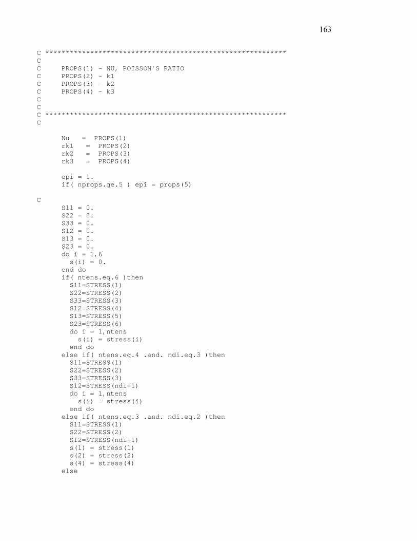
163
C *********************************************************** C C PROPS(1) – NU, POISSON’S RATIO C PROPS(2) – k1 C PROPS(3) – k2 C PROPS(4) – k3 C C C *********************************************************** C Nu = PROPS(1) rk1 = PROPS(2) rk2 = PROPS(3) rk3 = PROPS(4) epi = 1. if( nprops.ge.5 ) epi = props(5) C S11 = 0. S22 = 0. S33 = 0. S12 = 0. S13 = 0. S23 = 0. do i = 1,6 s(i) = 0. end do if( ntens.eq.6 )then S11=STRESS(1) S22=STRESS(2) S33=STRESS(3) S12=STRESS(4) S13=STRESS(5) S23=STRESS(6) do i = 1,ntens s(i) = stress(i) end do else if( ntens.eq.4 .and. ndi.eq.3 )then S11=STRESS(1) S22=STRESS(2) S33=STRESS(3) S12=STRESS(ndi+1) do i = 1,ntens s(i) = stress(i) end do else if( ntens.eq.3 .and. ndi.eq.2 )then S11=STRESS(1) S22=STRESS(2) S12=STRESS(ndi+1) s(1) = stress(1) s(2) = stress(2) s(4) = stress(4) else
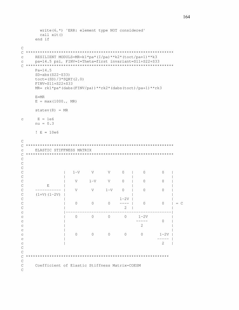
164
write(6,*) 'ERR: element type NOT considered' call xit() end if C C *************************************************************** c RESILIENT MODULS=MR=k1*pa*(I/pa)**k2*(toct/pa+1)**k3 c pa=14.5 psi, FINV=I=Theta=first invariant=S11+S22+S33 C *************************************************************** Pa=14.5 SD=abs(S22-S33) toct=(SD)/3*SQRT(2.0) FINV=S11+S22+S33 MR= rk1*pa*(dabs(FINV/pa))**rk2*(dabs(toct)/pa+1)**rk3 E=MR E = max(1000., MR) statev(8) = MR c E = 1e6 nu = 0.3 ! E = 10e6 C C *************************************************************** c ELASTIC STIFFNESS MATRIX C *************************************************************** C C C C | 1-V V V 0 | 0 0 | C | | | C | V 1-V V 0 | 0 0 | C E | | | C ----------- | V V 1-V 0 | 0 0 | C (1+V)(1-2V) | | | C | 1-2V | | C | 0 0 0 ---- | 0 0 | = C C | 2 | | c |---------------------------------------------| c | 0 0 0 0 1-2V | c | ----- 0 | c | 2 | c | | c | 0 0 0 0 0 1-2V | c | ----- | c | 2 | C C C ************************************************************* C C Coefficient of Elastic Stiffness Matrix=COESM C
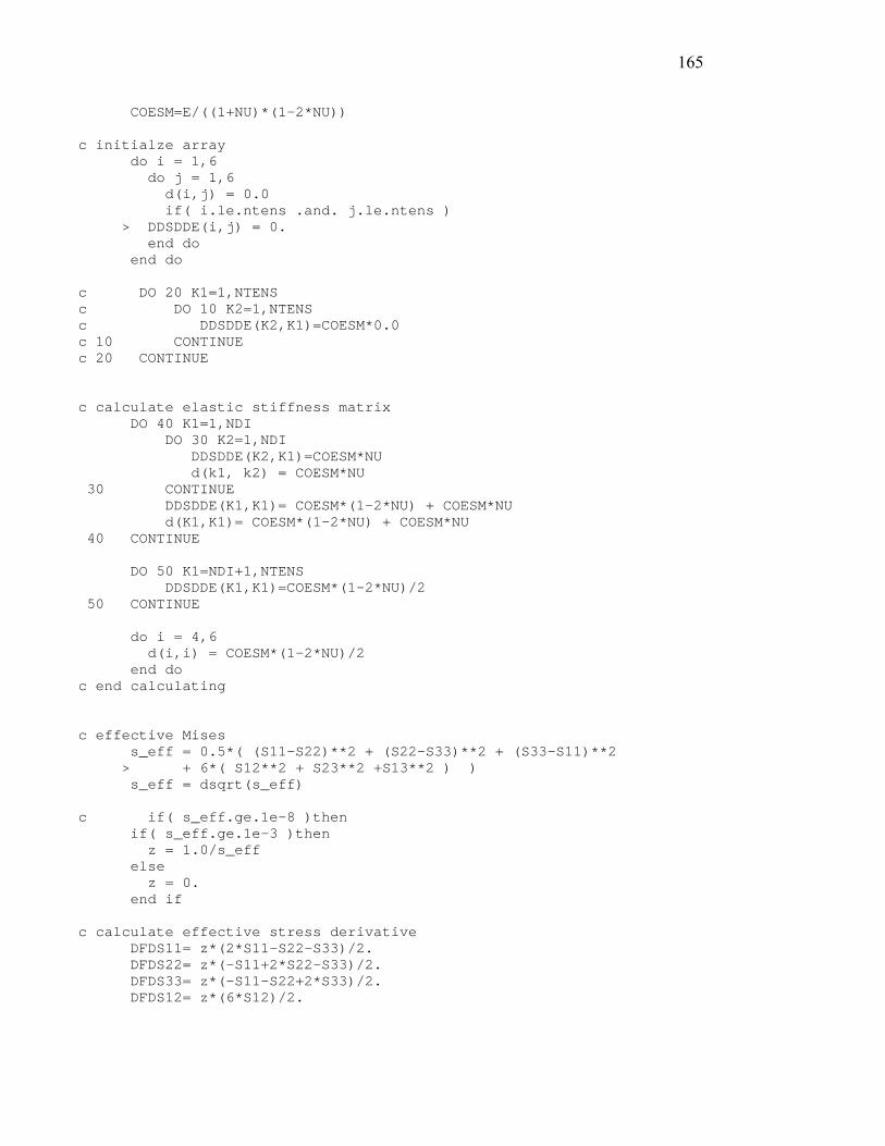
165
COESM=E/((1+NU)*(1-2*NU)) c initialze array do i = 1,6 do j = 1,6 d(i,j) = 0.0 if( i.le.ntens .and. j.le.ntens ) > DDSDDE(i,j) = 0. end do end do c DO 20 K1=1,NTENS c DO 10 K2=1,NTENS c DDSDDE(K2,K1)=COESM*0.0 c 10 CONTINUE c 20 CONTINUE c calculate elastic stiffness matrix DO 40 K1=1,NDI DO 30 K2=1,NDI DDSDDE(K2,K1)=COESM*NU d(k1, k2) = COESM*NU 30 CONTINUE DDSDDE(K1,K1)= COESM*(1-2*NU) + COESM*NU d(K1,K1)= COESM*(1-2*NU) + COESM*NU 40 CONTINUE DO 50 K1=NDI+1,NTENS DDSDDE(K1,K1)=COESM*(1-2*NU)/2 50 CONTINUE do i = 4,6 d(i,i) = COESM*(1-2*NU)/2 end do c end calculating c effective Mises s_eff = 0.5*( (S11-S22)**2 + (S22-S33)**2 + (S33-S11)**2 > + 6*( S12**2 + S23**2 +S13**2 ) ) s_eff = dsqrt(s_eff) c if( s_eff.ge.1e-8 )then if( s_eff.ge.1e-3 )then z = 1.0/s_eff else z = 0. end if c calculate effective stress derivative DFDS11= z*(2*S11-S22-S33)/2. DFDS22= z*(-S11+2*S22-S33)/2. DFDS33= z*(-S11-S22+2*S33)/2. DFDS12= z*(6*S12)/2.
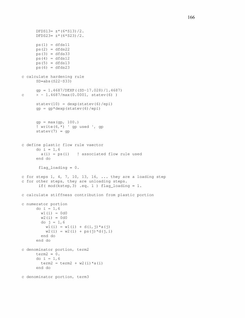
166
DFDS13= z*(6*S13)/2. DFDS23= z*(6*S23)/2. ps(1) = dfds11 ps(2) = dfds22 ps(3) = dfds33 ps(4) = dfds12 ps(5) = dfds13 ps(6) = dfds23 c calculate hardening rule SD=abs(S22-S33) gp = 1.4687/DEXP((SD-17.028)/1.4687) c > - 1.4687/max(0.0001, statev(6) ) statev(10) = dexp(statev(6)/epi) gp = gp*dexp(statev(6)/epi) gp = max(gp, 100.) ! write(6,*) ' gp used ', gp statev(7) = gp c define plastic flow rule vaector do i = 1,6 a(i) = ps(i) ! associated flow rule used end do flag_loading = 0. c for steps 1, 4, 7, 10, 13, 16, ... they are a loading step c for other steps, they are unloading steps. if( mod(kstep,3) .eq. 1 ) flag_loading = 1. c calculate stiffness contribution from plastic portion c numerator portion do i = 1,6 w1(i) = 0d0 w2(i) = 0d0 do j = 1,6 w1(i) = w1(i) + d(i,j)*a(j) w2(i) = w2(i) + ps(j)*d(j,i) end do end do c denominator portion, term2 term2 = 0. do i = 1,6 term2 = term2 + w2(i)*a(i) end do c denominator portion, term3

167
term3 = 0. do i = 1,6 term3 = term3 + gp*s(i)*a(i) end do c calculate plastic stiffness daj do i = 1,6 do j = 1,6 daj(i,j) = 0d0 if( abs(term2+term3).gt.1e-6 ) > daj(i,j) = w1(i)*w2(j)/(term2+term3) end do end do c incremental equivalent plastic strain -- dpe dpe = 0. if( abs(term2+term3).gt.1e-6 )then do i = 1,ntens dpe = dpe + w2(i)*dstran(i)/(term2+term3) end do end if c statev(6) = statev(6) + dpe*s_eff c during unloading, this dpe is 0 if( flag_loading.eq.0 )then dpe = 0. end if c total equivalent plastic strain -- statev(5), SDV5 dpe = max(0d0, dpe) statev(5) = statev(5) + dpe statev(6) = statev(6) + dpe*s_eff c vertical plastic strain -- statev(2), SDV2 statev(1) = statev(1) + a(1)*dpe ! SDV1 statev(2) = statev(2) + a(2)*dpe ! SDV2 statev(3) = statev(3) + a(3)*dpe ! SDV3 statev(4) = statev(4) + a(4)*dpe ! SDV4 c C c TERM2= (DFDS11*NU+DFDS22*(1-NU)+DFDS33*NU)*COESM c c TERM2= (DFDS11*(1-NU)+DFDS22*NU+DFDS33*NU)*COESM c C c C SD=DEVIATOR STRESS c C c SD=abs(S22-S33) c TERM3a = 1.4687/EXP((SD-17.028)/1.4687) c term3a = 100000. c term3 = term3a * S22 c C c C DTERM23=DIFFERNECE between TERM2 AND TERM3 c C

168
do k1 = 1,ntens if( DDSDDE(K1,K1) .lt. daj(k1,k1) )then write(6,*) 'ERR: unexpected negative ', k1 > ,DDSDDE(K1,K1), daj(k1,k1) write(6,'(a,6(1pe11.4,2h, ))') ' stres -> ',stress write(6,'(a,6(1pe11.4,2h, ))') ' ps ', ps write(6,'(a,6(1pe11.4,2h, ))') 'gp,|s22|,Ep ', gp, abs(s22), Ep write(6,'(a,6(1pe11.4,2h, ))') > ' t2, t3, sdv1 ',term2,term3,statev(1) write(6,*) ' -- d -- ' write(6,'(6(1pe11.4,2h, ))') d write(6,*) ' -- daj -- ' do i = 1, ntens write(6,'(6(1pe11.4,2h, ))') (daj(i,j),j=1,ntens) end do call xit() end if end do c c form final elastic-plastic stiffness for loading situation w = 1. if( dpe.lt.1e-8 ) w=0. DO K1=1,NTENS DO K2=1,NTENS DDSDDE(K1,K2) = DDSDDE(K1,K2) - > w*daj(k1,k2)*flag_loading end do end do c calculate update stress (forward method is used) DO 71 K1=1,NTENS DO 61 K2=1,NTENS STRESS(K1) = STRESS(K1) + DDSDDE(K1,K2)*DSTRAN(K2) 61 CONTINUE 71 CONTINUE return end
169
Main Difference between AASHTO T274-82, T294-94 (SHRP Protocol P46), and
T307-99
There have been two JTRP research projects prior to the present study in INDOT. One
was done according to the T274-82 and the other was performed following the T294-94.
The current standard procedure for resilient modulus testing is explained in the T307-99.
As seen in Tables A-1 to A-6, the main differences between those procedures are the
combinations of confining and deviator stresses in the procedure of the MR testing. It is
noted that the T274-82 and T294-94 for granular subgrade are composed of very high
deviator stresses. This higher deviator stresses were modified not to overstress the
samples in the T307-99. It is also noted that the T307-99 calls for one procedure for both
cohesive and granular subgrades. Major differences are compared as shown in Table A-1.
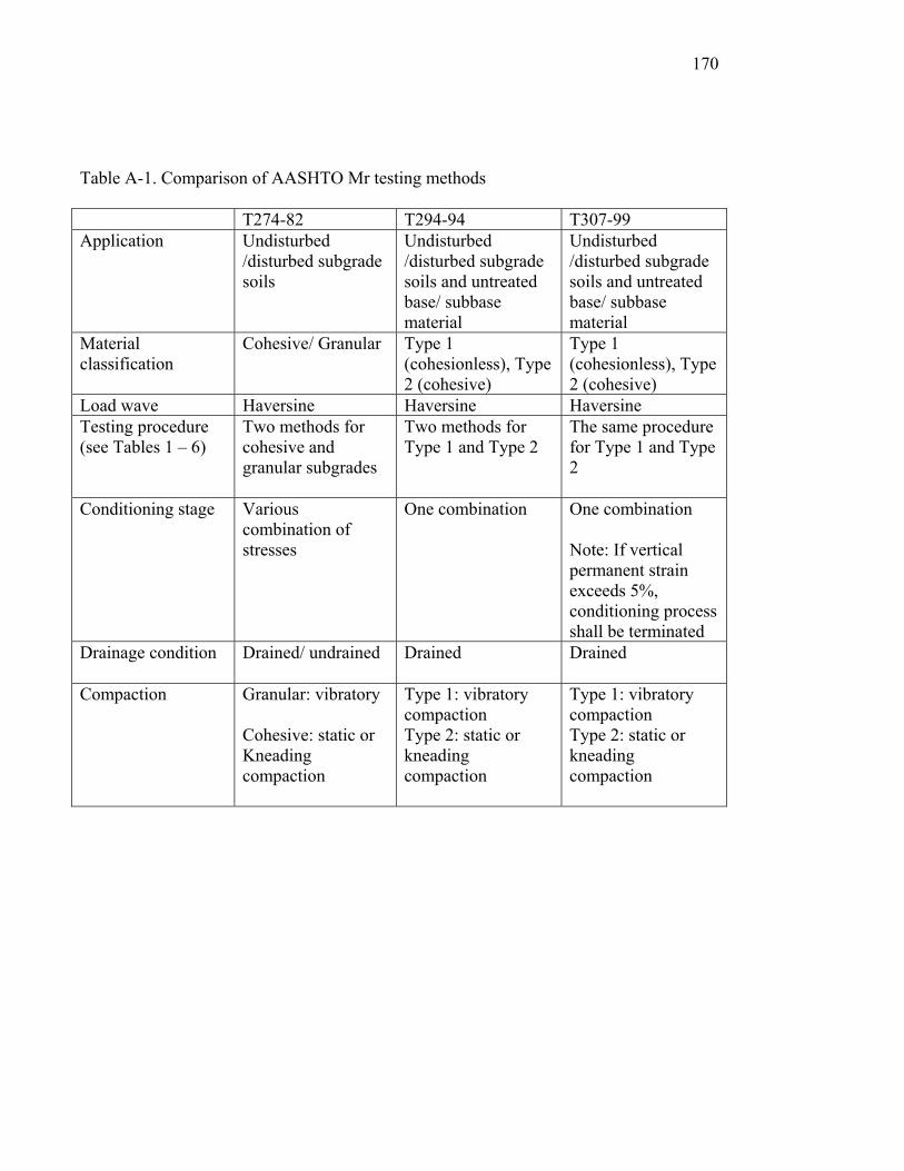
170
Table A-1. Comparison of AASHTO Mr testing methods T274-82 T294-94 T307-99 Application Undisturbed
/disturbed subgrade soils
Undisturbed /disturbed subgrade soils and untreated base/ subbase material
Undisturbed /disturbed subgrade soils and untreated base/ subbase material
Material classification
Cohesive/ Granular Type 1 (cohesionless), Type 2 (cohesive)
Type 1 (cohesionless), Type 2 (cohesive)
Load wave Haversine Haversine Haversine Testing procedure (see Tables 1 – 6)
Two methods for cohesive and granular subgrades
Two methods for Type 1 and Type 2
The same procedure for Type 1 and Type 2
Conditioning stage Various combination of stresses
One combination One combination Note: If vertical permanent strain exceeds 5%, conditioning process shall be terminated
Drainage condition Drained/ undrained Drained Drained
Compaction Granular: vibratory Cohesive: static or Kneading compaction
Type 1: vibratory compaction Type 2: static or kneading compaction
Type 1: vibratory compaction Type 2: static or kneading compaction
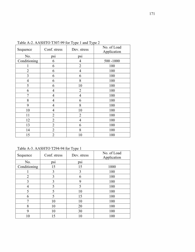
171
Table A-2. AASHTO T307-99 for Type 1 and Type 2
Sequence Conf. stress Dev. stress No. of Load Application
No. psi psi Conditioning 6 4 500 -1000
1 6 2 100 2 6 4 100 3 6 6 100 4 6 8 100 5 6 10 100 6 4 2 100 7 4 4 100 8 4 6 100 9 4 8 100 10 4 10 100 11 2 2 100 12 2 4 100 13 2 6 100 14 2 8 100 15 2 10 100
Table A-3. AASHTO T294-94 for Type 1
Sequence Conf. stress Dev. stress No. of Load Application
No. psi psi Conditioning 15 15 1000
1 3 3 100 2 3 6 100 3 3 9 100 4 5 5 100 5 5 10 100 6 5 15 100 7 10 10 100 8 10 20 100 9 10 30 100 10 15 10 100
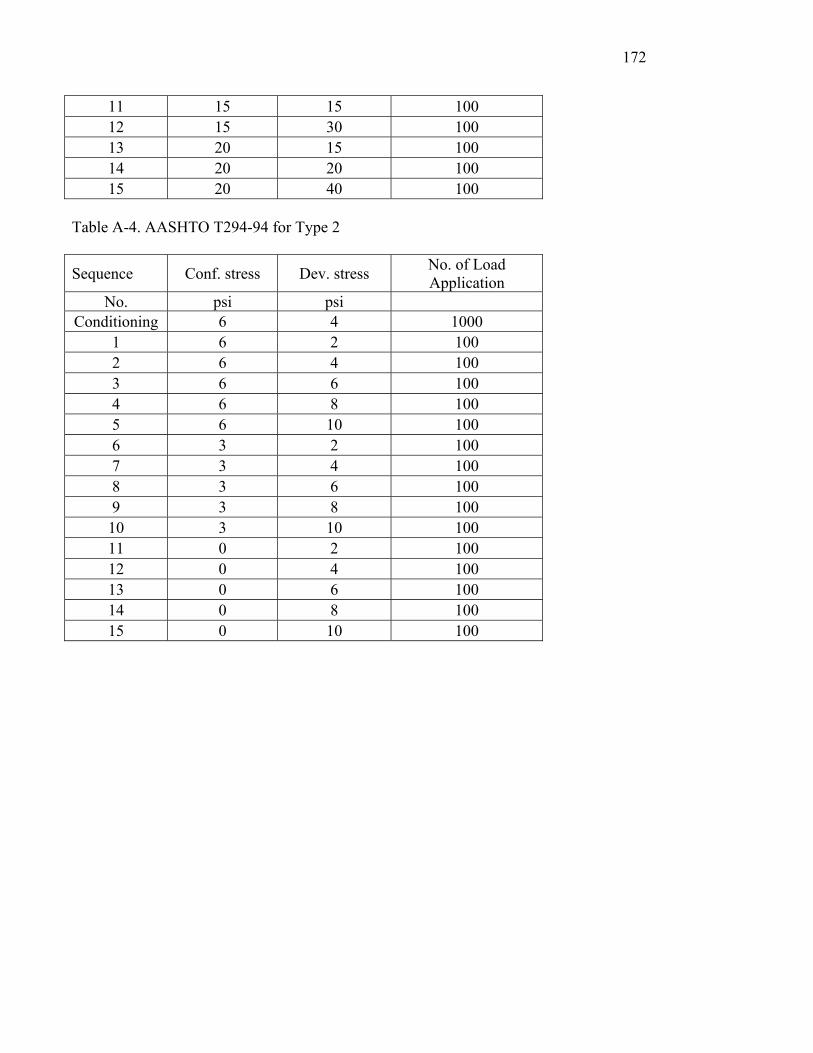
172
11 15 15 100 12 15 30 100 13 20 15 100 14 20 20 100 15 20 40 100
Table A-4. AASHTO T294-94 for Type 2
Sequence Conf. stress Dev. stress No. of Load Application
No. psi psi Conditioning 6 4 1000
1 6 2 100 2 6 4 100 3 6 6 100 4 6 8 100 5 6 10 100 6 3 2 100 7 3 4 100 8 3 6 100 9 3 8 100 10 3 10 100 11 0 2 100 12 0 4 100 13 0 6 100 14 0 8 100 15 0 10 100
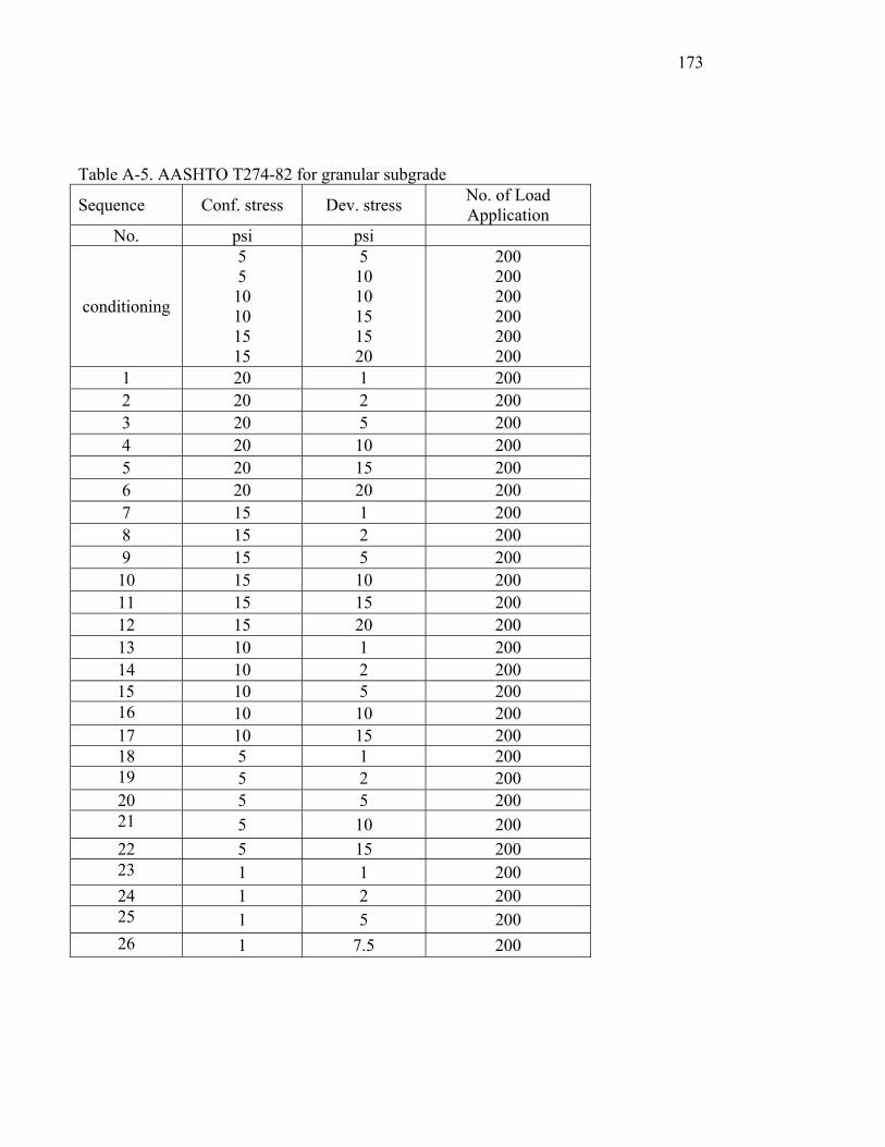
173
Table A-5. AASHTO T274-82 for granular subgrade
Sequence Conf. stress Dev. stress No. of Load Application
No. psi psi
conditioning
5 5 10 10 15 15
5 10 10 15 15 20
200 200 200 200 200 200
1 20 1 200 2 20 2 200 3 20 5 200 4 20 10 200 5 20 15 200 6 20 20 200 7 15 1 200 8 15 2 200 9 15 5 200 10 15 10 200 11 15 15 200 12 15 20 200 13 10 1 200 14 10 2 200
15 10 5 200 16 10 10 200 17 10 15 200 18 5 1 200 19 5 2 200 20 5 5 200 21 5 10 200 22 5 15 200 23 1 1 200 24 1 2 200 25 1 5 200 26 1 7.5 200

174
Table A-6. AASHTO T274-82 for cohesive subgrade
Sequence Conf. stress Dev. stress No. of Load Application
No. psi psi
conditioning
6 6 6 6
6
1 2 4 8 10
200 200 200 200 200
1 6 1 200 2 3 1 200 3 0 1 200 4 6 2 200 5 3 2 200 6 0 2 200 7 0 4 200 8 0 8 200 9 0 10 200

Table A-7. Sites of Subgrade Soils for Resilient Modulus Tests
Soil Soil Collection City County AASHTO USCS Soil Description I65-146 I65 Exit 146 Boone A-4 CL-ML Dark gray silty clay I65-158 I65 Exit 158 Jefferson Boone A-4 CL-ML Dark gray silty clay I65-172
I65 Exit 172 Lafayette Tippecanoe A-6 CL
Dark gray silty clay Dsoil West Lafayette Tippecanoe A-4 CL-ML Dark gray silty clay #1soil 8392L SP.GR A-7-6 CH Dark gray silty clay #2soil 8392L SP.GR A-6 CL Dark gray silt with trace fine sand #3soil 8392L SP.GR A-6 CL Dark gray silt with some fine sand #4soil 8392L SP.GR T-99 A-7-6 CL Dark gray silty clay SR19 587+50; 5m Lt, 8392L SP.GR A-6 CL Dark gray US41
192+65; 80' Rt,SP.GR Gibson A-4 CL
Dark gray Bloomington Bloomington Subdistrict Bloomington Monroe A-7-6 CL red orange clay Orchard West Lafayette Tippecanoe A-6 CL Dark gray clay Test road West Lafayette Tippecanoe A-4 CL Dark gray clay SR 165 2.2E of Poseyville Posey A-4 CL bright gray with many roots US 50 Davies A-3 SP Dark sand Indiana Dunes
SR 49 (N Dune sand) Porter Co. State Park
A-3 SP
Bright sand N Dune SR 49 (N Dune sand) Porter Co.
State Park A-3 SP
Bright sand Wildcat A-1-b SP Dark sand and gravel SR 26 Tippecanoe A-1-b GP
Dark sand and gravel
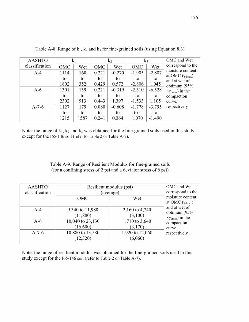
176
Table A-8. Range of k1, k2 and k3 for fine-grained soils (using Equation 8.3)
k1 k2 k3 AASHTO classification OMC Wet OMC Wet OMC Wet
A-4 1114 to
1802
160 to
352
0.221 to
0.429
-0.270 to
0.572
-1.905 to
-2.806
-2.807 to
1.045 A-6 1301
to 2302
159 to
913
0.221 to
0.443
-0.319 to
1.397
-2.310 to
-1.533
-6.528 to
1.105 A-7-6 1127
to 1215
179 to
1587
0.080to
0.241
-0.608 to
0.364
-1.778 to -
1.070
-3.795 to
-1.490
OMC and Wet correspond to the moisture content at OMC (γdmax) and at wet of optimum (95% ×γdmax) in the compaction curve, respectively
Note: the range of k1, k2 and k3 was obtained for the fine-grained soils used in this study except for the I65-146 soil (refer to Table 2 or Table A-7).
Table A-9. Range of Resilient Modulus for fine-grained soils (for a confining stress of 2 psi and a deviator stress of 6 psi)
Resilient modulus (psi) (average)
AASHTO classification
OMC
Wet
A-4 9,340 to 11,980 (11,880)
2,160 to 4,740 (3,100)
A-6 10,040 to 23,130 (16,600)
1,710 to 3,640 (3,170)
A-7-6 10,880 to 13,580 (12,320)
1,920 to 12,060 (6,060)
OMC and Wet correspond to the moisture content at OMC (γdmax) and at wet of optimum (95% ×γdmax) in the compaction curve, respectively
Note: the range of resilient modulus was obtained for the fine-grained soils used in this study except for the I65-146 soil (refer to Table 2 or Table A-7).