simplified estimation of seismic risk for reinforced...
TRANSCRIPT

Submitted to Bulletin of Earthquake Engineering
SIMPLIFIED ESTIMATION OF SEISMIC RISK FOR REINFORCED
CONCRETE BUILDINGS WITH CONSIDERATION OF CORROSION
OVER TIME*
Daniel Celarec
1, Dimitrios Vamvatsikos
2 and Matjaz Dolsek
1
1University of Ljubljana, Slovenia
2University of Cyprus, Cyprus
Abstract. Throughout the world, buildings are reaching the end of their design life and develop
new pathologies that decrease their structural capacity. Usually the ageing process is neglected
in seismic design or seismic risk assessment but may become important for older structures,
especially, if they are intended to be in service even after they exceed their design life. Thus, a
simplified methodology for seismic performance evaluation with consideration of capacity
degradation over time is presented, based on an extension of the SAC/FEMA probabilistic
framework for estimating mean annual frequencies of limit state exceedance. This is applied to
an example of an older three-storey asymmetric reinforced concrete building, in which
corrosion has just started to propagate. The seismic performance of the structure is assessed at
several successive times and the instantaneous and overall seismic risk is estimated for the near
collapse limit state. The structural capacity in terms of the maximum base shear and the
maximum roof displacement is shown to decrease over time. Consequently, the time-averaged
mean annual frequency of violating the near-collapse limit state increases for the corroded
building by about 10% in comparison to the typical case where corrosion is neglected.
However, it can be magnified by almost 40% if the near-collapse limit state is related to a
brittle shear failure, since corrosion significantly affects transverse reinforcement, raising
important questions on the seismic safety of the existing building stock.
Keywords: seismic risk, capacity degradation, corrosion, reinforced concrete frame,
performance-based earthquake engineering, static pushover.
1 INTRODUCTION
Structures are exposed to aggressive environmental conditions which may cause different
types of structural damage. For example, wind, waves, corrosive environment, extreme
temperatures and earthquakes are the influences that can impact many existing structures
every day. Such environmental conditions can cause corrosion or material fatigue that may
lead to the extensive deterioration of mechanical properties of structural elements.
Consequently, the structural capacity degrades over time and considerable costs have to be
incurred just to maintain the serviceability of a structure and to assure its resistance to the
loads that it was designed for.
Driven by the frequent failures of bridge structures, the influence of corrosion on their traffic
load capacity has been widely researched. There, the effects of ageing are more severe since
the entire structure is exposed to the environment. Different studies (Val et al. 1998;
Estes and Frangopol 2001) show that deterioration of capacity resulting from reinforcement
corrosion could have a significant effect on both serviceability and ultimate limit state of
*This article is based on short paper presented at the COMPDYN 2009 Conference (Rhodes, Greece).

2
bridge structures, and thus, have to be properly considered in system reliability assessments.
Until recently, most work has focused on the assessment of aseismic bridges, but the latest
studies (Choe at al. 2009; Kumar et al. 2009) demonstrate that the effect of corrosion becomes
even more meaningful if the bridges are subjected to the seismic load. Less has been done for
buildings, especially to quantify their degrading performance under seismic loads (e.g. Berto
at al. 2009). Thus, we propose to investigate the effect of environmental corrosion on the
seismic behaviour of reinforced concrete (RC) buildings in performance-based earthquake
engineering terms. This effort becomes especially significant for older RC structures designed
and constructed in the 1950–1960 era that are nearing the end of their nominal design life.
The fundamental understanding of the effect of weathering on our ageing infrastructure will
help us actually understand the performance of the structures during their entire life, not just
when they are still intact.
The corrosion of reinforcement, which arises from carbonation phenomena and chloride-
induced penetration, is one of the most important sources of deterioration for RC members
(Val and Stewart 2009). The deterioration process related to the corrosion of reinforcement in
general comprises two parts, that is, the corrosion initiation and corrosion propagation. The
corrosion initiation is the process of diffusion and direct ingress of aggressive agents (e.g.
chloride or carbon dioxide) through protective cover and cracks, while the corrosion
propagation, which starts when the concentration of those agents at bar surface exceeds a
threshold level, is related to formation of different damage in structural elements, such as loss
of cross-sectional area of reinforcing steel, reduction of ductility and mechanical properties of
reinforcing, reduction of bond and crack propagation like spalling and delamination of
concrete protective cover caused by extensive corrosion products (Val and Stewart 2009).
Although models that consider all of the above-mentioned phenomena do exist, they can be
cumbersome. For the purposes of our study, several simplifications were made in order to
provide a simple and efficient estimate of the influence of corrosion on the seismic risk of RC
structures. Therefore, a uniform corrosion was adopted along the longitudinal and transverse
reinforcement bars of exposed structural elements, a simple model compared to more accurate
spatial non-homogeneous pitting corrosion (Stewart 2009). The concrete spalling and
reduction of maximum bond stress between concrete and reinforcement (Berto at al. 2009) bar
were not included in the model. In other words, corrosion only influences the diameter of the
steel bar. Also, the evaluation of the time to corrosion initiation, which depends on a large
number of parameters such as the composition of concrete, its porosity and microstructure,
the degree of pore saturation and the exposure conditions (Val and Stewart 2009), was not
considered; we are focusing on an existing structure in which the corrosion process has just
started to propagate. Therefore, the seismic risk was estimated for a time period of 50 years,
starting from the initiation of corrosion in the structure. Such a simplified approach can be
used for estimating the seismic risk in existing structures, which are expected to be in service
well beyond the time that corrosion has set in, as typically happens when they exceed the
lifetime that they were designed for.
Based on these simplifying assumptions, it would be attractive to use a closed-form
expression to evaluate the performance of an ageing structure in terms compatible with
current performance-based earthquake engineering concepts, i.e. in terms of the mean annual
frequency (MAF) of exceeding a given limit state. One candidate is the engineering demand
parameter (EDP) based methodology introduced by Torres and Ruiz (2007) that will be used
for structural reliability evaluation in combination with the simplified seismic performance
assessment method (Fajfar 2000; Dolšek and Fajfar 2007; Dolšek and Fajfar 2008). It is based
on the SAC/FEMA probabilistic framework proposed by Cornell et al. (2002), in addition to
which, the structural capacity is considered to change in time. Similarly, an intensity measure
3
(IM) based formulation is also considered as an alternative (Vamvatsikos and Dolšek, 2009).
Both are able to provide an expected number of limit-state exceedance events and the overall
time-averaged MAF over the period of interest that can be compared to typical acceptable
rates of exceedance, e.g. the ubiquitous 2% or 10% in 50 years.
In the following sections, the proposed methodology is applied to an existing three-storey
asymmetric non-ductile RC frame building. Our aim is to walk the reader through all the steps
of a practical application on a realistic structure, taking shortcuts and making simplifications
where appropriate to derive a basic result that can help us determine whether corrosion is
worth considering when estimating the seismic performance of a given structure. Let us begin
by briefly summarising the probabilistic framework.
2 SUMMARY OF PROBABILISTIC FRAMEWORK
Existing methods for structural performance assessment, such as that proposed by
Cornell et al. (2002), are usually based on the estimation of the mean annual frequency
(MAF) of violating the designated limit states or performance goals, where the resulting
MAFs are assumed to remain constant throughout the design life of the structure. The MAF of
exceedance of predefined limit states during any given time interval is then equal to the
instantaneous MAF at any time. However, this cannot be the case under severe weathering
conditions, where significant capacity degradation is expected to take a place and as a
consequence the MAF increases with time. Thus, additional effort has to be done to account
for capacity degradation over time.
Since the numerical evaluation of the time integral adds another layer of complexity,
simplified methods for structural reliability evaluation considering the capacity degradation
over time have recently been developed. In the present study we primarily use the reliability
framework introduced by Torres and Ruiz (2007). Their method is a straightforward
extension of the probabilistic framework proposed by Cornell et al. (2002), with the added
assumption that the structural capacity C is a random variable with a probability density
function Cf c , which changes with time. Therefore the conditional probability of failure
,P C D y is also a function of time and the expected number of limit state
exceedance events within the time interval 0 0,t t t can be expressed as:
0
0
0 C0 0
( ), ,
t t
t
dH yE t t P C D y f c dy dc d
dy. (1)
The variables of Eq.(1) are explained in more detail elsewhere (Torres and Ruiz 2007). The
analytical solution of Eq. (1) provides two different formulations, which were both used in
our study, that is, the Engineering Demand Parameter (EDP) based formulation and the
Intensity Measure (IM) based formulation, which differentiate on how the seismic demands
(D) and structural capacities (C) are defined. The formulations are explained in more detail in
the following sections.
2.1 The EDP based formulation
The EDP based formulation, proposed by Torres and Ruiz (2007), is based on the engineering
demand parameter, i.e. a measure of the structural response. In that case,Eq. (1) can be
expressed in closed form, similarly as derived by Cornell et al. (2002). The expected number
of limit state exceedance events ηedp over the time interval 0 0,t t t and the average MAF AVG
edp can then be written as:
4
2
edp0 2 2 2 2 AVG
edp 0 g,ls DR CR DU CU 0 edp2ˆ, exp , ,
2
kt t H a t t
b t, (2)
where )(H is the mean seismic hazard function, k0 and k are the parameters of the power-law
approximation to the hazard curve, DR
is the dispersion measure for aleatory randomness in
displacement demand, CR
is the dispersion measure for aleatory randomness in displacement
capacity, DU
and CU
are, respectively, the dispersion measures for epistemic uncertainty in
displacement demand and capacity, and b is the exponent of the approximate power-law
relationship between the IM and EDP. 0
g,lsa is the seismic intensity measure, in our case the
peak ground acceleration, related to the median of the limit state capacity
0C t at the
beginning of the evaluation time interval (t0, t0+Δt), and Ω is a derived parameter covering
the specified time interval:
1
b00
g,ls
ˆˆ
C ta
a (3)
1
0
0
0
, 1 1( )
k
bt b tt t
b k t. (4)
The simplified approach presented above is based on several assumptions. The hazard curve
has to be approximated considering an appropriate interval around 0
g,lsa , and the relationship
between the IM and the EDP has to be fitted around the 0C t , both accomplished by the
following power-law expressions:
-k b
0ˆˆ ˆ ˆ , g g gH a k a D t a a . (5)
Additionally, the median capacity C t is assumed to vary linearly with time:
ˆ , >0 and 0C t t , (6)
where α in β are the parameters defining the linear function (note, that parameter β without
subscripts has no relation with those defining dispersion measures in Eq. (2)). It is also
assumed that all dispersion measures and the parameters of the relationship between the IM
and the EDP (a, b) are constant over the integration time interval Δt. The demand D(t) and
capacity C(t) are assumed to be lognormally distributed. The dispersion measures related to
demand and capacity are therefore defined as the standard deviation of the logarithm of the
demand and capacity, respectively.
2.2 The IM based formulation
Unlike the case of the EDP formulation, the IM based approach (e.g. Cornell et al. 2002)
requires structural capacity expressed in terms of the earthquake intensity measure, which can
be for example, the spectral acceleration Sa or the peak ground acceleration ag. This
alternative formulation has several theoretical advantages compared to the standard EDP-
based formulation. For example, an approximation of the relationship between the seismic
intensity measure and engineering demand parameter is not needed, and the IM based
formulation also does not require any correlation assumptions between demand and capacity.
Starting again from Eq. (1) and using similar assumptions to those presented earlier,
(Vamvatsikos and Dolšek 2009) have derived the expression for the expected number of limit

5
state exceedance events ηedp over the time interval (t0, t0+Δt) and the average MAF AVG
imλ as
follows:
1
02-k
g,ls0 2 2 AVG im
im 0 0 g,ls Rag Uag im0
g,ls
ˆ Δˆ,Δ exp + 1 1 ,
ˆ2 (1 )
k
a ηk γ tη t t k a β β λ
γ k a Δt
(7)
where βRag and βUag are the dispersion measures in intensity measure for randomness and
uncertainty, k0 and k are the parameters of the hazard curve approximation, and 0
g,lsa is the
median peak ground acceleration corresponding to the predefined limit state (e.g. near
collapse limit state). Note that parameters 0
g,lsa
of the Eq. (2) and Eq. (7) are in general
different, since in the first case the 0
g,lsa is determined indirectly through EDP-capacity whereas
in the later case it is determined directly through IM-capacity.
Expression (7) was derived considering the assumption that structural capacity Ĉ(t) varies
linearly in time. For mathematical convenience it was assumed that value of that linear
function at time t0 corresponds to the structural capacity at the same time, which is a further
simplification compared to the Torres and Ruiz (2007) formulation. Thus, the linear function
of structural capacity C t is defined with a single parameter γ only:
0ˆ ˆ , 0,C t C t t (8)
where γ defines the slope of the linear function.
2.3 Simplified method for seismic performance assessment of structures
Determination of the relationship between the seismic intensity measure and the engineering
demand parameter may become extremely time-consuming. This is especially the case if the
structural response is estimated with nonlinear dynamic analysis, which, even for a single
instant in the building’s lifetime, has to be performed for several intensity measures and
different ground motion records, e.g. with incremental dynamic analysis (IDA) (Vamvatsikos
and Cornell 2002), in order to capture randomness due to earthquakes. In addition, analyses
will have to be performed for different times within the lifetime of interest to capture the
effect of corrosion. Therefore, for practical application, simplified analysis methods become
very attractive. In our study, the time-dependent relationship between the seismic intensity
measure and the engineering demand parameter was determined with the incremental N2
analysis (IN2) (Fajfar 2000; Dolšek and Fajfar 2007). It is a simplified nonlinear method for
seismic performance assessment of structures and represents an alternative to IDA
(Vamvatsikos and Cornell 2002).
The procedure for determination of the IN2 curve is explained elsewhere (Dolšek and Fajfar
2007). For common structural systems with moderate or long fundamental period(s) the IN2
curve results in a straight line. In this case the “equal displacement rule” applies, i.e. b=1.0
(Eq. (5)), up to the “failure” point, which is conservatively represented by the near collapse
limit state. After “failure”, the IN2 curve becomes a horizontal line. In more general cases, the
IN2 curve can be approximated in the same way as a mean IDA curve, i.e. from two points of
the actual curve, e.g. from the points representing the damage limitation and near collapse
limit states, or by regression over several discrete points.
Since the IN2 curve is only a “central” (mean or approximately median) result, it does not
contain any dispersion information. Therefore the dispersion values for randomness in
displacement demand βDR and displacement capacity βCR cannot be determined. A possible
alternative is using SPO2IDA instead, a simple-to-use tool that employs complex R-μ-T
relationships to provide the median and the 16, 84 percentiles of demand or capacity

6
(Vamvatsikos and Cornell 2006). This allows the estimation of both the needed median
dispersion of capacity for complex pushover shapes and will provide accurate results.
Alternatively, they can be estimated directly by performing IDA for the equivalent SDOF
system as also shown in Dolšek and Fajfar (2007). Still, our pushover shapes are practically
elasto-plastic, allowing the use of existing results from other works, (e.g. Dolšek and Fajfar
2007; Ruiz-Garzia and Miranda 2003), who have found that the coefficient of variation for
the displacement of such SDOF systems varied from 0.4 for structures with a moderate or
long natural period, to 0.7 for structures with a short predominant period. The determination
of dispersion measures for uncertainty in displacement demand βDU and capacity βCU is in
general possible to determine with the IN2 method, but requires a probabilistic structural
model, i.e. a model with appropriate consideration of parameter uncertainties, which is not
within the scope of this paper. For a simplified approach, it is convenient to predetermine the
dispersion measures for uncertainty. For example, dispersions for steel frames have been
proposed in the FEMA-350 Guidelines (2000). They may serve as rough estimates also for
some other structural systems. For example, the total uncertainty dispersion measure 2 2 0.5
UT DU CU( ) 0.35 was applied for a global inter-story drift evaluation in the case of
low-rise buildings within the SAC/FEMA seismic performance evaluation (Yun et al. 2002).
The dispersions in intensity measure due to randomness and modelling uncertainties for
different types of structural systems and for the IM based approach were recently proposed in
FEMA P695 (2009). The values for record-to-record and modelling-related variability are in
range of 0.35 to 0.45 for randomness and 0.2 to 0.65 for uncertainties.
3 EXAMPLE OF THE THREE-STOREY RC FRAME BUILDING
As an example of our methodology, we will estimate the seismic risk for an existing frame
building, in which the reinforcement corrosion has just initiated. The structure is located in a
region of moderate seismic hazard and high level of reinforcement corrosion risk area, a
typical scenario for most coastal areas in the Mediterranean. The objective of the analysis is to
estimate the increase in seismic risk for two predefined near-collapse limit states as the
associated structural capacity degrades with time.
The structure was analysed at different time instants (t0+Δt), in which t0 relates to the initial
condition of the existing structure, when corrosion attack was detected, and Δt is the time
interval during which the propagation of corrosion is taking place. Since the evaluation
interval is taken to be [0, 50yrs], t0 was set to zero in Eq. (2), (4) and (8). For the discussions
to follow, the term “initial structure” will relate to the structure at time t0, at which it was
assumed that reinforcement corrosion did not affect the structural capacity yet, and the term
“degraded structure” will relate to the structure affected by corrosion at selected time instants
Δt.
3.1 Description of the structure and model
The example structure is a three-storey asymmetric reinforced concrete frame building. This
structure was pseudo-dynamically tested within the European research project SPEAR
(Seismic performance assessment and rehabilitation of existing buildings, M. Fardis and P.
Negro, coordinators) and analysed in previous studies (e.g. Fajfar et al. 2003). The elevation,
the plan of the building and the reinforcement of typical cross sections of the columns and
beams are shown in Figure 1. The structure was designed for gravity loads only.

7
Figure 1: a) The elevation and plan view of example structure, and b) typical cross-sections and reinforcement in
columns and beams.
The columns and beams of the structure were modelled by one-component lumped plasticity
elements, which consist of an elastic beam-column element and two inelastic rotational hinges
at the ends, defined by a moment-rotation relationship. These relationships were determined
for the columns by properly taking into account their axial load and its interaction with the
moment capacity. Gravity loads for this RC structure amounted to 6.3 kN/m2 and 6.2 kN/m
2
for first two stories and top storey, respectively.
Rigid diaphragms were assumed at the floor levels due to monolithic RC slabs. Consequently
the masses were lumped at the mass centres. The lumped masses and the corresponding mass
moments of inertia amounted to 65.5 t and 1196 tm2 for the first two stories, and 64.1 t and
1254 tm2 for the top storey, respectively. The centreline dimensions of the elements were used
with the exception of beams which are connected eccentrically to the column C6. Using
centreline dimensions, the storey heights of 2.75 and 3.0 m, respectively, for the first and
upper two storeys, were assumed.
A schematic moment-rotation relationship is shown in Figure 2. The yield (My) and maximum
moment (Mm) was determined from appropriate section analysis. The characteristic rotations,
which describe the moment-rotation envelope of a plastic hinge, were determined according
to the procedure described by Fajfar et al. (2006). The zero moment point was assumed to be
at the mid-span of the columns and beams. Therefore the rotations θy for moment-rotation
envelopes of columns and beams were calculated using the formula:
y span
y
eff
6
M l
E I, (8)
where lspan is the length of a beam or column, E is the modulus of elasticity and Ieff is the
effective moment of inertia of the element (0.5 I).

8
y
m
nc
Mm
My
Y M: Mm
= Mmax
NC: Mnc
= 0.8 Mm
Mo
men
tRotation
u
Figure 2: Schematic moment-rotation relationship of a plastic hinge in columns and beams.
The near collapse rotation θnc,c in the columns, which corresponds to a 20 % reduction in the
maximum moment, was estimated by means of the Conditional Average Estimator (CAE)
method (Perus et al. 2006), whereas the near collapse rotation for hinges in beams θnc,b were
determined using the formula defined in Eurocode 8 (2005):
ywsx
c d
0.225 0.35
100ν Vnc,b
el
1 max(0.01; '0.016 (0.3 ) 25 (1.25 )
max(0.01; )
f
f
c
Lf
h. (9)
where γel is equal to 1.0 (mean values), parameter ν is the normalised axial load (for beams:
ν=0), ω and ω’ are the mechanical reinforcement ratios of the tension and compression
longitudinal reinforcement, respectively, fcm and fyw are the mean strength of concrete (MPa)
and yield strength of steel (MPa), respectively, ρsx is the ratio of transverse steel parallel to the
direction of loading, ρd is the steel ratio of diagonal reinforcement in each diagonal direction
and α is the confinement effectiveness factor. All beams are defined as members without
detailing for earthquake resistance. Therefore the rotations at near collapse limit state θnc,b are
multiplied by 0.825. The post-capping or negative-stiffness part of moment-rotation envelope
is determined under the assumption that the ratio between the ultimate rotation θu,b and
rotation at maximum moment θm,b is 3.5.
The degradation of capacity over time was modelled only via the simplified model of
corrosion of longitudinal and transverse reinforcement in the external (i.e. exposed) elements
of the structure. In general, the corrosion decreases the diameter of reinforcement and the
bond stress between the concrete and steel bars. The later phenomenon and as well as spalling
of concrete were not considered in this stage of the study. Therefore in our model the
corrosion influences only the diameter of the steel bar. The reduced diameter Drb(t) of a
reinforcing steel bar with initial diameter of Db (mm), which is subjected to corrosion for a
time period (years) Δt=t-t0 (t0 relates to the initial condition of the building and is equal to 0)
is, according to Pantazopolou and Papoulia (2001):
rb b corr0,023 ,D D i t (10)
where icorr represent the mean annual corrosion current per unit anodic surface area of steel
(μA/cm2). In our analysis the corrosion current icorr=1.2 μA/cm
2 was considered, which
corresponds to a high level of reinforcement corrosion (Pantazopolou and Papoulia 2001).
In order to determine the structural capacity as a function of time, six structural models M0,
M10, M20, M30, M40 and M50 were prepared on the OpenSees platform (McKenna and Fenves
2004) in combination with the PBEE toolbox (Dolsek 2009). These correspond to the initial
condition of the building at time t0=0 and to the degraded structure (affected by corrosion)
after 10, 20, 30, 40 and 50 years of corrosion propagation, respectively. The first three modal

9
periods of the initial 3D structure are: T1=0.80 s T2=0.67 s and T3=0.538 s and are changing
with time as the corrosion reduces the capacity. The period T2 and the associated mode shape
actually correspond to the first translational mode in the Y direction, which is the most critical
for the seismic performance of the structure. Therefore the second mode shape will be
exclusively used for applying the N2 method.
3.2 Definition of the limit states and nonlinear static analyses
The MAF of exceedance was determined for a near collapse limit state and for additional
limit state which is related to the potential brittle failure and defined by a storey shear
demand/capacity ratio (DCR) equals 0.5. The reason for such a definition of the second limit
state is described later on in this Section.
According to European standard Eurocode 8 (2005) the near collapse (NC) limit state at the
element level is defined with the ultimate rotation θnc, which corresponds to 20% drop of
moment in the softening range of the moment-rotation relationship (Figure 2), and it is related
to a ductile collapse mechanism. The NC limit state can also be defined on the basis of the
shear strength, which is related to a brittle collapse mechanism. In this case the shear strength
(capacity) of an element was calculated according to Eurocode 8 (2005):
pl
R c c
el
VTOT c c W
1min ;0,55 1 0,05min 5;
2
0,16max 0,5;100 1 0,16min 5; ,
V
h xV N A f
L
Lf A V
h
(11)
where γel was assumed 1.0 in order to get the mean value of the shear strength, h is the depth
of cross-section, x is the height of compressive zone, Lv is the moment-shear ratio (M/V), Ac is
the cross-section area calculated as bw∙d, fc is the concrete compressive strength, ρtot is the
total longitudinal reinforcement ratio and Vw is the contribution of transverse reinforcement to
shear resistance, taken as equal to:
w w w yw ,V b z f (12)
where w is the transverse reinforcement ration, bw is the width of the rectangular web of the
cross-section, z is the length of the internal lever arm and fyw is the yield stress of the
transverse reinforcement.
Since the limit state at the building level is not defined in the European standard it was simply
assumed that the near collapse limit state appears whether the base shear strength of structure,
in relation to its static pushover curve, reduces to 20% of its maximum value, or the storey
shear demand/capacity ratio (DCR) at any storey is equal or exceeds 1. Such definition is
needed since the elastic model of shear was used in the analysis. In this place it is worth to
emphasize that the structure under investigation is not sensitive to a brittle failure (shear DCR
never exceeds 1) although corrosion significantly affects transverse reinforcement. However,
we wanted to show how much the reduction of transverse reinforcement due to corrosion
affects the MAF of violating the potential brittle limit state. Therefore, the MAF was estimated
for an additional limit state (i.e. a potential brittle limit state), which is defined by a storey shear
demand/capacity ratio (DCR) at any storey equals 0.5. Note that this limit state limit state is
not related to near collapse limit state, but is a good indicator of the effect of corrosion on a
potential shear failure.
10
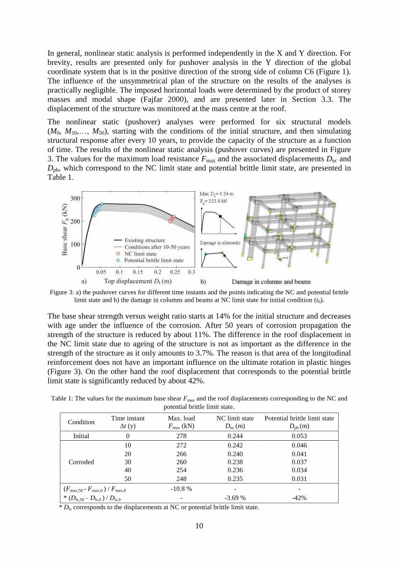
In general, nonlinear static analysis is performed independently in the X and Y direction. For
brevity, results are presented only for pushover analysis in the Y direction of the global
coordinate system that is in the positive direction of the strong side of column C6 (Figure 1).
The influence of the unsymmetrical plan of the structure on the results of the analyses is
practically negligible. The imposed horizontal loads were determined by the product of storey
masses and modal shape (Fajfar 2000), and are presented later in Section 3.3. The
displacement of the structure was monitored at the mass centre at the roof.
The nonlinear static (pushover) analyses were performed for six structural models
(M0, M10,…, M50), starting with the conditions of the initial structure, and then simulating
structural response after every 10 years, to provide the capacity of the structure as a function
of time. The results of the nonlinear static analysis (pushover curves) are presented in Figure
3. The values for the maximum load resistance Fmax and the associated displacements Dnc and
Dpb, which correspond to the NC limit state and potential brittle limit state, are presented in
Table 1.
Figure 3: a) the pushover curves for different time instants and the points indicating the NC and potential brittle
limit state and b) the damage in columns and beams at NC limit state for initial condition (t0).
The base shear strength versus weight ratio starts at 14% for the initial structure and decreases
with age under the influence of the corrosion. After 50 years of corrosion propagation the
strength of the structure is reduced by about 11%. The difference in the roof displacement in
the NC limit state due to ageing of the structure is not as important as the difference in the
strength of the structure as it only amounts to 3.7%. The reason is that area of the longitudinal
reinforcement does not have an important influence on the ultimate rotation in plastic hinges
(Figure 3). On the other hand the roof displacement that corresponds to the potential brittle
limit state is significantly reduced by about 42%.
Table 1: The values for the maximum base shear Fmax and the roof displacements corresponding to the NC and
potential brittle limit state.
Condition Time instant
Δt (y)
Max. load
Fmax (kN)
NC limit state
Dnc (m)
Potential brittle limit state
Dpb (m)
Initial 0 278 0.244 0.053
Corroded
10 272 0.242 0.046
20 266 0.240 0.041
30 260 0.238 0.037
40 254 0.236 0.034
50 248 0.235 0.031
(Fmax,50 - Fmax,0 ) / Fmax,0
* (Dls,50 – Dls,0 ) / Dls,0
-10.8 %
-
-
-3.69 %
-
-42%
* Dls corresponds to the displacements at NC or potential brittle limit state.

11
3.3 Seismic capacity at different time instants
The definition of the structural capacity as a function of time differs depending on the
probabilistic formulation. The EDP based formulation requires the structural capacity
expressed in terms of an appropriate engineering demand parameter, whereas the IM based
formulation depends on the structural capacity being expressed via the intensity measure, e.g.
peak ground acceleration or spectral acceleration.
In the case of the EDP-based formulation, the structural capacity is defined in terms of the
maximum roof displacement that corresponds to the predefined limit states, whereas for the
IM-based formulation, the structural capacity is defined with the lowest peak ground
acceleration that causes violation of each limit state. The relation between the maximum roof
displacement and the peak ground acceleration is computed with the N2 method (Fajfar 2000)
for the seismic load, which is defined with the elastic response spectrum according to
Eurocode 8 (2004) for soil class C (S=1.15, TC=0.6 s).
The roof displacements that correspond to the separate limit states were already reported in
Section 3.2. In this Section determination of peak ground acceleration capacity ag,nc is
explicitly demonstrated only for the NC limit state and for the initial building condition, i.e.
for model M0, while for degraded structures and for the potential brittle limit state only the
final results are presented.
Once the results of pushover analysis are available, the pushover curve has to be idealized as
shown in Figure 4a in order to determine the properties of the equivalent single degree of
freedom (SDOF) model. The results of this idealization are the yield force Fy and yield
displacement Dy. The properties of the SDOF system are then determined by dividing the
corresponding properties of the MDOF system by the transformation factor
2
1.27; 128.6 t,SDOFSDOF i i
i i
mm m
m (2)
where mSDOF is the mass of SDOF system, m={65.6, 65.6, 64.1} t is a vector of storey
masses, and Y={0.28, 0.70, 1.00} is the mode shape vector (normalized by its roof
component) of the predominant translational mode shape in the Y direction, which in our
example corresponds to T2=0.67 s. The yield point of the equivalent SDOF system is obtained
simply as y y 0.025 m d D and y y 220 kN.f F The period of the SDOF system
is calculated as follows:
SDOF y
SDOF
y
2 0.753 sm d
Tf
. (13)
The periods of all equivalent SDOF systems over all building ages are obviously within the
medium-period range of the spectrum (Figure 4) and exceed the characteristic period TC,
which is the corner period between the constant acceleration and constant velocity ranges in
an idealized Newmark-Hall type spectrum. Therefore, the equal displacement rule can be
applied for the determination of the mean (or approximately median) spectral acceleration,
which corresponds to the NC limit state. Therefore the Sae,nc is:
2
2
ae,nc nc
SDOF
213.4 m/sS d
T (14)

12
wherenc nc d D , and the mean/median peak acceleration ag,nc corresponding to the NC
limit state is determined from the elastic spectrum as follows:
ae,nc SDOF 2SDOF
g,nc
C
5.87 m/s 0.598 g2.5
S T Ta
S T. (15)
The above evaluation of the ag,nc can be presented in the acceleration-displacement (AD)
format together with the capacity diagram of the SDOF system (Figure 4b).
Figure 4: a) Idealization of the pushover curve for model M0 and b) the AD format for the equivalent SDOF
system.
This procedure was repeated to evaluate the peak ground acceleration capacity that
corresponds to the NC and potential brittle limit states and for all degraded structures (models
M10 to M50). The resulting peak ground acceleration capacities ag,nc and ag,pb are presented in
Table 2. The reduction in peak ground acceleration capacities for both limit states is similar to
that shown before for the maximum roof displacement (Section 3.2, Table 1) and is about
4.5% for the NC limit state and 40% for the potential brittle limit state.
Table 2: The peak ground acceleration capacities ag,nc and ag,pb for the NC and potential brittle limit states.
Condition Time instant
Δt (y)
NC limit state
ag,nc (g)
Potential brittle limit state
ag,pb (g)
Initial 0 0.598 0.131
Corroded
10
20
30
40
50
0.592
0.586
0.581
0.575
0.571
0.114
0.103
0.093
0.086
0.079
*(ag,ls,50 - ag,ls,0 ) / ag,nc,0 - 4.5 % -40 %
*ag,ls corresponds to the peak ground acceleration capacities for NC or potential brittle
limit state.
The results presented in Table 2 are used as input data for the definition of the seismic
capacity as an approximately linear function of time (Eq. (2) and (7)). The parameters α, β
and γ that approximate the capacity as a linear function were calculated using linear
regression (i.e. the method of least squares) for the EDP and IM-based format. The results are
presented in Table 3. The roof displacements corresponding to each limit state defined at each
time instant are presented in Figure 5. The fitted lines approximate the linear decrease of the
median capacity with time after corrosion initiation.

13
Table 3: The parameters defining the linear functions for structural capacity in time.
Formulation Units NC limit state Potential brittle limit state
EDP-based m, year α=0.244 m, β=-1.86×10⁻⁴
m/y α=0.051 m, β=-4.0×10⁻⁴
m/y
IM-based g, year γ=-5.60×10⁻⁴
g/y γ=-1.1×10⁻³
g/y
Figure 5: The values of maximum roof displacement and peak ground accelerations capacities (ag,ls) at
predefined building ages and their linear approximation for the NC and potential brittle limit state. The results
are presented for a) EDP- and b) IM-based format, respectively.
3.4 Instantaneous and overall seismic risk
The expected number of exceedance events and average MAFs of the NC and potential brittle
limit state were calculated by means of Eq. (2) and Eq. (7) for the initial conditions at time
t0=0, which corresponds to initial structure, and for different time periods, i.e. 10, 20, 30, 40
and 50 years.
The moderate seismic hazard typical for the South-East part of Slovenia (Dolšek and Fajfar
2008), was adopted in the procedure for the estimation of the seismic risk. This was
approximated by a two-parameter seismic hazard function, derived separately for both limit
states. The associated parameters k and k0 were determined by locally fitting the hazard curve
with the function H(ag)=k0∙(ag)-k
(Cornell et al. 2002). The fitting was performed over the
interval from 0.25 ag,ls(t0) to 1,25 ag,ls(t50) (Dolšek and Fajfar 2008), where ag,ls(t0) is the
median peak ground acceleration capacity of the initial structure for the selected limit state,
and ag,ls(t50) is the corresponding capacity of the degraded structure after 50 years, that is, at
the end of the considered time interval. Since ag,ls(t) differs for the NC and the potential brittle
limit state, as marked on the curve on Figure 6, the parameters of the hazard curves also differ
for both defined limit state, a fact that helps improve the accuracy of the closed form
approximation in Cornell at al. (2002). The parameters are k=3.50, k0=6.40×10⁻⁶
for the NC
limit state and k=1.36, k0=2.73×10⁻⁴
for the potential brittle limit state.
Note that parameter k need not be used in Eqs. (2) and (7) since the hazard corresponding to
ag,ls(t) can be determined directly from the hazard curve. The seismic hazard curve used for
peak ground acceleration is presented in Figure 6. The intensities for return periods 225, 475
and 2475 years are 0.293g, 0.181g and 0.325g, respectively, and the mean/median peak
ground acceleration capacities derived from IN2 for the initial structure, are 0.530g and
0.121g for the NC and potential brittle limit state. As corrosion propagates, these will
decrease with time.

14
Figure 6: The seismic hazard curve and the median points for when the NC and the potential brittle limit state is
achieved.
The dispersions for randomness in displacement demand and capacity were considered to be
equal to 0.4 and 0.2, respectively, whereas the dispersions for uncertainty were considered to
be the same for both the displacement demand and capacity and equal to 0.25. Unlike the
EDP-based formulation, the IM format requires only the dispersion in intensity measure,
which was assumed to be equal to 0.40 for both randomness and uncertainty.
The values for the expected number of exceedance events of the NC and potential brittle limit
state at different times and the corresponding values of the average MAFs, using both the
EDP and IM formulation, are collected in tables 4 and 5. The results are compared with the
case, in which the degradation of structural capacity was neglected. In the latter case, the
instantaneous MAFs of exceedance are all equal to the initial MAF at time t0, and obviously
equal to the time-average MAF as silently assumed in all typical performance-based
earthquake engineering calculations.
The expected numbers of exceedance events for the potential brittle limit state per time
interval of 50 years, using the EDP and IM based formulation, is estimated at 0.39 and 0.40,
respectively, and it is about 39 and 43 % higher than the case in which the degradation was
not considered. Note that it is assumed that the potential brittle limit state is detected when
storey shear demand/capacity ratio at any storey equals to 0.5. On the other hand, the
corrosion has only slightly influenced the moment capacity of the structural elements. Thus,
the expected number of exceedance events for the NC limit state per time interval of 50 years
is increased by only for 7.1 and 8.8 %, if considering the capacity degradation over time and
amounts to 1.48×10⁻²
and 1.46×10⁻²
, depending on which formulation (EDP or IM) is used.
The results of the EDP-based formulation are also presented in Figure 7. The continuous
curve represents the expected number of exceedance events for both limit states considering
the capacity degradation over time and the dashed line represents the case when the
degradation was neglected. The picture 7a and 7b are related to the NC and the potential
brittle limit state, respectively.

15
Table 4: The expected number of exceedance events ηedp and the average MAFs AVG
edpλ for the NC and potential
brittle limit state using the EDP-based formulation.
Condition Time interval NC limit state Potential brittle limit state
Δ yt 2
edp10η AVG 4
edp10λ 2
edp10η AVG 4
edp10λ
No degradation 50 1.38 2.77 27.9 5.59
Corroded
10
20
30
40
50
0.28
0.57
0.86
1.17
1.48
2.80
2.84
2.88
2.92
2.96
5.91
12.5
20.1
28.7
38.8
5.91
6.27
6.69
7.18
7.77
*( xdeg,50 - xnodeg,50 ) / xnodeg,50 + 7.1 % + 7.1 % + 39 % + 39 %
*x corresponds to η or
Table 5: The expected number of exceedance events ηim and average MAFs AVG
imλ for the NC and potential brittle
limit state using the IM based formulation.
Condition Time interval NC limit state Potential brittle limit state
Δ yt 2
im10η AVG 4
im10λ 2
im10η AVG 4
im10λ
No degradation 50 1.34 2.68 27.8 5.56
Corroded
10
20
30
40
50
0.27
0.55
0.84
1.14
1.46
2.73
2.77
2.82
2.87
2.92
5.90
12.6
20.2
29.3
39.8
5.90
6.30
6.76
7.30
7.97
*( xdeg,50 - xnodeg,50 ) / xnodeg,50 + 8.8 % + 8.8 % + 43 % + 43 %
*x corresponds to η or
Figure 7: The expected number of exceedance events of (a) NC limit state and (b) potential brittle limit state
using the EDP based methodology.
3.5 Discussion of the results
One important outcome of the study is the comparison between the EDP and IM-based
formulations. The difference in the results amounts to 2 % and 10 % for NC and potential
brittle limit state, respectively, and it is practically negligible. Basically, the only sources of
difference are the values of the dispersion measures, which in our case were assumed as
average values of the reported dispersions from the literature. All other parameters (see Eqs.
(2) and (7)) practically do not contribute to the differences in the final results obtained by the
EDP- or IM-based approach, especially, since the equal displacement rule is valid and we
have b=1 in Eq. (5b). This confirms the sound basis of both formulations. Still, we expect
them to differ more when the power law approximation of Eq. (5b) is no longer accurate, or

16
when we approach global dynamic instability where the EDP formulation becomes inaccurate
(see Vamvatsikos and Dolšek (2009) and references therein). Finally, the selection of the
value of the dispersion measure becomes more significant when the value of the hazard curve
slope k is high, for example, for the ductile limit state (k=3.5), something that may cause
different results in the two formulations.
For the potential brittle limit state the corrosion significantly increases the seismic risk since
the corrosion of the shear reinforcement has a relatively greater influence on the shear
capacity. This becomes apparent in the static pushover curves, where, consequently, the roof
displacement that corresponds to that limit state decreases by about 4.0 mm per decade or 2.2
cm in 50 years. This is a relatively large reduction compared to the initial condition, in which
the maximum roof displacement at potential brittle limit state amounts to 5.3 cm. However,
this is not true for the case of the NC limit state, since the corrosion of longitudinal
reinforcement practically does not have any influence on the calculated ultimate rotations in
the plastic hinges. As a result, the maximum roof displacements at the ductile NC limit state
for different instants of time decreases by just a few percents, that is 0.9 cm in 50 years (Table
1).
In addition to the averaged results in Tables 4 and 5, the instantaneous MAFs were calculated
(Cornell at al. 2002), which via the EDP-based formulation can be estimated as
2
2 2 2 2
edp 0 g,ls DR CR DU CU2ˆ ( ) exp ,
2
k kt k a t
b (16)
where the seismic intensity measure g,lsˆ ( )a t is related to the selected limit state capacity at
time t. Such values may be of interest as they represent the MAFs derived by a performance
evaluation (based on current probabilistic frameworks) that takes place at that instant in the
building’s lifetime. Therefore the instantaneous MAFs may heavily influence future
rehabilitation decisions. For example, the MAFs of exceedance of the NC and potential brittle
limit states for the initial structure using the EDP-based formulation are estimated at
0.0276×10⁻²
and 0.559×10⁻²
, respectively. Otherwise, the corresponding instantaneous return
periods are around 3620 and 180 years, respectively. For comparison, the instantaneous return
periods for exceedance of the two limit states after 50 years of corrosion propagation decrease
to 2930 and 75 years, respectively.
4 CONCLUSIONS
A simplified methodology has been presented for estimating the seismic performance of
ageing RC structures. Considering the deterioration of longitudinal and shear reinforcement
due to corrosion, and utilizing simplified analysis techniques within a SAC/FEMA-like
probabilistic framework, we are able to estimate the changing mean annual frequency (MAF)
of limit state exceedance as it worsens with time. Finally, the time-average of the MAF of
limit state exceedance is quantified over a continuous time period, providing us with a
cumulative single measure of the structure’s performance as ageing sets in. Two different
approaches were demonstrated to achieve these estimates, based on the EDP and IM
formulation of the SAC/FEMA probabilistic framework, the latter being suitable for all limit
states, even close to global collapse.
In our case-study of a 3-story non-ductile RC structure, both approaches were shown to
produce similar results, as long as we properly assign the values of dispersion, especially, if
the hazard curve slope k is relatively steep. Thus, corrosion is shown to have moderate
influence on the moment capacity of beams and columns, while their shear capacity was

17
heavily degraded. However, the later issue is not reflected in the average MAF of violating
the NC limit state, since the structure is not sensitive to brittle failure. Therefore, we defined a
potential brittle limit state, which indicates shear capacity degradation, and observed around
40 % increase of the average MAF of exceedance events at which the storey shear
demand/capacity ratio exceeds 50 %. This is a significant increase that simply cannot be
ignored if structures contain shear-critical members, something that tends to be the norm in
older RC buildings.
It is envisaged that further refinement of our corrosion model with inclusion of concrete
spalling and bond degradation will additionally increase the estimated seismic risk of ageing
RC structures. Thus, further verifications of such results are needed in order to better
understand the actual risks faced by our ageing infrastructure and appropriately amend our
design codes.
ACKNOWLEDGEMENTS
The authors wish to acknowledge the support of the Cyprus Research Promotion Agency
under grant CY-SLO/407/04 and of the Slovenian Research Agency under grant BI-CY/09-
09-002.
REFERENCES
Berto L, Vitaliani R, Saetta A, Simioni P (2009) Seismic assessment of existing RC structures
affected by degradation phenomena. Struct Saf 31: 284-297.
CEN (2004) Eurocode 8: Design of structures for earthquake resistance. Part 1: General rules,
seismic actions and rules for buildings, EN 1998-1. European Committee for
Standardisation, Brussels, December 2004.
CEN (2005) Eurocode 8: Design of structures for earthquake resistance. Part 3: Strengthening
and repair of buildings. EN 1998-3, European Committee for Standardisation, Brussels,
March 2005.
Choe D, Gardoni P, Rosowsky D, Haukaas T (2009) Seismic fragility estimates for reinforced
concrete bridges subject to corrosion. Struct Saf 31: 275-283.
Cornell CA, Jalayer F, Hamburger RO, Foutch DA (2002) Probabilistic Basis for 2000 SAC
Federal Emergency Management Agency Steel Moment Frame Guidelines. J Struct Eng
128: 526-533.
Dolsek M (2009) Development of computing environment for the seismic performance
assessment of reinforced concrete frames by using simplified nonlinear models. Bull
Earth Eng (in review).
Dolsek M (2009) Incremental Dynamic Analysis with consideration of modeling
uncertainties. Earthq Eng Struct Dynam 38: 805-825.
Dolšek M, Fajfar P (2008) The effect of masonry infills on the seismic response of a four
storey reinforced concrete frame–a probabilistic assessment. Eng Struct 30:3186-3192.
Dolšek M, Fajfar P (2007) Simplified probabilistic seismic performance assessment of plan-
asymmetric buildings. Earthq Eng Struct Dynam 36:2021–2041.
Estes AC, Frangopol DM (2001) Bridge lifetime system reliability under multiple limit states.
J Bridge Eng 6(6): 523-528.
Fajfar P (2000) A nonlinear analysis method for performance-based seismic design. Earthq
Spec 16(3):573-592.

18
Fajfar P, Dolšek M, Marušić D, Stratan A (2006) Pre- and post-test mathematical modeling of
a plan-asymmetric reinforced concrete frame buildings. Earthq Eng Struct Dynam 35:
1359-1379.
FEMA 350 (2000) Recommended seismic design criteria for new steel moment frame
buildings. SAC Joint Venture, Federal Emergency Management Agency, Washington
(DC).
FEMA P695 (2009) Quantification of Building Seismic Performance. ATC-63 Projest Report
– 90 % Draft, Federal Emergency Management Agency, Washington (DC).
Kumar R, Gardoni P, Sanchez-Silva M (2009) Effect of cumulative seismic damage and
corrosion on the life cycle cost of reifirced concrete bridges. Earthq Eng Struct Dynam
38:887–905.
McKenna F, Fenves GL (2004) Open system for earthquake engineering simulation, Pacific
Earthquake Engineering Research Center, Berkeley, California.
http://opensees.berkeley.edu/
Pantazopoulou SJ, Papoulia KD (2001) Modeling Cover-Cracking due to Reinforcement
Corrosion in RC Structures. J Eng Mech 127(4): 342-351.
Peruš I, Poljanšek K, Fajfar P (2006) Flexural deformation capacity of rectangular RC
columns determined by the CAE method. Earthq Eng Struct Dynam 35: 1453-1470.
Rozman M, Fajfar P (2009) Seismic response of a RC frame building designed according to
old and modern practices. Bull Earthq Eng 7:779-799.
Ruiz-Garcia J, Miranda E (2003) Inelastic displacement ratios for evaluation of existing
structures, Earthq Eng Struct Dynam 32:1237-1258.
Stewart MG (2009) Mechanical behavior of pitting corrosion of flexural and shear
reinforcement and its effect on structural reliability of corroding RC beams. Struct Saf
31:19-30.
Torres MA, Ruiz SE (2007) Structural reliability evaluation considering capacity degradation
over time. Eng Struct 29: 2183-2192.
Val DV, Stewart MG, Melchers RE (1998) Effect of reinforcement corrosion on reliability of
highway bridges. Eng Struct 20: 1010-1019.
Val DV, Stewart MG (2009) Reliability assessment of ageing reinforced concrete structures –
current situation and future challenges. Struct Eng Inter 19(9): 211-219.
Vamvatsikos D, Dolšek M (2009) Equivalent constant rates for performance-based seismic
assessment of ageing structures. Struct Saf (in review).
Vamvatsikos D, Cornell CA (2002) Incremental Dynamic Analysis. Earthq Eng Struct
Dynam 31:491-514.
Vamvatsikos D, Cornell CA (2006) Direct estimation of the seismic demand and capacity of
oscillators with multi-linear static pushovers through Incremental Dynamic Analysis.
Earthq Eng Struct Dynam 35(9): 1097–1117.
Yun S-Y, Hamburger RO, Cornell CA, Foutch DA (2002) Seismic performance evaluation
for steel moment frames. J Struct Eng ASCE 128(4): 534-545.