simplified modal analysis for the plant machinery …

Proceedings of the Forty-First Turbomachinery Symposium September 24-27, 2012, Houston, Texas

SIMPLIFIED MODAL ANALYSIS FOR THE PLANT MACHINERY ENGINEER

José A. Vázquez Machinery Consultant

BRG Machinery Consulting, LLC Wilmington, Delaware, USA

C. Hunter Cloud President

BRG Machinery Consulting, LLC Charlottesville, Virginia, USA

Robert J. Eizember

Consultant DuPont Company

Wilmington, Delaware, USA

Copyright © 2012 by Turbomachinery Laboratory, Texas A&M University

process improvemen

85) and M.S. (1987) degrees in Mec

ABSTRACT

al modal analysis and operating deflection shap

INTRODUCTION

Expressed in simple terms, the goal of experimental modal analysis is to determine a system’s natural frequencies and

José Vázquez is a Machinery Consultant at BRG Machinery Consulting, LLC. He has over 22 years of experience in machinery analysis and troubleshooting. His career started in Venezuela as a faculty member at the Universidad Simón Bolivar where he taught courses in kinematics, machinery dynamics and instrumentation, as well as some independent consulting in machinery

vibration. From 1992 to 2001, he worked as lab engineer and research scientist at the Rotating Machinery and Controls (ROMAC) Laboratories at the University of Virginia, providing technical support to member companies and developing rotordynamics and bearing analysis computer programs. Prior to joining BRG, he worked for 10 years at DuPont as a Mechanical Consultant, primarily solving machinery problems and developing advanced measurement techniques.

Dr. Vázquez received his B.S. (Mechanical Engineering, 1990) and MS (Specialization in Rotating Equipment, 1993) from the Universidad Simón Bolίvar in Venezuela. He received his Ph.D. (Mechanical and Aerospace Eng., 1999) from the University of Virginia. He is a member of ASME.

C. Hunter Cloud is President of BRG Machinery Consulting, LLC, in Charlottesville, Virginia, a company providing a full range of rotating machinery technical services. He began his career with Mobil Research and Development Corporation in Princeton, NJ, as a turbomachinery specialist responsible for application engineering, commissioning, and troubleshooting for

production, refining and chemical facilities. During his 11 years at Mobil, he worked on numerous projects, including several offshore gas injection platforms in Nigeria as well as serving as reliability manager at a large US refinery.

Dr. Cloud received his BS (Mechanical Engineering, 1991) and Ph.D. (Mechanical and Aerospace Engineering, 2007) from the University of Virginia. He is a member of ASME, the Vibration Institute, and the API 684 rotordynamics task force.

Robert J. Eizember is a consultant in the field of Mechanical Engineering with the DuPont Company located in Wilmington, DE. He started his career with DuPont in 1989 as a "Field Engineer", gaining experience in a variety of jobs with responsibilities for mechanical equipment operation, project installation, equipment UPtime and reliability, and maintenance ts. During 15 years as a consultant, he has

worked to identify and resolve operational problems with many different types of equipment used in DuPont's manufacturing processes, or their associated structures. A primary focus has been using engineering measurements and techniques such as modal analysis to properly identify the problems.

Robert received his B.S. (19hanical Engineering from the South Dakota School of

Mines and Technology, where he also served two years as an instructor.

Experimentes (ODS) are powerful tools in vibration analysis and

machinery troubleshooting. However, the machinery plant engineer often doesn’t believe such techniques are available given a lack of advanced measurement equipment. This tutorial presents best practices with simplified experimental modal analysis and ODS techniques that can be used by a plant machinery engineer with the limited vibration analysis equipment usually available at a plant site. Minimum requirements and analyzer settings are discussed for a variety of commonly available measurement equipment. For different machinery problems, common measurement pitfalls and limitations are reviewed and, where appropriate, alternative methods are presented. During the presentation, demonstrations of modal testing measurements will be conducted using a portable generic data acquisition system.


perimental data. These natural frequencies and

purpose of this tutorial, it is assumed that a data collector with an off-route mode and FFT capabilities is

e frequency analyzers whe

mode shapes from exmode shapes are collectively referred to as modal

properties. Operating deflection shapes (ODS) is a complimentary

technique to modal analysis. In ODS, the vibration of multiple points on a structure during operation is assembled in a way to provide a visual description of the vibration shape that the structure adopts during operation.

Both modal analysis and ODS are used extensively to improve FEA models and experimental determination of structural properties. These types of uses require a large array of sophisticated equipment and software.

On the other hand, machinery troubleshooting usually does not require the same level of detail and accuracy to produce acceptable results. However, when available, the same type of sophisticated equipment is used as a matter of convenience as it produces faster and more accurate results with less effort. As a consequence, the use of modal analysis in machinery troubleshooting is usually associated with the requirement to have sophisticated equipment and software.

Most data collectors available at plant sites have an off-route mode, allowing the user to use the data collector as a frequency analyzer for troubleshooting purposes. This functionality can be used to determine basic modal properties, in particular, the measurement of natural frequencies.

Measurement of frequency response functions (FRF) and mode shapes usually require additional equipment. In some cases, approximation to mode shapes can be obtained with a basic frequency analyzer as well; a capability that will be highlighted here along with the necessary settings.

This tutorial is organized as a series of recipes and guides for different measurements tasks. Each task is developed as an independent unit discussing the minimum equipment necessary, assumptions, limitations of the results and possible pitfalls. Particular applications are highlighted, providing specific details. Background and instructional material is located in the appendices.

EQUIPMENT CONFIGURATIONS

For the

available. Most data collectors becomn setup in off-route mode and will be referred as such in

this tutorial. Beyond basic frequency analysis, most analyzers have different options regarding the number of channels and FRF calculation capabilities. In addition to the capabilities of the analyzer itself, the type and number of sensors available also limits the measurements.

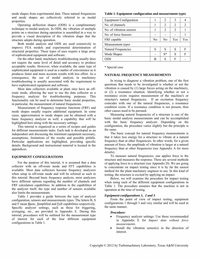
Table 1 provides a guide between the type of analyzer configuration, sensors and measurements types. The letters B, S and F mean Basic, Simplified and Full capabilities respectively. Specific analyzer settings, such as those for triggering, averaging, etc., are provided in Appendix E. During this tutorial, procedures will be outlined for the measurement type of interest for each of the four different equipment configurations in Table 1.

Table 1. Equipment configuration and measurement types

Equ ment Configuration 1 2 3 4 ipNo. of channels 1 2 2 2 No. of vibration sensors 1 2 2 1 No. of force Sensors - - - 1 FRF capable No N Yes Y o esMeasurement types Natural Frequencies S S S F Mode Shapes - S* S F ODS B S F - * Special case

NATURAL FREQUENCY MEASU ENTS

diagnose a vibration problem, one of the first needs to be investigated is whether or not the

machinery, r or not a

reso

es slightly but the principle is the

e, the amplitude of vibration is larger at a natural freq

trate on impact testing since it is by far the easiest met

ents. • Install the vibration sensor(s) in the direction of

interest.

REM

In trying toquestions that vibration is caused by (1) large forces acting on theor (2) a resonance situation. Identifying whethe

nance exists requires measurement of the machine's or structure's natural frequencies. If an excitation frequency coincides with one of the natural frequencies, a resonance condition exists. If a resonance condition is not present, then other causes need to be pursued.

Measuring natural frequencies of a structure is one of the basic modal analysis measurements and can be accomplished with the basic frequency analyzer. Depending on the configuration, the procedure vari

same. The basic concept for natural frequency measurements is

that it takes less energy for a structure to vibrate at a natural frequency than at other frequencies. In other words, for a given amount of forc

uency than at other frequencies (see Appendix A for more details).

To measure natural frequencies, one applies force to the structure and measures the response. There are several methods of applying force to a structure (see Appendix D). We are going to concen

hod for the plant machinery engineer to use. In this kind of testing, the structure is excited by applying an impact.

Below, we will examine the procedure for impact testing when using each of the different equipment configurations in Table 1. The procedure assumes that the machine is not in operation at the time of testing.

Equipment configurations 1, 2 and 3 From the point of view of impact testing, equipment

configurations 1 through 3 and very similar and will be used in the same manner.

Procedure: • Frequency analyzer settings: Use those recommended

in Appendix E for Impact data without force measurem


he structure perpendicularly to the surface, in

e type of wood. A 4x4 (3.5” by 3.5”)

a gentle, sharp tap. A large amount of force

over-ranged, try

g

Figure 1. Response of a damped structure to impact.

• Repeat the impact until the peak hold averaged spectrum does not change any more.

• Stop the acquisition. • The peaks in the spectrum correspond to the damp d

additional frequencies from other sources (Figure 2).

tural frequencies ause the sensor was at a node

both tests are done at once.

Figure 2. Peak hold average of frequency data showing the measured natural frequencies of the structure.

Potential pitfalls and accuracy issues As described previously, the procedure is fairly

straightforward but there are a few points to consider: • The damped natural frequencies measured with this

procedure are approximate. The measured frequency h a

l actual frequency can be anywhere within ∆ /2

olution, the number

ll show excitation frequencies from

the spectrum. The additional peak

th force

• Impact tthe direction of the sensor. For medium size structures a rubber mallet is sufficient, for larger structures use a block of a densblock of oak 3 feet long works well. The impact should beis not required. Keep in mind that a 3 lb rubber mallet can impart up to 5,000 lb of force.

• For the first impact, check the response time window display. This might be difficult to do if your analyzer does not have a trigger function. The response should have gentle decay, as shown in Figure 1. If the response waveform is clipped (flat) at the top and/or bottom, the analyzer input is increasing the input range. If that does not work, replace the sensor with one with lower sensitivity or the amount of force needs to be reduced. In case of sensor overloads (Appendix C), switch to a sensor with lower sensitivity or reduce the amount of force.

• Once the right level of force has been found, switch to the frequency window display and reset the averaging.

• Impact the structure again perpendicularly to the surface, in the direction of the sensor. If you are using triggered collection, wait until the analyzer is ready to acquire the data. If the analyzer is in direct triggerinmode (no trigger), wait long enough between impacts to allow a full set of data to be collected.

enatural frequencies of the structure plus

• Repeat the measurements with the vibration sensor at a different location to make sure that nawere not missed becpoint (Appendix A). If using equipment configuration 2 or 3 with dual sensor capabilities, the second sensor can be installed at a different location and

spectrum is made of discrete frequencies witimited resolution of ∆ , meaning that the

(Appendix B). To increase the resof lines needs to be increased or the frequency range reduced.

• Other excitation sources, such as from other equipment running in the area, may produce peaks in the spectrum. These peaks are not natural frequencies and should not be confused as such. One way to test for these extraneous frequencies is to run the analyzer in free mode (no trigger) and collect data for a while without impacting the structure. The peaks in the spectrum wiexternal sources.

• This procedure is not appropriate for measuring damping. The type of windowing used in this procedure is subjected to leakage and can lead to erroneous interpretations. See Appendix B for details on windowing and leakage.

• If the impacts are repeated at an interval that is shorter than the acquisition time of the analyzer, an additional peak appears in corresponds to the frequency of the impacts.

Equipment configuration 4 The addition of a force sensor and FRF measurements

capabilities adds a level of refinement to the measurements. It also simplifies the interpretation of the results.

Procedure: • Frequency analyzer settings: Use those recommended

in Appendix E for Impact data wimeasurements.

• Install the vibration sensors in the direction of interest. • After selecting an instrumented hammer and tip

suitable for the application (see Appendix D for


). Impact the structure perpendicularly to the

Figure 3. Impact signal, showing a single sharp impact.

• After the first impact, check the time windows. The force should show a single sharp peak as shown on Figure 3. If it shows more than one impact, try again. If you have problems getting a single impact, the hammer is too heavy and a smaller one should b

peak, as shown in the insert in Figure 3, is normal.

to a

the frequency range of interest (see

e energy of the

llection creates noise in the

ages is

is an indicator about the quality of the

0.90 or larger like that shown in Figure 5.

r the impacts

frequency can

guidancesurface, in the direction of the sensor.

Figure 4. Frequency spectrum of the impact signal in Figure 3.

e chosen. The small ringing at the edges of the impact

This is caused by the analyzer’s anti-alias filter. • The response should have gentle decay similar to that

shown in Figure 1. If the response waveform is clipped (flat) at the top and/or bottom, the analyzer input is over-ranged, try increasing the input range. If that does not work, replace the sensor with one with lower sensitivity or the amount of force needs to be reduced. In case of sensor overloads, switchsensor with lower sensitivity or reduce the amount of force.

• The response should fully decay at the end of the window like that shown in Figure 1. If the response has not fully decayed, either increase the number of lines or reduce the frequency range.

• Make sure that the impact has enough bandwidth to excite Appendix D). Ideally, the frequency spectrum should show the amplitude diminishing toward the end of the frequency range as shown in see Figure 4. If the hammer tip is too hard, part of thimpact is used outside the frequency range where it is not needed. If there are any lightly damped natural frequencies beyond the frequency range of the measurements, they can get excited and overload the sensors. This is a particularly annoying occurrence because the sensors overload without any clear indication of the cause. On the other hand, if the tip is too soft, the bandwidth of the excitation is reduced and some of the frequency range of the measurement is wasted and coherence (a measure of the FRF’s quality) will be low in that range.

• Once the right level of force has been found, switch to the frequency window and reset the averaging.

• Impact the structure again, perpendicularly to the surface, in the direction of the sensor. Wait until the analyzer is ready to acquire data. More than one impact during the data comeasurements.

• Repeat the impacts until the number of avercomplete.

• Examine the coherence window. The coherence function varies from 0 to 1. It measures how well the output is related to the input (McConnell, 1995, Ewins, 1984). Itdata. Good quality measurements should have a coherence of To improve the coherence for a particular frequency range of interest, increase the number of averages. If that does not help, reduce the input range for the particular sensor. In some cases, it may be necessary to use a sensor with higher sensitivity.

• The peaks in the spectrum correspond to the damped natural frequencies of the structure plus additional frequencies from other sources.

• Repeat the measurements with the vibration sensor at a different location to make sure that natural frequencies were not missed because the sensor owere at a node point (see Appendix A).

Potential pitfalls and accuracy issues As seen before, the procedure is fairly straight forward but

there are a few points to consider: • The damped natural frequencies measured with this

procedure are approximate. The frequency spectrum is made of discrete frequencies, the actual be ∆ /2 (see Appendix B).


Figure 5. Sample FRF of an A/C air handler on a soft foundation.

• Other excitation sources, such as other equipment

spectrum. These peaks are not natural frequencies and

esults. For lightly damped

nt than

possible. In those

necessary when it is not re to change natural

blems. As discussed in App

tion between different parts of the stru

ents without FRF capa

ocedure stem and test points. Make sure

e structure. This is not a required time later. Figure 7 shows a

ame

explained in the natural frequency

Figure 6. Example of FRF where coherence is less than perfect.

running in the area, may produce peaks in the

should not be confused as such. As illustrated in Figure 6, the coherence will be low for responses due to other excitation sources.

• Damping can be estimated from the FRF. However, damping is a difficult measurement and requires a lot of experience to get good rstructures, typical measurement errors can be on the same order of magnitude as the damping itself.

• For good quality results, it is very important that the impacts are sharp, perpendicular to the surface and at the same spot every time. This is more importathe magnitude of the force. Double impacts can be detected in either the force time window or frequency

spectrum (see Appendix D). When the impacts are applied off the perpendicular or at different spots, the coherence will drop suddenly.

• It is desirable to have good coherence across the whole frequency range of interest. In some cases, such as for the data in Figure 6, that is notcases, the data might still be usable. The coherence function tells us what portions of the data can be trusted. For the example FRF in Figure 6, there is a peak around 42 Hz. At that frequency, the coherence is good, around 0.99. This means that the results of the test can be trusted and there is indeed a natural frequency around 42 Hz. On the other hand, there is a peak around 12 Hz with very low, indicating that the response of that frequency is probably from another source other than the impact.

MODE SHAPE MEASUREMENTS

Measurement of mode shapes is apparent how to modify the structufrequencies that might be creating pro

endix A, a mode shapes is the shape that a structure adopts while vibrating at a particular natural frequency. Therefore, they provide insight into the behavior of the structure and how to make changes to it.

Mode shapes are represented as the relative motion between different parts of the structure. Because we have to measure relative mo

cture, at least two sensors are necessary. For this measurement type, it is highly recommended to

use a frequency analyzer with FRF capabilities. In general, it is very difficult to make this type of measurem

bilities. The notable exception is when measuring impeller mode shapes, a situation that will be presented in the applications section.

Equipment configuration 4

Measurement Pr• Define a coordinate sy

to mark them on thstep but it will saveshredder fan under testing. Figure 8 shows one of the blades with the test points and coordinate system.

• Select a location for the impact. We use the fixed impact-roaming vibration sensor approach in this procedure. That is, the impact is applied at the slocation while the vibration sensor moves from point to point.

• Install the vibration sensor at the first point. This should be the same location as the impact. Collect the FRF as measurements section. This is the driving point FRF. Examine the results to ensure the test and settings were correct. If not correct, correct the measurements settings and repeat the test.

• Move the vibration sensor to the next point and repeat the FRF measurements.

Frequency of interest

No good coherence here but we are not interested in this frequency range


d phase of each FRF at each

well

Figure 7. Industrial shredder fan.

Procedure (Post-Measurement) • Record the amplitude an

natural frequency. • Make a scaled drawing of the structure, indicating

each measurement point. • Superimpose the amplitude and phase recorded from

the FRF in the correct direction. • Since the mode shape is a relative amplitude plot, the

magnitudes need to be scaled when comparing to calculated modes.

If most of the structure exists in one dimension, such as, shaft, straight runs of piping, etc., the above procedure works

by hand on a simple plot. For example, Figure 10 shows the comparison of measured and calculated for the rotor on Figure 9.

For flat surfaces, such as the blade shown in Figure 8 or impeller back plates, the plots can be shows as surface plots. For vibration in 3 directions or for complicated structures, it is better to use one of the dedicated modal analysis software tools available in the market.

Figure 8. Blade of the shredder fan under testing.

Figure 9. Roll rotor with integral motor. The rotor is supported

by piano wire under modal testing.

Figure 10. Comparison of calculated and measured undamped

mode shapes for a motor-roll rotor.

Equipment configuration 3 It is possible to measure mode shapes with equipment

configuration 3, where no force input sensor is available. However, the data needs special treatment.

Measurement Procedure • Define a coordinate system and test points. Make sure

to mark them on the structure. • Measure the natural frequencies of the structure as

explained in the natural frequency measurement section.

• Frequency analyzer settings: Use those recommended in Appendix E for Impact data with force measurement. In this case, however, vibration sensors are installed on both channels.

• Select a location for the impact. This will be the reference point and will not move during the test. Install the first vibration sensor at this same location, in the direction of interest.

• Install the second vibration sensor (roving sensor) next to the reference sensor.

• Impact the structure in the same manner as when measuring natural frequencies. Make sure to impact the structure perpendicularly to the surface and in the direction of the reference vibration sensor.

• Repeat the impact until the number of averages is complete. Make sure to wait until the analyzer is ready to collect data before impacting the structure each time.

• Move the roving vibration sensor to the next point and repeat the FRF measurement

Procedure (Post-Measurement) • At each natural frequency, record the amplitude and

phase of each FRF. In this procedure, the FRF does not show peaks at the natural frequencies. This is because the “input” to the FRF calculation is also a response and therefore has the same peaks as the “output.” If you look at the location of the natural frequencies as measured before, you can use the ratio of amplitudes and the phase to create the mode shape plot. See Figures 11 and 12.

• Make a scaled drawing of the structure, indicating each measurement point.

• Superimpose the amplitude and phase recorded from the FRF in the correct direction.

Figure 11. Vibration sensors response showing potential natural

frequencies

Figure 12. FRF of the response of sensor 2 to the response of

sensor 1.

ODS MEASUREMENTS

In some cases, measuring natural frequencies and mode shapes is not sufficient to determine the source of a vibration problem. In these cases, knowing how the structure is moving while operating forces are being applied is advantageous to help diagnose the problem.

Operating deflection shapes (ODS) correspond to the shape of a vibrating structure during operation. It is different from mode shapes because the deflection in the ODS is caused by forces applied to the structure instead of free vibration. One can consider ODS as forced deflection shapes where the forces are unknown.

In general, ODS measurements are best conducted with a data acquisition system with a very large number of channels. In this case, most of the vibration measurements are done at the same time. ODS can be calculated using time data or frequency data. Each data type has its uses and special applications. Although they are different, we will group them together as ODS. For the most part, we will concentrate on frequency ODS as it is the only one the plant engineer could do with a simple frequency analyzer and without specialized software.

It is possible to do an ODS measurement with only a two channel analyzer under the following conditions:

• The structure is vibrating at a steady state condition. For a machine, this means that the speed and other operating conditions are constant.

• The part of interest in the machine is relatively simple, such as pedestal, straight section of pipes, etc.

• The structure is predominately vibrating in only one direction.

Every time more than one vibration sensor is used for mode shaper or ODS measurements, they should be calibrated. The nominal sensitivity provided with industrial accelerometers, for example 100mV/g, is not sufficient. The actual sensitivity of the accelerometer can be off by as much as ±10 %. With a two channel analyzer, sensitivity differences can be identified by installing the roving sensors next to the reference sensor and finding and recording the amplitude ratio between them. One can either adjust the sensitivity of one of the sensors to match the other, or use the ratio later for post-processing.

Equipment Configuration 1 Then using this equipment configuration an additional

condition is necessary: • The points in the structure are either moving in phase

or 180° out of phase with each other, meaning that the damping is very small and can be neglected.

Measurement Procedure • Define a coordinate system and measurement points in

the structure. • Frequency analyzer settings: Use those recommended

in Appendix E for ODS data collection with one channel.

• For the operating conditions of interest, establish steady state operation of the machine.

• At each point in the structure, measure and record the amplitude of vibration at the frequency of interest.


Figure 13. Example of ODS measured on a bearing pedestal.

Analysis Procedure • Make a scaled drawing of the structure, indicating the

measurement points. • At each measurement point, draw lines in the

measurement direction, both positive and negative. At each point, mark the amplitude of vibration at the frequency of interest.

• Connect a line between the vibration amplitude. See Figure 13 for an example of a bearing pedestal.

Analysis notes and potential pitfalls One should use this procedure only applies for very simple

structures, where the operating deflection shape can be somewhat easily assumed. In the example of the bearing pedestal, we know a priori that it will move as a cantilever beam with the force applied at the top, in the horizontal direction. The ODS was taken to determine if it moves as a first mode (as in the example), a second mode (with a node point in between the base and the top) or a third mode (with two node points). The ODS would also help determine if the base is loose, or the grout is damaged, as the displacement at the base would be larger than expected.

Equipment configuration 2


the structure. • Frequency analyzer settings: Use those recommended

in Appendix E for ODS data collection with two channels NO FRF.

• For the operating conditions of interest, establish steady state operation of the machine.

• Set one sensor (usually channel 1) at a location of maximum amplitude for the frequency of interest. This will be the reference sensor and must not be moved for the duration of the test.

• Set the second sensor (roving sensor) at the same location as the reference sensor and take a set of readings.

• Record the amplitude and phase of each sensor at the frequency of interest. The ratio in the amplitude corresponds to the ratio in the sensors’ sensitivity, which should be either corrected at this time or kept for future use. If you are using the same type of vibration sensor, the difference in the phase should be zero at this time, because the sensors are at the same

location. If the sensors are of different type, then the phase difference maybe inherent in the measurement.

• Move the roving sensor to the other points in the structure. At each point, record amplitude and phase for each sensor.

Analysis Procedure • Make a table that shows the measurement point,

direction, amplitude and phase of the reference sensor, amplitude and phase of the roving sensor. Make additional columns with the amplitude ratio of the roving sensor to the reference sensor and the phase difference between them.

• Correct the results by dividing the amplitude ratios by the amplitude ratio of the roving sensor at the reference point and subtracting its phase. After correction, the roving sensor should have amplitude ratio of one and zero phase at the reference point.

• Make a scaled drawing of the structure, indicating the measurement points.

• At each measurement point, draw lines indicating the magnitude and phase of vibration at each point.

• Connect the points to draw the ODS.

Analysis notes and potential pitfalls • The phase of the FFT is referenced to the first point of

the data’s time block. By itself, the phase does not have any meaning and it will change with each set of readings. However, since both channels were sampled at the same time, the phases of each channel are referenced to the same point and have meaning relative to each other.

• The amplitude of vibration at the reference point should not change by more than 3%. The procedure outlined can adjust for the variations. However, a larger variation in the vibration indicates changes in the machine’s operating conditions, such as a change in load, temperature or speed.

• If the reference sensor is moved, then the whole measurement must be repeated as the data would no longer be consistent. It is very easy to draw the wrong conclusions from inconsistent data.

• It is desirable to have the reference sensor placed at the location of maximum amplitude. This will reduce propagation of measurement errors.

• Modal analysis software can automate most of the data analysis shown here. In most cases, each set of data (roving and reference) is provided to the software as time readings. The software does the calculation and also helps display the results.

Equipment configuration 3 This configuration’s ability to perform FRF calculations

simplifies the data post processing and introduces two important additions: averaging and coherence measurements. Averaging can be used to reduce the noise in the measurements, while the coherence provides an important indication of the measurements’ quality.



the structure • Frequency analyzer settings: ODS data collection with

two channels, with FRF (see Appendix E). • For the operating conditions of interest, establish

steady state operation of the machine. • Set one sensor (usually channel 1) at a location of

maximum amplitude for the frequency of interest. This will be the reference sensor and must not be moved for the duration of the test.

• Set the second sensor (roving sensor) at the same location as the reference sensor and take a set of readings.

• Record the amplitude and phase of each sensor at the frequency of interest. The ratio in the amplitude corresponds to the ratio in the sensors’ sensitivity, which should be either corrected at this time or kept for future use. If you are using the same type of vibration sensor, the difference in the phase should be zero at this time, because the sensors are at the same location. If the sensors are of different type, then the phase difference maybe inherent in the measurement.

• Move the roving sensor to the other points in the structure. At each point, record the FRF’s amplitude and phase at the frequency of interest.

Analysis Procedure • Make a table that shows the measurement point,

direction, amplitude and phase of the FRF. • Correct the results by dividing the amplitudes by the

amplitude of the FRF when the roving sensor was the reference point and subtracting its phase. After correction, the roving sensor should have an amplitude ratio of one and sero phase at the reference point.

• Make a scaled drawing of the structure, indicating the measurement points.

• At each measurement point, draw lines indicating the magnitude and phase of vibration at each point.

• Connect the points to draw the ODS.

Analysis notes and potential pitfalls • During the test, monitor the FFT amplitude window of

the reference sensor. The amplitude of vibration should not change by more than 3%. The procedure outlined adjusts for the variations. However, a larger variation in the vibration indicates changes in the machine’s operating condition, such as a change in load, temperature or speed.

• If the reference sensor is moved, then the whole measurement must be repeated as the data would no longer be consistent. It is very easy to draw the wrong conclusions from inconsistent data.

• It is desirable to have the reference sensor placed at the location of maximum amplitude. This will reduce propagation of measurement errors.

• Modal analysis software can automate most of the data analysis shown here. In most cases, each set of data (roving and reference) is provided to the software as time readings or FRF magnitude and phase. The

software does the calculations and also helps display the results.

APPLICATIONS

Natural frequencies of rotor shafts When identifying and resolving rotordynamic vibration

problems, it is often necessary to assemble a model of the machine's various components including its shaft, bearings, seals and pedestals. Each of these component models has some level of uncertainty. While the uncertainties associated with a shaft's dynamic properties are typically small compared to other components, in some cases, they may be significant, especially for vintage machines. To help minimize the uncertainty, measuring the natural frequencies of the shaft or rotor assembly alone can be advantageous.

For this type of testing application, the stiffness of the rotor assembly’s supports during testing is very important and must be known. There are two types of support stiffness that could be used during field testing: free-free or rigid supports. Although the condition of rigid supports is appealing, in reality it is very difficult to obtain in the field.

The free-free condition is conceptually more difficult, that is, how do you get a rotor floating in space? However, this condition can be approximated in the field in a reliable manner. The approach is to hang the rotor with cables and test the rotor in the horizontal plane, that is, in the direction perpendicular to the direction of the cable. We basically create a pendulum. The first natural frequency on a pendulum depends on the length of the cable. Therefore, the longer the length of the cable, the lower the first natural frequency, ideally approaching zero, the free-free condition.

Figure 14. A rotor hung vertically can be seen as a double

pendulum.

A rotor can be hung either vertically or horizontally. When the rotor is hung vertically, it really becomes a double pendulum as shown in Figure 14. The conventional rule of thumb is that in the vertical configuration, the cable should be at least 3.5 to 5 times the length of the rotor. The authors believe this rule of thumb was based on the prediction of the natural frequencies of double pendulums. To test that theory, two rods of uniform diameter, one 29” long and 2” diameter and the other 28.5” long and 1” in diameter, were investigated.


Figure 15 shows one of the bars under testing. Figure 16 shows the calculated rigid body natural frequencies using the double pendulum approximation. Based on Figure 16, it would seem that the rule of thumb makes sense because with a cable 3.5 times the length of the rotor, the rigid body natural frequencies do not change substantially. Tables 2 and 3 show the measured natural frequencies of the two test rotors. The natural frequencies do not change with the length of the cable. The only exception is the second natural frequency on Table 3, which could easily be an error in the data collection.


Figure 15. Uniform bar under testing. 28.5” long and 1” in

diameter

It is possible that the cable length has a larger impact for heavier, more flexible rotors. Until we can make comparisons of the effect of cable length on larger size rotors, we will

continue to support the traditional recommendation of 3.5 to 5 times the length of the rotor. This is usually not a problem for small rotors. However, for industrial sized rotors, the length of the cable can be prohibitively long.

Figure 16. First calculated two rigid body natural frequencies of

a test rotor, 28.5” long and 1” OD, vertically supported by a cable.

Table 2. Measured natural frequency of test rotor 28.5” long and 1” diameter

N ral frequ ncies (Hz) ±3.125 Hz atu eCable

Length (in)

145.5 212.5 578.1 1906 2797 3841 88.5 212.5 578.1 1903 2797 3848 29 212.5 578.1 1903 2797 3838

14.5 212.5 581.3 1903 2797 3841 7.25 212.5 581.3 1909 2797 3841

Table 3. Measured natural frequency of test rotor 29” long and 2” diameter

Natural frequenc s (Hz) ±3.1 Hz ie 25Cable

Length (in)

145.5 421.9 1144 2175 3469 88.5 421.9 1128 2178 3469 29 421.9 1128 2175 3469

14.5 421.9 1131 2178 3469 7.25 421.9 1131 2178 3469

An alternatively approach is to hang the rotor horizontally,

which is the method used by the authors for large rotors. In this configuration, the rotor is a single pendulum. The length of the cable should be long enough to reduce the natural frequency of

the system as close to zero as possible. In most cases, the length of the cables is dictated by the overhead space available. The distance between the two cables supporting the rotor determines the second rigid body natural frequency. They should be as close to the center of mass as possible while at the same time keeping the rotor horizontal.


Ideally, the cables supporting the rotor should be single strand, high strength cable (piano wire), as thin as possible that would still support the weight of the rotor. This minimizes the weight added by the cables and the high stiffness of the cables helps to find out when the testing is not done properly.

If piano wire is not available or not convenient to use, lifting straps can be used as shown in Figure 18. In this figure, the rotor of the industrial blower (see Figure 17) is supported horizontally for impact testing. The use of the straps introduces damping into the rotor, possibly leading to small errors. If it is necessary to use lifting straps, they should be used in a basket configuration as shown in Figure 18. Figure 9 shows the rotor of a roll system with integral motor properly supported with piano wire.

Procedure Perform impact testing on the rotor: • Follow the procedure for natural frequency

measurements with the equipment configuration available.

• Install the vibration sensor in the horizontal direction. Try to avoid obvious centers of symmetry. For symmetric rotors, avoid locating the sensor at the midspan of the shaft or at the quarter span locations. Otherwise, it is possible to miss one or more of the natural frequencies if the sensor is located at a node point.

• Impact the rotor in the horizontal direction. Select a location that would excite all the natural frequencies. For symmetric rotors, try to avoid the obvious centers of symmetry. In many cases, impacting the end of the rotor works well. Make sure that the impact is perpendicularly to the surface. Use a hammer size appropriate for the size of the rotor. In most cases, a 3 lbs mini-sledge works well but it might be too big for small rotors. The impact should be a gentle, sharp tap. A large amount of force is not required. Keep in mind that a 3 lb rubber mallet can impart up to 5,000 lb of force.

Potential pitfalls and accuracy issues As seen before, the procedure is fairly straight forward but

there are a few points to consider: • For small rotors, the mass of the sensor may affect the

results. This effect is known as mass loading. If moving the sensor to a different location changes the natural frequency, then the sensor is mass loading the results. Try a different kind of sensor.

• Look at the average spectrum after each impact. If the frequencies shift, it is likely that the impact was not delivered horizontally. The natural frequencies in the vertical direction are quite higher than in the horizontal direction because of the stiffness of the cables. If you observe a shift in the frequencies, stop

the test and start over, making sure that the impacts are exactly horizontal.

• For rotors with large wheels, such as turbines, blowers and fans, avoid hitting the wheels. The vibration created by impacting the wheel tends to overload the sensors. For large overhung fans, the hub of the wheel is a desirable impact location. However, it is a challenge to impact the hub without hitting the wheel.

Figure 17. Industrial blower.

Figure 18. Rotor of small blower horizontally supported for

impact testing.

Estimating support/bearing stiffness of a fan on rolling element bearings

For rotordynamic analysis of machines on rolling element bearings, the support stiffness is usually unknown. This is because the effective stiffness of the bearings depends on the bearing fit, the installation and the stiffness of the support structure behind them. For example, the rotor of the blower in Figure 17 is mounted on pillow blocks, supported on a hollow square steel box. The assembly is supported on vibration isolators. The isolators themselves are mounted overhung on a steel frame, on a building’s roof. Although this situation is

extreme, it is not unusual. Most air handlers are mounted in a similar fashion. Although it is relatively straight forward to measure the bearing support stiffness with the proper equipment, measuring the bearing stiffness itself is difficult because a lot depends on the actual bearing installation. If a model of the rotor is available (see the previous section), along with an undamped critical speed analysis code, it is possible to estimate the equivalent bearing stiffness (bearings plus support stiffness) with enough accuracy to predict the fan critical speeds during operation.


Figure 19. Model of the blower rotor

Procedure • Create an accurate model of the rotor. Use impact data

to estimate the wheel transverse moment of inertia. The polar moment of inertia can be estimated from the wheel geometry and the estimated transverse moment of inertial from the impact test. See Figure 19 for the model of the blower rotor.

• Calculate undamped critical speed maps with and without gyroscopic effect. It is convenient to use linear scale in the vertical axis (Figure 20).

• With the rotor installed in the pedestals, measure the natural frequencies of the rotor shaft in the direction of interest (usually the horizontal direction since it is softer). Follow the same procedure as outlined before for the vibration equipment available.

• Enter the undamped critical speed map in the vertical axis with the measured natural frequencies until it intersects the first natural frequency curve without gyroscopic effect. Go down to the stiffness axis and find the approximate bearing stiffness.

• With the approximate bearing stiffness, go up until it intersects the undamped critical speed curve (with gyroscopic effect). Read the approximate critical speed on the vertical axis.

Potential pitfalls and accuracy issues • The procedure inherently assumes the same stiffness at

both bearings. This assumption works well on symmetric rotors as in the case of the blower where

the weight of the sheave is similar to the weight of the wheel.

• If there are structural resonances in the same range as the natural frequencies of the rotor on the bearings, it might be difficult to identify the rotor natural frequencies. In that case, measure the mode shapes of the rotor.

Fan Speed

EstimatedBearingStiffness900,000 lb/in

Estimated critical speed

Measured natural frequency

Critical Speed (with gyroscopic effects)Natural frequency (without gyroscopic effects)

Stiffness (lbf/in)C

ritic

alS

peed

(RP

M)

103 104 105 106 107 1080

2000

4000

6000

Nat

ural

frequ

ency

(CP

M)

Figure 20. Undamped critical speed map and natural frequency

map of the industrial blower in Figure A1.

Piping resonances Piping vibration usually manifests itself by causing

damage to the pipes, flanges, hangers or auxiliary equipment. In many cases, one finds damage to pump casings, valves, gaskets, bolts and hangers.

Piping vibration can be of two types; structural vibration or fluid induced vibration. Structural vibration comes from resonance or excitations to the structure of the pipe. Flow induced vibration on the other hand comes from the fluid inside the pipe; it could be either acoustic resonance or pressure pulsations. We are going to concentrate on the structural vibration source.

For piping vibration, it is usually recommended to start with a simplified ODS measurements to identify locations of large amplitudes at the frequencies of interest and then do impact testing to find the piping natural frequencies.

Procedure Identify a location of large vibration amplitude: • Frequency analyzer setting: Use those recommended

in Appendix E for Vibration/frequency collection. • Take data on a likely location for maximum vibration

on the pipe. Likely locations include places with visibly large amplitudes of vibration or between pipe supports. Record the location and direction of the measurement point.

• Record the amplitude and frequency of the maximum amplitude in the spectrum.


• Move the sensor to a different location along the pipe and repeat the measurements.

• Record location, direction and the amplitude and frequency of the maximum amplitude in the spectrum. The frequency should be the same as recorded before. If it is not, then also record the amplitude at the frequency identified before.

• Examine the relationship of the frequency of maximum amplitude to the speed of the pressurizing equipment (pump, blower or compressor).

Rotating machines usually provide strong excitation frequencies at 1 times (1X) of running speed with smaller amplitudes at 2X and blade pass frequencies.

Positive displacement machines produce excitations at 1X and at multiples of the number of cavities. For example, a triplex pump (3 pistons or plungers) produces excitation frequencies at 1X, 3X, 6X, 9X, 12X, etc. Screw pumps and compressors are also positive displacement machines. In this case, the number of cavities is equal to the number of lobes.

• If the frequency of maximum amplitude does not coincide with one of the fundamental excitation frequencies on the system, look for other sources. Turbulence and cavitation both produce broadband excitations that can excite a natural frequency in the piping.

• Install the vibration sensor at the location and direction of maximum amplitude. Collect data with the pressurizing equipment still in operation. Repeat the measurements with the equipment shut down. At this point, the peak of vibration at the frequency of interest should have disappeared or at least greatly diminished in amplitude. If there is still large amplitude, stop and look for the excitation source.

• Perform impact testing on the pipe as outlined before according to the vibration equipment available. If any of the piping damped natural frequencies are close to the fundamental excitation frequencies, then the vibration can be the result of piping resonance.

Potential pitfalls and accuracy issues • Pressure and fluid in the piping may change the

damped natural frequency of the piping. Pressure inside the piping tends to stiffen the piping, increasing the damped natural frequencies. On the other hand, fluid inside the piping adds mass, decreasing the damped natural frequencies. In most cases, the effect is small enough and does not present a problem. In the case of ducts, pressure effects need to be taken into account. For light piping systems with liquid, the mass of the liquid can be comparable to the mass of the pipe and should be considered.

Bearing pedestal resonances Machinery vibration readings are usually taken at the

bearing pedestals. For machines supported by rolling element bearings, vibration is usually measured with accelerometers. However, for machines supported by fluid film or active magnetic bearings, eddy current displacement probes measure the relative vibrations between the pedestal and shaft.

If the bearing pedestal is in resonance, vibration will be large, potentially affecting bearing life as well as other machine components, such as seals. Attempts to correct the vibration by balancing and alignment will not have much effect. Such pedestal resonances are often difficult to diagnose since rotor critical speeds produce similar vibration behavior.

Ideally, the rotor would be removed from the machine, the pedestals would be impacted to find their natural frequencies and the critical speeds of the rotor would be found separately. In most cases, however, that is not possible due to time constraints, cost, or physical limitations.

If the rotor can be removed, follow the procedure outlined before to measure the natural frequencies of the pedestal. Keep in mind that the mass of the rotor will affect the natural frequencies of the pedestal. Therefore, the measured natural frequencies without the rotor will be slightly higher in frequency than with the rotor installed.

If the rotor cannot be removed, then it is necessary to measure ODS, natural frequencies and modes shapes of the pedestal and the rotor.

Procedure • With the machine in operation, measure the ODS of

the pedestal at the frequency of interest as outlined in the ODS section.

• If the frequency analyzer has waterfall plot capabilities, capture a water fall plot and try to identify the pedestal natural frequencies during a coast down. Pedestal natural frequencies do not change with speed.

• Impact the pedestal in question to measure the pedestal natural frequencies. Install the vibration sensor at the centerline of the bearing in the direction of interest. The impact should be applied at the same location and direction. If there is a natural frequency that coincides with the problem frequency, it is likely that the pedestal is in resonance.

• If there are no pedestal natural frequencies close to the problem frequency, the high amplitude of vibration may be caused by a critical speed excitation.

Impeller blade resonances, special considerations Measuring impeller natural frequencies follows the same

general approach as outlined before for other components. In this section, the focus will be on blade resonances. The exact meaning of this depends on the type of impeller.

For open impellers, blade resonance as its name implies means the resonance of a blade. In compressor impellers, the back plate is usually stiff compared to the blade and normally does not come into play. For fans and blowers, the back plate is more flexible and usually interacts with one or more blades.

For shrouded impellers, blade resonance may mean the resonance of the blade between the front and back covers, although this frequency is usually very high. More often than not, blade resonance in this situation involves a torsional resonance between the front and back covers, including flexing of the blades. In fans and blowers, not only the blades but also the front and back covers flex, making the shapes more complicated.

Although there are many uses of experimental modal analysis in the development and manufacturing of impellers, the plant engineer typically only gets involved when there is a

failure. At that time, the questions that will typically need to be answered are:


• Was the impeller failure caused by blade resonance? • Have the changes implemented resolved the problem? Answering these questions can involve testing the failed

impeller, the new or repaired impeller, or both. There are several special considerations to keep in mind: • Accelerometers tend to mass load impeller blades. It is

usually better to use strain gages, microphones or laser displacement sensors to measure the response.

• Observe the type of failure and its location. This will provide guidance in the selection of the sensor and impact locations.

• Determine the potential excitation frequencies. Potential excitation frequencies include impeller blade pass frequency = RPM*Number of Impeller Blades and diffuser vane pass frequency = RPM * Number of diffuser vanes.

Figure 22. Impact testing of compressor impeller blade

• The excitation frequencies are usually a range because, even for single speed machines, the speed can vary slightly depending on the load.

Impeller back plate mode shapes identification In many situations, it is necessary to identify the natural

frequencies and mode shapes of impeller back plates in fans and blowers. This is particularly important when investigating the cause of blade cracks and evaluating changes. One approach is to impact the back plate of the impeller and measure FRFs at various locations. The procedure is the same as it has been outlined before. There are a few special considerations to keep in mind:

• Because the blades are very light and the frequencies are high, very small impact hammers are needed. If one is not available, use the handle of a small screw driver.

• Compressor impellers can be tested by laying them down on a piece of foam. Fan and blower impellers must be mounted on a mandrel or suspended horizontally through the hub.

• Back plate modes are usually at high frequency and very lightly damped, meaning that they vibrate for a very long time, sometimes for 15 seconds or longer. The time block in most data collectors cannot handle the long time at the frequency range needed. There are several options, if the analyzer has an exponential window option, apply it to the accelerometer channel (see Appendix B). The exponential window artificially adds damping to the measurements, allowing the signal to decay within the measurement time block. If an exponential window is not available, add additional damping to the wheel. You can do this by lightly grabbing the back plate after the impact. This method is not recommended because it adds a lot of variability to the measurements and potential errors. Another option is to truncate the data and use only the amount of data that would fit within the measurement time block. This option makes the data no longer periodic within the time window, adding leakage errors (see Appendix B). In most cases, the data is still usable if the engineer making the measurements understands the limitation of the results.

• When one blade is excited, the others tend to respond at the same time. This creates a large number of peaks in the spectrum. Use foam between the blades that are not under testing. The foam will dampen the vibration and reduce the influence of other blades.

• Centrifugal force tends to stiffen the blades increasing their natural frequency. This stiffening effect depends on the impeller speed and blade design. The authors have observed this increase between 0.4% and 2%.

Figure 21 shows a compressor impeller that failed after a

few hours of operation. Figure 22 shows the impact testing of the blades. See Vázquez et al (2009) for more details.

Figure 21. Compressor impeller blade failure after 11 hours of

operation.


Figure 24. A sample mode shape of the back of the impeller in

Figure 23. The contour lines show this mode to be a 1D/0C mode.

Figure 23. Impeller of an 800 HP fan before measuring the natural frequencies and mode shapes of the back plate.

• In most cases, the vibration amplitude overloads the range of most general purpose accelerometers (100 mV/g). Accelerometers with a lower sensitivity (10 mV/g or lower) are recommended.

• The hammer size needed for this application is smaller than would be expected for the size of the structure. For example, for testing the impeller of an 800 Hp fan shown in Figure 23, a 0.5 lb hammer was more than sufficient.

• Because of the vibration of the back plate, the impeller needs to be mounted on a shaft or mandrel, otherwise, it is difficult to support the impeller without affecting the natural frequencies.

Figures 24 and 25 show two of the measured mode shapes

of the impeller in Figure 23. The green section is the section that was tested. By symmetry, the rest of the mode can be inferred. The thin blue lines represent the location of the impeller blades. The thick black lines are the nodal lines, that is, the lines with zero vibration for this particular mode shape. By using a contour plot, one can determine the shape of each of the modes.

Figure 25. Another sample mode shape of the back of the

impeller in Figure 23. This is a 2D/0C mode.

The mode shape in Figure 24 is a 1D/0C mode. This means that there is one nodal line across the diameter and zero circular nodal lines. Figure 25 shows a 2D/0C mode. In this case there are two nodal lines across the diameter and zero circular nodal lines. Therefore, the four quadrants of the back plate will be moving out of phase with each other.

Alternative method, graphical approach


This section presents an alternative method to measure the mode shapes of the impeller back plate by drawing them. In this case, the example is a 1000 HP ID fan shown Figure 26.

This procedure requires the following equipment • Frequency analyzer with two channels. Equipment

configurations 2 or 3. • Two vibration sensors (accelerometers in our example) • Small shaker and amplifier • Signal generator

Procedure • Measure the back plate natural frequencies using the

procedure appropriate for the equipment configuration on hand as outlined before.

• Select an excitation point. In between two blades, close to the edge of the wheel is usually a good location.

• Install the shaker. In the case of the example, the impeller material was not magnetic, so a washer was glued to the back of the impeller and the shaker attached with a strong magnet.

Figure 26. Measuring the back plate mode shapes of a 1200 HP ID-fan. The chalk lines represent the nodal lines.

• Install one sensor next to the shaker. In the example, the accelerometer was installed inside the impeller at the location of the shaker. This will be the reference sensor.

• Set the frequency of the signal generator powering the shaker to one of the natural frequencies of interest.

• Lightly hold the roving sensor and move it around the surface of the back plate to find locations of zero amplitude (nodal points). Mark the point with color chalk. Starting from the node point found, extend the line to find the nodal lines and mark them with chalk.

• Check the phase on each side of the nodal line with relation to the reference sensor. Mark a “+” when they are in phase and a “-” for out of phase.

• Find and mark the rest of the nodal lines. Use symmetry to facilitate finding the lines.

• Move to the next natural frequency of interest. Make sure to use a different color chalk.

• When finished marking the mode shapes, take a picture.

Figure 26 shows the back plate with two mode shapes. Figures 27 and 28 map the modes showing their relative phase. It is important to mark impeller features such as the blade locations (denoted with roman numerals) and the location of the shaker. This facilitates the physical interpretation of the mode shapes.

Figure 27. Drawing of mode shape measured in Figure 26 in pink.

Potential pitfalls and results limitations Measuring the mode shapes of impeller back plates has the

same limitations as measuring its natural frequencies, namely: • The natural frequencies are approximate. • The natural frequencies will be higher in operation

because centrifugal forces tend to straighten the blades. The stiffening effect can increase the natural frequencies by as much as 2% for large fan impeller.

• In general, it is not possible to measure damping on this impeller with the procedure outlined. If the response does not decay completely within the time block, it will create leakage (see Appendix B).

N

Non-dimensional response amplitude

OMENCLATURE

AAM

Non-dimensional unbalance response amplitude

/D Analog to digital converter • When using the graphical method to draw the mode

shapes of the impeller back plate, the mass of the shaker tends to mass load the measurements. The natural frequencies can be measured without the shaker but then the frequency generator has to be tuned to the modified natural frequency due to the mass of the shaker. This is usually not a problem but the engineer doing the measurements has to be aware of it.

B Active magnetic bearing

c Damping CPM Cycles per minute DSP Digital signal processor DF

Frequency resolution

T Discrete Fourier transform FΔ

Display frequency range .

Forcing function

FF rm

Nyquist frequency T Fast Fourier transfo


Sampling frequency Force magnitude

FRF, ith row, jth column of the FRF matrix

Frequency response function

IEPE Integrated electronics piezo-electric k Stiffness m Mass

Sensor mass MD

Unbalance magnitude

OF Multiple degrees of freedom

Number of frequency lines splayed .

di

Number of frequency lines

Sampling block, number of sampled points

OSD

Sampling period

DS Operating Deflection Shapes OF Single degree of freedom

Displacem ordinate V requ

ent co Velocity,

FD Variable f ency drive

Acceleration, Response amplitude

Figure 28. Drawing of mode shape measured in Figure 26 in yellow.

1

Damping ratio

X One times running speed CONCLUSIONS nX

hase angle, lead

n times running speed

ase angle, lead P Ph

element of the mode shape

This tutorial has presented basic techniques to measure natural frequencies, mode shapes, and operating deflection shapes using basic vibration instrumentation typically available at plant sites. The techniques are directed toward machinery troubleshooting where the level of detail and accuracy of typical experimental modal analysis is not necessary to produce acceptable results.

Excitation frequency Undamped natural frequency

Damped natural frequency Peak response frequency, constant excitation

amplitude Peak response frequency, unbalance excitation

General procedures and specific analyzer settings are presented for many measurement tasks. Potential pitfalls and aspects that can affect accuracy are highlighted where appropriate.

Vector

Matrix The goal of the tutorial was to provide the machinery plant engineer with some tools to diagnose problems related to resonances when a full set of modal analysis tools is not available.


APPENDIX A. BASIC VIBRATION CONCEPTS

Before starting with concepts in modal analyses, we need to lay the foundation for vibration analysis. This foundation defines and distinguishes between some of the important frequencies that are related to machinery problems. We are interested in how they come about and how to measure them. These frequencies include:

• Undamped natural frequenc y, • Damped natural frequency , • Frequency of peak response on a forced system with

constant fo e amplitude, rc• Frequency of peak response under unbalance

excitation,

Single degree of freedom (SDOF) systems The classical approach to vibrations instruction is using a

single mass supported by a spring. The equations of motion are developed for the simple system. Later on, more complexity is added until the fundamental equation is developed. The reader can refer to the books by Thompson (1981) and Rao (1995) or any of the large collection of books on mechanical vibrations.

Figure 30. Graphical representation of the response of an

un n rdamped SDOF i f ee vibration.

sin cos

cos (3)

Figure 29 shows a single degree of freedom (SDOF) system, including external force applied. The equation of m n :

or

where X and (or A and B) are determined from the initial conditions and is the undamped natural frequency of the system. It is defined as:

a spring, damper and otio for this system is

(1) Equation 1 is the fundamental equation in vibrations. It is

an ordinary, second order differential equation. The solution depends on the type of the forcing function F. is the acceleration of the mass, while is the velocity.

(4)

Free, undamped vibration This special case is when the damping and the external

force are zer n r : o. Equation 1 the educes to

0 or 0 (2)

Equation 3 is presented in a different form than in the classic approach of vibration instruction. It is defined with the cosine function instead of the sine function and it uses phase lead instead of phase lag, this means that the sign of is positive instead of negative. These changes make the definition of the phase term easier to visualize in a response plot as shown in Figure 30. Defining the phase in terms of phase lead has a bigger impact in Appendix B, Frequency Analysis.

In this case, the response x(t) is:

Free, damped vibration This special case is when the external force is zero but the

damping is not zero E u o to: . q ati n 1 reduces

0

or 2 0 (5)

ζ is the damping ratio. It is a non-dimensional number, defined as the ratio of the damping in the system to critical damping. In other words, if 1 is the system is underdamped and will oscillate. If the 1, the system is overdamped and will not oscillate.

The response of a free-damped system is: cos (6) where is the damped natural frequency and defined as:

1 (7) Figure 29. Single degree of freedom system.

as in the undamped case, X and are determined from the initial conditions. The response is a decaying oscillation where the rate of decay is determined by the damping ratio. Figure 31 shows the response of a damped SDOF in free vibration.

tan


Figure 31. Free vibration of a damped SDOF

Forced vibration The type of the forcing function determines the type of the

vibratory response. ial, we will study only oscillatory forces that h :

In this tutor are of t e form

cos ation of motion me

2ζ

The equ beco s

cos

Response to constan litude fo ces is constant, then the response x becomes:

cos cos (8)

t amp rIf

The second part of the response is the decaying oscillatory motion as in equation (7). X and are determined from the initial conditions. It is customary when talking about the forced response to assume that a long enough time has passed for the transient oscillatory part of the response to have died out. The amplitude and phase of the remaining steady state part of the response are giv b : en y

(9)

tan

Since is the static deflection, it is useful to define the non-dimensional response amplitude A as the ratio of the steady state response and the static deflection. Therefore, the non-dimensional re a d phase are defined as: sponse n

(10)

Figure 32 shows the non-dimensional response amplitude and phase versus the ratio of the excitation frequency to the natural frequency of the system for various values of ζ. As explained earlier, the phase is defined as phase lead, therefore the phase decreases with frequency. In the classical derivation, the phase lag convention is used meaning that the phase increases as the frequency increases. The maximum amplitude does not occur t the fr of 1 . Rao (1995) shows the eak am i when:

a equency ratiop pl tude occurs

1 2 (11)

Figure 32. Non-dimensional response amplitude and phase

versus frequency ratio for various values of ζ

U If is an unbalance, , where is the

unbalance magni the st t e response is:

nbalance response

tude, eady s at

(12)

tan

The non-dimensional unbalance response amplitude is defined as:

(13)

• 1.0004 Therefore, they are the same frequency for all practical

purposes.

Multiple degree of freedom systems The difference between a single degree of freedom system

and a multiple degree of freedom system is the presence of more than one natural frequency.

Figure 34. Examples of multiple degrees of freedom systems.

Figure 34 shows examples of multiple degree of freedom systems. It can be because a single mass has more than one degree of freedom or there are multiple masses in the system. Fortunately, all the theory developed for SDOF situation can be applied again. h w ua n of motion for a MDOF syste

Equation 15 s o s the eq tiom.

(15)

Figure 33. Non-dimensional unbalance response amplitude and phase versus frequency ratio for various values of ζ


The non-dimensional unbalance response amplitude is presented graphically in Figure 33. As in the previous case, the maximum response does not cur at the frequency ratio of 1. Rao (1995) shows t litu occurs when

oche peak amp de

(14)

Equation 15 is the same as the equation of motion for SDOF (Equation 1). The difference is that the mass, damping and stiffness are now matrices and vectors, instead of just numbers. All the basic principles developed before still apply, but with small changes to accommodate the multiple degrees of freedom. Instead of a single natural frequency, the system will have a number of them, one for each degree of freedom.

With multiple degrees of freedom, we also have the concept of mode shapes. Mode shapes are the shape that the structure adopts when vibrating at each of its natural frequencies. There is one mode shape associated with each natural frequency. Mode shapes have mathematical significance as the eigenvectors of the system but their implications are beyond the scope of this tutorial.

This section defined several frequencies:

Undamped natural frequency

1The damped natural frequency Figure 35 shows an example of mode shapes for a rotor assembly. In this example, we are looking at the lateral free-free (suspended in space), undamped (no damping in the system) of a large, multistage centrifugal compressor. Because the rotor is suspended in space (free-free configuration), the first two are 0 CPM (rigid body modes) are their associated mode shapes are straight lines. The other 4 mode shapes are bending mode shapes and are of more interest to us. The location where the mode shapes crosses the center line, it is called a node. This means that when the structure is vibrating at that natural frequency, the response of the structure at that point is zero. It also means that if force is applied at a node point, the mode in question does not get excited. In the example, if the rotor was to be excited at the midspan, the third and fifth modes would respond, but the fourth and sixth modes would not get excited because the rotor midspan is a node point for these modes.

1 2The frequency of peak response to a force of constant amplitude

1 2

The frequency of peak response to unbalance excitation

The importance of these frequencies is that they are

measured under different circumstances, depending on the test and the type of excitation used. Although this can be a little bewildering at first, in reality it is quite simple. For a structure with low da 0.02, typical in bolted connections (smaller l welded connections):

mping, r so id m

• fo aterials and

0.9998 • 0.9996

Figure 35. Lateral free-free undamped mode shapes of a large multi-stage centrifugal compressor

Another concept of interest for MDOF systems is the frequency response function (FRF). The simplest definition of the FRF is as the response divided by the applied force. It is a similar concept as used in Equation 8. Since there are multiple degrees of freedom, the FRF is defined between the point where the force is applied and the point where the vibration or response is measured.


The concept of the FRF is at the heart of modal analysis. Application note 243-3 (Hewlett-Packard, 1992), is a good introductory document to modal analysis theory and testing. In equation form (Ewins, 1984), the FRF based on modal properties is ed as: defin

∑ , (16)

where is the element of the mode shape and and are the natural frequency and ratio of the mode. In

practical terms, the response at a particular frequency is the sum of the individual contributions from each mode. Figure 36 shows the concept in a graphical representation.

When the natural frequencies are well separated, each peak in the FRF can be treated as the response of a SDOF. The equations developed before can be applied to each peak. There are small errors in this approach because of the contribution of the other modes. However, their contribution in the total response is small compared to amplitude of the mode near its peak response.

Figure 36. Graphic representation of the FRF.

APPENDIX B. FREQUENCY ANALYSIS The Fourier transform is a mathematical procedure by which any signal can be represented by an infinite series of sines and cosines. A modified version of the Fourier transform is used for digital signals that have finite duration; this is called the Discrete Fourier Transform or DFT. The DFT introduces the implicit assumption that the signal is periodic in time. This restriction has some important consequences that will be addressed later. A very clever algorithm was introduced in the mid-1960’s that speed up the computation of the DFT (Press et al. (1992)). This algorithm is called the Fast Fourier Transform or FFT. The FFT is used in one way or another in all frequency analyzers today.

Frequency analysis refers to the analysis and manipulation of vibration data in the frequency domain. There are many books dedicated to this subject. Application note 243 (Hewlett Packard, 1994) provides a good introduction to signal analysis. For a more in-depth reference, see Smith (2003) or Oppenheim, et al. (1999). This appendix covers some of the most important fundamentals.

Most, if not all, of the modern instrumentation commonly used is digital. In our context, this means that a signal must be sampled at discrete points in time. For example, Figure 37 shows a sine wave with its discrete sample points in time. The time between two sampling points is the sampling period. How often these samples are collected is the sampling frequency,

The FFT operates on blocks of data called the sampling blocks. The number of sampling points in the sampling block is the block size, . The original FFT algorithms required that the block size were always a power of two, that is 2 , for example 512, 1024, 2048, etc. Newer algorithms can operate with arbitrary number of points but they are slower in computation. The results of the FFT computation are magnitude and phase at a number of frequencies ( 2⁄ ). The maximum frequency of the FFT analysis is the Nyquist frequency, 2⁄ .

.


The frequency res ined as: olution is def

∆

Figure 37. Digital sampling of a sine wave.

To properly represent a sine wave, one needs two or more samples per period. Figure 38 shows another sine wave signal but with a sampling rate less than twice the signal’s period. In this case, another sine wave (the blue, dashed line) is created by the sampled points. This ambiguity is called aliasing. The lowest frequency at which a signal can be sampled is called Nyquist frequency or Nyquist criteria. To avoid these aliasing problems, frequency analyzers are fitted with analog low pass filters in front of the analog to digital converters. These filters remove any frequencies above the Nyquist frequency from the time signal before it is sampled digitally.

Figure 38. Aliased effect when the sampling frequency is lower

than the Nyquist frequency.

In most frequency analyzers, the user selects the number of lines and the frequency range from a list of choices. The most common choices for number of lines are 400, 800, and 1600 lines. The reader would notice that these values are not a power of 2. What happens is that anti-alias filters are not perfect and there is the possibility of either alias frequencies or smaller amplitudes close to the Nyquist frequency. To avoid presenting incorrect data, frequency analyzer manufacturers do not show all the frequency lines fr the FT. The displayed values are: om F

.

.

(17)

(18)

Using Equation 17, a block size of 1024 samples produces 400 display frequency lines. Similarly, with Equation 18, a sampling frequency of 2048 Hz produces the display frequency range of 800 Hz. The computation for frequency resolution is the same as before, t u d e bu can be p at d as:

∆ (19)

Figure 40. FFT of a 10.5 Hz sine wave of 2 volts of amplitude

with a sampling block of 1024 samples at the sampling frequency of 1024 Hz.

Figure 39. Sampling block of 1 second duration. The signal is a 10 Hz sine of 2 volts amplitude.

Leakage effects Windowing The DFT and therefore, the FFT, have the implicit assumption that the signal is periodic within the sampling block. If this is the case, the frequencies of each of the components of the signal fall directly on one of the output frequency lines. For example, Figure 39 shows a 10 Hz sine wave of 2 volts amplitude with its associated frequency spectrum. In this example: 1024 , and 1024, the signal is periodic within the sampling block. The resulting FFT has ∆ 1 . Any frequency that is an integer multiple of 1 Hz will be periodic within the sampling block. The result of the FFT is a single peak at 10 Hz with a magnitude of 2 volts, as expected.

A practical approach to control leakage is to modify the input signal and make it periodic before applying the FFT. This is accomplished by a process called windowing. There are many different types of windows. We will only discuss those that are commonly available in most frequency analyzers.

Rectangular Window A rectangular window is the same as no window at all, so

the effects are the same as shown in Figure 40. The advantage of this type of window is that it does not modify the data and it is a good choice when looking for frequency peaks. The rectangular window is the only window to use when working with transient phenomena such as impact testing. However, if the frequency of the input signal is 10.5 Hz, as

shown in Figure 40, the signal is no longer periodic within the sampling block. The resulting FFT shows a broader peak between 10 Hz and 11 Hz. The amplitude of the peak is only 1.3 volts, instead of the expected 2 volts (a 35% error). The base of the peak also shows some amplitude between 0 Hz and 35 Hz. The energy of the peak seems to be leaking into the surrounding frequency lines. This effect is called leakage.

Flattop window This type of window is recommended when the major

objective is accurate amplitude. There are several implementation of the flattop window. One common implementation is shown in Figure 41. At the edges of the sampling block, the window amplitude is very close to zero, while the center is amplified to correct for amplitude. The resulting sampling block and FFT are shown in Figure 42. In this figure, we are using the same 10.5 Hz sampled signal as in Figure 40. It is easy to see that the flattop window provides excellent amplitude agreement (error <0.03%). However, it is no longer possible to clearly distinguish where the peak is. In general, this window will group together peaks from adjacent frequency lines. The flattop window should only be used with steady state data, for example, when taking vibration readings on an operating machine. If this window is applied to data from an impact test, it will clip the force signal and produce bad results.

By producing error in the amplitude as well as spreading the base of the peak, leakage can be easily be misinterpreted as the effect of damping (see Appendix A). This can lead to erroneous interpretation of the data.


Figure 43. Hanning window Figure 41. Flattop window.


Figure 42. Input signal and FFT of a 2 volts, 10.5 Hz sine wave

using a flattop window. 1024 , 1024 points.

Hanning window The Hanning window is a compromise between the

frequency resolution of the rectangular window and the amplitude resolution of flattop window. Figure 43 shows the shape of the window. Using the same 10.5 Hz example signal examined in Figures 43 and 44, Figure 44 shows the effect of the Hanning window. In this case, there is still some error in the reported amplitude (error <15.2%) in the FFT. However, it is easier to determine where the actual frequency peak. As with the flattop window, the Hanning window should be use only for analysis of steady state data. If this window is applied to data from an impact test, it will clip the force signal and produce bad results.

Figure 44. Input signal and FFT of a 2 volts, 10.5 Hz sine wave

using a Hanning window. 1024 , 1024 points.

Other window types There are many other different window types used for

special applications. Their implementation and uses are beyond the scope of this tutorial. There are, however, two special windows that are used with impact testing. Although not available in all frequency analyzers, the reader should be aware of them.

The force window is used, as it name implies, on the impact force signal. Figure 45 shows a typical arrangement. The window amplitude is zero everywhere except during a small interval. The location and width of the interval is chosen to coincide with the impact application (see Appendix D). The goal of the force window is to clean up the force signal outside the time region where the impact occurs.

Another window that is sometimes used in impact testing is the exponential window shown in Figure 45. The exponential window is sometimes applied to the response signal in an impact test. The purpose is to add additional decay to the signal to make sure it is fully decayed within the sampling block. For

a full description and the mathematical representation of the force and exponential windows, see McConnell (1995).

The force and exponential windows should be used with care and only if absolutely necessary. If misused, these windows can completely ruin a perfectly valid test and make the data unusable. The major danger is that it is not always evident that there is a problem with the setup of the windows.


Figure 45. Typical force and exponential windows for impact

testing.

FRF and coherence Measurement of frequency response functions or FRF is

one of the fundamental tools in experimental modal analysis. The FRF can be conceptually understood as the FFT of the output, divided by the FFT of the input. However, because of the presence of noise within any measurement, the FRF should be calculated using the auto-spectra and cross-spectra (see McConnell, 1995).

When discussing the FFT earlier in this appendix, the phase of the FFT was not discussed. The reason is that the phase of the FFT is related to the first sample in the sampling block and as such does not have a physical meaning. However, when performing an FRF measurement, both the input and output FFT are related to the same point. Although they do not have meaning by themselves, the difference tells us the phase between the input and the output.

Natural frequencies appear as peaks in the FRF and exhibit a phase shift of 180 degrees. The actual amount of phase shift may vary depending on the proximity of other natural frequencies and the presence of any zeros in the response.

Resonance and zeros (anti-resonances) each shift the phase by 180 degrees. Whether the phase shift is positive or negative depends on the phase convention used. In phase lead systems, the phase decreases (goes more negative) through a resonance and increases through a zero. In phase lag systems, the phase increases through a resonance and decreases through a zero.

Unfortunately, there is not a consistent phase convention among frequency analyzers. In general, if the frequency analyzer was developed as part of a machinery health monitoring, it will probably using the phase lag convention. On the other hand, if the frequency analyzer was developed as part of signal and FFT analysis, it will probably use phase lead.

Coherence The coherence is an important calculation when measuring

an FRF. The coherence function provides an estimate of the linearity of the output response due to the input excitation. Fundamentally, it provides an estimate of the quality of the FRF measurement.

By definition, the value of the coherence function is between 0 and 1, with 1 representing perfect linearity between the input and output. Good quality measurements should have a coherence function of 0.9 or larger. The coherence function is only defined when there are several averages. For a single average (one FRF measurement), the coherence is 1 by definition.

There are several factors that affect coherence and can lead to less than perfect results:

• Structure non-linearity. • Number of averages. Increasing the number of

averages normally improve coherence. • Non-correlated noise in the signal. This can be from

other excitation sources in the area creating a response or other noises inherent in the measurement.

• Measurement errors. For example: o Impacting the structure at different places

during one set of averages. o Impacts that are not perpendicular to the

surface of the structure. o Multiple impacts. o Errors in the measurement setup. o Using the wrong type of window.

In general, coherence can be improved by: • Increasing the number of averages • Adjusting the input range of the analyzer to make sure

that all the available resolution in the A/D is used. • In some cases, it might be necessary to change the

sensors for others with higher sensitivity. The coherence function should be checked for each FRF

measurements. Without such quality check, there is no way to tell if the data is valid or not. In some cases, it is not practical or necessary to obtain good coherence across the whole measurement range (see Figure 6). The coherence function tells us what portions of the data can be trusted and what portions of the data are probably coming from other excitation sources.

APPENDIX C. SENSORS

Sensors or transducers are devices that produce an output that is proportional to an input quantity of interest. Most modern transducers provide an electrical signal, either voltage or current, as the output. In some cases, the output is not an electrical signal but can be transformed into one. One example is the case of linear potentiometers, where the input is a displacement and the output is the change in electrical resistance through the instrument.


Sensitivity defines the relationship between input and output in a transducer. For example, a common sensitivity in general purpose accelerometers is: 100 mV/g. This means that the sensor outputs 100 mV for every 1 g of input acceleration.

Bandwidth defines the usable frequency range of the sensor. The bandwidth is limited by the type of sensor, the design, and the electronics components used. In the case of accelerometers, the bandwidth is usually limited by the mounted resonance of the sensor.

Figure 46 shows the idealized response from an accelerometer. The peak observed is the mounted resonance of the accelerometer. The resonance frequency depends on the design and on how the accelerometer is mounted to a structure (magnet, glue, epoxy, stud, etc.).

Figure 46. Idealized accelerometer frequency response.

A transducer is considered a dynamic sensor when its bandwidth is wide enough to capture fast variation in the system. For example, an accelerometer is a dynamic sensor since it reproduces the oscillations associated with vibration.

Transmitters have special design or additional electronics to report only average values, or in the case of vibration, RMS or peak values. Transmitters are commonly used for process control and trending. Figure 47 compares the output of a dynamic sensor and two of its transmitter counterparts.

Vibration Units When taking the FFT of vibration signals, one normally

has the option of selecting the amplitude units to be displacement, velocity or acceleration. The best option depends on the type of analysis desired.

Displacement is most useful in frequency ranges less than approximately 10 Hz (600 CPM). Velocity is most useful in frequency ranges between 10 Hz (600 CPM) and 2 kHz

(120000 CPM). And acceleration is most useful in frequency ranges above 2 kHz (120000 CPM).

Displacement is proportional to strain and it is very useful when looking at close clearances. A spectrum using displacement units tends to emphasize response to machine vibration sources at low frequency.

Figure 47. Comparison on the output of Dynamic sensor and

transmitters.

Velocity is an indication of the vibration’s severity and it is used in fatigue calculations. Velocity tends to treat the middle range of frequencies (between 10 Hz and 2 kHz) more or less equal without emphasis on a particular range. Most severity and machine fault charts available were developed using velocity spectra.

Acceleration is an indication of the forces acting on part of the machine (Newton’s second law). Acceleration is very useful when investigating vibration sources that are at large multiples of machine speed, such as, gear mesh frequencies and blade pass frequencies.

What type of sensor should be used? The previous discussion applied to the units used in the

display of frequency spectra. It should not be confused with the type of sensor used for physical measurements. There are accelerometers that can measure down to DC (0 Hz) and there are displacement sensors that can measure upwards of 100 kHz (6,000,000 CPM).

Accelerometers Accelerometers are devices that provide a signal

proportional to the acceleration of the base. Accelerometers are the most common transducer in use today. They measure absolute vibration and therefore are easier to install and use. It is not possible in this tutorial to describe all the different types and mode of construction of accelerometers available in the market today. See Doebelin (1990) for a description of accelerometer operation in general and vendor supplied information for any specifics on a particular type.

The most common types of accelerometer in use today for machinery troubleshooting are piezoelectric. This means that there is piezoelectric crystal inside the body of the device that is compressed or sheared by an inertial mass. Piezoelectric crystals have the property of producing an electric charge when they are deformed. This electric charge can be measured and it

is proportional to the load the crystal. By Newton’s second law,

applied to

Figure 49 shows a small sample of the different types and sizes of commonly used accelerometers.

There are several practical considerations when using IEPE accelerometers: therefore, the acceleration is proportional to the electrical

charge on the crystal. The electrical charge then passes through a charge amplifier and produces a voltage signal proportional to acceleration. Figure 48 shows a schematic of a piezoelectric accelerometer. Piezoelectric accelerometers come in two modes; charge mode (Figure 48) where the charge amplifier is external to the accelerometer, and IEPE mode where the electronics that make up the charge amplifier are located inside the accelerometer body. IEPE (also called ICP®

• The accelerometer amplifier must to be supplied with power. This is usually in the form of a constant current source between 2 mA and 30 mA, with a compliance voltage between 18 V and 30 V. This power may be supplied by an external signal conditioner or the frequency analyzer. If using an internal IEPE power supply, it must be turned ON in the analyzer configuration. *)

accelerometers are the most common type of accelerometers in use today for machinery troubleshooting.

• The output of the IEPE accelerometer is a DC voltage (bias voltage) and a AC dynamic signal on top of it.

• The dynamic signal is usually obtained by AC coupling the signal, this operation introduces a high pass filter that limits the low frequency response of the sensor. The low cut off frequency varies from manufacturer to manufacturer. In general, frequencies above 5 Hz (30 CPM) are passed by most systems. If there is interest in frequencies below 5 Hz, check the documentation of the frequency analyzer and power supply to make sure the filter cutoff frequency is low enough for the application.

• Excluding mounting effects, the high frequency response limit or bandwidth depends on the amplitude of the acceleration, length of cables and the current available from the power supply.

Figure 48. Schematic of piezoelectric accelerometer


• Typically, accelerometers’ linear dynamic response is ±5 V. Outside of this range, it is possible to get a response, but it is not longer proportional to acceleration. Check the manufacturer literature for the specific linear range for your accelerometer.

• It is important to check the polarity of the sensor. For most single axis accelerometers, the measurement axis is perpendicular to the base with the positive direction in the direction of the body of the sensor. However, there is one major manufacturer of accelerometers where the positive direction is down through the base into the structure. Having the correct polarity is important to obtain the proper phase information for mode shape and ODS measurements.

Figure 49. Different sizes and designs of accelerometers • IEPE accelerometers have a fixed sensitivity. The sensitivity is set by the embedded charge amplifier and cannot be changed by the user. There are many other factors that affect the operation and

behavior of accelerometers, among them: • The maximum range of the accelerometer is specified in the documentation. If the documentation is not available, it can be determined by dividing the output voltage For example, for a 100 mV h e is calculated as:

• Type of construction, that is, compression, shear or bending.

• Electrical connection of the base; either isolated or grounded.

range by the sensitivity./g accelerometer, t e rang

5 100 50 • Material of construction • Hermetically seal construction or not • Bandwidth • If the acceleration amplitude is large enough, it is

possible to saturate the charge amplifier. When that happens, the output will jump and then slowly decay as the high pass filter dissipates the energy. Under those conditions, the output is not usable until the amplifier is out of saturation. Figure 50 shows an example of an accelerometer amplifier that saturated.

• Size • Sensitivity • Type of electrical connection • Type of mechanical attachment

* ICP® is a registered mark of PCB Piezotronics.

• If using a compression type sensor, allow enough time for the sensor base to reach an equilibrium temperature before collecting data.

• Make sure the electrical connection is dry and tight. A loose electrical connection can produce electrical noise that could ruin the measurements.

• Secure the electrical cables. Cables that swing during measurements can pick up low frequency, electrically induced noise.

• As much as possible, route all cables away from large magnetic fields such as electrical motors, VFD, high power cables and other large electrical devices.

Strain gages Strain gages (also strain gauges) are devices that change

resistance when they are deformed. They were invented in 1938 and have many applications. There is a wealth of information on strain gages in the literature. Perry & Lissner (1962), Window (1992), and Doebelin (1990) provide good background information on strain gages and their application.

Figure 50. An accelerometer amplifier under saturation

For modal analysis work, the preferred accelerometers would have the following characteristic:

• General purpose accelerometer. Single axis is usually sufficient, although in some cases tri-axial accelerometers may be an asset. For floor vibration problems, a seismic construction is better.

Strain gages are manufactured in various material, sizes, resistances and shapes. Materials can be very different but they can be grouped as semiconductor and metallic. Sizes range from 0.015” long to 2.000” long and longer. The most common resistance values are 120 Ω and 350 Ω. • Piezoelectric, IEPE mode.

Semiconductor gages are usually very small and difficult to work with. In general, they are used for instrumentation development where very large gage factors (the rate of change in resistance due to strain) are needed. They require years of experience and training and are usually beyond what is necessary for machinery troubleshooting. Metallic foils are the most common of the metallic gages. Of these, the bondable types are the easiest to use.

• Shear construction to eliminate the influence of base temperature and base strain in the measurements.

• Sensitivity of 100 mV/g for general work and 10 mV/g for impeller resonance work.

• Miniature size for general work and subminiature for impeller blade resonance and work on other small structures.

Figure 51 shows a typical linear pattern strain gage. The

gage is sensitive to deformation in the direction of the wires (the vertical direction in Figure 51). While sensitivity to deformation in the cross direction is very small.

Proper use of accelerometers Accelerometers are very easy to use. However, some

general good practices must be followed to ensure good and noise-free measurements: Strain gages are typically installed using an adhesive

(typically cyanocrylate). Strain is measured by measuring the change in resistance. With careful installation and calibration, they can be used to measure strain very accurately.

• Ensure good mechanical connection between the accelerometer and the structure. In most cases, wax, magnets, adhesives or studs can be used. Each method of attachment affects the useable bandwidth of the sensor. Check the manufacturer supplied data for information. The most important aspect is that each interface must be tight. Any loose connection or dirt that allows the accelerometer or base to rock back and forth can create mechanical noise. In some cases, the noise is sufficient to ruin the measurements.

To use strain gages in machinery troubleshooting, one needs gages, adhesives, necessary cabling, signal conditioner and amplifier. Very often, the signal conditioner and amplifier are part of a single unit.

Strain gages are installed as: • Quarter bridge (one active gage) • Half bridge (two active gages)

• Ideally, the sensor sensitivity should be selected such that the maximum amplitude of vibration is between 50% and 95% of the sensor range. In some cases, this is not possible and a lower sensitivity is necessary. Under all circumstances, avoid over-ranging the sensor. It is possible to get values above the sensor range that would not saturate the amplifier, but this does not guarantee that the response is linear.

• Full bridge (four active gages) The signal conditioner completes the Wheatstone bridge

and provides power. It is important that the signal conditioner is suited to the gages and the bridge configuration. For example, a 120 Ω signal conditioner will not work with 350 Ω gages and vice versa. A half bridge signal conditioner will not work with quarter bridge layout.

For most machinery troubleshooting in the field, it is recommended to use linear pattern bondable strain gages, 0.250” long or larger and 120 Ω for metal and 350 Ω for non-metal surfaces.

• Make sure that the sensor is compatible with the ambient and structure temperature. IEPE sensors have a lower temperature limit, usually around 195 °F (90 °C). Check the sensor specifications.


Figure 52. Optimal sensor locations maybe different depending

on the type of sensor used.

The output voltage from a Wheatstone bridge is usually on the order of the millivolts. It is common to use an amplifier to boost the signal to useable levels. Some signal conditioner/amplifier units come with a fixed gain while others allow the user to select the gain. Strain gages have a fairly large frequency range, extending up to several kHz. The major limit to the useable frequency range is determined by the amplifier. Many strain gage amplifiers are designed for quasi-static measurements and come equipped with a low-pass filter, usually set at 4 Hz. For modal analysis measurements, it is necessary to set the filter beyond the measurement range or select an amplifier with a wide bandwidth. This usually means no low-pass filter in the output.

Figure 51. Typical strain gage. Figure from Wikipedia

Commons (http://en.wikipedia.org/wiki/File:Strain_gauge.svg)

Accurate strain measurements require precise and careful surface preparation and gage placement. Fortunately, for modal analysis work, we are mostly interested in frequencies and relative magnitudes, meaning that the same level of precision is not needed. Installation and wiring of strain gages for modal analysis work is well within the capabilities of a machinery plant engineer in the field. Follow these guidelines: So far in this tutorial, we have covered impact testing with

a fixed hammer location and roving sensors. In the case of strain gages, the sensor cannot be repositioned. Therefore, the sensor is kept fixed while the location of the impact changes from test to test. The FRF matrix relates the outputs to the inputs. In matrix form, it looks like:

• Remove any paint. Strain gages measure the strain of the surface they are adhered to. If they are installed on paint, they will measure the strain of the paint and not the machine.

• Make sure the surface is smooth. In general, sanding down the surface is sufficient.

• Clean the surface and remove any loose material, grease and dirt.

• Apply the adhesive to the surface sparingly. Be careful with the adhesives as they will adhere to bare skin instantly. With the fixed hammer and roving sensor method, we

measure a column of the FRF matrix. In graphical form: • On plastic parts, it might be necessary to connect the wiring to the gage before installing the gage.

The optimal location of strain gages for vibration

measurements can be different than the locations usually chosen for accelerometers. It is necessary to stop and think about where the location of maximum strain would be instead of the maximum displacement. For example, in the cantilever beam in Figure 52, a desirable location for the installation of accelerometers would be at the end of the beam. However, if a strain gage was installed there, it will show almost no response. In the cantilever beam, the maximum strain occurs at the support. The optimal location for the gage would be as close to the support as practical.

On the other hand, with the fixed sensor and roving

hammer, we measure a row of the FRF matrix. In graphical form:


When the sensor affects the measurements, it is called measurement loading. The most typical form of measurement loading in modal analysis is mass loading. This occurs when the mass of the sensor is sufficient to change the natural frequencies of the equipment one is trying to measure. To illustrate the point, consider the single degree of freedom system in Figure 53. As explained in Appendix A, the natural frequency of the mass is:

For linear passive systems, such as static structures, the

FRF matrix is symmetric. Therefore, both of the above roving methods provide the same results. Most systems that a machinery plant engineer would need to make mode shape measurements on are passive and can be considered linear in most cases.

However, when an accelerometer of mass is used to measure the response, the measured natural frequency of the system is:

The most common non-passive systems include rotating machines that have fluid film bearings or annular seals, when the machine is in operation. Energy from the rotation of the machine is fed into the fluid, generating cross-coupling effects that make the FRF matrix non-symmetric. Fortunately, most modal analysis work is done with the machine stopped (and not levitated in the case of AMB supported machines). One notable exception is stability measurements (Cloud et al. (2009)), but this kind of measurement is well beyond the objectives of this tutorial.

Depending on the ratio of the mass sensor (and cables) to the mass of the system, the error could be large. In multiple degree of freedom systems, it is more difficult to estimate the effect of mass loading because the actual value of the modal mass is not known a priori. One way to estimate the effect of the sensor mass is to move the sensor to other locations and calculate the effect on the natural frequencies.

Figure 54 shows the impact testing of impeller blades. To help quantify any mass loading effects on the blade natural frequencies, the accelerometer was radially moved along the blade. In this case, even though the mass of the accelerometer was only 0.5 grams, it changed the natural frequency of interest by 100 Hz (3.5%).

Measurement loading Ideally, sensors are sensitive only to the physical quantity

of interest, in the direction of interest and they do affect the measurements. In practice, sensors can be affected by electrical noise and temperature drift. Manufacturers try to minimize these effects and provide guidelines for proper use. All sensors have some sensitivity to cross-axis excitation. Good sensors usually have a sensitivity ratio of 20:1 or higher between the main measurement axis and cross-axis.

When using strain gages, the gage itself does not create a mass loading problem, but one needs to watch for the position and location of the cables. It is important to secure the cables in such a manner as to minimize mass loading.

Measurement Points

Measurement Points


Figure 54. Natural frequencies measurements on the impeller

blade.

Another type of measurement loading is stiffness loading. This happens when the stiffness of the sensor affects the overall stiffness of the system. This could happen with accelerometers when the sensor is mounted with a stud and the surface of the base is large compared to the characteristic length of the mode shapes. Fortunately, this is not very common. A more common

Figure 53. Example of mass loading when measuring the natural frequency of single degree of freedom system.

occurrence is when using strain gages on soft materials such as plastics. In some cases, the stiffness of the gage backing is large compared to the substrate stiffness. Again, this is not very common and it is not usually a problem with metal parts.

Microphones and other non-contact sensors


To avoid measurement loading effects, non-contact sensors can be used. There are many types of non-contact sensors including microphones, laser displacement sensors, laser velocimeter sensors, eddy current probes, close field anemometers and capacitance displacement sensors to name a few. Of these, microphones are probably the least expensive and easiest to use.

A microphone is a device that can measure the pressure sound waves. They are better suited for high frequency measurements. Because of their sensitivity to pick up noise, they are better suited for use away from the field, maybe in a warehouse, maintenance shop or other quite place. They work very well for impeller blade resonance measurements. There are many types of microphones with various levels of accuracy and sensitivity. There are some that are IEPE powered, making them very well suited for machinery troubleshooting.

APPENDIX D. EXCITATION METHODS

Ewins (1984, 2000) and McConnell (1995) provide good discussions of excitation methods commonly used in modal testing. We will concentrate on some of the practical aspects and encourage the reader to follow up with the references for an in-depth treatment of their application.

Hammers Instrumented impact hammers are the most commonly

used excitation method used for machinery troubleshooting. They are portable, easy to set up, and do not require as much test preparation as other methods. Figure 55 shows the main components of a typical impact hammer. The crucial part is the force sensor to measure the force applied to the structure. Tips of different hardness are used to control the frequency range of the excitation. The amplitude of the force is controlled by the mass of the hammer and the velocity of the impact.

Hammer Selection The size of the hammer is an important consideration for

any impact testing. The hammer should produce enough force to excite the mode of interest. On the other hand, a hammer that too big is difficult to use and likely to result in double hits. The rule of thumb is to estimate the size that one would need and then select a size smaller.

Figure 56 shows a small sample of the different hammers commonly available in the market. The hammer on the left of the picture is 10 lb sledge, suitable for testing of buildings and other larger structures. The hammer on the right of the picture (white handle) is a miniature hammer suitable to impact impeller blades and other small structures.

A 3 lb mini-sledge, the second from the left in Figure 56, is probably the most useful size for machinery troubleshooting.

Tip selection After the mass of the hammer, the second most important

consideration is the hardness of the tip. The compliance of the interface between the hammer and the structure determines the

frequency range of the excitation. The tip hardness should be selected to have enough frequency range to excite the mode of interest. If the tip is too hard, energy is wasted in the higher frequency range that is not of interest. Figures 57 and 58 show comparisons between different tips and surface hardness.

In Figure 57, the same structure was impacted with different tips. The magnitudes of the impacts were scaled to have the same energy for comparison purposes. The upper plot in the picture shows the time signal, while the lower plot shows the frequency content. One can see that the softer tip produces a broader pulse. In the frequency domain, the soft tip’s bandwidth is narrower but the amplitude is larger. The harder tip, on the other hand, produces a much wider bandwidth but the amplitude of excitation is smaller.

Figure 58 shows a comparison where the same tip is used on structures with different hardness. This has the same effect as changing the hardness of the tip. This means that the tip hardness must be selected in place as it depends on the hardness of the interface and not on the tip alone.

Figure 55. Components of an instrumented hammer


Figure 57. Signal shape and frequency content of impacts with

different hammer tips hardness

Figure 58. Signal shape and frequency content of impacts with

the same tip but on difference surface hardness.

Figure 56. A selection of instrumented hammers to suit many applications.

Good and bad impacts


When an instrumented hammer is necessary, impact testing requires more human interaction during the test than other excitation methods. A good impact should be a sharp (no bouncing) blow, perpendicular to the surface and with the hammer traveling perpendicular to the surface. That is depicted on the left side of Figure 59.

Figure 59 also shows two common errors while impacting. In the center drawing of Figure 59, the hammer is traveling true to its axis but impacts the structure at an angle. This type of impact produces forces in several directions. The force applied in the direction of interest is actually smaller than the measured force. This difference between the applied and measured force makes the test not repeatable.

Another common problem is depicted on the right sketch in Figure 59, the hammer is traveling perpendicular to the structure but the hammer is not perpendicular. The force sensor only measures the force is applied along its axis. When the hammer is at an angle to the structure, the force sensor only measures the force in the direction of the sensor. Therefore, the force applied to the structure is larger than the force measured by the sensor. As before, this difference between the applied and measured force makes the test not repeatable.

There are many other combinations of possible testing errors that cannot all be described. The important part to remember is that the impacts are sharp and perpendicular to the surface. It is also important that during averaging, the impacts are applied at the same location. Correct location and consistent application of the force are more important that the amplitude of the impact.

Figure 60. A good sharp impact and its frequency content.

Figure 59. Good and bad impacts.

Figure 60 shows the time trace and frequency spectrum of a good impact. During a test, each and every impact should look similar to these. On the other hand, Figures 61 and 62 are examples of bad impacts.

Figure 61 shows a double impact. The two impact peaks are clearly seen in the time trace and severely affect the frequency spectrum. In some cases, the second peak is very small in the time trace but its effect will show clearly in the frequency spectrum. Difficulty with multiple impacts can be an indication of a hammer that is too heavy for the application. What happens is that as the structure is first impacted, it moves away from the hammer and then comes back before the hammer has the opportunity to move away, therefore creating the multiple impacts.

Figure 61. Double impact and effect on frequency content.


Figure 63. Schematic of electromagnetic exciter setup.

Load release methods Another method of applying excitation to a structure is by

slowly applying a static load and then suddenly releasing it, as represented in Figure 64. The load is applied slowly from 0 to time , the system is allowed to stabilize and then the load is quickly released at time . This kind of excitation method is commonly used to test large structures such as buildings and off shore platform. However, it can also be very practical in situations where access for impact testing may be difficult.

McConnell (1995) shows the details of using load release methods for vibration excit ion. T e important details to keep in mind when using this kin exc ation are:

at hd of it

• The time between and should be long enough to allow the structure to come to equilibrium

• The release should as sudden as possible. A quick release mechanism, cutting a cable, fusible links, explosive bolts are some of the possible methods.

• The force must be measured on the structure side of the load application mechanism. The force sensor should remain with the structure after the load is released to ensure that a proper time history is recorded.

Figure 62. Noise created by dropping the hammer before the end of the time block.

• The force and vibration sensors should be AC coupled. Figure 62 shows an interesting problem. In this case, the

impact was good but the operator set down the hammer while the system was still collecting data. The result is the noise seen in the spectrum. This noise is important because there is a force measured on the impact hammer that did not go into the structure. This type of problem creates non-repeatable tests and introduces error in the measurements.

• As with other single point excitation methods, make sure that the load is not applied at a node point of the structure. Otherwise, the mode shape in question would not be excited.

Vibration exciters Vibration exciters or shakers are another common way to

providing excitation to a structure. McConnell (1992) has a good discussion of the different types including their advantages and disadvantages.

The added complexity of using these devices for modal testing makes this technique beyond the scope of this tutorial. The notable exception is for larger impeller back plate excitation as shown earlier in Figure 26.

Figure 63 shows the schematic of an electromagnetic exciter setup. It consists of a signal source, an amplifier and the shaker itself. The electromagnetic shaker consists of a core within a magnetic coil, similar to a sound speaker. When current is applied to the coil, the magnetic field makes the core move.

Figure 64. Time history of a load release excitation.

APPENDIX E. FREQUENCY ANALYZERS AND DATA ACQUISITION SYSTEMS The signal source can be a signal generator. Many

frequency analyzers also provide an excitation source. A power amplifier is needed because the signal from the signal source does not have enough current to drive the coils in the electromagnetic shaker.

For most of this tutorial, it has been assumed that the reader has a data collector that can be set in off-route mode. This feature configures the data collector to become a frequency analyzer. However, with the high popularity of portable data acquisition systems, no discussion on frequency


analyzers would be complete without a discussion on data acquisition systems, their similarities and their differences.

Figure 65. Typical components of a vibration measurement setup.

Data acquisition system: • Consists of data acquisition boards plus computer and

programming software Figure 65 shows the typical components of a vibration

measurement setup. The components within the dashed rectangle are part of the frequency analyzer and data acquisition system. The components within the dotted rectangle sometimes are included and sometimes are not.

• Time record length limited only by hard drive space • The user needs to program them for particular

operations. • FFT speed depends on computer power. May be

limited for high sampling rate and large number of channels.

For the use in modal analysis, a modern vibration analyzer or data acquisition for vibration analysis must include:

• Phase matched Anti-Alias filters However, there are many units in the market that cross into

both areas. There are some data acquisition systems that come programmed from the factory and work and look like a frequency analyzer. There are some frequency analyzers that can be setup to capture time data for very long periods of time for on-line processing or saved for later processing.

• 16 bits or 24 bits Analog to Digital converter. In many instances, the design of the A/D converter includes anti-alias filtering that is phase matched.

• Multiple channels should be sampled simultaneously • Capabilities for storing continuous time data and

frequency data Some additional features include Settings • Signal conditioning for IEPE sensors Vibration/frequency collection • AC or DC coupling selection • Set the analyzer in off-route mode. • Pre-amplifiers and voltage dividers to make full use of

A/D signal converters’ resolution • Choose sensor settings compatible with the vibration sensor (see Appendix C).

• Autorange: ON Although the line of differences between frequency analyzers and data acquisition systems gets blurred as time goes by, one way to differentiate them is:

• Analysis window: Hanning • Analysis range: suitable for application, if unknown

start with 500 Hz • Frequency analyzers: Units specialized for frequency analysis. Most of the FFT calculations are done in hardware using DSP chips.

• Number of lines: 800 or 1600 lines • Overlap: 50% to 60% • Linear averaging. Set number of averages to 4 • Data acquisition systems: Units specialized in

capturing data in the time domain. Most of the FFT calculations are done in software.

• Trigger (if available): Direct

Impact data without force measurement • Set the analyzer in off-route mode. A comparison of features could be: • Choose sensor settings compatible with the vibration

sensor (see Appendix C). Frequency analyzer: • Select filter settings compatible with the vibration

sensor (see Appendix C). • Fast FFT calculations • Provided with pre-programmed options

• Autorange: OFF • Limited selection for frequency resolution and block size • Amplitude range: maximum range of sensor to start

with. It might be adjusted to suite the particular test. • Limited time record length. Normally, one block per file. • Analysis window: Rectangular (no Window)

• Analysis range: suitable for application, if unknown, start with 400 Hz and adjust accordingly to the natural frequency of interest. It is recommended to have a

• Many are specialized for modal analysis


frequency range about 2.5 times the resonance of interest.

• Number of lines: 1600 lines • Overlap: 0% • Trigger (if available): Set to -10% (or -160 lines),

where the “-“ means a pre-trigger. Set trigger level to 10% of sensor range.

• Select peak hold averaging. If triggering is available, use 10 averages. If triggering is not available use the maximum number of averages available, 400 averages is a good point to start.

Impact data with force measurement • Set the analyzer in off-route mode. • Choose sensor settings compatible with the vibration

sensor (see Appendix C). • The force sensor should be installed in channel 1 • The vibration sensor should be installed in channel 2 • Select filter settings compatible with the vibration

sensor (see Appendix C). • Autorange: OFF • Amplitude range: maximum range of sensor to start

with. It might be adjusted to suit the particular test. • Analysis window: Rectangular (no Window) • Analysis range: start with 400 Hz and adjust

accordingly to the natural frequency of interest. It is recommended to have a frequency range about 2.5 times the resonance of interest.

• Number of lines: 1600 lines • Overlap: 0% • Trigger: Set to -10% (or -160 lines), where the “-”

means a pre-trigger. Set trigger level to 10% of the force sensor range.

• Select analysis to FRF (transfer function) • Select linear averaging use 10 averages. • Display FRF magnitude, phase and coherence.

ODS data collection with one channel • Set the analyzer in off-route mode. • Choose sensor settings compatible with the vibration

sensor (see Appendix C). • Autorange: ON • Analysis window: Flat top • Analysis range: suitable for application, if unknown

start with 400 Hz • Number of lines: 800 or 1600 lines • Overlap: 50% to 60% • Linear averaging. Set number of averages to 4 • Trigger (if available): Direct

ODS data collection with two channels, NO FRF • Set the analyzer in off-route mode. • Choose sensor settings compatible with the vibration


start with 400 Hz • Number of lines: 800 or 1600 lines

• Overlap: 0% • Linear averaging. Set number of averages to 1 (no

averaging) • Trigger (if available): Direct • Display magnitude and phase on each channel.

ODS data collection with two channels, with FRF • Set the analyzer in off-route mode. • Choose sensor settings compatible with the vibration


start with 400 Hz • Number of lines: 800 or 1600 lines • Overlap: 0% • Linear averaging. Set number of averages to 4 • Trigger (if available): Direct • Select analysis to FRF (transfer function) • Display FRF magnitude and phase and FFT amplitude

of channel 1.

REFERENCES

Cloud, C. H., Maslen, E. H., Barrett, L. E., 2009, “Damping Ratio Estimation Techinques for Rotordynamic Stability Measurements,” ASME Journal of Engineering for Gas Turbines and Power, Vol. 131, No. 1.

Doebelin, E. O. , 1990, Measurement Systems, Application and Design, Fourth Edition, McGraw-Hill Publishing Company

Ewins, D. J., 1984, Modal Testing: Theory and Practice, Research Studies Press LTD., John Wiley and Sons Inc.

Ewins, D. J., 2000, Modal Testing: Theory, Practice and Application, Second Edition, Research Studies Press LTD., John Wiley and Sons Inc.

Hewlett Packard, 1992, “The Fundamentals of Modal Testing, Application Note 243-3”, available at www.hpmemory.org

Hewlett Packard, 1994, “The Fundamentals of Signal Analysis, Application Note 243”, available at www.hpmemory.org

Maia, N. M. M., Silva, J. M. M., 1998, Theoretical and Experimental Modal Analysis, Research Studies Press LTD.

McConnell, K. G., 1995, Vibration Testing: Theory and Practice, John Wiley and Sons, Inc.

Oppenheim, A.V., Schafer, R.W., Buck, J.R., 1999, Discrete-Time Signal Processing, 2nd Edition, Prentice Hall, Upper Saddle River, NJ.

Perry, C. C., Lissner, H.R., 1962, The Strain Gage Primer, Second Edition, McGraw-Hill Book Company.


Press, W.H., Teukolsky, S.A., Vetterling, W.T., Flannery, B.P., 1992, Numerical Recipes in C: The Art of Scientific Computing, 2nd Edition, Cambridge University Press.

Rao, S. S., 1995, Mechanical Vibrations, Third Edition. Addison-Wesley Publishing Company, Inc.

Smith, S.W., 2003, Digital Signal Processing, A Practical Guide for Engineers and Scientists, Newnes, and Imprint of Elsevier.

Thompson, W.T., 1981, Theory of Vibration with Applications, 2nd Edition, New Jersey, Prentice Hall, Inc. Englewood Cliffs, New Jersey.

Vazquez, J.A., Elmore, J.D., Skalski M., Houston, R.A., 2009, “Repeated failures on 2nd stage impeller linked to blade natural frequency excitation,” Case Study, 38th Turbomachinery Symposium, Texas A&M University.

Window, A.L., 1992, Strain Gauge Technology, Second Edition, Elsevier Applied Science, London and New York.

simplified modal analysis for the plant machinery …

Documents