COMBUSTION AND FLAME 88: 239-264 (1992) 239

Simplifying Chemical Kinetics: Intrinsic Low-Dimensional Manifolds in Composition Space

U.MAAS* Institut fUr Technische Verbrennung, Universitiit Stuttgart, W-7000 Stuttgart '80, Germany

S. B. POPE Sibley School of Mechanical and Aerospace Engineering, Cornell University, Ithaca, NY 14853-7501

A general procedure for simplifying chemical kinetics is developed, based on the dynamical systems approach. In contrast to conventional reduced mechanisms no information is required concerning which reactions are to be assumed to be in partial equilibrium nor which species are assumed to be in steady state. The only "inputs" to the procedure are the detailed kinetics mechanism and the number of degrees of freedom required in the simplified scheme. (Four degrees of freedom corresponds to a four-step mechanism, etc.) The state properties ~ven by the simplified scheme are automatically determined as functions of the coordinates associated with the degrees of freedom. Results are presented for the CO/H 2 lair system. These show that the method provides accurate results even in regimes (e.g., at low temperatures) where conventional mechanisms fail.

INTRODUCTION

In the last two decades a triumph of combustion research has been the detailed computation of one-dimensional laminar flames [1-3] . The agreement between measurements and these cal­culations demonstrates that we have adequate knowledge of the reaction and transport mecha­nisms (at least for simple fuels). A typical reac­tion mechanism (for methane, say) involves about 40 species and 200 reactions.

For more general flows, the numerical solution of the conservation equations including detailed kinetics is computationally demanding, or even prohibitive. For example, Smooke et al. [4] re­port that 150 h of supercomputer time were re­quired to make calculations of a steady, axisym­metric, methane-air diffusion flame. Thus it is highly desirable to develop methods that make mathematical simplifications to the reaction kinet­ics, without sacrificing accuracy.

Simplified kinetic schemes are in particular demand for making turbulent combustion calcula­tions. The recent works of Chen at al. [5] well illustrate current approaches. Simplified three- or four-step schemes have been developed by sev-

* Author to whom correspondence should be sent.

Copyright © 1992 by The Combustion Institute Published by Elsevier Science Publishing Co., Inc.

eral groups (e.g., Peters ang Kee [6], Bilger and Kee [7], Chen [8]). These schemes represent the thermodynamical state of the fluid in terms of four or five variables (rather than more than 40 required by the detailed mechanism). The state properties can then be tabulated as functions of these four or five variables, and these tables are used in the turbulent-combustion calculation.

Current approaches to devising reduced mecha­nisms are described by Smooke [9]. Principal ingredients are partial eqUilibrium and steady-state assumptions for particular reactions and species. This type of approach has three drawbacks:

1. For each fuel/oxidizer system, and for each order of the scheme (i.e., two-step, four-step, etc.) considerable human time and labor is required to develop the method.

2. The partial-equilibrium and steady-state as­sumptions invoked are inevitably applied to ranges of compositions and temperatures where they provide poor approximations.

3. Error estimates or limits of applicability are only obtained by comparison of results ob­tained both by a detailed and the reduced reaction mechanism, but not from the method itself.

We develop here a general procedure for sim­plifying chemical kinetics which is free of these

0010-2180/92/$05.00

240

drawbacks. The "inputs" to the procedure are the detailed kinetics mechanism and the number of degrees of freedom required in the simplified scheme. (Four degrees of freedom corresponds to a four-step mechanism, etc.) No information is required concerning which reactions are to be assumed to be in partial equilibrium.

The mathematical model for gas-phase chemi­cal reaction systems consists of a set of partial differential equations, namely the conservation equations, which describe the time-dependent de­velopment of all the properties that determine the state of the system (e.g., species mass fractions, specific enthalpy, pressure and velocity field). The governing processes (i.e., flow, molecular transport, and chemical reaction) occur at time scales that differ by orders of magnitude. Chemi­cal reaction usually is governed (e.g., in combus­tion processes) by time scales ranging from 10- 9

to 102 s. If we look at a typical spectrum of time scales as it occurs, for example, in flames (pre­sented schematically in Fig. 1), it can be seen that the chemical time scales cover a larger range than the so-called physical time scales (denoting, e.g., molecular transport). The very fast time scales in chemical kinetics are usually responsible for equi­libration processes (reactions are in partial equi­librium, species are in steady state). If we make use of the fact that those time scales are very fast, it is possible to decouple them, that is, we can assume local equilibrium with respect to the fastest time scales.

chemjcal time scales

slow time scales e.g. NO·formation

intermediate time scales

fast time scales steady state partial equilibrium

physical time scales

time scales of flow, transport, turbulence

Fig. 1. Schematical illustration of the time scales governing a chemically reacting flow.

U. MAAS AND S. B. POPE

For the simplest case (homogeneous, adiabatic isobaric reaction) the state of the reacting system is described by a set of n s ordinary differential equations, where n s is the number of species involved in the detailed kinetics scheme. Thus ns different time scales govern the process and n s

variables are needed in order to describe the system. The advantage of decoupling the fast time scales is the following: if we decouple, say, the n f fastest time scales, the remaining number of time scales is given by n g = n s - n f' and the system can be described in terms of a much smaller number (i.e., ng) of variables (degrees of freedom). In addition to reducing the number of equations that have to be solved in complex flow problems, there is one major advantage of this reduction of the number of state variables: very often (e.g., in pdf methods for turbulent flows) the computation of the chemical rates of change is so time consuming that it is desirable not to calculate them directly, but to use a table lookup. For combustion processes, which are governed by a large number of different species and reac­tions, a table setup for a detailed reaction mecha­nism would be impossible (a methane-air flame would already need a more than 30-dimensional table, exceeding any available storage on a com­puter). But if we are able to describe the chemical system in terms of a small number (say, e.g., five) variables, such a table setup is practicable.

In this work we develop a method that allows decoupling the fast time scales of chemical reac­tions and thus globally reduces the dimension of the composition space of the chemical system. Based on an eigenvector analysis of the governing equations in a homogeneous chemical reaction system, the local time scales in the composition space (which are associated with the eigenvalues) are identified and the state properties given by the simplified scheme are automatically determined as functions of the coordinates associated with the degrees of freedom.

Existing simplified schemes involve partial­equilibrium and steady-state assumptions. The imposition of n f( n f < n r) such assumptions de­fines an n g -dimensional manifold (n g = n s - n f) to which (by assumption) the state is confined. The reduced n g -step scheme yields trajectories on this manifold. Different imposed assumptions yield different manifolds. The method developed

SIMPLIFYING CHEMICAL KINETICS

here defines an intrinsic n g-dimensional mani­fold: the n f local conditions that generate the manifold stem from the eigenvalue-eigenvector representation of the local Jacobian matrix. This intrinsic manifold is optimal in at least two re­spects. First, for initial conditions on the mani­fold, the trajectories are exact for linear systems (i.e., the detailed and reduced schemes are identi­cal). Second, for initial conditions off the mani­fold, the resulting trajectories are optimally at­tracted to the manifold.

The concepts we use are those used in the study of dynamical systems. Herein we agree with the approach of Lam and Goussis [11-13], who use the dynamical systems approach in order to simplify chemical kinetics. Using a CSP (com­putational singular perturbation) method, they identify the available simplifications of the chemi­cal kinetics of a given reaction system, decouple the fastest time scales, and thus are able to re­move the stiffness of the ordinary differential equation system and solve it by explicit methods obtaining a high accuracy. Although using similar methods, our approach is different. We use the dynamical system approach, not in order to over­come the stiffness of the differential equation system, but in order to develop a scheme that reduces the state space of a reaction system glob­ally in such a way that it can be tabulated for subsequent use in turbulent combustion calcula­tions (e.g., in pdf methods [14, 15]).

In the next sections, the problem is formulated mathematically. Results are then given for the CO /H 2 / air system. These confirm the favorable properties claimed above. While the development is mathematical, no attempt at rigor is made. In particular, the existence, uniqueness, and smoothness of several manifolds is implicitly as­sumed without comment.

GEOMETRICAL REPRESENTATION OF CHEMICAL KINETICS

General Reactive System

The mathematical model for gas-phase chemical reaction systems consists of a set of partial­differential equations, namely the conservation equations, which describes the time-dependent development of all the properties that determine

241

the state of the system (e.g., species mass frac­tions Wi' specific enthalpy h, density p, and velocity field v) [16, 17]. In its most general form, this equation system can be written as

ap _ -=r at p'

apv _ -=r at u'

apwi _ _

-- = rw. + 0i' at I

aph _ -=r at h'

together with equations of state

P=P(p,h,w),

T= t(p,h,w), ,

(1)

(2)

(3)

(4)

(5)

(6)

where P is the pressure and T is the tempera­ture. The terms r denote expressions that ac­count for convection, molecular transport, exter­nal forces, etc. Chemical reaction is introduced only by a source term fi i in the species equations because it creates neither mass, momentum, nor energy. Although very simple in appearance, this equation system can be very difficult to solve, especially if space-dependent problems are treated (see, e.g., Ref. 18).

Simple Homogeneous System

Although we are interested in the general case formulated above, the development of the method is performed for the simplest case of a spatially homogeneous, adiabatic, isobaric system. In this case the whole equation system simplifies to

ah - =0 at '

(7)

ap (8) -=0

at ' acpi

(9) -=0· at "

where the term for chemical reaction is given by

wi(h,P,¢) O· = ---:---~

, p(h,P,¢) (10)

242

In these equations Wi denotes the molar rate of production of a chemical species i due to chemi­cal reaction, and ~i is its specific mole number, which is defined by: ~i = Wi / M i , where Mi is the molar mass of species i. This nomenclature is chosen because ~i also can be regarded as the number of moles of species i per unit mass. In the discussion section we return to the general case and discuss the influences of rh , rp , and rq,j that are absent from Eqs. 7-9.

State, Composition and Reaction Spaces

At any time t, the simple homogeneous system considered is completely determined by a set of state variables, namely the total enthalpy, the pressure, and n s composition variables (with n s as the number of species in the reaction system). Thus the state of the system at any time can be represented as a point in a (2 + n s)-dimensional state space ~, and the solution of Eqs. 7-9 describes the trajectory of the system in this space.

Since the system considered is adiabatic and isobaric, hand P are fixed in time (see Eqs. 7 and 8). Consequently it is sufficient to consider the n s-dimensional composition space ill. It is useful to regard ill as a vector space, and hence at any time t, the composition is a vector ~(t) in this space. In the natural basis, the coordinates of the vector are ~ = (~I' ~2"'" ~n )T.

Above it was pointed out that there are two state variables that do not change with time (h and P). By the law of element conservation there are n e (= number of different elements in the reaction system) additional variables that do not change with time, namely the specific element mole numbers Xi' which are defined by Xi =

Zi / M i , where Zi is the element mass fraction and Mi the molar mass of the element i.

Let 11 j, i denote the number of atoms of ele­ment i in a species j. Then Ili = (Ill, i' 112, i'

..• ,Iln )T shall be called the element compo­sition vectors. The specific element mole num­bers result from the specific mole numbers ac­cording to

Xi = L Ilk, i~k = Ilr~· (11 ) ns

U. MAAS AND S. B. POPE

time. For each element there is a corresponding ele­

ment vector I'i' Similarly, we have a reaction vector Pi for each elementary chemical reaction [11]. With Ak denoting a molecule of species k, the ith reaction can be written as

OI,iAI + 02,i A 2 + ... +Ons,iAns -+

al,iAI + a 2,i A 2 + ... +ans,iAns'

where Ok i and a k i are integers defining the reaction. With the stoichiometric coefficients be­ing v k, i = ak, i-Ok, i' the reaction vector for reaction i is defined by Pi = (VI, i' v2, i' ... ,

Vn i)T. Element conservation in chemical reac­ti~~s forces

ns "" " V k -Ilk - = 0 L...J ,I ,J or T

Pi I' j = 0 (12) k=1

for all reactions i and elements j. Thus all ele­ment vectors are orthogonal to all reaction vec­tors. The way of looking at a chemical reaction system in terms of element and reaction vectors may seem a little strange at first, but it provides a useful tool for theoretical investigations.

We define the reaction subspace R to be the space spanned by the reaction vectors Vi' The dimensionality of this space is nr = ns - ne' This is the case provided there are no inert species. If there are inert species, these can be treated as additional "elements," with corre­sponding element vectors I'i' and corresponding (fixed) Xi' It follows that the ne element vectors I'i and any nr linearly independent reaction vec­tors Vi span the composition space ill. Conse­quently such a set of vectors can be used as an alternative basis for ill.

Finally we note, that not every point in ill (or ~) corresponds to a realizable composition (or state). Rather there is a realizable region given by the conditions

T(h, p,~) > 0

(boundedness of temperature) , (13)

P> 0 (boundedness of pressure) , (14)

0:::;; Mi~i:::;; 1

(boundedness of mass fractions) , (15) ns ns ne

L Wi = L Mi~i = L MiXi = 1 i=1 i=1 i=1

It can be shown that the Xi do not change with (normalization). (16)

SIMPLIFYING CHEMICAL KINETICS

Equation 16 gives three equivalent statements of the constraint that mass fractions sum to unity. This last constraint is different from the others, because it not only limits the space, but actually reduces the dimension of the accessible space by one. That is, in the ns-dimensional composition space 4>, realizable compositions are restricted to the (n s - 1) dimensional linear manifold M, for which Eq. 16 is satisfied.

Equation 15 (by itself) restricts realizable com­positions to a simplex Sif> in 4>. Thus, in combi­nation, Eqs. 15 and 16 confine realizable compo­sitions to the intersection of M and Sif>' which is a (ns - I)-dimensional simplex, whose boundary is denoted by 04>.

This rather formal way of looking at chemical kinetics can be illustrated by a simple example, such as the 0 3 /02 /0 system. In this case we have a three-dimensional composition space, the composition being given by <P = (fa3 , <P02 , <Po). Due to element conservation (in this case, be­cause we have only one element, equivalent to the law of mass fractions summing to 1), possible states of the chemical system are confined to a plane defined by

(17)

Additional constraints (Eq. 15) confine the acces­sible composition space to the triangle shown in Fig. 2. Within this triangle chemical reaction takes place. Any movement off the plane (Le., in direction of the element vector) is forbidden. The reaction subspace can be spanned by any two

o

Fig. 2. Schematical illustration of the composition space of a simple 0 3 /02 /0 system.

243

linearly independent reaction vectors. Chemical reaction proceeds according to the chemical rate equations within the subspace (also shown schematically in Fig. 2) until equilibrium is reached, where equilibrium corresponds to one point in the composition space here, that is, in this case equilibrium is a O-dimensional subspace of the composition space.

Partial-Equilibrium and Steady-State Assumptions

The partial-equilibrium and steady-state assump­tions are commonly used in reduced kinetics schemes. It is helpful to the understanding of the scheme developed here to observe that these as­sumptions lead to lower"dimensional manifolds in composition space.

Usually reduced mechanisms are developed by assuming the rates in directions of some vectors in composition space to vanish. Thus, for exam­ple, partial-equilibrium assumptions force the rates in direction of some reaction vector (namely the one corresponding to the reaction in partial equilibrium) to vanish. Steady-state assumptions force the rate of production of some species to vanish. A detailed discussion of those methods of mechanism reduction in terms of the geometrical representation of chemical kinetics is given in Appendix A.

Although those quasi-steady-state and partial­equilibrium assumptions are quite convenient to use, they have one major disadvantage, namely the explicitly imposed assumption. A case-by-case understanding of different chemical reaction sys­tems is needed in order to develop reduced mech­anisms. Depending on the nature of the reaction process, the mixture composition, the tempera­ture range, and SO on, different partial-equi­librium or steady-state assumptions have to be specified. Although, for example, a species may be in quasi-steady state within a certain domain of the composition space, the quasi-steady-state as­sumption might be improper outside this domain. Thus it would be useful to have a scheme, where (given a detailed reaction mechanism) only the desired dimension of the reaction subspace would have to be specified, and the "best assumptions" would be automatically generated by the scheme. Such a method can be developed. It is based on an analysis of the eigenvalues and eigenvectors of

244

the Jacobian of the system equations and de­scribed in the section on the mathematical model.

The CO IH 2 I Air System

Throughout this article, we use the CO/H 2 lair system to provide specific examples. In this reac­tion system there are 13 different species (i.e., n s = 13), which are ordered as follows: N 2' CO, H 2, 02' H 20, CO2, OH, H, 0, H02, CHO, H20 2, and CH 20. Furthermore there are four different elements in the reaction system (i.e., ne = 4), which are, in order, N, C, H, 0. Ac­cordingly there are four different linearly inde­pendent element vectors It i where

ItN = (2,0,0,0,0,0,0,0,0,0,0,0,0)T,

Itc = (0, I, 0, 0, 0, 1 , 0, 0, 0, 0, 1 , 0, 1) T ,

ItH = (0,0,2,0,2,0,1,1,0,1, 1,2,2)T,

Ito = (0, I, 0, 2, 1, 2, 1, 0, 1, 2, 1 , 2, 1 (.

The detailed reaction mechanism consists of 67 elementary reactions and is listed in Table 1 (see Ref. 19 for references). Thus there are 67 reac­tion vectors which correspond to elementary reac­tions. The reaction vectors corresponding to the first six elementary reactions, for example, are given by:

", = (0,0,0, - 1,0,0,1, - 1, 1,0,0,0.0)T,

"2 = (0,0,0,1,0,0, - 1,1, - 1,0,0,0,0)T,

"3 = (0,0, - 1,0,0,0,1,1, - 1,0,0,0,0)T,

"4 = (0,0,1,0,0,0, - 1, - 1, 1,0,0,0,0)T,

"5 = (0,0, - 1,0,1,0, - 1, 1,0,0,0,0,0)T,

"6 = (0,0,1,0, - 1,0,1, - 1,0,0,0,0,0(.

Of course any possible chemical reaction (obey­ing the law of element conservation) can be ex­pressed by a reaction vector, too.

With the number of species (i.e., the dimen­sion of the composition space) n s = 13 and four different elements (corresponding to conserved variables), the dimension of the reaction subspace is given by n r = n s - n e = 13 - 4 = 9. The nitrogen molecule is assumed to be inert, and thus is treated as an element.

U. MAAS AND S. B. POPE

The specific system considered in the sample calculations in the mathematical model is a stoi­chiometric carbon monoxide-hydrogen-air com­bustion system at pressure of 1 bar with a hy­drogen-to-carbon atom mole ratio of 1: 10. The specific enthalpy of the system is 106 J Ikg, which corresponds to a temperature of about 400 K for an unburned mixture (only H 2, 02' CO, and N2 present) and a temperature of about 2430 K for an equilibrium mixture.

Reaction Trajectories

Let us now look at trajectories in the state space for certain fixed values of enthalpy, pressure and specific element mole numbers (which are in fact constant in homogeneous, adiabatic isobaric sys­tems). Element conservation together with iso­baricity and adiabaticity introduces 2 + n e alge­braic constraints into the system of governing equations, namely:

'Ii'

h = const,

P = const,

Xj = const j = 1,2, ... , ne. (18)

These algebraic constraints define an (n r = n s -

ne)-dimensionallinear manifold in the state space, the accessible space for given h, P, and Xj. The significance of this manifold is that if a chemical system has a state corresponding to a point on this manifold, for all times the state of the system is given by a point that is also a point on this manifold. Here one can also see the significance of the element and reaction vectors, which had been defined above: All movements in the state space according to a linear combination of the reaction vectors corresponds to a change of state due to chemical reaction, which means a move­ment parallel to the manifold. Move~ents in direction of element vectors correspond to a change of the element composition. They are perpendicular to the manifold and cannot occur if we allow only closed homogeneous systems. An­other property of the trajectories on the manifold is that they do not cross (uniqueness of the equa­tion system [20]) and that they all approach one common point, namely the equilibrium point of the system.

Figure 3 shows sample plots of trajectories (obtained from numerical simulations using a de-

SIMPLIFYING CHEMICAL KINETICS 245

TABLE 1

Reaction Mechanism of the CO/H 2 /Air System [19]a

A (3 Ea

1 02 + H ---> OH + ° 2.00 X 10 14 0.00 70.3 2 OH+ 0--->02 +H 1.47 x 1013 0.00 2.1 3 H2 + ° --->OH + H 5.06 X 104 2.67 26.3 4 OH + H ---> H2 + ° 2.24 X 104 2.67 18.4 5 H2 + OH ---> H 20 + H 1.00 X 108 1.60 13.8 6 H 20 + H ---> H2 + OH 4.46 x 108 1.60 77.1 7 OH + OH ---> H 20 + ° 1.50 X 109 1.14 0.4 8 H 2 0 + 0---> OH + OH 1.51 X 1010 1.14 71.6 9 H + H + M' ---> H2 + M' 1.80 X 10 18 -1.00 0.0

10 H2 + M' ---> H + H + M' 6.98 X 10 18 -1.00 436.0 11 H + OH + M' ---> H 20 + M' 2.20 X 1022 -2.00 0.0 12 H 20 + M' ---> H + OH + M' 3.80 X 10 23 -2.00 499.4 13 ° + ° + M' ---> 02 + M' 2.90 X 1017 -1.00 0.0 14 02 + M' ---> ° + ° + M' 6.78 X 1018 -1.00 496.4 15 H + 02 + M' ---> H02 + M' 2.30 X 10 18 -0.80 0.0 16 H02 + M' ---> H + O2 + M' 2.66 X 1018 -0.80 206.2 17 H02 + H ---> OH + OH 1.50 x 10 14 0.00 4.2 18 OH + OH ---> H02 + H 1.63 x 10 13 0.00 158.0 19 H02 + H ---> H2 + O2 2.50 X 1013 0.00 2.9 20 H2 + 02 ---> H02 + H 8.39 X 1013 0.00 232.8 21 H02 + H ---> H 20 + ° 3.00 X 1013 0.00 7.2 22 H 20 + 0---> H02 + H 3.29 X 1013 0.00 232.2 23 H02 + ° ---> OH + O2 1.80 X 1013 0.00 -1.7 24 OH + 02 ---> H02 + ° 2.67 X 1013 0.00 220.3 25 H02 + OH ---> H 20 + 02 6.00 X 1013 0.00 0.0 26 H 20 + O2 ---> H02 + OH 8.97 x 1014 0.00 293.2 27 H02 + H02 ---> H 20 2 + O2 2.50 X lOll 0.00 -5.2 28 OH + OH + M' ---> H 20 2 + M' 3.25 X 1022 -2.00 0.0 29 H 20 2 + M' ---> OH + OH + M' 2.11 X 1024 -2.00 206.8 30 H 20 2 + H ---> H2 + H02 1.70 X 1012 0.00 15.7 31 H2 + H02 ---> H 20 2 + H 9.35 X 1011 0.00 91.2 32 H 20 2 + H ---> H 20 + OH 1.00 x 1013 0.00 15.0 33 H 20 + OH ---> H 20 2 + H 2.66 X 10 12 0.00 307.6 34 H 20 2 + ° ---> OH + H02 2.80 X 1013 0.00 26.8 35 OH + H02 ---> H 20 2 + ° 6.80 X 10 12 0.00 .- 94.4 36 H 20 2 + OH ---> H 20 + H02 5.40 X 10 12 0.00 4.2 37 H 20 + H02 ---> H 20 2 + OH 1.32 x 10 13 0.00 143.0 38 CO + OH ---> CO2 + H 4.40 X 106 1.50 -3.1 39 CO2 + H ---> CO + OH 6.12 x 108 1.50 94.1 40 CO + H02 ---> CO2 + OH 1.50 x 10 14 0.00 98.7 41 CO2 + OH ---> CO + H02 2.27 X 10 15 0.00 349.7 42 CO + ° + M' ---> CO2 + M' 7.10 X 1013 0.00 -19.0 43 CO2 + M' ---> CO + ° + M' 1.69 X 10 16 0.00 506.4 44 CO + 02 ---> CO2 + ° 2.50 X 1012 0.00 200.0 45 CO2 + ° ---> CO + 02 2.55 X 1013 0.00 229.0 46 HCO + M' ---> CO + H + M' 7.10 X 10 14 0.00 70.3 47 CO + H + M' ---> HCO + M' 1.07 X 1015 J 0.00 8.6 48 HCO + H ---> CO + H2 2.00 X 10 14 0.00 0.0 49 CO + H2 ---> HCO + H 1.17 X 1015 0.00 374.4 50 HCO + ° ---> CO + OH 3.00 x 1013 0.00 0.0 51 CO + OH ---> HCO + ° 7.72 X 1013 0.00 366.5 52 HCO + ° ---> CO2 + H 3.00 X 1013 0.00 0.0 53 CO2 + H ---> HCO + ° 1.07 X 10 16 0.00 463.7 54 HCO + OH ---> CO + H 2O 1.00 X 10 14 0.00 0.0 55 CO + H 20 ---> HCO + OH 2.60 x 1015 0.00 437.7 56 HCO + 02 ---> CO + H02 3.00 X 10 12 0.00 0.0

246 U. MAAS AND S. B. POPE

TABLE 1

(Continued)

A (3 Eo

57 CO + H02 --> HCO + O2 5.21 X 1012 0.00 144.5 58 CH 20 + M' --> HCO + H + M' 1.40 X 1017 0.00 320.0 59 HCO + H + M' --> CH 20 + M' 2.62 X 10 15 0.00 -56.8 60 CHzO + H --> HCO + H2 2.50 X 1013 0.00 16.7 61 HCO + H2 --> CH 20 + H 1.82 X 1012 0.00 76.0 62 CH 20 + 0 --> HCO + OH 3.50 X 1013 0.00 14.6 63 HCO + OH --> CH 20 + 0 1.12 X 1012 0.00 66.0 64 CH 20 + OH --> HCO + H 2O 3.00 X 1013 0.00 5.0 65 HCO + H20 --> CH 20 + OH 9.71 X 1012 0.00 127.6 66 CH 20 + H02 --> HCO + H20 2 1.00 X 1012 0.00 33.5 67 HCO + H20 2 --> CH 20 + H02 1.32 X lOll 0.00 17.3

o A in em/mo1/s; EA in kJ/mol; k = A Tflexp( -EA / RT). Collision efficiencies fH2 = 1.00, f0 2 = 0.35, fH 20 = 6.50, fN2 = 0.50, feo = 1.50, fe0 2 = 1.50.

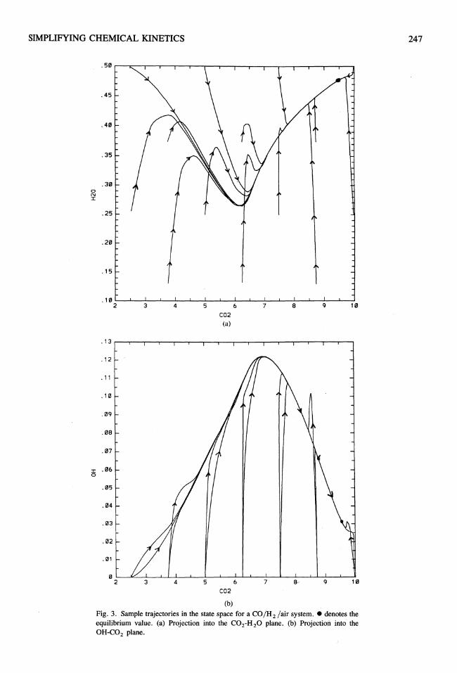
tailed reaction mechanism, which can be found, e.g., in Ref. 19) for the water-gas system for the specific values of pressure, enthalpy, and element composition described in the previous section. Plotted are projections into the CO2 jR20 and the CO2 JOR planes, respectively (it should be noted that this projection leads to some lines that cross, which by no means corresponds to a cross­ing of trajectories). Chemical reaction can be regarded as a movement along those trajectories.

Attracting Manifolds

There is one notable feature that can be seen in Fig. 3, namely the fact that trajectories tend to "bunch" and approach one another far before eqUilibrium is reached. It looks as if there is a low-dimensional manifold (represented by a line in this two-dimensional projection) that has the property that all trajectories tend to approach that manifold, and that on this manifold only slow time scales govern the chemical reaction. In other words, even systems with quite different initial conditions approach common attracting mani­folds.

This observation leads to the central question addressed in this article: Are there low-dimen­sional attracting manifolds in the state space that have the property that if a trajectory is near the manifold, it will remain close to it for all times? We answer this question in the affirmative, and show how such manifolds can be determined and used to simplify chemical kinetics.

MATHEMATICAL MODEL

General Idea

The behavior of a chemical reaction system can be well understood if one looks at distinct points in the state space and analyzes the behavior in the neighborhood. Let us assume that we apply a small perturbation to the system. Row will it respond? The answer can be provided by a modal analysis (Appendix B), which describes the be­havior of the system in a linearized neighborhood of some point in the state space in terms of an analysis of the eigenValues and eigenvectors of the Jacobian of the governing equation system. This analysis reveals that there are n s characteris­tic time scales (given by the eigenvalues of Jhe Jacobian) associated with n s characteristic direc­tions (the corresponding eigenvectors). Now there are three principal possibilities how a system can react to a perturbation, shown schematically in Fig. 4:

1. If we perturb in the direction of an eigenvec­tor whose eigenvalue has a positive real part, the perturbation will increase.

2. If we perturb in the direction of an eigenvec­tor whose eigenvalue is zero (this usually cor­responds to a change of a conserved variable), the perturbation will not change with time.

3. If we perturb in the direction of an eigenvec­tor whose eigenvalue has a negative real part, the perturbation will relax to zero.

It shall be noted that in this example many simplifications had been made (linearization, etc.),

SIMPLIFYING CHEMICAL KINETICS

0 N I

I 0

.50

.45

.40

.35

.30

.25

.20

.15

.10 2 3 4 5 6 7 8 9 10

CO2 (a)

.13

.12

.11

.10

.09

.08

.07

.06

.05

.04

.03

.02

.0'

0 2 3 4 5 6 7 10

CO2

(b)

Fig. 3. Sample trajectories in the state space for a CO/H 2 lair system. - denotes the equilibrium value. (a) Projection into the CO2-H 20 plane. (b) Projection into the OH-C02 plane.

247

248

x Fig. 4. Schematical illustration of the behavior of a dynami­cal system.

but nevertheless it gives an idea of the behavior of real systems. If we look at real chemical systems, sample calculations for a CO/H 2 /02

combustion system show the following: Some eigenvalues are zero, namely those corresponding to the eigenvectors that can be expressed as linear combinations ofthe element vectors (this can also be shown analytically). Almost all other eigenval­ues are negative with values from typically - 10 - 2 to - 10 7 S - 1. Only very few eigenvalues are positive (in the sample calculations at most one eigenvalue was positive). At the equilibrium point all eigenvalues are zero or negative.

Because in chemical reactions a large number of the eigenvalues have large negative values (for an isothermal system, for example, it can be easily shown that the sum of the eigenvalues is always negative), many perturbations of a state (that could be induced, for example, by molecu­lar diffusion) lead to some sort of fast relaxation (which indeed need not lead to the initial state). Furthermore the example (together with Fig. 3) shows that many different initial conditions after some short time (in fact the time scale associated with the smallest eigenvalues) can lead to move­ments within one common subspace of the com­position space.

Further insight is obtained if we look at the time development of a linearized system in the neighborhood of some state 4>0. In Appendix C it is shown for a linearized system that if we iden­tify in the composition space the points where the system is in equilibrium with respect to the fastest

U. MAAS AND S. B. POPE

time scales (i.e., the rates in direction of the eigenvectors with the smallest eigenvalues is zero), we obtain a subspace of the composition space in which all movements correspond to slow time scales. States that are not in this subspace evolve rapidly in time in direction of this sub­space.

The consequences for general systems are as follows: If a subspace in the composition space can be found where the system is "in equilib­rium" with respect to its smallest m eigenvec­tors, this subspace defines a low-dimensional manifold that is characterized by the fact that movements along it are associated with slow time scales and can be used to simplify chemical kinetics.

Mathematical Model

In the previous section it was shown (for simple examples) that based on an eigenvector analysis of the governing equations in a homogeneous chemical reaction system, it is possible to identify some low-dimensional subspaces of the composi­tion space that may be used to simplify the de­scription of complicated chemical systems. This section outlines how the above considerations can be used to construct a method that, given a detailed reaction mechanism, defines a low-di­mensional manifold in the state space with the property that all the movements on this manifold represent slow time-scale processes, and that sys­tems with initial states that do not lie on this manifold evolve rapidly in time in the direction of the manifold.

Consider a chemical reaction system with the governing equations ah 4 at = 0, (7)

ap at = 0, (8)

a4>i wi(h,P,4» i = 1,2, ... , ns ' at p(h,P,4»

(9,10)

or, written in terms of vectors,

a 1/1 at = F(I/I) , (19)

with 1/1 = (h, P, 4>1' 4>2' ... ,4>n )T. s

SIMPLIFYING CHEMICAL KINETICS

For each point in the state space, the eigenval­ues of the Jacobian P", (with components a F; / a if; j) identify the n s + 2 different time scales associated with the movement in the state space. The corresponding eigenvectors describe the "characteristic directions" associated with those time scales. Now the general idea is to look for points in the state space for which components in the directions of certain eigenvectors (in this case those associated with fast time scales) vanish. Because the occurrence of degenerate eigenvalues can complicate the analysis, it is useful to work in a modified eigenvector basis. This modified local basis shall be given as follows: The eigenvectors corresponding to distinct eigenvalues, as well as linearly independent eigenvectors corresponding to a multiple eigenvalue form basis vectors. If an eigenvalue of multiplicity m has less than m linearly independent eigenvectors, or if there is a complex pair of eigenvalues, the vectors, which span the corresponding invariant subspace, shall form basis vectors.

In this way it is possible to construct a basis that spans the whole space of dimension n ::::: n s

+ 2. Now define an nc-dimensional manifold in reaction space by the condition that the compo­nents of the movement in the direction of n f :::::

nr - nc distinct basis vectors vanish. In other words, given the modified basis of eigenvectors V, where V is a matrix with a column partition­ing given by the vectors Vi of the modified eigen­vector basis, ordered according to decreasing values of the real parts of the corresponding eigenvalues

V= (~, v2 JJ (20)

and its inverse V- I :

VI

) , V-I::::: v2

(21 )

un

the equation system

WP(1/t) ::::: 0 (22)

defines the low-dimensional manifold, where W

249

is the n rby-n matrix

U 2+ne+ nc+ 1

W::::: U2+ne+ nc+ 2 (23)

(i.e., W is the matrix formed by the last n f rows of the inverse of the matrix of basis vectors). In this way we define an n c ::::: n r - n rdimensional manifold in the reaction space with the property that for all points on this manifold, the compo­nents of the velocity in direction of the eigenvec­tors corresponding to the n rmost negative eigen­values vanish. Roughly speaking this manifold represents states that are "in equilibrium with respect to the fastest relaxing time scales." How­ever, there is the possibility of some arbitrariness in the formulation, namely if either the eigenval­ues ~+n +n and ~+n +n +1 form a complex pair or ife~:n +n = ~~n ~n + I. In those cases the constructio~ of the ma~if~ld can depend on the choice of the modified basis vectors.

The formulation above would allow the con­struction of a low-dimensional manifold. How­ever, due to poor conditioning (roughly speaking, "nearly linearly-dependent eigenvectors"), nu­merical difficulties could arise [21]. Thus it is useful to work in terms of another basis, the basis of the so-called real Schur vectors [21]. It can be shown that the formulation in this basis is equiva­lent to the formulation above. Furthermore, the basis of real Schur vectors can be easily com­puted [21] and it has the advantage of being orthogonal. Following this approach, the low-di­mensional manifold is constructed as follows:

Let QTp",Q = N denote the real Schur decom­position of the Jacobian, such that the eigenvalues Ai appear in the diagonal of 4N (or in the 2-by-2 blocks in case of complex pairs) in the order of descending real parts. (Such a Schur decomposi­tion always exists and can be calculated efficiently using a modification of the algorithm in Ref. 22.) If Q is written as

q2 (24)

I with qi being the Schur vectors, then the low­dimensional manifold is defined as the set of

250

points in the state space for which

T Q2+ne+nc+ 1

T Q2+ne+ nc+ 2 F(1/;). (25)

QL T denotes the n rby-n matrix, whose row partitioning are the transpose of the Schur vectors Qi with i = 2 + ne + ne + 1,2 + ne + ne + 2, ... , n, or, in other words Q L T is the matrix that is obtained from QT by omitting the first 2 + ne + nc rows, namely the rows correspond­ing to the conserved and the slowly changing variables.

From this construction it can be seen that there is one major difference compared with conven­tional reduced mechanisms, namely the fact that the only restriction imposed on the system is the choice of the dimension n e of the manifold in the reaction space.

Numerical Solution

After the formUlation for the construction of the low-dimensional manifold has been given, there is need for a numerical method that allows the computation. In general, the manifold in the reac­tion subspace can (at least piecewise) be parametrized by ne( = nr - nf ) coordinates.

Thus together with Eq. 25, 2 + ne + ne pa­rameters define the low-dimension manifold in the state space. The task of identifying the low­dimensional manifold consists of solving the pa­rameter equations

with P(1/;T) being 2 + ne + ne additional pa­rameter equations necessary to complete the equa­tion system. The choice of those equations influ­ences problems of existence and uniqueness of a solution to Eq. 26, but not the construction ofthe manifold itself. Because we are treating closed, adiabatic, isobaric systems here, 2 + ne of the

. parameter equations are readily obtained, namely

U. MAAS AND S. B. POPE

by specifying

0= h - T h ,

0= P - Tp ,

i=I,2, ... ,ne , (27)

that is, by using the equations fixing enthalpy, pressure, and element composition. The choice of the remaining n e parameter equations cannot be performed in such an easy way in order to guar­antee existence and uniqueness.

To summarize, in order to obtain the manifold, we now have to solve the equation system

0= QLT(1/;)F(1/;) ,

0= g(1/;, Te),

0= h( 1/;, Te),

(28)

(29)

(30)

where Eq. 28 gives the definition equations for the manifold, Eq. 29 the parameter equations that fix the conserved variables, and Eq. 30 the re­maining parameter equations, which have yet to be specified. The parameters Te and the corre­sponding equations can be chosen quite arbitrarily and may, for example, be the temperature, spe­cific mole numbers, specific element mole num­bers, concentrations, or even linear combinations of them. Their definition has no influence on the manifold itself, but only allows some parametri­zation. If we use specific mole numbers in order to parametrize the manifold, this corresponds to a projection of the manifold onto coordinates in the natural basis of the state space. The equation system 30 then reads

cPi - T<I>i = 0 (31)

for ne specific species. Now after the equation system has been com-t

pleted, there are several ways of finding solu­tions. The simplest way is to look for solutions for fixed values of the parameters, that is, solve Eq. 26 by Newton's method.

In order to illustrate this, let us take the CO/H 2 lair combustion system as an example. U sing detailed chemistry, the dimension of the governing ordinary differential equation system is 15, with the enthalpy h, the pressure P, and the specific mole numbers of the species H 2' CO, 02' N2, CO2, H20, H, 0, OH, H02, HCO, .

SIMPLIFYING CHEMICAL KINETICS

CHzO, and HzOz as dependent variables. Be­cause the reaction system is said to be closed, adiabatic, homogeneous, and isobaric, there are six conserved variables, namely, the pressure, the enthalpy, and the specific element mole numbers of H, 0, C, and N. Thus the dimension of the

251

reaction space is n - n e - 2 = 9. If we want to Y reduce the dimension of the reaction space to let us say two, two parameters have to be defined. The choice is quite arbitrary; thus assume that the specific mole numbers of HzO and COz are the parameters. In this way we would end up with the equation system

0= h - Th'

0= P - Tp ,

o = XH ( <1» - T H ,

0= Xo(<I» - TO'

0= Xe(<I» - Te ,

0= XN(<I» - TN'

0= <l>H20 - T H20 ,

0= cf>e02 - Te0 2 ,

(32)

which, for given reference values T, calculates points that lie on the manifold. This defines a two-dimensional manifold in the reaction space with the reaction progress variables being ¢H 20

and cf>e02 ' If this equation system is solved for varying values of the parameters, a table of points on the low-dimensional manifold is obtained. Certain difficulties may arise, however, depend­ing on the choice of parameters, which can be seen from Fig. 5. It shows an arbitrary example for a one-dimensional manifold in a two-dimen­sional space. If x is chosen as a parameter, in some domains a unique mapping could not be defined. However, if we choose y as the parame­ter, the problem is easily solved in this example. Another problem is that the theoretically accessi­ble values for the parameters do not necessarily need to be values for which points on the mani­fold exist. This can be seen from a simple exam­ple. Consider the CO/Hz lair system discussed above. Theoretically (assuming a stoichiometric mixture) all hydrogen could be present as HzO. But at high temperatures the construction of the

x Fig. 5. Mapping of a one-dimensional manifold.

manifold would always determine a certain amount of hydrogen which appears as H or OH. All those problems can be easily avoided because the choice of the parametrization does not influ­ence the construction of the manifold. Thus arc­length continuation methods can be used to solve Eq. 26 [27].

In this work we use several different ap­proaches to solve Eq. 26. Usually, the solution is performed by Newton's method. In case of con­vergence problems due to bad initial guesses, an iterative approach is used. It can be outlined as follows:

Start with an initial guess of the state variables o (h, P, <1» that fulfills the algebraic equations P(if;, r) of Eq. 26. For i = 0,1,2, ...

Compute the Jacobian iF", of the governing equation system and the Real Schur decomposi­tion iQTiF/Q = N for given iif; =i(h, P,<I». Solve

P(if;,r) =0, (33)

iQLT:~ =iQLTF(if;), (34)

until a steady state is obtained. If II i+ 1 if; - i if; II < E accept solution, set if; = i+ 1 if; and leave loop.

The solution ofthe differential/algebraic equation system 33-34 is performed by an extrapolation method [23, 24].

Additionally, if problems in the parametriza­tion occur as described above, the arc-length

252

continuation methods ALCON 1 [28] or PITCON [29] can be used.

However, it would be desirable to develop a general procedure, that is, a general arc-length continuation method with an arbitrary number of parameters, capable of avoiding those problems in the numerical solution.

RESULTS

Given a detailed reaction mechanism, the method presented so far allows the automatic generation of low-dimensional manifolds in composition space, which can be used to obtain simplified models for chemical reaction systems. In order to show the validity of the approach, sample calcula­tions for low-dimensional manifolds, as well as for trajectories in the state space have been per­formed. The system considered here is a carbon monoxide-hydrogen-air combustion system that has been discussed in detail in a previous section. Calculations using the method described in this article are performed in order to determine one­and two-dimensional manifolds in the reaction space. The reason for the restriction to such low dimensions is only because of problems in the visualization of the results. Higher-dimensional manifolds can easily be calculated, too. Sample trajectories are calculated by solving the system of governing equations for an adiabatic, isobaric, homogeneous closed reaction system for varying initial conditions. Details can be found in Refs. 18 or 25. All calculations (low-dimensional mani­fold as well as sample trajectories) are based on a detailed reaction mechanism consisting of 13 species and 67 elementary reactions listed in Table 1 (see, e.g., Ref. 19 for details and further references) .

One-Dimensional Manifolds

A comparison of one-dimensional manifolds in the reaction space obtained by the method de­scribed in this article with manifolds obtained from a conventional reduced mechanism has been performed in order to point out the difference between these two methods. The reaction progress variable is chosen to be the specific mole number of CO2 • The conventional reduced mechanism is obtained in the following way: For points on the calculated one-dimensional manifold in the state

U. MAAS AND S. B. POPE

space an analysis of the reaction mechanism is performed, that is, based on a detailed mecha­nism [19], the reactions that are in partial equilib­rium as well as the species that are in quasi­steady-state are determined. The results are used to form the algebraic constraints needed to con­struct the manifold. At the conditions that are investigated, H02 , HCO, CH 20, and H 20 2 are almost in quasi-steady-state, and the reactions

H + °2 ...... OH + 0,

0+ H2 ...... OH + H,

OH + H2 ...... H 20 + H,

CO + OH + M ...... CO2 + H

are more or less in partial equilibrium. Using those constraints, the compositions on the mani­fold for the reduced mechanism are calculated using Newton's method.

In this way, for fixed values of the enthalpy, the pressure, and the element mass fractions, all other state variables are explicitly given as func­tions of the reaction progress variable alone.

Figures 6a and 6b show examples of this map­ping for the specific mole numbers of H 20 and H. It can be seen that at temperatures higher than about 1700 K (corresponding to a specific mole number for CO2 of about 6 for this particular mixture) the two manifolds agree quite well. Be­low this temperature there seems to be a change of the reaction paths that cannot be accounted for by the quasi-steady-state and partial eqUilibrium assumptions made in the conventional reduced mechanism. In order to show that the manifold obtained by the above method describes the reac­tion system better than the one obtained with the conventional reduced mechanism, sample calcula­tions of trajectories in the state space (based on a detailed reaction mechanism [19]) are performed. Many different initial conditions are used, corre­sponding to pure mixtures of H 2, 02' CO, CO2 ,4

H 20, and N2 as well as to mixtures with large amounts of hydrogen atoms added. Plots of the two manifolds together with the trajectories are shown in Figs. 7a and 7b. Plotted are the specific mole numbers of H20 and H versus the reaction progress variable (specific mole number of CO2),

respectively. It can be seen that the trajectories approach the manifold, which is calculated using the method described in this article. Even in

SIMPLIFYING CHEMICAL KINETICS

0 N I

:r:

.45

.40

.35

.30

.25

.20

.15

intrinsic low-dimensional manifold

conventional reduced mechanism

.10UU~UU~LU~LU~LUUUlLUU~UU~LU~~LU~LU~lLUU~LU~U 2.5 3.0 3.5 4.0 4.5 5.0 5.5 6.0 6.5 7.0 7.5 B.0 8.5 9.0

.65

.60

.55

.50

.45

.40

.35

.30

.25

.20

.15

.10

.05

C02 (a)

intrinsic

conventional

reduced mechanism

low-dimensional manifold

o ~~~~~~~uu~~~~~~~~UU~UULU~LU~~LUW 2.5 3.0 3.5 4.0 4.5 5.0 5.5 6.0 6.5 7.0 7.5 B.0 '8.5 9.0

C02

(b) Fig. 6. (a) Plot of the one-dimensional manifold for the specific mole number of H 20, • denotes the equilibrium value, (b) Plot of the one-dimensional manifold for the specific mole number of H, • denotes the equilibrium value,

253

254

. 5 III

.45

.4"

.35

.30 0 N I

.25

.20

.15

·Hl 2.5 3.0 3.5

. 7 III

.65

. 6 III

.55

. 5 III

.45

.4"

.35

I .3"

.25

.2"

.15

. 1"

.05

Ii! 2.5 3.1i! 3.5

intrinsic low-dimensional manifold

4.0 4.5 5.0 5.5 6.0 CO2 (a)

4.1i! 4.5 5.1i! CO2 (b)

U. MAAS AND S. B. POPE

conventional

reduced mechanism

6.5 7.0 7.5 9.0

conventional

reduced mechanism

9.5 9.0

Fig. 7. (a) Plot of the one-dimensional manifold for the specific mole number of H 20 together with sample trajectories. • denotes the equilibrium value. (b) Plot of the one-dimensional manifold for the specific mole number of H together with sample trajectories .• denotes the equilibrium value.

SIMPLIFYING CHEMICAL KINETICS

regions (low temperatures) where a conventional reduced mechanism with such a small number of steps fails, the manifold describes the reaction system quite well.

One aspect that those pictures do not show is the speed with which the trajectories approach the low-dimensional manifold. In fact (as is shown later for examples with two reaction progress variables) it only takes a short time for the trajec­tories to approach the manifold, compared with the time associated with the following movement along the manifold. One further effect can be seen in the plots. In regions of low temperatures, the trajectories approach the manifold, but only "merge' , with it as soon as the temperature increases. Thus it might be necessary to take into account another reaction progress variable (in­creasing the dimension of the reaction space to two) at low temperatures. In fact, calculations show (see below) that the low-temperature range can be described much better if two reaction progress variables are defined.

Two-Dimensional Manifolds

For the two-dimensional manifolds in ~e reaction space the specific mole numbers of CO2 and H 20 have been chosen as parameters. Thus (given specific values for the enthalpy, the pressure, and the specific element mole numbers) the numerical method provides values for the specific mole numbers of all species as functions of cPco2 and cPH 20' The results then can be visualized in a three-dimensional plot of the chosen variable ver­sus the two reaction progress variables.

Figures 8a and 8b show plots of the two-di­mensional manifolds for the specific mole num­bers of H and OH, respectively. However, the method produces such manifolds for all the dif­ferent species in the reaction system. In addition to the two-dimensional manifolds (represented by the nets of lines), the one-dimensional mani­folds (described above), which lie on the two­dimensional manifolds, have been plotted and can be seen as lines on the surfaces. There are several important features that should be mentioned: First the manifolds are nonlinear. This can be ex­pected, because the chemistry introduces nonlin­ear terms in the governing equation system. Far more interesting is the fact that there exist local maxima and minima in the plots (e.g., the mini­mum in the plot of the OH specific mole num-

255

(a)

(b)

Fig. 8. (a) Plot of the two-dimensional manifold for the specific mole number of H .• denotes the equilibrium value. Plotted are specific mole numbers in the range of 1.85-9.32 for CO2 , 0.096-0.496 for H 20, 0.0-0.855 for H. The arrows at the axes denote increasing values of the variables .• denotes the equilibrium value. (b) Plot of the two-dimensional manifold for the specific mole number of OH .• denotes the equilibrium value. Plotted are specific mole numbers in the range of 1.85-9.32 for CO2 , 0.096-0.496 for H20, 0.0-0.224 for OH. The arrows at the axes denote increasing values of the variables .• denotes the eqUilibrium value.

bers). In these regions there seems to be a change of the reaction paths governing the chemical ki­netics, which is recognized fY the method.

In the same way as for the one-dimensional manifolds, the significance of these manifolds is

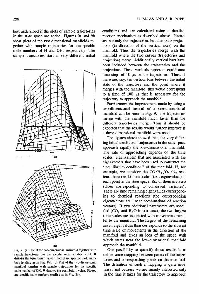
256

best understood if the plots of sample trajectories in the state space are added. Figures 9a and 9b show plots of the two-dimensional manifolds to­gether with sample trajectories for the specific mole numbers of H and OH, respectively. The sample trajectories start at very different initial

t

(a)

r

(b)

Fig. 9. (a) Plot of the two-dimensional manifold together with sample trajectories for the specific mole number of H. • d'rtotIts the bquilibrium value: Plotted are specific mole num­bers (scaling as in Fig. 8a). (b) Plot of the two-dimensional manifold together with sample trajectories for the specific mole number of OH .• denotes the equilibrium value. Plotted are specific mole numbers (scaling as in Fig. 8b).

U. MAAS AND S. B. POPE

conditions and are calculated using a detailed reaction mechanism as described above. Plotted are not only the trajectories, but also their projec­tions (in direction of the vertical axes) on the manifold. Thus the trajectories merge with the manifold where the two curves (trajectories and projection) merge. Additionally vertical bars have been included between the trajectories and the projections. These verticals represent equidistant time steps of 10 p,s on the trajectories. Thus, if there are, say, ten vertical bars between the initial state of the trajectory and the point where it merges with the manifold, this would correspond to a time of 100 p,s that is necessary for the trajectory to approach the manifold.

Furthermore the improvement made by using a two-dimensional instead of a one-dimensional manifold can be seen in Fig. 9. The trajectories merge with the manifold much faster than the different trajectories merge. Thus it should be expected that the results would further improve if a three-dimensional manifold were used.

The figures above showed that, for very differ­ing initial conditions, trajectories in the state space approach rapidly the low-dimensional manifold. The rate of approaching depends on the time scales (eigenvalues) that are associated with the eigenvectors that have been used to construct the "equilibrium condition" of the manifold. If, for example, we consider the CO/H2 /02 /N2 sys­tem, there are 15 time scales (i.e., eigenvalues) at each point in the state space. Six of them are zero (those corresponding to conserved variables). There are nine remaining eigenvalues correspond­ing to chemical reactions (the corresponding eigenvectors are linear combinations of reaction vectors). If two additional parameters are speci­fied (C02 and H20 in our case), the two largest time scales are associated with movements paral­lel to the manifold. The largest of the remaining seven eigenvalues then corresponds to the slowest time scale of movements in the direction of the manifold and gives an idea of the speed with which states near the low-dimensional manifold approach the manifold.

One possibility to quantify those results is to define some mapping between points of the trajec­tories and corresponding points on the manifold. The definition of such a mapping is quite arbi­trary, and because we are mainly interested only in the time it takes for the trajectory to approach

SIMPLIFYING CHEMICAL KINETICS

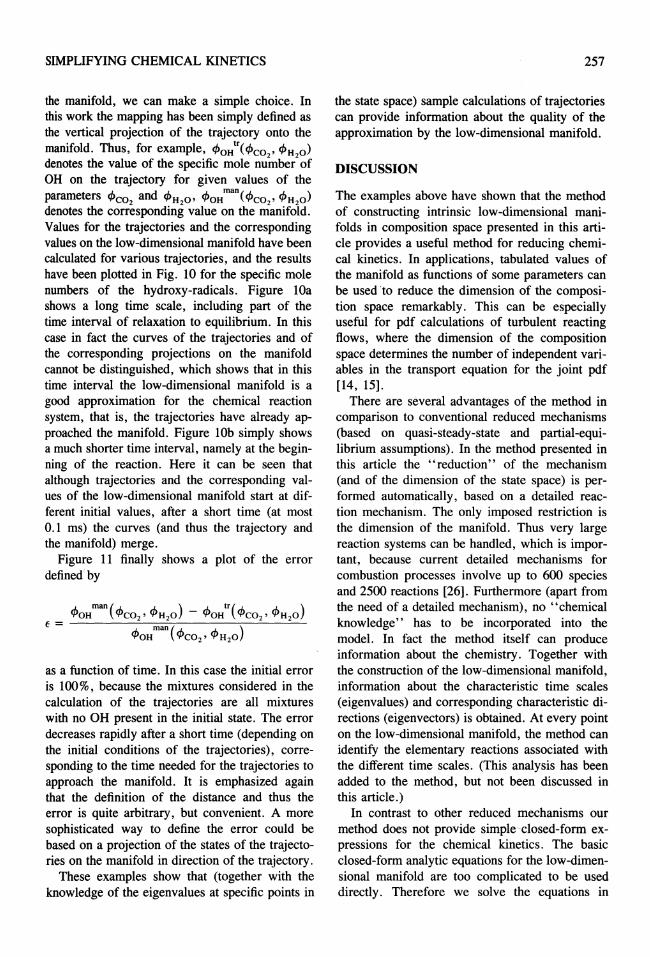
the manifold, we can make a simple choice. In this work the mapping has been simply defined as the vertical projection of the trajectory onto the manifold. Thus, for example, cf>oHtr( cf>c02 , cf>H 20) denotes the value of the specific mole number of OH on the trajectory for given values of the parameters cf>co2 and cf>H 20' cf>oH mao ( cf>co2 , cf>H 20) denotes the corresponding value on the manifold. Values for the trajectories and the corresponding values on the low-dimensional manifold have been calculated for various trajectories, and the results have been plotted in Fig. 10 for the specific mole numbers of the hydroxy-radicals. Figure lOa shows a long time scale, including part of the time interval of relaxation to equilibrium. In this case in fact the curves of the trajectories and of the corresponding projections on the manifold cannot be distinguished, which shows that in this time interval the low-dimensional manifold is a good approximation for the chemical reaction system, that is, the trajectories have already ap­proached the manifold. Figure lOb simply shows a much shorter time interval, namely at the begin­ning of the reaction. Here it can be seen that although trajectories and the corresponding val­ues of the low-dimensional manifold start at dif­ferent initial values, after a short time (at most 0.1 ms) the curves (and thus the trajectory and the manifold) merge.

Figure 11 finally shows a plot of the error defined by

f' = cf>OH mao ( cf>co2 , cf>H 20) - cf>oHtr( cf>co2 , cf>H 20)

cf>OH mao ( cf>co2 , cf>H 20)

as a function of time. In this case the initial error is 100%, because the mixtures considered in the calculation of the trajectories are all mixtures with no OH present in the initial state. The error decreases rapidly after a short time (depending on the initial conditions of the trajectories), corre­sponding to the time needed for the trajectories to approach the manifold. It is emphasized again that the definition of the distance and thus the error is quite arbitrary, but convenient. A more sophisticated way to define the error could be based on a projection of the states of the trajecto­ries on the manifold in direction of the trajectory.

These examples show that (together with the knowledge of the eigenvalues at specific points in

257

the state space) sample calculations of trajectories can provide information about the quality of the approximation by the low-dimensional manifold.

DISCUSSION

The examples above have shown that the method of constructing intrinsic low-dimensional mani­folds in composition space presented in this arti­cle provides a useful method for reducing chemi­cal kinetics. In applications, tabulated values of the manifold as functions of some parameters can be used to reduce the dimension of the composi­tion space remarkably. This can be especially useful for pdf calculations of turbulent reacting flows, where the dimension of the composition space determines the number of independent vari­ables in the transport equation for the joint pdf [14, 15].

There are several advantages of the method in comparison to conventional reduced mechanisms (based on quasi-steady-state and partial-equi­librium assumptions). In the method presented in this article the "reduction" of the mechanism (and of the dimension of the state space) is per­formed automatically, based on a detailed reac­tion mechanism. The only imposed restriction is the dimension of the manifold. Thus very large reaction systems can be handled, which is impor­tant, because current detailed mechanisms for combustion processes involve up to 600 species and 2500 reactions [26]. Furthermore (apart from the need of a detailed mechanism), no "chemical knowledge" has to be incorporated into the model. In fact the method itself can produce information about the chemistry. Together with the construction of the low-dimensional manifold, information about the characteristic time scales (eigenvalues) and corresponding characteristic di­rections (eigenvectors) is obtained. At every point on the low-dimensional manifold, the method can identify the elementary reactions associated with the different time scales. (This analysis has been added to the method, but not been discussed in this article.)

In contrast to other reduced mechanisms our method does not provide simple closed-form ex­pressions for the chemical kinetics. The basic closed-form analytic equations for the low-dimen­sional manifold are too complicated to be used directly. Therefore we solve the equations in

258

.21il

.18

.16

.14

.12

.11il

I 0

.1il8

.1il6

.1il1il1il4 .1il1il1il6

.20

.18

.16

.14

.12

.10

I 0

.08

.06

.1il4

Iil <SI

;S; ;S; 5l IS>

~ ~

.1il1il1il8 tlseci (a)

;S; ;S; 5l 5l

~ ~

tlseci (b)

.lilll11il

;S; 5l

~

U. MAAS AND S. B. POPE

.1il1il12 .1il1il14 .1il1il16

.0 (Xl 5l N N M 5l 5l 5l IS> 5l 5l

~ ~ ~

Fig. 10. (a) Plot of the specific mole number of H from sample trajectories and their projection on the manifold versus time. (b) Plot of the specific mole number of OH from sample trajectories and their projection on the manifold versus time.

SIMPLIFYING CHEMICAL KINETICS 259

1.0

.9

.9

.7

.6

.5

is .4

.3

.2

.1

0

- . 1 !--'-.:::IS!:::SS==2'-.:::Bs!:::ee:74'-.:::8B!:::se:76'-.:::se!:::e.==e'-.:::le!:::"=-=I'-.:::ee!:::"=-=2'-.:::B.!:::e,:-74'-.:::'B!:::B,:76'-.:::.s!:::.,=-=a'-.:::,s!:::'2==.'-.:::"!:::S2==2'-.:::S'!:::'2:74'-.=81126

tlsec)

Fig. 11. Plot of the normed distance between sample trajectories and the manifold (see text).

order to tabulate the manifolds for subsequent use. This kind of representation of the results is not very convenient from a kineticist's viewpoint. As a consequence sensitivity results cannot be obtained directly. But our method is not aimed at obtaining kinetic details of a combustion system (here detailed numerical calculations of homoge­neous ignition and one-dimensional laminar flames will very often provide the best insight). Our aim is to couple chemical kinetics with very compli­cated flow problems (like pdf methods for turbu­lent flows). In many of those models the computa­tional effort forces a tabulation of the chemical kinetics in order to be able to treat not only idealized systems (like one-dimensional flames), but technically relevant three-dimensional pro­cesses in complex geometries. In principle all the method does is to uncouple fast time scales in the chemical kinetics and assume them to be in equi­librium. Thus, if one knows the "physical" time scales of the combustion process considered (e.g., diffusion, turbulent time scales), the method also allows one to decouple those fast chemical time scales that are much faster than the "physical"

time scales in systems other than homogeneous systems.

Although the methods of the approach dis­cussed in this article are similar to those used by Lam and Goussis [11-13] (namely the dynamic systems theory), the aim and the realization of our approach is different in many aspects. Lam and Goussis use Computational Singular Pertur­bation for the analysis of distinct reaction trajec­tories. In their method they use refined basis vectors in order to decouple slow and fast time­scales. In this way they are able to integrate the stiff differential equation systems of chemical ki­netics by means of explicit solvers with a very high accuracy [12]. At the same time (by identify­ing reaction groups) they obtain useful informa­tion about the chemical kinetics of the system. Our aim is quite different and motivated by the need of reduced schemes in turbulence modeling, especially in pdf methods. In those methods there is a high demand for reduced schemes that allow the treatment of complex reaction systems by a low-dimensional state space, that is, schemes that describe the reaction system in terms of only a

260

few state variables. Thus, in this case, it is neces­sary not to look at distinct trajectories in the reaction space, but to reduce the dimension of the state space globally. By means of the method of constructing intrinsic low-dimensional manifolds, we are able to describe the reaction space in terms of only a few parameters (i.e., controlling variables). Having determined such low-dimen­sional manifolds, it is possible to tabulate the results. In this way, for given values of the controlling variables, all the remaining state vari­ables are explicitly given. The results then can be used to calculate the temporal development of the chemical states (by means of solving the chemical rate equations using detailed chemistry), which is used by a table-lookup, for example in pdf meth­ods [15]. The computational cost for the calcula­tion of the low-dimensional manifold and the integration of the corresponding rate equations are a small expense compared with the subse­quent use in turbulence calculations.

The results presented in this article give only some examples of the potential of the method. Further work includes the implementation of the method in laminar and turbulent flame calcula­tions, that is, the extension to nonhomogeneous problems [30]. One important question to be ad­dressed is the choice of the parametrizing vari­ables, which (as described above) does not influ­ence the construction of the manifold, but only determines the way of mapping. Finally the nu­merical method that has been developed to deter­mine the intrinsic manifold can be refined in several respects.

Financial support by General Electric is gratefully acknowledged. U. Maas is grateful to the Deutsche Forschungsgemeinschafi for a postdoctorate fellowship. The authors wish to thank Prof. J. Warnatz for helpful discus­sions.

REFERENCES

1. Dixon-Lewis, G., David, T., Gaskell, P. H., Fukutani, S., Jinno, H., Miller, 1. A., Kee, R. J., Smooke, M. D., Peters, N., Effelsberg, E., Warnatz, J., and Behrendt, F., Twentieth Symposium (International) on Combustion, The Combustion Institute, Pittsburgh, 1985, p. 1893.

2. Warnatz, J., Eighteenth Symposium (International) on Combustion, The Combustion Institute, Pittsburgh, 1981, p. 369.

U. MAAS AND S. B. POPE

3. Peters, N., and Warnatz, J., Eds., Numerical Methods in Laminar Flame Propagation, Vieweg, Braun­schweig, 1982.

4. Smooke, M. D., Mitchell, R. E., and Keyes, D. E., Combust. Sci. Technol. 67:85 (1989).

5. Chen, J-Y., and Dibble, R. W., in Reduced Kinetic Mechanisms and Asymptotic Approximations for Methane-Air Flames (M. D. Smooke, Ed.), in press.

6. Peters, N., and Kee, R. J., Combust. Flame 68:17 (1987).

7. Bilger, R. W., and Kee, R. J., Western States Fall Meeting, The Combustion Institute, paper no. 87-85 (1987).

8. Chen, J-Y., Combust. Sci. Technol. 57:89 (1988). 9. Smooke, M. D., Ed., Reduced Kinetic Mechanisms

and Asymptotic Approximations for Methane-Air Flames, in press.

10. Keck, J. C., Twenty-Second Symposium (Interna­tional) on Combustion, The Combustion Institute, Pittsburgh, 1989, p. 1705.

11. Lam, S. H., and Goussis, D. A., Twenty-Second Sym­posium (International) on Combustion, The Com­bustion Institute, Pittsburgh, 1989, p. 931.

12. Lam, S. H., and Goussis, D. A., Technical Report # 1864(a)-MAE, Princeton University, 1990.

13. Lam, S. H., and Goussis, D. A., Technical Report # 1864(a)-MAE, Princeton University, 1991.

14. Pope, S. B., Prog. Ener. Combust. Sci. 11:119 (1985).

15. Pope, S. B., and Correa, S. M., Twenty-First Sympo­sium (International) on Combustion, The Combus­tion Institute, Pittsburgh, 1986, p. 1341.

16. Hirschfelder, J. 0., and Curtiss, C. F., Theory of Propagation of Flames, Third Symposium on Com­bustion, Flame and Explosion Phenomena, Williams & Wilkins, Baltimore, 1949, pp. 121-127.

17. Bird, R. E., Stewart, W. E., and Lightfoot, E. N., Transport Phenomena, Wiley Interscience, New York, 1960.

18. Warnatz, 1., and Maas, U., in Numerical and Applied Mathematics (W. F. Ames, ed.), J. C. Baltzer AG, 1989, pp. 151-157.

19. Maas, U., and Warnatz, J., Twenty-Second Sympo­sium (International) on Combustion, The Combus­tion Institute, Pittsburgh, 1989, p. 1,695.

20. Brauer, F., and Nohel, J. A., The Qualitative Theory of Ordinary Differential Equations, Dover, New York, 1989.

21. Golub, G. H., and van Loan, C. F., Matrix Computa­tions, 2nd ed., Johns Hopkins University Press, Balti­more, 1989.

22. Stewart, G. W., ACM Trans. Math. Soft. 2:275-280 (1976).

23. Deuflhard, P., Hairer, E., and Zugck, J., University of Heidelberg, SFB 123: Technical Report 318, University of Heidelberg, Heidelberg, Germany, 1985.

24. Deuflhard, P., and Nowak, U., SFB 123 Technical Report 332, University of Heidelberg, Heidelberg, Ger­many, 1985.

25. Maas, U., and Warnatz, 1., Combust. Flame 74:53 (1988).

SIMPLIFYING CHEMICAL KINETICS

26. Chevalier, C., Warnatz, J., and Melenk, H., submitted. 27. Fox, R., personal communication. 28. Deufthard, P., Fiedler, B., and Kunkel, P., University

of Heidelberg, SFB 123, Technical Report 278, 1984. 29. Rheinboldt, W., and Burkardt, J., ACM Trans. Math.

Soft. 9:215-241 (1983). 30. Maas, U., and Pope, S. B., in preparation.

Received 23 October 1990; revised 28 August 1991

APPENDIX A: PARTIAL-EQUILIBRIUM AND STEADY-STATE ASSUMPTIONS

Alternative Bases

The composition space <I> is an ns-Jimensional space. The realizable subset is an (ns - 1)­dimensional subspace (due to the constraint that the mass fractions sum to unity). In the composi­tion space <I> some distinct vectors have special meanings: a movement along a reaction vector Pi

corresponds to a (possibly physically unrealistic) chemical reaction; a movement along an element vector p, i corresponds to a change of element composition (which is not allowed in chemical reactions). If we restrict to a given element com­position, an (n s - n e)-dimensional linear sub­space R of the composition space <I> is defined, which contains all states that can be changed into another by chemical reaction. This subspace R shall be called the reaction subspace. It is spanned by reaction vectors Pi'

For further analysis it is useful to describe the state not in terms of specific mole numbers, but in terms of some other basis. Now, the composi­tion space can be described in any convenient basis that spans the space [11]. For example, take a basis formed by n s linearly independent vec­tors. The change of the basis is given by

Bs = 4>, (AI)

where s are the new variables and B is the transformation matrix, with the column partition­ing given by the basis vectors:

(A2)

261

The inverse of B, B- 1, which is used for the transformation, is denoted by

(A3)

The system of governing equations (Eq. 9) is transformed according to

s = B- 10(s, h, p) = o. (A4)

(From now on, if an inverse of a matrix is formed, it shall always be assumed that the ma­trix is not singular.)

Separation Into Conserved and" Reacting" Scalars

If B is a basis formed by n e element composition vectors and n r = n s - n e linearly independent reaction vectors, that is,

the equation system is transformed to

o

+), (AS)

(A6)

Noting that the first ne components of s are the coordinates ~-i in the element space E (spanned by p,;), while the remaining n r components of s are coordinates ri in the reaction space R,

SI ~I

sne ~ne (A7) sne+1 rl

sns rn,

262

the equation system reads

~ = 0,

r = f( h, P, s) . (AS)

This means that in this basis we automatically separate into conserved and reactive variables, that is, ne algebraic equations confine the chemi­cal reaction to the reaction space, n r differential equations describe the movement within the reac­tion space.

Partial-Equilibrium Assumption

In partial-equilibrium schemes a set of (linearly independent) reactions is specified, which are as­sumed to have equal forward and reverse rates. To begin, for simplicity, we consider the partial­equilibrium assumption applied to reaction 1. By assumption, the forward and reverse rates of reaction 1 balance, and hence the reaction rate is zero:

(A9)

where b i is the ith row vector of the inverse B - , of the transformation matrix. In the nr-dimen­sional reaction space R, the points r [recall s = (~, r)] that satisfy this nonlinear algebraic equa­tion form an ( n r - 1 )-dimensional nonlinear manifold, Pl. More generally if the first n p

reactions (np =s; n r ) are in partial equilibrium, then the np equations Ii = 0, i = 1,2, ... , np define an (n r - np)-dimensional manifold Pnp

in R. The idea behind the partial equilibrium as­

sumption is that, except near Pn , the reaction • p

rates Ii' 1= 1,2, ... , np are very large, caus-ing the composition rapidly to approach the mani­fold Pn . This can be formalized by defining trajectories (from any initial composition) by the equations

r=

A

A

A (AI0)

U. MAAS AND S. B. POPE

in the limit as A -+ 00. Thus, in the first in­finitesimal time interval, r n +" r n + 2' . . . , r n

~ p r change infinitesimally, while r" r 2' ... , r n

change to a point on the manifold Pn , so that p

Ali is finite (i.e., Ii = 0, i = 1,2, ... , np ).

Steady-State Assumption

In steady-state assumptions the time derivative of the concentrations of n q distinct species is said to vanish, the species then obtaining steady states. Let the species be ordered so that the first n q are in the steady state.

In this case the transformation matrix B is not only formed by the element and the reaction vectors, but also by the species vectors ai-the natural basis of the composition space:

(All)

These are unit vectors that are orthogonal neither to the element, nor to the reaction vectors.

( ,! ... B= ,....,

I ';, ) (A12)

The equations for the steady-state assumptions read

i= 1,2, ... ,nq , (A13)

where b i is the ith row vector of the inverse B - , of the transformation matrix. Thus, if nq species (nq =s; n r ) are assumed to be in steady state, then the nq equations (A 13) define an (n r - n q)­dimensional manifold Qn in R.

q

Combined Partial-Equilibrium and Steady­State Assumption

Of course quasi-steady-state and partial-equi­librium assumptions are usually combined. Thus the dimension of the reaction manifold (i.e., the subspace in which reaction proceeds) of a system with ns species, ne different elements, nq quasi­steady-state and n p partial eqUilibrium assump­tions is given by nm = ns - ne - np - n q. As a result, if we have, for example, a one-step mechanism, this corresponds to a single line in

SIMPLIFYING CHEMICAL KINETICS

the reaction space, a two-step mechanism corre­sponds to a surface, and so on.

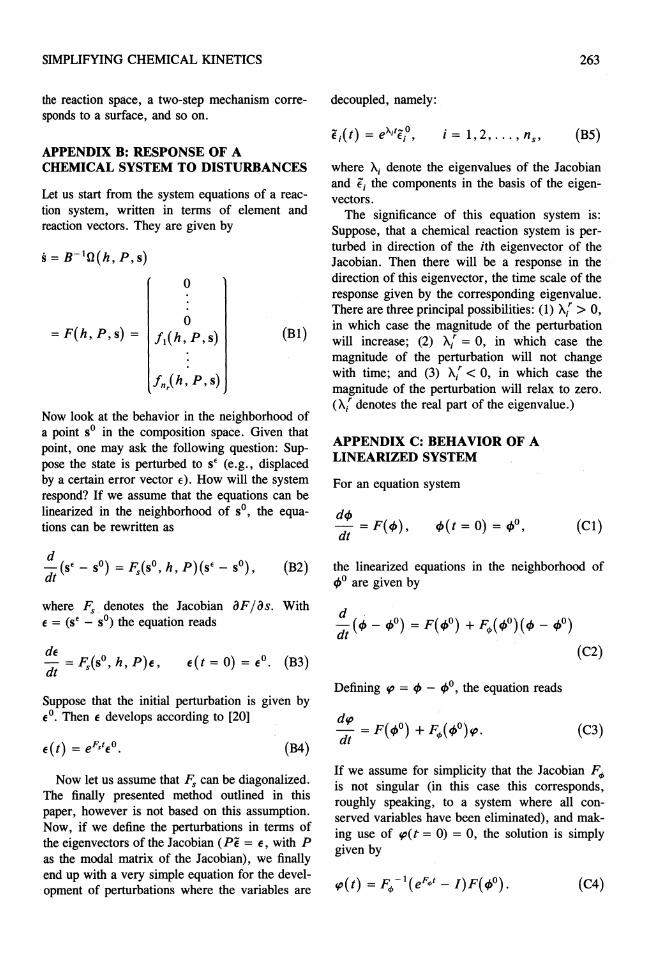
APPENDIX B: RESPONSE OF A CHEMICAL SYSTEM TO DISTURBANCES

Let us start from the system equations of a reac­tion system, written in terms of element and reaction vectors. They are given by

s = B-10(h, P,s)

o

o =F(h,P,s)= i1(h,P,s) (Bl)

Now look at the behavior in the neighborhood of a point SO in the composition space. Given that point, one may ask the following question: Sup­pose the state is perturbed to s· (e.g., displaced by a certain error vector E). How will the system respond? If we assume that the equations can be linearized in the neighborhood of SO, the equa­tions can be rewritten as

(B2)

where F;, denotes the Jacobian aF / as. With E = (s' - so) the equation reads

de ° - = F;,(s ,h, P)e, dt

e(t = 0) = eO. (B3)

Suppose that the initial perturbation is given by eO• Then e develops according to [20]

(B4)

Now let us assume that F;, can be diagonalized. The finally presented method outlined in this paper, however is not based on this assumption. Now, if we define the perturbations in terms of the eigenvectors of the Jacobian (PE = e, with P as the modal matrix of the Jacobian), we finally end up with a very simple equation for the devel­opment of perturbations where the variables are

263

decoupled, namely:

i=1,2, ... ,ns ' (B5)

where Ai denote the eigenvalues of the Jacobian and Ei the components in the basis of the eigen­vectors.

The significance of this equation system is: Suppose, that a chemical reaction system is per­turbed in direction of the ith eigenvector of the Jacobian. Then there will be a response in the direction of this eigenvector, the time scale of the response given by the corresponding eigenvalue. There are three principal possibilities: (1) A( > 0, in which case the magnitude of the perturbation will increase; (2) A( = 0, in which case the magnitude of the perturbation will not change with time; and (3) A( < 0, in which case the magnitude of the perturbation will relax to zero. (A( denotes the real part of the eigenvalue.)

APPENDIX C: BEHAVIOR OF A LINEARIZED SYSTEM

For an equation system

dq, - = F(q,) dt '

q,(t = 0) = q,0, (Cl)

the linearized equations in the neighborhood of q,0 are given by

Defining fP = q, - q,0, the equation reads

(C3)

If we assume for simplicity that the Jacobian F", is not singular (in this case this corresponds, roughly speaking, to a system where all con­served variables have been eliminated), and mak­ing use of fP(t = 0) = 0, the solution is simply given by

(C4)

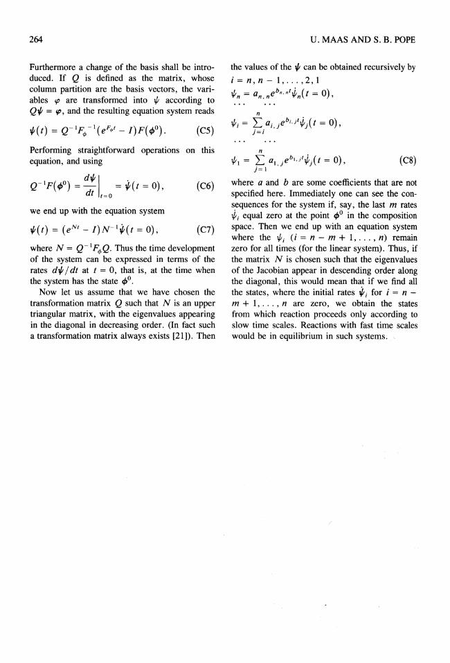
264

Furthermore a change of the basis shall be intro­duced. If Q is defined as the matrix, whose column partition are the basis vectors, the vari­ables cp are transformed into ~ according to Q~ = cp, and the resulting equation system reads

Performing straightforward operations on this equation, and using

d~1 . Q- 1p(4)0)=_ =~(t=O), dt 1=0

(C6)

we end up with the equation system

~(t) = (e N1 - I)N-11f(t = 0), (C7)

where N = Q- I Pq, Q. Thus the time development of the system can be expressed in terms of the rates d~ / dt at t = 0, that is, at the time when the system has the state 4>0.

Now let us assume that we have chosen the transformation matrix Q such that N is an upper triangular matrix, with the eigenvalues appearing in the diagonal in decreasing order. (In fact such a transformation matrix always exists [21]). Then

U. MAAS AND S. B. POPE

the values of the ~ can be obtained recursively by

i=n,n-1, ... ,2,1 .f, = a ebn . nl .;, (t = 0) ¥In n, n YIn ,

n

~i = L ai,jebij~At = 0), }=i

n

~I = L aI,jebl,jl~j(t = 0), }=l

(C8)

where a and b are some coefficients that are not specified here. Immediately one can see the con­sequences for the system if, say, the last m rates ~i equal zero at the point 4>0 in the composition space. Then we end up with an equation system where the ~i (i = n - m + 1, ... , n) remain zero for all times (for the linear system). Thus, if the matrix N is chosen such that the eigenvalues of the Jacobian appear in descending order along the diagonal, this would mean that if we find all the states, where the initial rates Ifi for i = n -m + 1, ... , n are zero, we obtain the states from which reaction proceeds only according to slow time scales. Reactions with fast time scales would be in equilibrium in such systems.