Simplifying proofs of linearisability using layers of abstraction

Brijesh Dongol and John Derrick

Department of Computer Science

The University of Sheffield, S1 4DP, UK

B.Dongol@sheffield.ac.uk, J.Derrick@dcs.shef.ac.uk

Abstract

Linearisability has become the standard correctness criterion for concurrent data structures, ensuring that ev-ery history of invocations and responses of concurrent operations has a matching sequential history. Existingproofs of linearisability require one to identify so-called linearisation points within the operations under con-sideration, which are atomic statements whose execution causes the effect of an operation to be felt. However,identification of linearisation points is a non-trivial task, requiring a high degree of expertise. For sophisticatedalgorithms such as Heller et al’s lazy set, it even is possible for an operation to be linearised by the concurrentexecution of a statement outside the operation being verified. This paper proposes an alternative method for ver-ifying linearisability that does not require identification of linearisation points. Instead, using an interval-basedlogic, we show that every behaviour of each concrete operation over any interval is a possible behaviour of a cor-responding abstraction that executes with coarse-grained atomicity. This approach is applied to Heller et al’s lazyset to show that verification of linearisability is possible without having to consider linearisation points within theprogram code.

1 IntroductionDevelopment of correct fine-grained concurrent data structures has received an increasing amount of attention overthe past few years as the popularity of multi/many-core architectures has increased. An important correctnesscriterion for such data structures is linearisability [16], which guarantees that every history of invocations andresponses of the concurrent operations on the data structure can be rearranged without violating the ordering withina process such that the rearranged history is a valid sequential history. A number of proof techniques developedover the years match concurrent and sequential histories by identifying an atomic linearising statement within theconcrete code of each operation, whose execution corresponds to the effect of the operation taking place. However,due to the subtlety and complexity of concurrent data structures, identification of linearising statements within theconcrete code is a non-trivial task, and it is even possible for an operation to be linearised by the execution ofother concurrent operations. An example of such behaviour occurs in Heller et al’s lazy set algorithm, whichimplements a set as a sorted linked list [15] (see Fig. 1). In particular, its contains operation may be linearisedby the execution of a concurrent add or remove operation and the precise location of the linearisation point isdependent on how much of the list has been traversed by the contains operation. This paper presents a methodfor simplifying proofs of linearisability using Heller et al’s lazy set as an example.

An early attempt at verifying linearisability of Heller et al’s lazy set is that of Vafeiadis et al, who extendeach linearising statement with code corresponding to the execution of the abstract operation so that execution ofa linearising statement causes the corresponding abstract operation to be executed [24]. However, this techniqueis incomplete and cannot be used to verify the contains operation, and hence, its correctness is only treatedinformally [24]. These difficulties reappear in more recent techniques: “In [Heller et al’s lazy set] algorithm, thecorrect abstraction map lies outside of the abstract domain of our implementation and, hence, was not found.”[23]. The first complete linearisability proof of the lazy set was given by Colvin et al [4], who map the concreteprogram to an abstract set representation using simulation to prove data refinement. To verify the contains

1

arX

iv:1

307.

6958

v1 [

cs.L

O]

26

Jul 2

013

operation, a combination of forwards and backwards simulation is used, which involves the development of anintermediate program IP such that there is a backwards simulation from the abstract representation to IP, and aforwards simulation from IP to the concrete program. More recently, O’Hearn et al use a so-called hindsightlemma (related to backwards simulation) to verify a variant of Heller’s lazy set algorithm [20]. Derrick et al use amethod based on non-atomic refinement, which allows a single atomic step of the concrete program to be mappedto several steps of the abstract [6].

Application of the proof methods in [24, 4, 20, 6] remains difficult because one must acquire a high degree ofexpertise of the program being verified to correctly identify its linearising statements. For complicated proofs, it isdifficult to determine whether the implementation is erroneous or the linearising statements have been incorrectlychosen. Hence, we propose an approach that eliminates the need for identification of linearising statements inthe concrete code by establishing a refinement between the fine-grained implementation and an abstraction thatexecutes with coarse-grained atomicity [8]. The idea of mapping fine-grained programs to a coarse-grained ab-straction has been proposed by Groves [13] and separately Elmas et al [12], where the refinements are justifiedusing reduction [18]. However, unlike our approach, their methods must consider each pair of interleavings, andhence, are not compositional. Turon and Wand present a method of abstraction in a compositional rely/guaranteeframework with separation logic [21], but only verify a stack algorithm that does not require backwards reasoning.

Capturing the behaviour of a program over its interval of execution is crucial to proving linearisability ofconcurrent data structures. In fact, as Colvin et al point out: “The key to proving that [Heller et al’s] lazy set islinearisable is to show that, for any failed contains(x) operation, x is absent from the set at some point during itsexecution.” [4]. Hence, it seems counter-intuitive to use logics that are only able to refer to the pre and post statesof each statement (as done in [24, 4, 6, 23]). Instead, we use a framework based on [9] that allows reasoning aboutthe fine-grained atomicity of pointer-based programs over their intervals of execution. By considering completeintervals, i.e., those that cover both the invocation and response of an operation, one is able to determine the futurebehaviour of a program, and hence, backwards reasoning can often be avoided. For example, Bäumler et al [2] usean interval-based approach to verify a lock-free queue without resorting to backwards reasoning, as is required byframeworks that only consider the pre/post states of a statement [7]. However, unlike our approach, Bäumler et almust identify the linearising statements in the concrete program, which is a non-trivial step.

An important difference between our framework and those mentioned above is that we assume a truly con-current execution model and only require interleaving for conflicting memory accesses [8, 9]. Each of the otherframeworks mentioned above assume a strict interleaving between program statements. Thus, our approach cap-tures the behaviour of program in a multicore/multiprocesor architecture more faithfully.

The main contribution of this paper is the use of the techniques in [8] to simplify verification of a complex setalgorithm by Heller et al. This algorithm presents a challenge for linearisability because the linearisation point ofthe contains operation is potentially outside the operation itself [6]. We propose a method in which the proof issplit into several layers of abstraction so that linearisation points of the fine-grained implementation need not beidentified. As summarised in Fig. 3, one must additionally prove that the coarse-grained abstraction is linearisable,however, due to the coarse granularity of atomicity, the linearising statements are straightforward to identify andthe linearisability proof itself is simpler [8]. Other contributions of this paper include a method for reasoningabout truly concurrent program executions and an extension of the framework in [9] to enable reasoning aboutpointer-based programs, which includes methods for reasoning about expressions non-deterministically [14].

2 A list-based concurrent setHeller et al [15] implement a set as a concurrent algorithm operating on a shared data structure (see Fig. 1) withoperations add and remove to insert and delete elements from the set, and an operation contains to checkwhether an element is in the set. The concurrent implementation uses a shared linked list of node objects withfields val, nxt,mrk, and lck, where val stores the value of the node, nxt is a pointer to the next node in the list, mrkdenotes the marked bit and lck stores the identifier of the process that currently holds the lock to the node (if any)[15]. The list is sorted in strictly ascending values order (including marked nodes).

Operation locate(x) is used to obtain pointers to two nodes whose values may be used to determine whetheror not x is in the list — the value of the predecessor node pred must always be less than x, and the value of the

2

add(x):A1: n1, n3:=

locate(x);A2: if n3.val != xA3: n2:=

new Node(x);A4: n2.nxt := n3;A5: n1.nxt := n2;A6: res := trueA7: else res := false

endif;A8: n1.unlock();A9: n3.unlock();A10: return res

remove(x):R1: n1, n2 :=

locate(x);R2: if n2.val = xR3: n2.mrk := true;R4: n3 := n2.nxt;R5: n1.nxt := n3;R6: res := trueR7: else res := false

endif;R8: n1.unlock();R9: n2.unlock();R10: return res

contains(x):C1: n1 := Head;C2: while (n1.val < x)C3: n1 := n1.nxt

enddo;C4: res := (n1.val = x)

and !n1.mrkC5: return res

locate(x):while (true) do

L1: pred := Head;L2: curr := pred.nxt;L3: while (curr.val < x) doL4: pred := curr;L5: curr := pred.nxt enddo;L6: pred.lock();

L7: curr.lock();L8: if !pred.mrk and !curr.mrk

and pred.nxt = currL9: return pred, currL10: else pred.unlock();L11: curr.unlock() endif enddo

Figure 1: Heller et al’s lazy set algorithm

∆uadd(x)

∆′q

add(y)remove(x)∆q

LazySet∆s

∆pcontains(x)

vC1 (C2 ; C3)ω C4 return true

return true〈x ∈ absSet〉

Figure 2: Execution of contains(x) over ∆p that returns true

Abstract sequential program

Behaviour refinement

Fine-grained implementation

Coarse-grained abstraction

Linearisability proof

Figure 3: Proof steps

current node curr may either be greater than x (if x is not in the list) or equal to x (if x is in the list). Operationadd(x) calls locate(x), then if x is not already in the list (i.e., value of the current node n3 is strictly greaterthan x), a new node n2 with value field x is inserted into the list between n1 and n3 and true is returned. If xis already in the list, the add(x) operation does nothing and returns false. Operation remove(x) also starts bycalling locate(x), then if x is in the list the current node n2 is removed and true is returned to indicate thatx was found and removed. If x is not in the list, the remove operation does nothing and returns false. Notethat operation remove(x) distinguishes between a logical removal, which sets the marked field of n2 (the nodecorresponding to x), and a physical removal, which updates the nxt field of n1 so that n2 is no longer reachable.Operation contains(x) iterates through the list and if a node with value greater or equal to x is found, it returnstrue if the node is unmarked and its value is equal to x, otherwise returns false.

The complete specification consists of a number of processes, each of which may execute its operation on theshared data structure. For the concrete implementation, therefore, the set operations can be executed concurrentlyby a number of processes, and hence, the intervals in which the different operations execute may overlap. Our basicsemantic model uses interval predicates (see Section 3), which allows formalisation of a program’s behaviour withrespect to an interval (which is a contiguous set of times), and an infinite stream (that maps each time to a state).

3

For example, consider Fig. 2, which depicts an execution of the lazy set over interval ∆ in stream s, a process pthat executes a contains(x) that returns true over ∆p, a process q that executes remove(x) and add(y) overintervals ∆q and ∆′

q, respectively, and a process u that executes add(x) over interval ∆u. Hence, the shared datastructure may be changing over ∆p while process p is checking to see whether x is in the set.

Correctness of such concurrent executions is judged with respect to linearisability, the crux of which re-quires the existence of an atomic linearisation point within each interval of an operation’s execution, corre-sponding to the point at which the effect of the operation takes place [16]. The ordering of linearisation pointsdefines a sequential ordering of the concurrent operations and linearisability requires that this sequential order-ing is valid with respect to the data structure being implemented. For the execution in Fig. 2, assuming thatthe set is initially empty, because contains(x) returns true, a valid linearisation corresponds to a sequen-tial execution Seq1 “= add(x); contains(x); remove(x); add(y) obtained by picking linearisation pointswithin ∆u, ∆p, ∆q and ∆′

q in order. Note that a single concurrent history may be linearised by more thanone valid sequential history, e.g., the execution in Fig. 2 can correspond to the sequential execution Seq2 “=remove(x); add(x); contains(x); add(y). The abstract sets after completion of Seq1 and Seq2 are yand x, y, respectively. Unlike Seq1, operation remove(x) in Seq2 returns false. Note that a linearisation of ∆′

qcannot occur before ∆q because remove(x) responds before the invocation of add(y).

Herlihy and Wing formalise linearisability in terms of histories of invocation and response events of the op-erations on the data structure in question [16]. Clearly, reasoning about such histories directly is infeasible, andhence, existing methods (e.g., [4, 6, 24]) prove linearisability by identifying an atomic linearising statement withinthe operation being verified and showing that this statement can be mapped to the execution of a corresponding ab-stract operation. However, due to the fine granularity of the atomicity and inherent non-determinism of concurrentalgorithms, identification of such a statement is difficult. The linearising statement for some operations may actu-ally be outside the operation, e.g., none of the statements C1-C5 are valid linearising statements of contains(x);instead contains(x) is linearised by the execution of a statement within add(x) or remove(x) [6].

As summarised in Fig. 3, we decompose proofs of linearisability into two steps, the first of which provesthat a fine-grained implementation refines a program that executes the same operations but with coarse-grainedatomicity. The second step of the proof is to show that the abstraction is linearisable. The atomicity of a coarse-grained abstraction cannot be guaranteed in hardware (without the use of contention inducing locks), however,its linearisability proof is much simpler [9]. Because we prove behaviour refinement, any behaviour of the fine-grained implementation is a possible behaviour of the coarse-grained abstraction, and hence, an implementation islinearisable whenever the abstraction is linearisable. Our technique does not require identification of the linearisingstatements in the implementation.

A possible coarse-grained abstraction of contains(x) is an operation that is able to test whether x is in theset in a single atomic step (see Fig. 6), unlike the implementation in Fig. 1, which uses a sequence of atomicsteps to iterate through the list to search for a node with value x. Therefore, as depicted in Fig. 2, an execution ofcontains that returns true, i.e., C1 ; (C2 ; C3)ω ; C4 ; return true, is required to refine a coarse-grained abstraction〈x ∈ absSet〉 ; return true, where C1 - C4 are the labels of contains in Fig. 1 and 〈x ∈ absSet〉 is a guard thatis atomically able to test whether x is in the abstract set. In particular, 〈x ∈ absSet〉 holds in an interval Ω andstream s iff there is a time t in Ω such that x ∈ absSet.(s.t). Streams are formalised in Section 3. Note that both〈x ∈ absSet〉 and 〈x 6∈ absSet〉may hold within ∆p; the refinement in Fig. 2 would only be invalid if for all t ∈ ∆p,x 6∈ absSet.(s.t) holds.

Proving refinement between a coarse-grained abstraction and an implementation is non-trivial due to the exe-cution of other (interfering) concurrent processes. Furthermore, our execution model allows non-conflicting state-ments (e.g., concurrent writes to different locations) to be executed in a truly concurrent manner. We use composi-tional rely/guarantee-style reasoning [17] to formalise the behaviour of the environment of a process and allow theexecution of an arbitrary number of processes in the environment. Note that unlike Jones [17], who assumes relyconditions are two-state relations, rely conditions in our framework are interval predicates that are able to refer toan arbitrary number of states.

4

CLoop(p, x) = ([(n1p 7→ val) < x] ; n1p := (n1p 7→ nxt))ω ; [(n1p 7→ val) ≥ x]Contains(p, x) = cl1: n1p := Head ; cl2:CLoop(p, x) ;

cl3: resp := (¬(n1p 7→ mrk) ∧ (n1p 7→ val) = x)

HTInit = (Head 7−→ (−∞, Tail, false, null)) ∧ (Tail 7−→ (∞, null, false, null))

S(p) = Jn1p, n2p, n3p, resp (d

x:Z Add(p, x) u Remove(p, x) u Contains(p, x))ωK

Set(P) = JHead, Tail RELY←−−−HTInit • ‖p:P S(p)K

Figure 4: Formal model of the lazy set operations

3 Interval-based frameworkTo simplify reasoning about the linked list structure of the lazy list, the domain of each state distinguishes betweenvariables and addresses. We use a language with an abstract syntax that closely resembles program code, and useinterval predicates to formalise interval-based behaviour. Fractional permissions are used to control conflictingaccesses to shared locations.

Commands. We assume variable names are taken from the set Var, values have type Val, addresses have typeAddr “= N, Var ∩ Addr = ∅ and Addr ⊆ Val. A state over VA ⊆ Var ∪ Addr has type StateVA “= VA → Val and astate predicate has type StateVA → B.

The objects of a data structure may contain fields, which we assume are of type Field. We assume that everyobject with m fields is assigned m contiguous blocks of memory and use offset: Field → N to obtain the offset off ∈ Field within this block [22], e.g., for the fields of a node object, we assume that offset.val = 0, offset.nxt = 1,offset.mrk = 2 and offset.lck = 3.

We assume the existence of a function eval that evaluates a given expression in a given state. The full detailsof expression evaluation are elided. To simplify modelling of pointer-based programs, for an address-valued ex-pression ae, we introduce expressions ∗ ae, which returns the value at address ae, ae·f , which returns the addressof f with respect to ae. For a state σ, we define eval.(∗ ae).σ “= σ.(eval.ae.σ) and (ae·f ).σ “= eval.ae.σ + offset.f .We also define shorthand ae 7→ f “= ∗(ae·f ), which returns the value at ae·f in state σ.

Assuming that Proc denotes the set of process ids, for a set of variables Z, state predicate c, variable or address-valued expression vae, expression e, label l, and set of processes P ⊆ Proc, the abstract syntax of a command isgiven by Cmd below, where C,C1,C2,Cp ∈ Cmd.

Cmd ::= Idle | [c] | 〈c〉 | vae := e | C1 ; C2 | C1 u C2 | Cω | ‖p:P Cp | JZ CK | l: C

Hence a command is either Idle, a guard [c], an atomically evaluated guard 〈c〉, an assignment vae := e, a sequentialcomposition C1 ; C2, a non-deterministic choice C1 u C2, a possibly infinite iteration Cω , a parallel composition‖p:P Cp, a command C within a context Z (denotedJZ CK), or a labelled command l: C.

A formalisation of part of Heller et al’s lazy list using the syntax above is given in Fig. 4, where P ⊆ Proc.Operations add(x), remove(x) and contains(x) executed by process p are modelled by commands Add(p, x),Remove(p, x) and Contains(p, x), respectively. We assume that n 7−→ (vv, nn,mm, ll) denotes (n 7→ val = vv) ∧(n 7→ nxt = nn) ∧ (n 7→ mrk = mm) ∧ (n 7→ lck = ll). Details of Add(p, x) and Remove(p, x) are elided andthe RELY construct is formalised in Section 5.1 Note that unlike the methods in [4, 6], where labels identify theatomicity, we use labels to simplify formalisation of the rely conditions of each process, and may correspond toa number of atomic steps. Furthermore, guard evaluation is formalised with respect to the set of states apparentto a process (see Section 4), and hence, unlike [24, 4, 6], we need not split complex expressions into their atomiccomponents. For example, in [24, 4, 6], the expression at C4 (Fig. 1) must be split into two expressions curr.val= x and !curr.mrk to explicitly model the fact that interference may occur between accesses to curr.val andcurr.mrk.

1The formalisation is given in Appendix A.

5

Interval predicates. A (discrete) interval (of type Intv) is a contiguous set of time (of type Time “= Z), i.e.,Intv “= ∆ ⊆ Time | ∀t, t′: ∆ • ∀u: Time • t ≤ u ≤ t′ ⇒ u ∈ ∆. Using ‘.’ for function application, we let lub.∆and glb.∆ denote the least upper and greatest lower bounds of an interval ∆, respectively, where lub.∅ “= −∞and glb.∅ “= ∞. We define inf.∆ “= (lub.∆ = ∞), fin.∆ “= ¬inf.∆ and empty.∆ “= (∆ = ∅). For a set K andi, j ∈ K, we let [i, j]K “= k: K | i ≤ k ≤ j denote the closed interval from i to j containing elements from K. Onemust often reason about two adjoining intervals, i.e., intervals that immediately precede or follow a given interval.We say ∆ adjoins ∆′ iff ∆∝∆′, where

∆∝∆′ “= (∀t: ∆, t′: ∆′ • t < t′) ∧ (∆ ∪∆′ ∈ Intv)

Note that adjoining intervals ∆ and ∆′ must be disjoint, and by conjunct ∆ ∪∆′ ∈ Intv, the union of ∆ and ∆′

must be contiguous. Note that both ∆∝∅ and ∅∝∆ hold trivially for any interval ∆.A stream of behaviours over VA ⊆ Var∪Addr is given by a total function of type StreamVA “= Time→ StateVA,

which maps each time to a state over VA. To reason about specific portions of a stream, we use interval predicates,which have type IntvPredVA “= Intv → StreamVA → B. Note that because a stream encodes the behaviour over alltime, interval predicates may be used to refer to the states outside a given interval. Like Interval Temporal Logic[19], we may define a number of operators on interval predicates. For example, if g ∈ IntvPredVA, ∆ ∈ Intv ands ∈ StreamVA, we define:

(g).∆.s “= ∀∆′: Intv • ∆′ ⊆ ∆⇒ g.∆′.s (g).∆.s “= ∃∆′ • ∆′ ∝∆ ∧ g.∆′.s

We assume pointwise lifting of operators on stream and interval predicates in the normal manner, define universalimplication g1 V g2 “= ∀∆: Intv, s: Stream • g1.∆.s ⇒ g2.∆.s for interval predicates g1 and g2, and say g1 ≡ g2

holds iff both g1 V g2 and g2 V g1 hold.We define two operators on interval predicates: chop, which is used to formalise sequential composition, and

ω-iteration, which is used to formalise a possibly infinite iteration (e.g., a while loop). The chop operator ‘;’ is abasic operator on two interval predicates [19, 9, 10], where (g1 ; g2).∆ holds iff either interval ∆ may be split intotwo parts so that g1 holds in the first and g2 holds in the second, or the least upper bound of ∆ is∞ and g1 holdsin ∆. The latter disjunct allows g1 to formalise an execution that does not terminate. Using chop, we define thepossibly infinite iteration (denoted gω) of an interval predicate g as the greatest fixed point of z = (g ; z) ∨ empty,where the interval predicates are ordered using ‘V’ (see [11] for details). We define

(g1 ; g2).∆.s “= Å∃∆1,∆2: Intv • (∆ = ∆1 ∪∆2) ∧

(∆1 ∝∆2) ∧ g1.∆1.s ∧ g2.∆2.s

ã∨ (inf ∧ g1).∆.s

gω “= νz • (g ; z) ∨ empty

In the definition of g1 ; g2, interval ∆1 may be empty, in which case ∆2 = ∆, and similarly ∆2 may empty, inwhich case ∆1 = ∆. Hence, both (empty ; g) ≡ g and g ≡ (g ; empty) trivially hold. An iteration gω of g mayiterate g a finite (including zero) number of times, but also allows an infinite number of iterations [11].

Permissions and interference. To model true concurrency, the behaviour of the parallel composition betweentwo processes in an interval ∆ is modelled by the conjunction of the behaviours of both processes executing within∆. Because this potentially allows conflicting accesses to shared variables, we incorporate fractional permissionsinto our framework [3, 9]. We assume the existence of a permission variable in every state σ ∈ StateVA oftype VA → Proc → [0, 1]Q, where VA ⊆ Var ∪ Addr and Q denotes the set of rationals. A process p ∈ Prochas write-permission to location va ∈ VA in σ ∈ StateVA iff σ.Π.va.p = 1; has read-permission to va in σ iff0 < σ.Π.va.p < 1; and has no-permission to access va in σ iff σ.Π.va.p = 0.

We defineR.va.p.σ “= (0 < σ.Π.va.p < 1) andW.va.p.σ “= (σ.Π.va.p = 1) and D.va.p.σ “= (σ.Π.va.p = 0)to be state predicates on permissions. In the context of a stream s, for any time t ∈ Z, process p may only writeto and read from va in the transition step from s.(t − 1) to s.t ifW.va.p.(s.t) and R.va.p.(s.t) hold, respectively.Thus, W.va.p.(s.t) does not give p permission to write to va in the transition from s.t to s.(t + 1) (and similarlyR.va.p). For example, to state that process p updates variable v to value k at time t of stream s, the effect of theupdate should imply ((v = k) ∧ W.v.p).(s.t).

6

One may introduce healthiness conditions on streams that formalise our assumptions on the underlying hard-ware. We assume that at most one process has write permission to a location va at any time, which is guaranteedby ensuring the sum of the permissions of the processes on va at all times is at most 1, i.e.,

∀s: Stream, t: Time • ((Σp∈ProcΠ.va.p) ≤ 1).(s.t)

Other conditions may be introduced to model further restrictions as required [9].Fractional permissions may also be used to characterise interference within a process p. For a set of variables,

we define I.VA.p “= ∃v: VA • ∃q: Proc\p •W.v.q. Such notions are particularly useful because we aim to developrely/guarantee-style reasoning, where we use rely conditions to characterise the behaviour of the environment. Onemay introduce rely conditions that refer to I.VA.p to characterise the interference on VA by the environment of p.

4 Evaluating state predicates over intervalsThe set of times within an interval corresponds to a set of states with respect to a given stream. Hence, if oneassumes that expression evaluation is non-atomic (i.e., takes time), one must consider evaluation with respect to aset of states, as opposed to a single state. It turns out that there are a number of possible ways in which such anevaluation can take place, with varying degrees of non-determinism [14]. In this paper, we consider actual statesevaluation, which evaluates an expression with respect to the set of actual states that occur within an interval andapparent states evaluation, which considers the set of states apparent to a given process.

Actual states evaluation allow one to reason about the true state of a system, and evaluates an expressioninstantaneously at a single point in time. However, a process executing with fine-grained atomicity can only reada single variable at a time, and hence, will seldom be able to view an actual state because interference may occurbetween two successive reads. For example, a process p evaluating ecl3 (the expression at cl3) cannot read bothn1p 7→ mrk and n1p 7→ val in a single atomic step, and hence, may obtain a value for ecl3 that is different fromany actual value of ecl3 because interference may occur between reads to n1p 7→ mrk and n1p 7→ val. Therefore,we define an apparent states evaluator that models fine-grained expression evaluation over intervals. Our definitionof apparent states evaluation does not fix the order in which n1p 7→ mrk and n1p 7→ val are read. We see this asadvantageous over frameworks that must make the atomicity explicit (e.g., [24, 4, 6]), which require an orderingto be chosen, even if an evaluation order is not specified by the corresponding implementation (e.g., [15]). In[24, 4, 6], if the order of evaluation is modified, the linearisability proof must be redone, whereas our proof is moregeneral because it shows that any order of evaluation is valid.Evaluation over actual states. To formalise evaluators over actual states, for an interval ∆ and stream s ∈StreamVA, we define states.∆.s “= σ: StateVA | ∃t: ∆ • σ = s.t. Two useful operators for a sets of actual statesof a state predicate c are c and c, which specify that c holds in some and all actual state of the given streamwithin the given interval, respectively.

( c).∆.s “= ∃σ: states.∆.s • c.σ (c).∆.s “= ∀σ: states.∆.s • c.σ

Example 4.1. Suppose v is a variable, fa and fb are fields, and s is a stream such that the expression (v 7→fa, v 7→ fb) always evaluates to (0, 0), (1, 0) and (1, 1) within intervals [1, 4]N, [5, 10]N and [11, 16]N, respectively,i.e., for example ((v 7→ fa, v 7→ fb) = (0, 0)).[1, 4]N.s. Thus, both ((v 7→ fa) ≥ (v 7→ fb)).[1, 16]N.s and((v 7→ fa) > (v 7→ fb)).[1, 16]N.s may be deduced.

Using, we define←−c and−→c , which hold iff c holds at the beginning and end of the given interval, respectively.

←−c .∆.s “= (c ∧ ¬empty) ; true −→c .∆.s “= true ; (c ∧ ¬empty)

Operators and cannot accurately model fine-grained interleaving in which processes are able to access atmost one location in a single atomic step. However, both and are useful for modelling the actual behaviourof the system as well as the behaviour of the coarse-grained abstractions that we develop. We may use to definestability of a variable v, and invariance of a state predicate c as follows:

stable.v “= ∃k • −−−−−→(va = k) ∧ (va = k) inv.c “= −→c ⇒ c

7

Such definitions of stability and invariance are necessary because adjoining intervals are assumed to be disjoint,i.e., do not share a point of overlap. Therefore, one must refer to the values at the end of some immediatelypreceding interval.Evaluation over states apparent to a process. Assuming the same setup as Example 4.1, if p is only able toaccess at most one location at a time, evaluating (v 7→ fa) < (v 7→ fb) using the states apparent to process p overthe interval [1, 16]N may result in true, e.g., if the value at v·fa is read within interval [1, 4]N and the value at v·fbread within [11, 16]N.

Reasoning about the apparent states with respect to a process p using function apparent is not always adequatebecause it is not enough for an apparent state to exist; process p must also be able to read the relevant variablesin this apparent state. Typically, it is not necessary for a process to be able to read all of the state variablesto determine the apparent value of a given state predicate. In fact, in the presence of local variables (of otherprocesses), it will be impossible for p to read the value of each variable. Hence, we define a function apparentp,W ,where W ⊆ Var∪Addr is the set of locations whose values process p needs to determine to evaluate the given statepredicate.

apparentp,W .∆.s “= σ: StateW | ∀ va: W • ∃t: ∆ • (σ.va = s.t.va) ∧ R.va.p.(s.t)

Using this function, we are able to determine whether state predicates definitely and possibly hold with respect theapparent states of a process. For a state predicate c, interval ∆, stream s and state σ, we let accessed.c.σ denotethe smallest set of locations (variables and addresses) that must be accessed in order to evaluate c in state σ anddefine locs.c.∆.s “= ⋃

t∈∆ accessed.c.(s.t). For a process p, this is used to define (p c).∆.s, which states that cholds in all states apparent to p in s within ∆. (Similarly ( p c).∆.s.)

(p c).∆.s “= let W = locs.c.∆.s in ∀σ: apparentp,W .∆.s • c.σ( p c).∆.s “= let W = locs.c.∆.s in ∃σ: apparentp,W .∆.s • c.σ

Continuing Example 4.1, if c “= ((v 7→ fa) ≥ (v 7→ fb)), we have (¬p c).[1, 16]N.s holds, i.e., ( p ¬c).[1, 16]N.seven though (c).[1, 16]N.s holds (cf. [9, 14]). One may establish a number of properties on , , and [14],for example p(c ∧ d)V pc ∧ pd holds. The following lemma relates apparent and states evaluation.

Lemma 1. For any process p, variable v, field f and constant k,stable.v ∧ p((v 7→ f ) = k)⇒ ((v 7→ f ) = k)

5 Behaviours and refinementThe behaviour of a command C executed by a non-empty set of processes P in a context Z ⊆ Var is given byinterval predicate behP,Z .C, which is defined inductively in Fig. 5. We use behp,Z to denote behp,Z and assumethe existence of a program counter variable pcp for each process p. We define shorthand fin Idle “= ENF fin • Idleand inf Idle “= ENF inf • Idle to denote finite and infinite idling, respectively and use the interval predicates belowto formalise the semantics of the commands in Fig. 5.

evalp,Z .c “= p c ∧ behp,Z .Idle

updatep,Z(va, k) “= ßbehp,Z\va.Idle ∧ ¬empty ∧ (va = k ∧ Wp.va) if va ∈ Varbehp,Z\va.Idle ∧ ¬empty ∧ ((∗va) = k ∧ Wp.va) if va ∈ Addr

To enable compositional reasoning, for interval predicates r and g, and command C, we introduce two additionalconstructs RELY r • C and ENF g • C, which denote a command C with a rely condition r and an enforced conditiong, respectively [9].

We say that a concrete command C is a refinement of an abstract command A iff every possible behaviour of Cis a possible behaviour of A. Command C may use additional variables to those in A, hence, we define refinementin terms of sets of variables corresponding to the contexts of A and C. In particular, we say A with context Y isrefined by C with context Z with respect to a set of processes P (denoted A vY,Z

P C) iff behP,Z .CV behP,Y .A holds.Thus, any behaviour of the concrete command C is a possible behaviour of the abstract command A. This is akin to

8

behp,Z .Idle = ∀va: Z • ¬W.va.pbehp,Z .[c] = p c ∧ behp,Z .Idlebehp,Z .〈c〉 = c ∧ behp,Z .IdlebehP,Z .Cω = (behP,Z .C)ω

behp,Z .(l:C) = (pcp = l) ∧ behp,Z .C

behP,Z .(C1 ; C2) = behP,Z .C1 ; behP,Z .C2

behP,Z .(C1 u C2) = behP,Z .C1 ∨ behP,Z .C2

behP,Z .(RELY r • C) = r ⇒ behP,Z .CbehP,Z .(ENF g • C) = g ∧ behP,Z .C

behp,Z .(vae := e) =

ß∃k • evalp,Z .(e = k) ; updatep,Z(v, k) if vae ∈ Var∃k, a • evalp,Z .(vae = a ∧ e = k) ; updatep,Z(a, k) otherwise

behP,Z .(‖p:P Cp) =

true if P = ∅behp,Z .Cp if P = p∃P1,P2, S1, S2

• (P1 ∪ P2 = P) ∧ (P1 ∩ P2 = ∅) ∧ P1 6= ∅ ∧ P2 6= ∅ ∧S1 ∈ fin Idle, inf Idle ∧ S2 ∈ fin Idle, inf Idle ∧(S1 = inf Idle⇒ S2 6= inf Idle) ∧behP1,Z .((‖p:P1

Cp) ; S1) ∧ behP2,Z .((‖p:P2Cp) ; S2)

otherwise

behP,Z .JY CK = (Z ∩ Y = ∅) ∧ behP,Z∪Y .C

Figure 5: Formalisation of behaviour function

operation refinement [5], however, our definition is with respect to the intervals over which the commands execute,as opposed to their pre/post states. We write A vZ

P C for A vZ,ZP C, write A vP C for A v∅

P C, write A vwZP C

iff both A vZP C and C vZ

P A, and write A vY,Zp C for A vY,Z

p C. There are numerous theorems and lemmas forbehaviour refinement [9, 8]. We present a selection of results that are used to verify correctness of the lazy set.The following results may be proved using monotonicity of the corresponding interval predicate operators.

The next lemma states that an assignment of state predicate c to a variable v may be decomposed to a guard [c]followed by an assignment of true to v and a guard [¬c] followed by an assignment of false to v.

Lemma 2. For a state predicate c, variable v, process p, and Z ⊆ Var ∪ Addr, we havev := c vZ

p ([c] ; v := true) u ([¬c] ; v := false).

Note that a property like Lemma 2 is difficult to formalise in interleaved frameworks such as action systems[1] because interference may occur between guard evaluation and assignment to v at the concrete level, which isnot possible in the abstract. The lemma below allows one to move the frame of a command into the refinementrelation.

Lemma 3. Suppose A and C are commands, P ⊆ Proc, W,X ⊆ Var and Y,Z ⊆ Var∪Addr such that W ⊆ (X∪Z)and W ∩ Y = ∅ = X ∩ Z. If A vW∪Y,X∪Z

P C, thenJW AK vY,ZP JX CK.

The following theorem allows one to turn a rely condition at the abstract level to an enforced condition at theconcrete level, establishing a Galois connection between rely and enforced conditions [9].

Theorem 5.1. (RELY r • A) vY,ZP C ⇔ A vY,Z

P (ENF r • C)

When modelling a lock-free algorithm [4, 6, 24], one assumes that each process repeatedly executes operationsof the data structure, and hence the processes of the system only differ in terms of the process ids. For suchprograms, a proof of the parallel composition may be decomposed using the following theorem [8].

Theorem 5.2. If p ∈ Proc, Y,Z ⊆ Var ∪ Addr, and A(p) and C(p) are commands parameterised by p, then(RELY g • ‖p:P A(p)) vY,Z

P (‖p:P C(p)) holds if for some interval predicate r and some p ∈ P and Q “= P\p bothof the following hold.

RELY g ∧ r • A(p) vY,Zp C(p) (1)

g ∧ behQ,Z .(‖q:Q C(q)) V r (2)

9

ϕk+1.ua.σ = if(k = 0) then ua else eval.((ϕk.ua.σ) 7→ nxt).σRE.ua.vb.σ = ∃k:N • ϕk.ua.σ = vb

setAddr.σ =

a:Addr RE.Head.a.σ ∧ ¬eval.(a 7→ mrk).σ

absSet.σ =

v:Val ∃a: setAddr.σ • v = eval.(a 7→ val).σ

CGCon(p, x) = (〈x ∈ absSet〉 ; resp := true) u (〈x 6∈ absSet〉 ; resp := false)

CGS(p) = Jresp(d

x:Z

(Jn1p, n2p, n3p Add(p, x) u Remove(p, x)K u CGCon(p, x)

))ωKCGSet(P) = JHead, Tail RELY

←−−−HTInit • ‖p:P CGS(p)K

Figure 6: A coarse-grained abstraction of contains

RELY r •CGS(p)vHT

pS(p)

vL,Mp

RELY r • Add(p, x) u Remove(p, x)Lemma 3

Add(p, x) u Remove(p, x)

RELY r •CGCon(p, x)vL,M

pContains(p, x)

Theorem 5.2Lemma 3

Set(P)vP

CGSet(P)

behQ,HT .(‖q:Q S(q))V r

Figure 7: Proof decomposition for the lazy set verification

6 Verification of the lazy setAs already mentioned, we focus on a proof contains, which highlights the advantages of interval-based reasoningover frameworks that only reason about the pre/post states.2 Verification of linearisability of contains is knownto be difficult using frameworks that only consider the pre/post states [23, 24, 4, 6]. A coarse-grained abstractionof Set(P) in Fig. 4 is given by CGSet(P) in Fig. 6, where the Add and Remove operations are unmodified, butContains is replaced by CGCon, which tests to see if x is in the set using an atomic (coarse-grained) guard, thenupdates the return value to true or false depending on the outcome of the test.

State predicates reachable, setAddr and absSet, which are used our refinement proof, are defined in Fig. 6.A location vb is reachable from ua in state σ iff RE.ua.vb.σ holds, hence, for example, RE.Head.n.σ holds iffit is possible to traverse the list starting from Head and reach node n in σ. The abstract set of node addressescorresponding to each list data structure in σ is given by setAddr and the set of values of these nodes is given byabsSet.σ. Although null is always reachable from Head, setAddr will not contain null because null 6∈ Addr.

An overview of the proof decomposition is given in Fig. 7. To prove that Set(P) refines CGSet(P), usingTheorem 5.2 we show that S(p) refines CGS(p) for a single process p ∈ P under a yet to be determined relycondition r (condition (1)), provided that the behaviour of the rest of the program implies the r that is derived(condition (2)). Then, using monotonicity of v and Lemma 3, we further decompose the proof that S(p) refinesCGS(p) to the level of each operation. The proofs for Add and Remove are trivial because they are unmodified inCGS(p). To prove Contains, we use Lemma 2 to perform case analysis on executions that return true and false.The refinement proof is hence localised as much as possible. Furthermore, the structure of r is elucidated as partof the correctness proof.

We are required to prove CGSet(P) vP Set(P) for an arbitrarily chosen set of processes P ⊆ Proc. UsingLemma 3, we transfer the context HT “= Addr∪Head,Tail of CGSet(P) and Set(P) into the refinement relation.Then, using monotonicity ofv followed by Theorem 5.2, we decompose the specifications into the following proofobligations, where p ∈ P and Q “= P\p and the rely condition r is yet to be developed.

S1 “= RELY r • CGS(p) vHTp S(p) S2 “= behQ,HT .(‖q:Q S(q))V r

Proof of S1. Using Lemma 3 to expand the context followed by monotonicity of ω and u, assuming L “= HT ∪resp and M “= L ∪ n1p, n2p, n3p, condition S1 decomposes as follows.

RELY r •Jn1p, n2p, n3p(Add(p, x) u Remove(p, x)

)K vL,M

p Add(p, x) u Remove(p, x) (3)

2A verification of the add and remove operations are presented in Appendix A.

10

RELY r • CGCon(p, x) vL,Mp Contains(p, x) (4)

Condition (3) is trivial by Lemma 3 and reflexivity of vMp . To prove (4), must ensure that if resp is assigned

true, then there must have been an actual state, say σ, in the interval preceding the assignment to resp such thatx ∈ setVal.σ. Similarly, if resp is assigned false, there must have been an actual state σ within the interval ofexecution such that x 6∈ setVal.σ. Note that in the proof, we use the states apparent to process p to deduce aproperty of an actual state of the system. Using Lemma 2, Contains(p, x) is equivalent to the following, where

IN “= ¬(n1p 7→ mrk) ∧ ((n1p 7→ val) = x) CL “= cl1: (n1p := Head) ; cl2: CLoop(p, x)

and split the label cl3 into clt3 and clf3 — the true and false cases of IN.

CL ; ((clt3: ([IN] ; resp := true)) u (clf3: ([¬IN] ; resp := false)))

We distribute CL within the ‘u’, use monotonicity to match the abstract and concrete true and false branches, thenuse monotonicity again to remove the assignments to resp from both sides of the refinement. Thus, we are requiredto prove the following properties.

RELY r • 〈x ∈ absSet〉 vL,MP CL ; clt3: [IN] (5)

RELY r • 〈x 6∈ absSet〉 vL,MP CL ; clf3: [¬IN] (6)

Condition (5) (i.e., the branch that assigns resp := true) states that there must be an actual state σ within theinterval in which CL ; clt3: [IN] executes, such that x ∈ absSet.σ holds, which indicates that there is a point atwhich the abstract set contains x. It may be the case that a process q 6= p has removed x from the set by the timeprocess p returns from the contains operation. In fact, x may be added and removed several times by concurrentadd and remove operations before process p completes execution of Contains(p, x). However, this does not affectlinearisability of Contains(p, x) because a state for which x ∈ absSet holds has been found. An execution ofContains(p, x) that returns true would only be incorrect (not linearisable) if true is returned and (x 6∈ absSet)holds for the interval in which CL ; clt3: [IN] executes. Similarly, we prove correctness of (6) by showing that isimpossible for there to be an execution that returns false if (x ∈ absSet) holds in the interval of execution.Proof of (5). Using Theorem 5.1, we transfer the rely condition r to the right hand side as an enforced property.We define state predicate inSet(ua, x), which states that ua with value x is in the abstract set, i.e., inSet(ua, x) “=RE.Head.ua ∧ ¬(ua 7→ mrk) ∧ (ua 7→ val = x). We require that r implies the following.

inv.(RE.Head.n1p ∨ (n1p 7→mrk)) (7)((pcp = cl3)⇒ inv.(n1p 7→ mrk) ∧ ∀k: Val • inv.((n1p 7→ val) = k)) (8)

The behaviour of the right hand side of (5) then simplifies as follows.

behp,M.(ENF r • CL ; cl3: [IN])≡ definition of beh

r ∧ (behp,M.CL ; behp,M.(cl3: [IN]))V definition of beh and n1p is local to p

r ∧ (behp,M.CL ; (stable.n1p ∧ behp,M.(cl3: [IN])))V p(c ∧ d)V p c ∧ p d and Lemma 1

r ∧(behp,M.(cl1: n1p := Head); behp,M.(cl2: CLoop(p, x)); ¬(n1p 7→ mrk) ∧ ((n1p 7→ val) = x)

)V first chop: change context n1p 6∈ L, second chop: assumption (7)

r ∧(behp,L.Idle ; (RE.Head.n1p ∨ (n1p 7→ mrk)) ; ( ¬(n1p 7→ mrk) ∧ ((n1p 7→ val) = x))

)Focusing on just the second and third parts of the chop, because n1p is not modified after CLoop, and r is assumedto split, we obtain the following calculation.

∃a: Addr • r ∧ÇÄ

(RE.Head.n1p ∨ (n1p 7→ mrk)) ∧ −−−−−→n1p = aä

;

((n1p = a) ∧ ¬(a 7→ mrk) ∧ (a 7→ val) = x))

åV cV −→c , then by assumption (8), disjunct

−−−−−−−→(a 7→ mrk) in LHS of chop

11

implies (a 7→ mrk) in RHS, which contradicts ¬(a 7→ mrk)

∃a: Addr • r ∧ÄÄ−−−−−−−−−−−−−−−−−−→

RE.Head.a ∧ ¬(a 7→ mrk)ä

; ((n1p = a) ∧ ¬(a 7→ mrk) ∧ ((a 7→ val) = x))ä

V case analysis and assumption (8), disjunct−−−−−−−−−→(a 7→ val) 6= x in LHS of chop

implies ((a 7→ val) 6= x) in RHS, contradicting ((a 7→ val) = x)

∃a: Addr • r ∧Ä−−−−−−−−−−−→

inSet(Head, a, x) ; ((n1p = a) ∧ ¬(a 7→ mrk) ∧ ((a 7→ val) = x))ä

V definition of absSet(x ∈ absSet)

Having shown that the behaviour of the implementation implies the behaviour of the abstraction, it is now straight-forward to show that the refinement for case (5) holds.Proof of (6). As with (5), we use Theorem 5.1 to transfer the rely condition r to the right hand side as an enforcedproperty. By logic, the right hand side of the (6) is equivalent to command ENF r ∧ ((x ∈ absSet) ∨ (x 6∈absSet)) • CL ; clf3: [¬IN]. The (x 6∈ absSet) case is trivially true. For case (x ∈ absSet), we require that rsatisfies:

((x ∈ absSet)⇒ ∃a: Addr • inSet(Head, a, x)) (9)(∀k:N • ϕk.Head 6= Tail⇒ (ϕk.Head 7→ val) < (ϕk+1.Head 7→ val)) (10)

(RE.n1p.Tail) (11)

By (9), in any interval, if the value x is in the set throughout the interval, there is an address that can be reachedfrom Head, the marked bit corresponding to the node at this address is unmarked and the value field contains x.By (10) the reachable nodes of the list (including marked nodes) must be sorted in strictly ascending order and by(11) the Tail node must be reachable from n1p. Conditions (9), (10) and (11) together imply that there cannot be aterminating execution of CLoop(p, x) such that clf3: [¬IN] holds, i.e., the behaviour is equivalent to false.Proof of S2. The final rely condition r must imply each of (7), (8), (9), (10) and (11). We choose to take theweakest possible instantiation and let r be the conjunction (7) ∧ (8) ∧ (9) ∧ (10) ∧ (11). These properties arestraightforward to verify by expanding the definitions of the behaviours. The details of this proof are elided.

7 ConclusionsWe have developed a framework, based on [9], for reasoning about the behaviour of a command over an intervalthat enables reasoning about pointer-based programs where processes may refer to states that are apparent to aprocess [14]. Parallel composition is defined using conjunction and conflicting access to shared state is disallowedusing fractional permissions, which models truly concurrent behaviour. We formalise behaviour refinement in ourframework, which can be used to show that a fine-grained implementation is a refinement of a coarse-grainedabstraction. One is only required to identify linearising statements of the abstraction (as opposed to the imple-mentation) and the proof of linearisability itself is simplified due to the coarse-granularity of commands. For thecoarse-grained contains operation in 6, the guard 〈x ∈ absSet〉 is the linearising statement for an execution thatreturns true and 〈x 6∈ absSet〉 the linearising statement of an execution that returns false.

Our proof method is compositional (in the sense of rely/guarantee) and in addition, we develop the rely con-ditions necessary to prove correctness incrementally. As an example, we have shown refinement between thecontains operation of Heller et al’s lazy set and an abstraction of the contains operation that executes withcoarse-grained atomicity.

Behaviour refinement is defined in terms of implication, which makes this work highly suited to mechanisation.However, we consider full mechanisation to be future work.Acknowledgements. This research is supported by EPSRC Grant EP/J003727/1. We thank Gerhard Schellhornand Bogdan Tofan for useful discussions, and anonymous reviewers for their insightful comments.

12

References[1] R. J. R. Back and J. von Wright. Reasoning algebraically about loops. Acta Informatica, 36(4):295–334, July

1999.

[2] S. Bäumler, G. Schellhorn, B. Tofan, and W. Reif. Proving linearizability with temporal logic. Formal Asp.Comput., 23(1):91–112, 2011.

[3] J. Boyland. Checking interference with fractional permissions. In R. Cousot, editor, SAS, volume 2694 ofLNCS, pages 55–72. Springer, 2003.

[4] R. Colvin, L. Groves, V. Luchangco, and M. Moir. Formal verification of a lazy concurrent list-based setalgorithm. In T. Ball and R. B. Jones, editors, CAV, volume 4144 of LNCS, pages 475–488. Springer, 2006.

[5] W. P. de Roever and K. Engelhardt. Data Refinement: Model-oriented proof methods and their comparison.Number 47 in Cambridge Tracts in Theor. Comp. Sci. Cambridge University Press, 1996.

[6] J. Derrick, G. Schellhorn, and H. Wehrheim. Verifying linearisability with potential linearisation points. InM. Butler and W. Schulte, editors, FM, volume 6664 of LNCS, pages 323–337. Springer, 2011.

[7] S. Doherty, L. Groves, V. Luchangco, and M. Moir. Formal verification of a practical lock-free queue algo-rithm. In D. de Frutos-Escrig and M. Núñez, editors, FORTE, volume 3235 of LNCS, pages 97–114. Springer,2004.

[8] B. Dongol and J. Derrick. Proving linearisability via coarse-grained abstraction. CoRR, abs/1212.5116, 2012.

[9] B. Dongol, J. Derrick, and I. J. Hayes. Fractional permissions and non-deterministic evaluators in intervaltemporal logic. ECEASST, 53, 2012.

[10] B. Dongol and I. J. Hayes. Deriving real-time action systems controllers from multiscale system specifi-cations. In J. Gibbons and P. Nogueira, editors, MPC, volume 7342 of LNCS, pages 102–131. Springer,2012.

[11] B. Dongol, I. J. Hayes, L. Meinicke, and K. Solin. Towards an algebra for real-time programs. In W. Kahland T.G. Griffin, editors, RAMiCS, volume 7560 of LNCS, pages 50–65, 2012.

[12] T. Elmas, S. Qadeer, A. Sezgin, O. Subasi, and S. Tasiran. Simplifying linearizability proofs with reductionand abstraction. In J. Esparza and R. Majumdar, editors, TACAS, volume 6015 of LNCS, pages 296–311.Springer, 2010.

[13] L. Groves. Verifying Michael and Scott’s lock-free queue algorithm using trace reduction. In J. Harland andP. Manyem, editors, CATS, volume 77 of CRPIT, pages 133–142, 2008.

[14] I. J. Hayes, A. Burns, B. Dongol, and C. B. Jones. Comparing degrees of non-determinism in expressionevaluation. Comput. J., 56(6):741–755, 2013.

[15] S. Heller, M. Herlihy, V. Luchangco, M. Moir, W. N. Scherer III, and N. Shavit. A lazy concurrent list-basedset algorithm. Parallel Processing Letters, 17(4):411–424, 2007.

[16] M. P. Herlihy and J. M. Wing. Linearizability: a correctness condition for concurrent objects. ACM Trans.Program. Lang. Syst., 12(3):463–492, 1990.

[17] C. B. Jones. Tentative steps toward a development method for interfering programs. ACM Trans. Prog. Lang.and Syst., 5(4):596–619, 1983.

[18] R. J. Lipton. Reduction: a method of proving properties of parallel programs. Commun. ACM, 18(12):717–721, 1975.

13

[19] B. C. Moszkowski. A complete axiomatization of Interval Temporal Logic with infinite time. In LICS, pages241–252, 2000.

[20] P. W. O’Hearn, N. Rinetzky, M. T. Vechev, E. Yahav, and G. Yorsh. Verifying linearizability with hindsight.In A. W. Richa and R. Guerraoui, editors, PODC, pages 85–94. ACM, 2010.

[21] A. J. Turon and M. Wand. A separation logic for refining concurrent objects. In T. Ball and M. Sagiv, editors,POPL, pages 247–258. ACM, 2011.

[22] V. Vafeiadis. Modular fine-grained concurrency verification. PhD thesis, University of Cambridge, 2007.

[23] V. Vafeiadis. Automatically proving linearizability. In T. Touili, B. Cook, and P. Jackson, editors, CAV,volume 6174 of LNCS, pages 450–464. Springer, 2010.

[24] V. Vafeiadis, M. Herlihy, T. Hoare, and M. Shapiro. Proving correctness of highly-concurrent linearisableobjects. In J. Torrellas and S. Chatterjee, editors, PPOPP, pages 129–136, 2006.

14

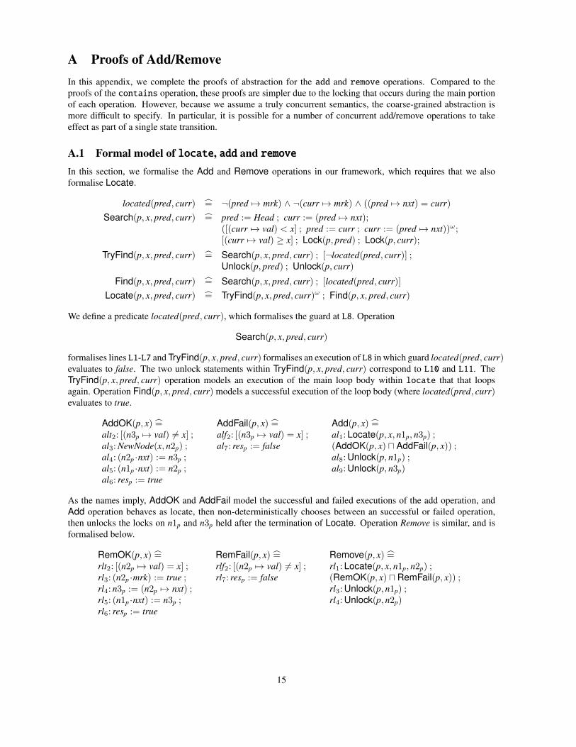
A Proofs of Add/RemoveIn this appendix, we complete the proofs of abstraction for the add and remove operations. Compared to theproofs of the contains operation, these proofs are simpler due to the locking that occurs during the main portionof each operation. However, because we assume a truly concurrent semantics, the coarse-grained abstraction ismore difficult to specify. In particular, it is possible for a number of concurrent add/remove operations to takeeffect as part of a single state transition.

A.1 Formal model of locate, add and removeIn this section, we formalise the Add and Remove operations in our framework, which requires that we alsoformalise Locate.

located(pred, curr) “= ¬(pred 7→ mrk) ∧ ¬(curr 7→ mrk) ∧ ((pred 7→ nxt) = curr)

Search(p, x, pred, curr) “= pred := Head ; curr := (pred 7→ nxt);([(curr 7→ val) < x] ; pred := curr ; curr := (pred 7→ nxt))ω;[(curr 7→ val) ≥ x] ; Lock(p, pred) ; Lock(p, curr);

TryFind(p, x, pred, curr) “= Search(p, x, pred, curr) ; [¬located(pred, curr)] ;Unlock(p, pred) ; Unlock(p, curr)

Find(p, x, pred, curr) “= Search(p, x, pred, curr) ; [located(pred, curr)]

Locate(p, x, pred, curr) “= TryFind(p, x, pred, curr)ω ; Find(p, x, pred, curr)

We define a predicate located(pred, curr), which formalises the guard at L8. Operation

Search(p, x, pred, curr)

formalises lines L1-L7 and TryFind(p, x, pred, curr) formalises an execution of L8 in which guard located(pred, curr)evaluates to false. The two unlock statements within TryFind(p, x, pred, curr) correspond to L10 and L11. TheTryFind(p, x, pred, curr) operation models an execution of the main loop body within locate that that loopsagain. Operation Find(p, x, pred, curr) models a successful execution of the loop body (where located(pred, curr)evaluates to true.

AddOK(p, x) “=alt2: [(n3p 7→ val) 6= x] ;al3: NewNode(x, n2p) ;al4: (n2p ·nxt) := n3p ;al5: (n1p ·nxt) := n2p ;al6: resp := true

AddFail(p, x) “=alf2: [(n3p 7→ val) = x] ;al7: resp := false

Add(p, x) “=al1: Locate(p, x, n1p, n3p) ;(AddOK(p, x) u AddFail(p, x)) ;al8: Unlock(p, n1p) ;al9: Unlock(p, n3p)

As the names imply, AddOK and AddFail model the successful and failed executions of the add operation, andAdd operation behaves as locate, then non-deterministically chooses between an successful or failed operation,then unlocks the locks on n1p and n3p held after the termination of Locate. Operation Remove is similar, and isformalised below.

RemOK(p, x) “=rlt2: [(n2p 7→ val) = x] ;rl3: (n2p ·mrk) := true ;rl4: n3p := (n2p 7→ nxt) ;rl5: (n1p ·nxt) := n3p ;rl6: resp := true

RemFail(p, x) “=rlf2: [(n2p 7→ val) 6= x] ;rl7: resp := false

Remove(p, x) “=rl1: Locate(p, x, n1p, n2p) ;(RemOK(p, x) u RemFail(p, x)) ;rl3: Unlock(p, n1p) ;rl4: Unlock(p, n2p)

15

A.2 The add operationIn this section, we verify the coarse-grained abstraction of the add operation. Unlike the contains operation,this abstraction cannot be defined using the standard language constructs, because the standard constructs are notprecise enough to describe the abstract behaviour. Hence, we introduce a specification command, which turns aninterval predicate to into a command, whose behaviour is given by the interval predicate. Thus, for an intervalpredicate g, process p and set of variables Z, the behaviour of a specification command is given by:

behp,Z . bgc “= g

We also introduce two further interval predicates, namely g, which states that interval predicate g holds andthe interval under consideration is non-empty, and 3g which states that g holds in some subinterval of the giveninterval, i.e., for an interval ∆ and stream s, we define:

g “= ¬empty ∧ g

(3g).∆.s “= ∃∆′: Interval • ∆′ ⊆ ∆ ∧ g.∆′.s

We define a state predicate WriteFields(p, a,F) which holds if process p writes to any of the fields in F of the datastructure at address a.

WriteFields(p, a,F) “= ∃b: a·f | f ∈ F •W.b.p

We further define interval predicate ModSet.p that is used to determine whether p ever writes to the addressescorresponding to the val, mrk and nxt fields of the nodes reachable from Head, IntFree(p, n), which holds if noother process different from p writes to fields of the node n, and Insert(p, x) that restricts the values that aremodified by p with respect to node n.

ModSet.p “= ∃a: setAddr • WriteFields(p, a, val,mrk, nxt)IntFree(p, n) “= ¬I.n·val, n·mrk, n·nxt, n·lck.p

Thus, ModSet.p holds iff there is a point in the interval such that p writes to the val, mrk or nxt fields of the node ataddress a and IntFree(p, n) holds iff there is no interference by the environment of p to any of the fields of node n.

The insertion of a node into the set is modelled as follows, where preIns denotes the precondition of an in-sertion, doIns models the insertion, and Insert models the full operation, including the possible interference fromother processors.

preIns(a, b, x) “= RE.Head.a ∧ located(a, b) ∧ (a 7→ val < x) ∧ (b 7→ val > x)

doIns(a, n, b, x) “= (a 7→ nxt = n) ∧ (n 7−→ (x, b, false, null))

Insert(p, x) “= ∃a, n, b: Addr • −−−−−−−−−→preIns(a, b, x) ∧ doIns(a, n, b, x) ∧

IntFree.a ∧ IntFree.b ∧ ∀ua: Addr\a·nxt • ¬W.ua.p

State predicate preIns(a, b, x) states that a is reachable from Head, the located(a, b) predicate holds, node ahas value is less than x and node b has value greater than x. Thus, x is not in the abstract set. State predicatedoIns(a, n, b, x) states that a · nxt is updated with value n, and node n has value x, points to b is not marked and isnot locked. The Insert(p, x) predicate states that there are addresses a, n and b such that preIns(a, b, x) holds as aprecondition, behaves as doIns(a, n, b, x) and furthermore, a and b are interference free and p does not write to anyother set address.

The coarse-grained abstraction of the add operation is then defined as follows.

CGAOK(p, x) “= ⌊Insert(p, x)

⌋; resp := true

CGAFail(p, x) “= 〈x ∈ absSet〉 ; resp := false

CGAdd(p, x) “= b¬ModSet.pc ; (CGAOK(p, x) u CGAFail(p, x)) ; b¬ModSet.pc

16

A successful execution of the add operation behaves as Insert(p, x) then sets the return value resp to true. A failedexecution of the add operation never adds n2p to the set, but detects that x is in the set and sets resp to false. TheAdd operation performs some idling at the start modelled as ¬ModSet.p because the concrete operation has thepossibility of not terminating, and at the end (to allow the concrete program time to unlock the held locks).

Like the decomposition depicted in Fig. 7 for the contains operation, we may decompose the proof so thatwe consider the execution of add by a single process under a rely condition r that we assume splits, provided thatthe rest of the program satisfies the rely condition that we derive. Given that CGS′ is the program derived fromCGS by replacing Add by CGAdd, the refinement holds if we prove both of the following:

RELY r • CGS′(p) vHTp S(p) (12)

behQ,HT .(‖q:Q S(q)) V r (13)

A.2.1 Proof of (12).

We define the following state predicate, which formalises the postcondition of Locate(p, pred, curr).

postLocate(p, pred, curr) “= located(pred, curr) ∧((pred 7→ val) < x) ∧ ((curr 7→ val) ≥ x) ∧((curr 7→ lck) = p) ∧ ((pred 7→ lck) = p) ∧RE.Head.pred ∧ RE.Head.curr

Thus, operation Locate ensures that pred and curr satisfy located, that the value of pred is less than x, the valueof curr is above or equal to x, that both curr and pred are locked, and that both pred and curr are reachable fromHead. We now have the following refinement, where U(p, n1, n2) “= Unlock(p, n1) ; Unlock(p, n2).

ENF r • Add(p, x)

vwMp definition of Add(p, x)

ENF r • Locate(p, x, n1p, n3p) ; (AddOK(p, x) u AddFail(p, x)) ; U(p, n1p, n3p)vwM

p logicENF r •

(ENF inf • Locate(p, x, n1p, n3p)) u (ENF fin • Locate(p, x, n1p, n3p))

);

(AddOK(p, x) u AddFail(p, x)) ; U(p, n1p, n3p)

wMp behaviour of Locate(p, x, n1p, n3p)

distribute ‘u’ over ‘;’, inf is a right annihilatorENF r • binf ∧ ¬ModSet.pc uENF r • (ENF fin • Locate(p, x, n1p, n3p)) ;

(AddOK(p, x) u AddFail(p, x)) ; U(p, n1p, n3p)

vwMp distribute ‘u’

ENF r • binf ∧ ¬ModSet.pc u (A1)ENF r • (ENF fin • Locate(p, x, n1p, n3p)) ; AddOK(p, x) ; U(p, n1p, n3p) u (A2)ENF r • (ENF fin • Locate(p, x, n1p, n3p)) ; AddFail(p, x) ; U(p, n1p, n3p) (A3)

Splitting the behaviour of Locate(p, x, n1p, n3p) into finite and infinite executions, and distributing the ‘;’through ‘u’, it is possible to show that CGAdd(p, x) vwL

p (CA1)u (CA2)u (CA3) where (CA1), (CA2), and (CA3)are defined below.

binf ∧ ¬ModSet.pc (CA1)bfin ∧ ¬ModSet.pc ; CGAOK(p, x) ; b¬ModSet.pc (CA2)bfin ∧ ¬ModSet.pc ; CGAFail(p, x) ; b¬ModSet.pc (CA3)

Proof of (A1). It is trivial to verify (CA1) vL,Mp (A1).

17

Proof of (A2). To prove this case, we strengthen condition r and require that it satisfies both of the following.

r V ((pcp ∈ ali | i ∈ [2, 7])⇒ IntFree.n1p ∧ IntFree.n3p) (14)r V (pcp ∈ al4, al5)⇒ stable.n2p ·val, n2p ·mrk, n2p ·nxt (15)

Assuming that r holds, we now have the following calculation.

behp,M.(ENF fin • Locate(p, x, n1p, n3p) ; AddOK(p, x) ; U(p, n1p, n3p)

)V expand behaviour and use (14)

behp,M.(ENF fin • Locate(p, x, n1p, n3p)) ;(IntFree.n1p ∧ IntFree.n3p ∧ behp,M.AddOK(p, x)) ;behp,M.U(p, n1p, n3p)

V first chop: behaviour of Locatesecond chop: expand AddOk(p, x), use postLocate, behaviour of alt2 and IntFree conditions

(¬ModSet.p ∧ −−−−−−−−−−−−−−−−→postLocate(p, n1p, n3p)) ;Ü∃a: Addr, k: Val •

Ñ(n1p 7→ val < x) ∧ (n3p 7→ val > x) ∧Å

behp,M.(alt2 ; al3 ; al4);(pcp = al5) ∧ evalp,M.(n1p ·nxt = a ∧ n2p = k)

ãé;

((pcp = al5) ∧ updatep,M.(a, k))

ê;

behp,M.al6 ; behp,M.U(p, n1p, n3p)V first chop: logic, second chop: expand behaviour use (15)¬ModSet.p ;Ö∃a: Addr, k: Val •

ǬModSet.p ∧ −−−−−−−−−−−−→preIns(n1p, n3p, x) ∧ (

−−−−−−−−−−−−−−−−−→n2p 7→ (x, n3p, false, null)) ∧

−−−−−−−−−−−−−−−−−→(n1p ·nxt = a ∧ n2p = k)

å;

((pcp = al5) ∧ updatep,M.(a, k))

è;

behp,M.al6 ; behp,M.U(p, n1p, n3p)≡ logic, ¬ModSet.p both splits and joins¬ModSet.p ;Ö∃a: Addr, k: Val •

Ç−−−−−−−−−−−−→preIns(n1p, n3p, x) ∧ (

−−−−−−−−−−−−−−−−−→n2p 7→ (x, n3p, false, null)) ∧

−−−−−−−−−−−−−−−−−→(n1p ·nxt = a ∧ n2p = k)

å∧

((pcp = al5) ∧ updatep,M.(a, k))

è;

behp,M.al6 ; behp,M.U(p, n1p, n3p)V p holds locks on n1p and n3p, use (15), definition of update¬ModSet.p ;Ç−−−−−−−−−−−−→preIns(n1p, n3p, x) ∧ doIns(n1p, n2p, n3p, x) ∧

IntFree.n1p ∧ IntFree.n3p ∧ ∀ua: Addr\a·nxt • ¬W.ua.p

å;

behp,M.al6 ; behp,M.U(p, n1p, n3p)V change context

behp,L.(CA2)

Proof of (A3). Once again assuming r holds, we obtain:

behp,M.(ENF fin • Locate(p, x, n1p, n3p) ; AddFail(p, x) ; U(p, n1p, n3p)

)V definition of beh and behaviour of Locate

(¬ModSet.p ∧ −−−−−−−−−−−−−−−−→postLocate(p, n1p, n3p)) ; behp,M.AddFail(p, x) ; behp,M.U(p, n1p, n3p)V definition of postLocate(p, n1p, n3p)Ç

behp,L.Idle ∧−−−−−−−−−−−−−−−−−−−−−−→RE.Head.n3p ∧ ¬(n3p 7→ mrk)

å; behp,M.AddFail(p, x) ; behp,M.U(p, n1p, n3p)

V use (14) and guard alf3, change contextbehp,L.Idle ; (behp,L.Idle ∧ (RE.Head.n3p ∧ ¬(n3p 7→ mrk) ∧ (n3p 7→ val = x))) ;

behp,M.(al7 ; U(p, n1p, n3p))

18

V definition of absSetbehp,L.Idle ; (behp,L.Idle ∧ (x ∈ absSet)) ; behp,M.(al7 ; U(p, n1p, n3p))

V change contextbehp,M.CA3

A.2.2 Proof of (13).

We strengthen the rely condition with additional conjunct (14) ∧ (15). This proof is straightforward due to thelocks held by process p.

A.3 The remove operationA coarse-grained abstraction of the remove operation is given below.

preDel(p, a, n, b, x) “= RE.Head.a ∧ located(a, n) ∧ (a 7→ val < x) ∧(n 7−→ (x, b, false, p))

doDel(a, n, b, x) “= ((a 7→ nxt = b) ∨ (n 7→ mrk))

Delete(p, x) “= ∃a, n, b: Addr • −−−−−−−−−−−−−→preDel(p, a, n, b, x) ∧ doDel(a, n, b, x) ∧

IntFree.a ∧ IntFree.n ∧∀ua: Addr\a·nxt, n·mrk • ¬W.ua.p

CGROK(p, x) “= ⌊Delete(p, x)

⌋; resp := true

CGRFail(p, x) “= 〈x 6∈ absSet〉 ; resp := false

CGR(p, x) “= b¬ModSet.pc ; (CGROK(p, x) u CGRFail(p, x)) ; b¬ModSet.pc

The proof of refinement between remove and the abstraction above proceeds in a similar manner to the addoperation. In particular, CGR(p, x) vL

p (CR1) u (CR2) u (CR3) holds, where:

binf ∧ ¬ModSet.pc (CR1)bfin ∧ ¬ModSet.pc ; CGROK(p, x) ; b¬ModSet.pc (CR2)bfin ∧ ¬ModSet.pc ; CGRFail(p, x) ; b¬ModSet.pc (CR3)

Furthermore, (R1) u (R2) u (R3) vL,Mp Remove(p, x) holds, where:

(ENF inf • Locate(p, x, n1p, n2p)) (R1)(ENF fin • Locate(p, x, n1p, n2p)) ; RemOK(p, x) ; U(p, n1p, n2p) (R2)(ENF fin • Locate(p, x, n1p, n2p)) ; RemFail(p, x) ; U(p, n1p, n2p) (R3)

Thus, to complete the proof, we must show: (CRi) vL,Mp (Ri) for i ∈ 1, 2, 3, and the proof of i = 3 is similar to

the failed case of the add. The proof of i = 1 is trivial. For the proof of case i = 2 we assume the following.

r V ((pcp ∈ rli | i ∈ [2, 7])⇒ IntFree.n1p ∧ IntFree.n2p) (16)

Hence, assuming r, the proof proceeds as follows.

behp,M.(R2)≡ expanding definitions

behp,M.(ENF fin • Locate(p, x, n1p, n2p)) ;Å∃a: Addr, k: Val • behp,M.rlt2 ; ((pcp = rl3) ∧ evalp,M.(k ∧ (a = (n2p ·mrk)))) ;

((pcp = rl3) ∧ updatep,M.(a, k)) ; behp,M.(rl4 ; rl5 ; rl6)

ã;

behp,M.U(p, n1p, n2p)V behaviour of Locate, then assuming (16)

(¬ModSet.p ∧ −−−−−−−−−−−−−−−−→postLocate(p, n1p, n2p)) ;

19

Å∃a: Addr, k: Val • behp,M.rlt2 ; ((pcp = rl3) ∧ evalp,M.(k ∧ a = (n2p ·mrk))) ;

((pcp = rl3) ∧ updatep,M.(a, k)) ; behp,M.(rl4 ; rl5 ; rl6)

ã;

behp,M.U(p, n1p, n2p)V logic, expand behaviours, use (16)¬ModSet.p ;Ç∃b: Addr • ¬ModSet.p ∧ −−−−−−−−−−−−−−−−→postLocate(p, n1p, n2p) ∧ −−−−−−−−−−−−−−−−→(n2p 7−→ (x, b, false, p)) ;

((pcp = rl3) ∧ updatep,M.(n2p ·mrk, true)) ; behp,M.(rl4 ; rl5 ; rl6)

å;

behp,M.U(p, n1p, n2p)≡ ¬ModSet.p splits and joins, logic¬ModSet.p ;Ç∃b: Addr • (

−−−−−−−−−−−−−−−−→postLocate(p, n1p, n2p) ∧ −−−−−−−−−−−−−−−−→(n2p 7−→ (x, b, false, p))) ∧

((pcp = rl3) ∧ updatep,M.(n2p ·mrk, true)) ; behp,M.(rl4 ; rl5 ; rl6)

å;

behp,M.U(p, n1p, n2p)V behaviour definitions, (16)

behp,M.(CR2)

Finally, we are left with a proof requirement that the rest of the program implies the rely condition (16). This proofis straightforward due to the locks held by process p.

20