simualation of electro-hydraulic servo actuator
TRANSCRIPT

SIMUALATION OF ELECTRO-HYDRAULIC SERVO ACTUATOR
A Thesis submitted in partial fulfillment of the requirements for
the degree of
Master of Technology in Mechanical Engineering (Machine Design and Analysis Specialization)
By
Vijaya Sagar Tenali
Department of Mechanical Engineering National Institute of Technology, Rourkela
Rourkela-769008(Orissa)
1

SIMULATION OF ELECTRO-HYDRAULIC SERVO ACTUATOR
A Thesis submitted in partial fulfillment of the requirements for
the degree of
Master of Technology in Mechanical Engineering (Machine Design and Analysis Specialization)
By
Vijaya Sagar Tenali
Under the esteemed guidance of
Sri S.Viswanath (Co-guide) Deputy General Manager RWRDC HAL, Bangalore
Sri S.C.Mohanty (Guide) Senior Lecturer, Mechanical Engg Dept. NIT Rourkela.
Department of Mechanical Engineering National Institute of Technology, Rourkela
Rourkela-769008(Orissa)
2

BONAFIDE CERTIFICATE
This is to certify that the thesis entitled “SIMULATION OF ELECTRO-HYDRAULIC
SERVO ACTUATOR”, submitted by Mr. Vijaya Sagar Tenali for the award of the
degree of Master of Technology (Machine design & Analysis) of National Institute of
Technology is product of research work carried out by him under my/our guidance.
Mr.Vijaya Sagar Tenali has worked on the above problem at Hydraulics group, RWRDC,
HAL Bangalore and this has reached the standard of fulfilling the requirements and the
regulation to the degree. The contents of this thesis, in full or in part, have not been
submitted to any other university or institution for the award of any degree or diploma.
Co Guide
Sri S.Viswanath
Deputy General Manager
RWRDC
HAL, Bangalore.
Guide Sri S.C.Mohanty
Sr Lecturer
Mechanical Engg Dept
NIT Rourkela
3
ACKNOWLEDGEMENT
I extend my deep sense of indebtedness and gratitude to my guide Dr.S.C. Mohanty,
Senior Lecturer, Department of Mechanical Engineering, National Institute of
Technology, Rourkela , for providing me an opportunity to work under his supervision
and guidance .His keen interest, invaluable guidance, immense help have helped me to
successfully complete my thesis.
I am also extremely grateful to Mr.S.Viswanath, Deputy General Manager, Rotary Wing
Research & Design Centre, HAL Bangalore for his unfailing inspiration, whole hearted
cooperation and fruitful discussions which are embodied in this thesis. His sincere
sympathies and kind attitude always encouraged me to carry out my present work firmly.
I am also thankful to Dr B.K.Nanda Professor and Head of the Department Of
Mechanical Engineering, National Institute of Technology Rourkela for providing all
kinds of help throughout for the completion of the thesis.
It is a great pleasure for me to acknowledge and express my gratitude to my friends
K.Damodaran, Krishna Kishore and Ganesh for their help and support during my study.
Lastly, I thank all those who are involved directly or indirectly in completion of the
present thesis work.
Vijaya Sagar Tenali
4

CONTENTS Page No
1. Introduction to Helicopter motion control 1-6
1.1 Comparative Study Between Fixed Wing (Aero Plane) & Rotary Wing 4
(Helicopter)
1.2 Role Of Hydraulics In Helicopter Flight Control 5
2. Introduction 7-21
2.1 Hydraulic System Description 7
2.1.1 Hydraulic Power Supply 9
2.1.2 Hydraulic Supply Pressure Selection 11
2.1.3 Flow Control Valve 11
2.1.4 Linear Hydraulic Actuator 15
2.2. Selection of Hydraulic Actuator 15
2.3 Description of the Actuator 16
2.4. Definitions 18
2.4.1 Valve Nomenclature 18
2.4.2 Electrical Input Characteristics 19
2.4.3 Static Performance Characteristics 19
2.5. About Simulink 20-21
3. Literature Survey 22-26
3.1 Introduction 22
3.2 Simulation of Hydraulic Actuators 22
4. Mathematical modeling of the Hydraulic system 27-36
4.1. Mathematical modeling of flow control servo valve 27
4.1.1 Torque motor 27
5

4.1.2 Modeling Valve Flow Pressure 30-31
4.2 Modeling Linear Actuator 32-34
4.2.1 Cylinder chamber pressure 32
4.2.2 Piston Dynamics 33
4.3 Modeling of Hydraulic Power Supply 35
4.4 Modeling of Servo Controller 36
5. Numerical Simulation Data Used In The Present Study 37
6. Simulink Models 38-47
7. Results and Discussion 48-56
8. Conclusions 57
9. Scope for Future Development 58
10. References 59-62
6

ABSTRACT Hydraulic actuators are used in many applications like aircraft flight control,
machinery and automobiles etc. This actuator when coupled with a feedback system is
called a Servo Actuator. The response of the hydraulic actuator with time is significant
particularly when the actuator is used for flight control operations. So finding the time
response of the particular hydraulic actuator much before its actual operation will be very
helpful for the designer for analyzing the performance of the system. This also helps the
designer to arrive at optimum design parameters of the hydraulic actuator. In this thesis a
position control electro-hydraulic linear actuator is selected. This actuator is used for
controlling the movements of the helicopter. Mathematical modelling of the hydraulic
actuator and its components is done and based on the mathematical equations
Matlab/Simulink models of the actuator and its components were made and the time
response of the linear actuator is obtained by using Matlab/Simulink Software. The time
response graphs which are obtained in this simulation are found to be in good
compromise with the time response graphs of Moog experimental time response graphs.
7

LIST OF FIGURES
Figure Title of figure Page No.
No.
1.1 Fundamental Parts of Helicopter 1
1.2 Types of Flight control 2
1.3 Differential Control 3
1.4 Collective Control 4
1.5 Helicopter flight control system 6
2.1 Block diagram of apposition controlled Hydraulic servo system 10
2.2 diagram of three land, four way flow control valve 13
2.3 Cross section of nozzle flapper type servo valve 14
2.4 Cross section diagram of Double-ended, Double-acting Linear Actuator 17
4.1 Valve Torque motor Assembly 28
4.2 Valve responding to change in electrical input 29
6.1 Simulink model of top level hydraulic system. 39
6.2 Simulink model of hydraulic Actuator 40
6.3 Simulink Model of Servo valve 41
6.4 Simulink model of piston chamber ‘A’ of the actuator 42
6.5 Simulink model of piston chamber ‘B’ of the actuator 43
6.6 Simulink model of servo controller 44
6.7 Simulink model of servo controller subsystem 45
6.8 Simulink model of pressure supply subsystem 46
6.9 Simulink model of LVDT subsystem 47
8

Figure Title of figure Page No.
No.
7.1 Time response of linear hydraulic actuator 50
7.2 Time response of Piston Chamber ‘A’ of the Actuator 51
7.3 Time response of Piston Chamber ‘B’ of the Actuator 52
7.4 Time response of the Actuator 53
7.5 Time response of the servo valve 54
7.6 Experimental time response graph of Hydraulic Actuator 55
7.7 experimental Time response graph in Piston chambers ‘A’ and ‘B’ 56
9

LIST OF TABLE Page No. Table 1.1 comparative study between fixed wing (aeroplane) 4
& rotary wing (helicopter)
10

NOMENCLATURE
AP = Active area of the piston annulus Be = Bulk Modulus of the hydraulic fluid dVA = Rate of change of volume of chamber A dVB = Rate of change of volume of chamber B FP = Force generated across piston annulus LC = Inductance of the servo valve MP = Mass of the actuator piston PA = Oil Pressure at actuator port A PB = Oil Pressure at actuator port B PR = Pressure drop in return Line to tank PS = Supply pressure from hydraulic pump QA = Oil flow at servo valve at servo valve port A QB = Oil flow at servo valve at servo valve port B QL = Total flow through the load
QP = Maximum oil flow capacity of the pump Qr = Rated flow of servo valve at 70 bar pressure drop RC = Series resistance of the Torque motor circuit Ue = Error output from summing Amplifier Up = Feedback signal from displacement transducer
11

Uv = Command signal to servo valve VA = Volume of trapped oil in chamber A of the Cylinder VB = Volume of trapped oil in chamber B of the cylinder Vt = Volume of trapped between pump and servo valve
Xp = Displacement of the piston relative to centre position
12

1. INTRODUCTION TO HELICOPTER MOTION
CONTROL
A Helicopter is a Rotorcraft that derives its lift from one or more power driven rotors.
(A rotor is a system of rotating aerofoil.). Helicopters offer a facility to move from
one place to other, which are remotely located, and not having well laid out runway
which are otherwise required for fixed wing planes. Helicopters serve various
purposes from to civil transport, ambulance, police, and forest fire prevention to
sophisticated military application.
Figure 1.1 Generally one or two turbo shaft engines provide the power to the rotor system
through a speed reduction gearbox to run the rotor at a constant speed. A rotor at the tail
with a moment arm provides anti torque to the main body of the helicopter called the
Fuselage. Accessory driven gear box provides facility for Hydraulic pump, electrical
generator and other utility power outlets at various speeds. Modern helicopters utilize
digital display and communication for information transfer from one system to other and
there by extracting the optimum performance out of the flight vehicle.
Helicopters have two type of flight control mechanism to control the pitch angle
of four main Rotor blades.
1. Differential control (Pitch & Roll)
2. Collective pitch control
3. Yaw control
13

In Differential control opposite blades being tilted in opposite direction.i.e. clockwise &
anticlockwise. Hence Differential lift force creates the couple, which in turn tilts the
plane of rotation. This changes the direction of resultant force which results turn of
Helicopter itself. Pitch & Roll controls are achieved through this mode only.
In collective control, all the four blades are tilted n the same direction. i.e. pitch angle of
all the blades being changed uniformly. The result is Change in the lift force. There is no
change in the direction of force. Only magnitude gets changed.
Yaw control requires, tail rotor blade pitch control. By increasing the pitch angle, the
thrust force produced by the tail rotor blades is increased which in turn creates a moment
and hence helicopter turns in the lateral direction.
Three types of flight Control:
Figure 1.2
14

Differential Control Figure 1.3
Collective control
Collective Control
Figure 1.4
15
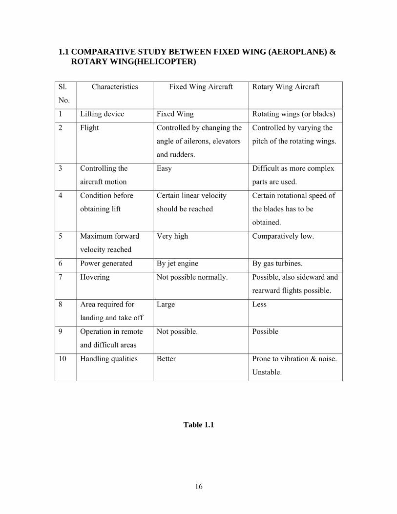
1.1 COMPARATIVE STUDY BETWEEN FIXED WING (AEROPLANE) & ROTARY WING(HELICOPTER)
Sl.
No.
Characteristics Fixed Wing Aircraft Rotary Wing Aircraft
1 Lifting device Fixed Wing Rotating wings (or blades)
2 Flight Controlled by changing the
angle of ailerons, elevators
and rudders.
Controlled by varying the
pitch of the rotating wings.
3 Controlling the
aircraft motion
Easy Difficult as more complex
parts are used.
4 Condition before
obtaining lift
Certain linear velocity
should be reached
Certain rotational speed of
the blades has to be
obtained.
5 Maximum forward
velocity reached
Very high Comparatively low.
6 Power generated By jet engine By gas turbines.
7 Hovering Not possible normally. Possible, also sideward and
rearward flights possible.
8 Area required for
landing and take off
Large Less
9 Operation in remote
and difficult areas
Not possible. Possible
10 Handling qualities Better Prone to vibration & noise.
Unstable.
Table 1.1
16

1.2 ROLE OF HYDRAULICS IN HELICOPTER FLIGHT CONTROL
Nowadays Helicopter flight control in the most common configurations is
realized by collective and cyclic variation of the angle of attack of each rotor blade. The
Collective blade control pitches the rotor blades to equal angles of attack around their
longitudinal axis, changing the rotor thrust at constant rotor speed. Yaw and roll control
is realized via cycle blade motion by changing the angle of attack of every rotor blade
locally and periodically during one revolution.
The control of the rotor blade angles for small helicopters is done manually by
the pilot with the help of push-pull rods .But for a bigger helicopter the aerodynamic
forces acting on the rotor blade are so high that it becomes impossible to control the rotor
blade angles manually for the pilot. So for medium and large helicopters the control of
the rotor blade angles is done with the help of hydraulic Actuators. These hydraulic
actuators help in controlling the roll, pitch and collective Movements of the helicopter.
17

Figure 1.5 Helicopter flight Control system
18
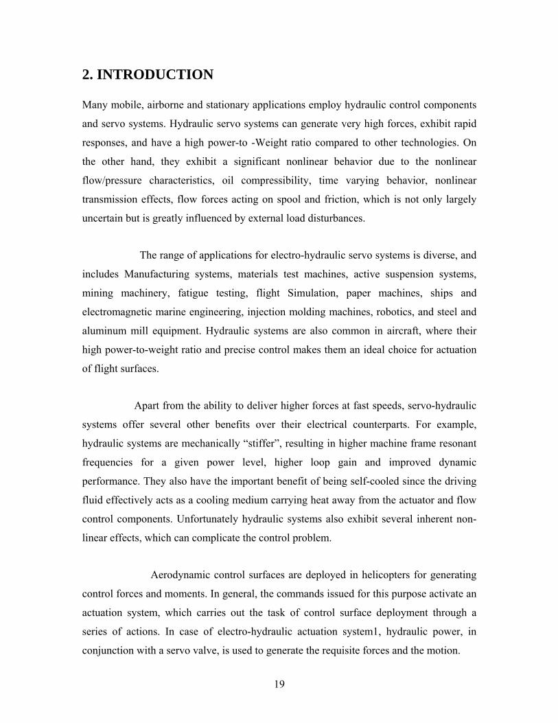
2. INTRODUCTION
Many mobile, airborne and stationary applications employ hydraulic control components
and servo systems. Hydraulic servo systems can generate very high forces, exhibit rapid
responses, and have a high power-to -Weight ratio compared to other technologies. On
the other hand, they exhibit a significant nonlinear behavior due to the nonlinear
flow/pressure characteristics, oil compressibility, time varying behavior, nonlinear
transmission effects, flow forces acting on spool and friction, which is not only largely
uncertain but is greatly influenced by external load disturbances.
The range of applications for electro-hydraulic servo systems is diverse, and
includes Manufacturing systems, materials test machines, active suspension systems,
mining machinery, fatigue testing, flight Simulation, paper machines, ships and
electromagnetic marine engineering, injection molding machines, robotics, and steel and
aluminum mill equipment. Hydraulic systems are also common in aircraft, where their
high power-to-weight ratio and precise control makes them an ideal choice for actuation
of flight surfaces.
Apart from the ability to deliver higher forces at fast speeds, servo-hydraulic
systems offer several other benefits over their electrical counterparts. For example,
hydraulic systems are mechanically “stiffer”, resulting in higher machine frame resonant
frequencies for a given power level, higher loop gain and improved dynamic
performance. They also have the important benefit of being self-cooled since the driving
fluid effectively acts as a cooling medium carrying heat away from the actuator and flow
control components. Unfortunately hydraulic systems also exhibit several inherent non-
linear effects, which can complicate the control problem.
Aerodynamic control surfaces are deployed in helicopters for generating
control forces and moments. In general, the commands issued for this purpose activate an
actuation system, which carries out the task of control surface deployment through a
series of actions. In case of electro-hydraulic actuation system1, hydraulic power, in
conjunction with a servo valve, is used to generate the requisite forces and the motion.
19

The desired motion is achieved through a closed loop feedback control system that senses
the actual deflection and corrects it until the desired position is reached. In recent times,
there has been a trend towards designing higher agility aerospace vehicles resulting in
larger bandwidths, as well as higher actuation rates, of actuation systems.
Electro hydraulic Servo System (EHSS) is a closed loop control system,
which is usually applied as an actuator unit to drive an object such as a rudder or vane.
Depending on variable to be controlled, it can be a position, velocity or force control
system. Electro hydraulic servo systems have the advantages of, precise and fine control,
high power to weight ratio, small size, good load matching, high environmental stiffness,
fast dynamic performances and wide adjustable speed range. Large inertia and torque
loads can be handled with high accuracy and very rapid response. All these advantages
are suitable for aerospace and missile applications.
20
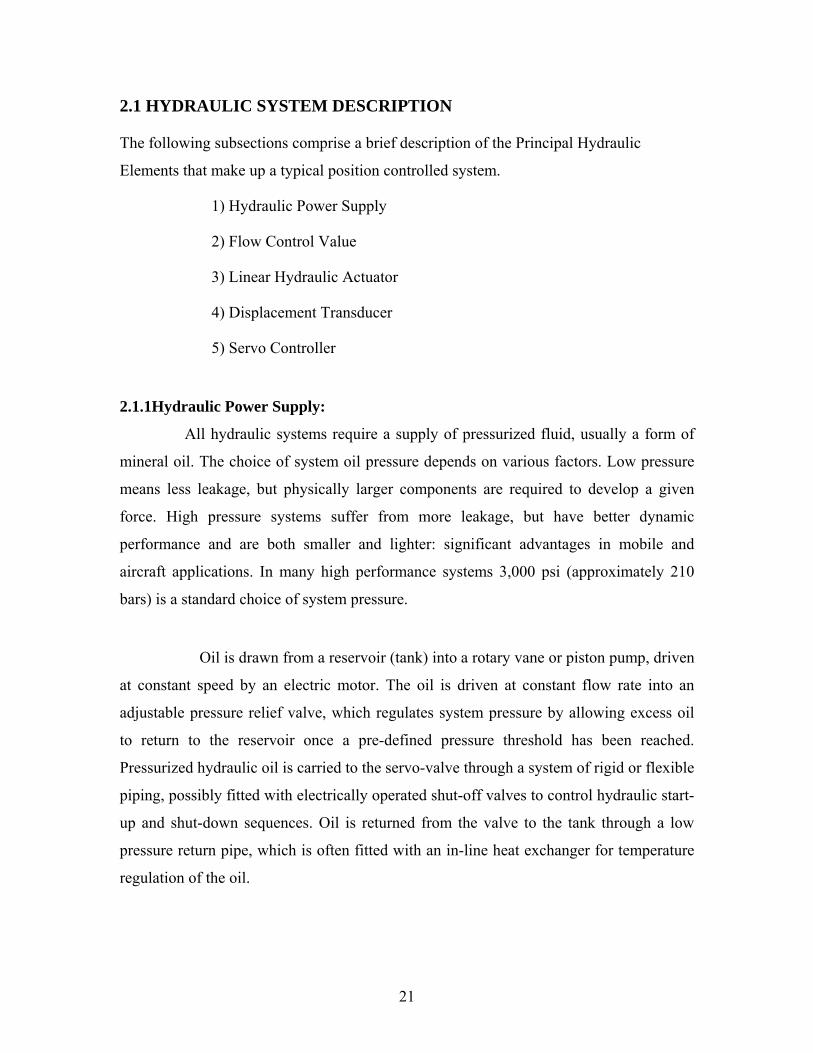
2.1 HYDRAULIC SYSTEM DESCRIPTION
The following subsections comprise a brief description of the Principal Hydraulic
Elements that make up a typical position controlled system.
1) Hydraulic Power Supply
2) Flow Control Value
3) Linear Hydraulic Actuator
4) Displacement Transducer
5) Servo Controller
2.1.1Hydraulic Power Supply:
All hydraulic systems require a supply of pressurized fluid, usually a form of
mineral oil. The choice of system oil pressure depends on various factors. Low pressure
means less leakage, but physically larger components are required to develop a given
force. High pressure systems suffer from more leakage, but have better dynamic
performance and are both smaller and lighter: significant advantages in mobile and
aircraft applications. In many high performance systems 3,000 psi (approximately 210
bars) is a standard choice of system pressure.
Oil is drawn from a reservoir (tank) into a rotary vane or piston pump, driven
at constant speed by an electric motor. The oil is driven at constant flow rate into an
adjustable pressure relief valve, which regulates system pressure by allowing excess oil
to return to the reservoir once a pre-defined pressure threshold has been reached.
Pressurized hydraulic oil is carried to the servo-valve through a system of rigid or flexible
piping, possibly fitted with electrically operated shut-off valves to control hydraulic start-
up and shut-down sequences. Oil is returned from the valve to the tank through a low
pressure return pipe, which is often fitted with an in-line heat exchanger for temperature
regulation of the oil.
21

Figure 2.1 Block diagram of a position controlled Hydraulic Servo system
22

2.1.2 Hydraulic Supply Pressure Selection:
One of the first steps in design of a hydraulic control system is to select
supply pressure. Many considerations favor a large supply pressure. Power is the product
of pressure and flow. As supply pressure is increased, less flow is required to provide a
given power. Smaller Pump, lines, valves, oil supply etc are then possible. Faster
response is often possible because of small oil volume and higher bulk modulus. Thus
high pressure in EHSS improves power to weight ratio and reduce size of the components
and overall weight. The development of aerospace, aviation and missiles technology
require, light weight, small volume, high pressure, high power and multi redundant and
intelligent control.
2.1.3 Flow Control Valve:
The electro-hydraulic flow control valve acts as a high gain electrical to
hydraulic transducer, the input to which is an electrical voltage or current, and the output
a variable flow of oil. The valve consists of a spool with lands machined into it, moving
within a cylindrical sleeve. The lands are aligned with apertures cut in the sleeve such
that movement of the spool progressively changes the exposed aperture size and alters
differential oil flow between two control ports.
The vast majority of flow control servo valves in existence employ a
double flapper nozzle pilot stage and a single spool boost stage. A stiff feedback spring is
generally used to provide feedback from the boost stage to the pilot. These types of servo
valves tend to be difficult to manufacture and expensive. A less conventional, less costly
type of flow control servo valve utilizes a two-spool boost stage and a flapper nozzle
pressure control pilot. Because a feedback wire between the nozzle flapper pilot and the
boost stage is not needed, assembly is simplified. The two spools in the boost stage are
spring-loaded and meter flow into and out of the valve separately. The main advantages
23

of the two-spool/ pressure control pilot designs are 1) ease of manufacturing 2) lower
costs 3) higher degree of adjustment; and 4) Greater safety.
Figure 2.2 shows the spool configuration of a typical “3-4” flow
control valve. The ports are labeled P (pressure), T (tank), and A and B (load control
ports). The spool is shown displaced a small distance (xv) as a result of a command force
applied to one end, and arrows at each port indicate the direction of fluid flow, which
results. With no command force applied (Fv=0), the spool is centralized and all Ports are
closed off by the lands resulting in no load flow.
In the context of hydraulic servo-systems, flow control valves fall broadly into two main
categories:
Proportional valves and servo-valves. Proportional valves use direct actuation of
the spool from an electrical solenoid or torque motor, whereas servo-valves use at least
one intermediate hydraulic amplifier stage between the electrical torque motor and the
spool.
The basic servo-valve produces a control flow proportional to input current for a
constant load. While the dynamic performance of a servo-valve is influenced somewhat
by operating conditions (supply pressure, input signal level, fluid and ambient
temperature and so on) a major advantage is that load dynamics do not affect stability,
unlike single stage proportional valves. Servo valves usually have superior dynamic
response, although their close internal machining tolerances make them relatively
expensive and susceptible to contamination of the hydraulic fluid.
Two stage servo-valves may be further divided into nozzle-flapper and jet pipe types.
Both use a similar design of electromagnetic torque motor, but the hydraulic amplifier
circuits are radically different. Nozzle-flapper type servo-valves are currently by far the
most common in high performance servo applications and the description, which follows,
is based on this type of valve.
24

A cross sectional view of a typical nozzle-flapper type servo-valve is shown in figure 2.3.
High pressure hydraulic oil is supplied at the inlet pressure port (P), and a low pressure
return line to the oil reservoir is connected to the tank port (T). The two hydraulic control
ports (A and B) carry the control oil flows to and from the load actuator.
Figure 2.2 Diagram of Three Land, Four Way Flow Control Valve
25

Figure 2.3 showing Cross Section of Nozzle Flapper Type Servo valve
26
2.1.4 Linear Hydraulic Actuator:
Linear actuators are the devices for converting fluid power into linear motion.
They may be used to exert a force, to hold or clamp, and to initiate or stop motion. All
linear actuators are some modification of an air or hydraulic cylinder and may be either
single or double acting .the single acting cylinder receives power at one end only and is
returned to its original position by gravity or by spring action, while double acting
cylinder is powered in both directions. Double-acting cylinders permit more complete
control of movement. Ram is a form of single acting cylinder in which the piston rods are
of the same diameter.
The double rod cylinder has a rod attached to both sides of the piston. This type
of cylinder is center-mounted and is normally used when the same task is performed at
the either end on staggered cycles. Obviously the force and speed will be the same at
either end.
2.2. Selection of Hydraulic Actuator
Actuator is the key component of hydraulic servo system.
1) Its size should be large enough not only to handle the loads expected during duty
cycle but also ensure the required load velocity. It is also important not to
oversize actuators so that the flow required for maximum velocity is kept to a
minimum. Otherwise, the hydraulic power supply becomes bulky with large no
load power losses.
2) The load should be properly matched to the output of the system. Load matching
effectively utilizes the output power of hydraulic source and improves
performance of
the hydraulic system.
27

3) Other important Actuator performance characteristics, which might be important,
are speed, range, stiffness of the smoothness (i.e., absence of velocity variations at
operating speeds).
4) Reliability
5) Backlash
6) Pressure rating
7) Cost
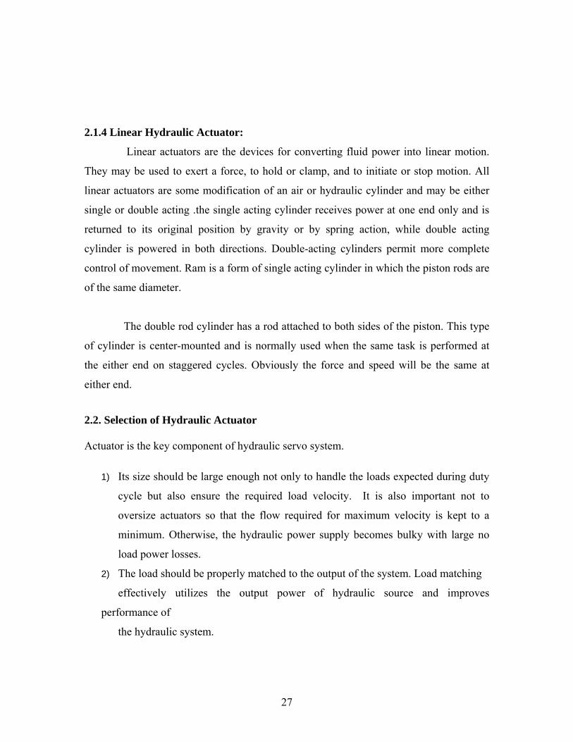
2.3 DESCRIPTION OF THE ACTUATOR:
The description which follows is based on a linear, double-acting, double-ended actuator:
a type used in many industrial applications. A cross section of such an actuator is shown
in figure 2.4. The actuator consists of a rod and central annulus, and incorporates low
friction seals fitted to the piston annulus and at each of the cylinder end caps to minimize
leakage. Control ports are drilled into each end of the cylinder to allow hydraulic fluid to
flow in and out of the two chambers.
The position of the piston is determined by the hydraulic fluid pressures in the chambers
on either side of the central annulus, and may be adjusted by forcing fluid into one
control port while allowing it to escape from the other. In the diagram above, hydraulic
fluid is shown entering control port A while escaping from port B. This causes an
increase in fluid pressure in the chamber to the left of the piston annulus, and a decrease
in pressure in the right chamber. The net pressure difference exerts a force on the active
area of the annulus, which moves the piston to the right as shown. Adjustment of piston
position is therefore a matter of controlling the differential oil flow between the two-
actuator control ports.
28
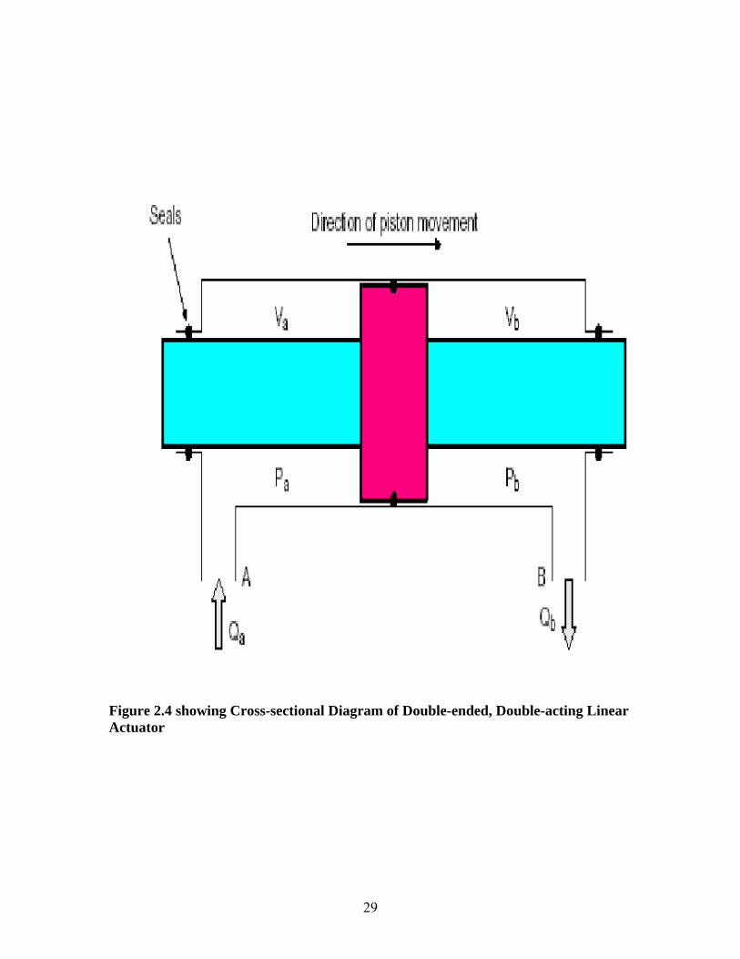
Figure 2.4 showing Cross-sectional Diagram of Double-ended, Double-acting Linear Actuator
29

2.4 DEFINITIONS
Servomechanism - A continuously acting, bidirectional closed-loop control system.
Servo valve - A device used to produce hydraulic control in a servomechanism.
Electro hydraulic Servo valve - A servo valve which produces hydraulic control in
response to electrical signal inputs; sometimes called a transfer valve.
Electro hydraulic Flow Control Servo valve - A servo valve designed to produce
hydraulic flow output proportional to electrical current input.
2.4.1 VALVE NOMENCLATURE
1. Hydraulic Amplifier -A fluid valving device which acts as a power amplifier, such as a
sliding spool, or a nozzle flapper, or a jet pipe with receivers.
2. Stage - The portion of a servo valve which includes a hydraulic amplifier. Servo valves
may be single stage, two stage, three stage, etc.
3. Output Stage -The final stage of hydraulic amplification used in a servo valve, usually
a sliding spool.
4. Port -A fluid connection to the servo valve; for example, a supply port, a return port, or
control port
5. Three-Way Valve - A multi-orifice fluid control element with supply, return and one
control port arranged so that valve action in one direction opens the control port to supply
and reversed valve action opens the control port to return.
6. Four-Way Valve - A multi-orifice fluid control element with supply, return and two
control ports arranged so that valve action in one direction simultaneously opens control
port #1 to supply and control port #2 to return. Reversed valve action opens control port
#1 to return and control port #2 to supply.
30

2.4.2 ELECTRICAL INPUT CHARACTERISTICS
1. Torque Motor - The electromechanical transducer commonly used with the input stage
of a servo valve. Displacement of the armature of the torque motor is generally limited
to a few thousandths of an inch.
2. Input Current -The current which is required for control of the valve, expressed in ma.
For three and four lead coils, input current is generally the differential coil current,
expressed in ma.
3. Rated Current - The specified input current of either polarity to produce rated flow,
4. Current must be associated with a specific coil connection.
2.4.3 STATIC PERFORMANCE CHARACTERISTICS
1. Control Flow, also called Load Flow or Flow Output the fluid flow passing through
the valve control ports, expressed in cis or gpm. In testing a four-way servo valve,
flow passing out one control port is assumed equal to the flow passing in the other.
This assumption is valid for no-load valve testing with a symmetrical load
2. Rated Flow - The specified control flow corresponding to rated current and specified
load pressure drop, expressed in cis or gpm. Rated flow is normally specified as the
no-load flow.
3. No-Load Flow - The servo valve control flow with zero load pressure drop, expressed
in cis or gpm.
4. Power Output -The fluid power which is delivered to the load, expressed in hp.
5. Flow Saturation - The condition where flow gain decreases with increasing input
current. Flow saturation may be deliberately introduced by mechanical limiting of the
valve range, or may be the result of increasing pressure drops along internal fluid
passages.
6. Flow Limit - The condition wherein control flow no longer increases with increasing
input current.
31

2.5. ABOUT SIMULINK
Simulink is a software package for modeling, simulating, and analyzing
dynamical systems. It supports linear and nonlinear systems, modeled in continuous time,
sampled time, or a hybrid of the two. Systems can also be multi rate, i.e., have different
parts that are sampled or updated at different rates.
For modeling, Simulink provides a graphical user interface (GUI) for building
models as block diagrams, using click-and-drag mouse operations. With this interface, we
can draw the models just as we would with pencil and paper. This is a far cry from
previous simulation packages that require us to formulate differential equations and
difference equations in a language or program. Simulink includes a comprehensive block
library of sinks, sources, linear and nonlinear components, and connectors. We can also
customize and create our own blocks.
Models are hierarchical, so we can build models using both top-down and
bottom-up approaches. We can view the system at a high level, and then double-click on
blocks to go down through the levels to see increasing levels of model detail. This
approach provides insight into how a model is organized and how its parts interact.
After we define a model, we can simulate it, using a choice of integration
methods, either from the Simulink menus or by entering commands in MATLAB’s
command window. The menus are particularly convenient for interactive work, while the
command-line approach is very useful for running a batch of simulations. Using scopes
and other display blocks, we can see the simulation results while the simulation is
running. In addition, we can change parameters and immediately see what happens, for
“what if” exploration. The simulation results can be put in the MATLAB workspace for
post processing and visualization.
32

Model analysis tools include linearization and trimming tools, which can be
accessed from the MATLAB command line, plus the many tools in MATLAB and its
application tool boxes. And because MATLAB and Simulink are integrated, we can
simulate, analyze, and revise our models in either environment at any point.
We can build models from scratch, or take an existing model and add to it.
Simulations are interactive, so we can change parameters and immediately see what
happens. We can have instant access to all of the analysis tools in MATLAB, so we can
take the results and analyze and visualize them.
With Simulink, we can move beyond idealized linear models to explore more
realistic nonlinear models, factoring in friction, air resistance, gear slippage, hard stops,
and the other things that describe real-world phenomena. It turns our computer into a lab
for modeling and analyzing systems that simply wouldn’t be possible or practical
otherwise, whether the behavior of an automotive clutch system, the flutter of an airplane
wing, the dynamics of a predator-prey model.
33

3. LITERATURE SURVEY
3.1 INTRODUCTION
Until now a lot of work has been done on control, operation and testing of
hydraulic systems. With the evolution of computer simulation techniques, this process
has become much simpler. There are many reports describing field experience related to
analyzing hydraulic actuators using Simulink software. In this chapter works published in
a wide spectrum of journals have analyzed and the goals for the present study have been
given a firm foundation with the information derived from the survey. They are presented
in the subsequent sections.
3.2 SIMULATION OF HYDRAULIC ACTUATORS The mathematical model for the hydraulic System is made with the help of system
characteristics and its behavior. With the help of these mathematical models various
hydraulic systems have been analyzed by using softwares like MATLAB, SIMULINK,
and SIMULATIONX etc.
Pramod[1] studied the effect of non-linearities in the configuration design of Digital
Auto Pilot (DAP) in launch vehicles. An electro hydraulic actuator model of a launch
vehicle control system is considered for analysis of non-linearities. Various non-linear
effects like saturation (in current and stroke limit), dead zone and coulomb friction are
taken into account. DAP, which is an interface between the guidance system and control
system, is designed to cater to the model (linear/ non-linear) adopted for the actuator. In
the actuator alone case, without considering the total flight regime and vehicle model, the
performance is found to be satisfactory for linear as well as non-linear actuator models.
In the actuator–vehicle combination, when the simulation is carried out for the total flight
regime considering the vehicle model, the performance of the linear / nonlinear actuator
model is dependent on DAP configuration this study brings out the fact that the DAP
configuration is specific to the actuator model, so that satisfactory performance of launch
34

vehicle control system can be ensured only by choosing proper configuration for DAP,
based on consideration of non-linearities in actuator model.
Evangelos Papadopoulos[2] presented an optimal hydraulic component selection for
electro hydraulic systems used in high performance servo tasks. Dynamic models of low
complexity are proposed that describe the salient dynamics of basic electro hydraulic
equipment. Rigid body equations of motion, the hydraulic dynamics and typical
trajectory inputs are used in conjunction with optimization techniques, to yield an optimal
hydraulic servo system design with respect to a number of criteria such as cost, weight or
power. The optimization procedure employs component databases with real industrial
data, resulting in realizable designs.
Edson Roberto [3] studied the problem of experimental control of hydraulic actuators is
considered. To deal with mechanical and hydraulic uncertainties a different controller is
synthesized: a back stepping controller. Experimental results of both implementations are
analyzed in the context of practical difficulties, mainly the measurement of acceleration.
These results illustrate the main features of these controllers when applied on a hydraulic
actuator.
Kexiangwei [4] developed a fluid power control unit using electro rheological fluids.
Electro Rheological (ER) fluids can change their rheological properties when subjected to
an electrical field. By using ER fluids as the working medium in fluid power systems,
direct interface can be realized between electric signals and fluid power without the need
for mechanical moving parts in fluid control unit. The pressure drop and flow rate can be
directly controlled through the change of applied electric fields. This paper investigates
the design and controllability of ER fluid power control system for large flows. The
design criterion for an ER valve is proposed and four ER valves are manufactured based
on this criterion. A fluid control unit consisting of an ER valves bridge circuit is
constructed, the characteristics of which are theoretically and experimentally
investigated. The results show that the ER fluid control units have better controllability
for fluid power control.
35

Holger Berndt [5] presented an interactive design and simulation platform for flight
vehicle systems development. Its “connect-and-play” capability and adaptability enable
“on-line” interaction between design and simulation during the integrated development.
As a case study, the implementation of the proposed platform and an aircraft flight
control system development example are demonstrated on an experimental test bed
including a real time Systems simulator.
P. G. Jayan[6] in his paper simulation work for a typical fighter aircraft’s flight control
system was carried out using MATLAB© as basic platform. Altitude, Mach number,
angle of attack, elevator command and rudder command are the inputs for the simulation.
These are obtained from tests conducted on hydraulic system test rig. Simulation results
are verified with tests conducted on test rig.
Anderson [7] in his paper presented a nonlinear dynamic model for an unconventional,
commercially available electro hydraulic flow control servo valve is presented. The two
stage valve differs from the conventional servo valve design in that: it uses a pressure
control pilot stage; the boost stage uses two spools, instead of a single spool, to meter
flow into and out of the valve separately; and it does not require a feedback wire and ball.
Consequently, the valve is significantly less expensive. The proposed model captures the
nonlinear and dynamic effects. The model has been coded in Matlab/Simulink and
experimentally validated.
Ashok Joshi [8] in his papers presented the effects of servo valve nonlinearity, actuation
compliance and friction related nonlinearity on the dynamics of a flight control surface,
during its deployment through an electro-hydraulic actuation system. Starting from the
pilot command, a realistic model of the electro-hydraulic actuation system is evolved,
which includes the command lags, servo valve nonlinearity, actuation chain compliance
and friction nonlinearity. A realistic mathematical model for the control surface motion,
under the action of the actuator forces and the aerodynamic and inertia forces is
postulated, using subsonic incompressible aerodynamics.
36

Peter Rowland, M. Longvitt, Keith Austin and Irfan Bhatti [9] this paper describes about
modular design approach for modeling of large and complex hydraulic systems. Using
this creation and analysis of large hydraulic models can be avoided. It will reduce run
time, editing and results can be manages easily. Each complex model is divided into
small systems and each system was modeled using standard pressure and flow source
models as boundary conditions. Later subsystem could be linked together the boundary
condition models removed and the desired analyses completed. For accurate simulation
of landing gear model interaction between hydraulic and mechanical systems is required.
This allows better modeling of both gear deployment time and pressure time history in
hydraulic system.
Sreeraj P.N.[10] in this simulation work for typical aircraft’s steering system and wheel
brake system is carried out using SIMULINK of MATLAB© software. By taking the
wheel slip ratio, torque exerted on the wheel, hydraulic amplifier flow gain, natural
frequency of armature as inputs simulation of wheel speed and stopping distance, steering
angle, rack position was carried out and these results are validated with the specified test
results.
Panagiotis [11] in his technical paper presented a model-based controller applied to a
fully detailed model of an electro hydraulic servo system aiming at improving its position
and force tracking performance. Fluid, servo valve, cylinder and load dynamics are taken
into account. Simulation results show the strategy to be promising in controlling
hydraulic servo actuators. It also compares its position tracking performance to that of a
classical linear controller, using intensive simulations.
Ing T. Hong, Richard K.Tessmann [12] Response time is the time gap between input and
output commands. The Authors describe the importance of dynamic analysis for
calculating system response and importance of it for hydraulic systems. A simple case
study of servo control valve is taken and its response time is calculated.
Paul J.Heney[13] describes about challenges in aircraft hydraulic system compared to
industrial and mobile hydraulics. Aircraft hydraulic system will be operating at higher
37

pressures compared to many industrial applications. So, designing high pressure reliable
system is challenging. Selection of hydraulic fluid is difficult because it should be able to
operate in wider range of temperatures and leakage is also main concern in selecting the
fluid. To increase the reliability of hydraulic system redundancy should be maintained.
Majority of aircrafts will have three or four redundant hydraulic systems, which are
geographically separate in many cases.
Ming Yuan –Tsuei[14] this describes about application of computer programs for system
design and analysis. It also talks about features of HyPneu© software and about the two
sections of it HPCAD and HPMGR. Different case studies are taken and these are
simulated with HyPneu©.
P.Krus, A.Jansson and J.O.Palmberg[15] this paper describes about use of computer
simulation for optimization. Optimizing total number of parameters of all components in
a system is too large to be handled by numerical computation. A new approach is adopted
here by introducing performance parameters which uniquely define the components. In
aircraft design it is very important that system is optimized with respect to different
aspects such as performance and weight. Using an optimization strategy and a simulation
model of the system, it is possible to use a computer to optimize the system globally once
the system layout is established.
Joseph N.Demarchi and John Ohlson[16] this paper describes about development of 8000
psi aircraft light weight hydraulic systems as compared to the present 3000 psi system.
Use of high operating pressures for aircraft hydraulic system provides significant
reduction in both weight and volume. Computer simulation of these systems was carried
out to determine effect of dynamic stability of a flight control actuator system with
reference to elevated hydraulic pressure. Later actual hardware was designed and tested.
38

4. MATHEMATICAL MODELING OF THE HYDRAULIC SYSTEM
Mathematical models are developed for various components of the hydraulic system in
this chapter. Mathematical modeling involves in representing the hydraulic system
components in the form of equations. These mathematical models help in representing
the hydraulics system components in Simulink Software. This mathematical modeling is
done by considering the component properties such as flow properties, functional
properties, characteristics of the component (like electrical characteristics etc).
4.1. MATHEMATICAL MODELING OF FLOW CONTROL SERVO VALVE:
The flow control valve considered in this case study is a two-stage nozzle flapper servo
valve. It consists of the following elements
1. Electrical torque motor
2. Hydraulic amplifier
3. Valve spool assembly
4.1.1 Torque motor: The torque motor consists of an armature mounted on a thin-walled
sleeve pivot and suspended in the air gap of a magnetic field produced by a pair of
permanent magnets. When current is made to flow in the two armature coils, the armature
ends become polarized and are attracted to one magnet pole piece and repelled by the
other. This sets up a torque on the flapper assembly, which rotates about the fixture
sleeve and changes the flow balance through a pair of opposing nozzles, shown in figure
4.1. The resulting change in throttle flow alters the differential pressure between the two
ends of the spool, which begins to move inside the valve sleeve.
Lateral movement of the spool forces the ball end of a feedback spring to one
side and sets up a restoring torque on the armature/flapper assembly. When the
feedback torque on the flapper spring becomes equal to the magnetic forces on the
armature the system reaches an equilibrium state, with the armature and flapper centered
and the spool stationary but deflected to one side. The offset position of the spool opens
flow paths between the pressure and tank ports (Ps and T), and the two control ports (A
and B), allowing oil to flow to and from the actuator.
39

Figure 4.1 Valve Torque motor Assembly
40

Figure 4.2 Valve responding to change in Electrical input
41

By considering the electrical characteristics of the servo valve Torque motor the torque
motor may be considered as a series Inductance (L) – Resistance(R) circuit.
Neglecting the back EMF generated by the load. The transfer function of a series L-R circuit is given by
sRcsLcsV
sI+
=1
)()( ……………………..(1)
Where Lc is the inductance of the motor coil,
Rc is the combined resistance of the motor coil and the current sense resistor of the
servo amplifier.
The above values of inductance and resistance for series and parallel winding
configurations of the motor are published in the manufacturer's data sheet.
Modelling Valve Flow Pressure
The Servo-Valve delivers a control flow proportional to the spool displacement for a
constant load. For varying loads, fluid flow is also proportional to the square root of the
pressure drop across the valve. Control flow, input current, and valve pressure drop are
related by the following simplified equation
QL = QR × iv* × xR
v
PP
ΔΔ …………………………..(2)
Where QL, is the hydraulic flow delivered through the load actuator
QR the rated valve flow at a specified pressure drop (ΔPR)
i*v is normalized input current.
ΔPv is the pressure drop across the valve given by ΔPV =PS- PT- PL Where PS, PT, and PL are system pressure, return line (tank) pressure, and load pressure
respectively.
42

Maximum power is transferred to the load when PL = 2/3 PS, and since the most widely
used supply pressure is 3,000 psi, it is common practice to specify rated valve flow at ΔP
= 1,000 psi (approximately 70 bar).
The static relationship between valve pressure drop and load flow is often
presented in manufacturer's datasheets as a family of curves of normalized control flow
against normalized load pressure drop for different values of valve input current as shown
in figure.
The horizontal axis is the load pressure drop across the valve, normalized to 2/3
of the supply pressure. The vertical axis is output flow expressed as a percentage of the
rated flow, QR. The valve orifice equation is applied separately for the two control ports
to obtain expressions for oil flow into each of the two-actuator chambers. Since load flow
is defined as the flow through the load: QL = QA= -QB
A Simulink model of the servo-valve is shown in figure. The inputs are command
voltage from the amplifier, supply and return oil pressures from the hydraulic power
supply (PS and PT), and load pressures from the actuator chambers (PA and PB). Outputs
are the flows to each side of the piston (QA and QB), and the load flow (QL).
43

4.2 MODELLING LINEAR ACTUATOR 4.2.1 Cylinder chamber pressure:
The relationship between valve control flow and actuator chamber pressure is important
because the compressibility of the oil creates a “spring” effect in the cylinder chambers,
which interacts with the piston mass to give a low frequency resonance. This is present in
all hydraulic systems and in many cases this abruptly limits the usable bandwidth. The
effect can be modelled using the flow continuity equation from fluid mechanics, which
relates the net flow into a container to the internal fluid volume and pressure.
dtdPV
dtdVQQ outin
β+∑ =∑ − ……………… (3)
The left hand side of the equation is the net flow delivered to the chamber by the servo
valve. The first term on the right hand side is the flow consumed by the changing volume
caused by motion of the piston, and the second term accounts for any compliance present
in the system. This is usually dominated by the compressibility of the hydraulic fluid and
is common to assume that the mechanical structure is perfectly rigid and use the bulk
modulus of the oil as a value for b. Mineral oils used in hydraulic control systems have a
bulk modulus in the region of 1.4 x 10⁹ N/m. Equation 3 can be re-arranged to find the
instantaneous pressure in chamber A as follows:
PA = dtdtdVQ
VA
A )(∫ −β ...…………………… (4)
44

4.2.2 Piston Dynamics Once the two chamber pressures are known, the net force acting on the piston (FP) can be
computed by multiplying by the area of the piston annulus (AP) by the differential
pressure across it.
FP = (PA-PB)AB P …………………(5)
An equation of forces for piston motion can now be established by applying
Newton’s second law. For the purposes of this analysis, it will be assumed that the piston
delivers a force to a linear spring load with stiffness KL, which will allow us to
investigate the load capacity of the actuator later. The effects of friction (Ff) between the
piston and the oil seals at the annulus and end caps will also be included. The resulting
force equation for the piston is shown below and may be modelled in Simulink using two
integrator blocks.
Fp = MP 2
2
dtxd p +Ff + KLxp ……………………. (6)
The total frictional force depends on piston velocity, driving force (Fp), oil temperature
and possibly piston position. One method of modelling friction is as a function of
velocity, in which the total frictional force is divided into static friction (a transient term
present as the actuator begins to move), Coulomb friction (a constant force dependent
only on the direction of movement), and viscous friction (a term proportional to velocity).
Assuming that viscous and Coulomb friction components dominate, frictional force (Ff)
can be modelled as
Ff = dtdX FV0 + sign (
dtdx ) FC0 ………………………. (7)
Where FV0 is the viscous friction Coefficient
FC0 is the coulomb friction coefficient
45

In a first analysis, leakage effects in the actuator are sometimes neglected, however this
is an important factor which can have a significant damping influence on actuator
response. Leakage occurs at the oil seals across the annulus between the two chambers
and at each end cap, and is roughly proportional to the pressure difference across of the
seal. Including leakage effects, the flow continuity equation for chamber A is
QA- KLa (PA- PB) - KLe PA = dt
dVA +dt
dPV AA
β …………….. (8)
Where KLa and KLe are internal and external leakage coefficients respectively. The
equation for chamber B is similar with appropriate changes of sign. It is a relatively
simple matter to modify the model to compute the instantaneous chamber leakages and
subtract them from the total input flow.
46

4.3 MODELLING OF HYDRAULIC POWER SUPPLY The behavior of the hydraulic power supply described earlier may be modelled
in the same way as the chamber volumes: by applying the flow continuity equation to the
volume of trapped oil between the pump and servo-valve. In this case, the input flow is
held constant by the steady speed of the pump motor, and the volume does not change.
The transformed equation is
Ps = ( dtQQV
Lpump∫ −1
)β ………………………. (9)
This equation takes into account the load flow (QL) drawn from the supply by the servo-
valve, and accurately models the case of a high actuator slew rate resulting in a load flow
which exceeds the flow capacity of the pump. In such cases the supply pressure (PS) falls,
leading to a corresponding reduction in control flow and loss of performance. The action
of the pressure relief valve may be modelled using a limited integrator to clamp the
system pressure to the nominal value.
47
4.4 MODELLING OF SERVO CONTROLLER
The error amplifier continuously monitors the input reference signal (Ur) and compares it
against the actuator position (Up) measured by a displacement transducer to yield an
error signal (Ue).
Ue = Ur –Up …………………. (10)
The error is manipulated by the servo controller according to a pre-defined control law to
generate a command signal (Uv) to drive the hydraulic flow control valve. Most
conventional electro-hydraulic servo-systems use a PID form of control, occasionally
enhanced with velocity feedback. The processing of the error signal in such a controller is
a function of the proportional, integral, and derivative gain compensation settings
according to the control law
Uv (t) = Kp Ue (t) + Ki ∫ eU dt +Kd dt
dUe …………………… (11)
Where Kp, Ki, and Kd are the PID constants, Ue is the error signal and Uv is the
controller output.
48

5. NUMERICAL SIMULATION DATA USED IN THE
PRESENT STUDY 5.1 ACTUATOR DATA Mass of actuator piston Mp = 9 Kg Total stroke of the piston XP(max) = 0.1 m Active area of the piston annulus AP = 645× 10-6 m2
5.2 SERVO VALVE DATA Rated flow of valve at 70 bar pressure drop Qr = 0.63069×10⁻³ m3/s Inductance of servo valve coil Lc = 0.59H Series resistance of torque motor circuit Rc = 100 Ώ Saturation current of torque motor Iv(sat) = 0.02 A 5.3 HYDRAULIC SYSTEM DATA
Bulk modulus of the hydraulic fluid Be = 1.4×10⁻⁹ N/m2
Supply pressure from Hydraulic Pump Ps = 2.1× 10⁷ Pa
Pressure drop in return line to tank PR = 0 Pa
Maximum oil flow capacity of the pump QP = 1.67×10⁻³ m3/s
Volume of the trapped oil between the Pump Servo Valve Vt = 0.0005 m3
49

6. SIMULINK MODELS
Simulink models have been made by utilizing the mathematical models of
the subsystems. The Figure 6.1 represents the simulink model of top level diagram of the
hydraulic system. A scope block is connected to monitor the time response of the
hydraulic actuator. the connections to the various blocks in the model have been made by
considering the equations obtained in chapter 4 mathematical modelling.
Figure 6.2 represents the simulink model of hydraulic actuator system. A
scope block is connected to monitor the time response of the hydraulic actuator. The
Connections to the various blocks in the model have been made by considering the
Equations 3, 4, 5, 6,7and 8 which are obtained in chapter 4 mathematical modelling.
Figure 6.3 represents the simulink model of servo valve system. A scope
block is connected to monitor the time response of the servo valve. The connections to
the various blocks in the model have been made by considering the Equations 1 and 2
which are obtained in chapter 4 mathematical modelling.
Figure 6.4 represents the Simulink model of piston chamber ‘A’ of the
actuator. A scope block is connected to monitor the Time response of the piston chamber
‘A’. The Connections to the various blocks in the model have been made by considering
the Equations 3 and 4 which are obtained in chapter 4 mathematical modelling.
Figure 6.5 represents the Simulink model of piston chamber ‘B’ of the actuator.
A scope block is connected to monitor the time response of the piston chamber ‘B’. The
connections to the various blocks in the model have been made by considering the
Equations 3 and 4 which are obtained in chapter 4 mathematical modelling. Simulink
model of piston chamber ‘B’ of the actuator is much similar to the Simulink model of
piston chamber ‘A’ of the actuator.
50

Figure 6.1 Simulink Model of Top level Hydraulic System
51

Figure 6.2 Simulink Model of Hydraulic Actuator
52

Figure 6.3 Simulink model of Servo Valve
53

Figure 6.4 Simulink Model of Piston Chamber ‘A’ of the Actuator
54

Figure 6.5 Simulink Model of Piston Chamber ‘B’ of the Actuator
55

Figure 6.6 Simulink Model of Servo Controller
56

Figure 6.7 Simulink Model of Servo Controller Subsystem
57

Figure 6.8 Simulink Model of Pressure Supply Subsystem
Figure 6.9 Simulink Model of LVDT
58

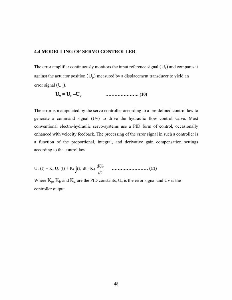
7. RESULTS AND DISCUSSION In this case Study a step signal is given as input signal. The actuator that is considered
here is a Moog electro-hydraulic actuator that is used for helicopter flight control. The
time response of a particular system is obtained in MATLAB/SIMULINK software with
the help of a scope block. The time response of a system is the behavior of the system
with respect to time. The time response is a significant parameter for evaluating the
system performance. Time response is a plot between time on X axis and Amplitude on Y
axis. The time response of an actuator, which is used in helicopter flight control system,
should be high for effective flight Control of the helicopter. As shown in Figures the
models of the hydraulic actuator, servo valve, servo controller, piston chambers and
pressure supply were made in MATLAB/SIMULINK software.
In the top level diagram actuator model shown in figure 6.1 a scope block is
connected to obtain the time response of the system. Figure 7.1 shows the time response
of the Actuator. The actuator system attains the maximum amplitude in 0.4 seconds
(approx).The time response graph that is obtained in the scope represents a satisfactory
compromise between rise time and overshoot. This time response graph, which is
obtained, is compared with the experimental time response graphs of Moog electro-
hydraulic actuator, which are shown in figure 7.6, and both the graphs were found to be
in good compromise.
In the chamber ‘A’ model which is shown in figure 6.4 a scope block is
connected to obtain the time response of the system Figure 7.2 shows the time response
of the actuator. In the simulation time response graph of the chamber ‘A’ model the
system attains the peak value in a very short period of time 0.2 seconds (approx) and
attains the minimum position in 0.4 seconds (approx). The system rises again in
amplitude and tends to attain the stable condition. The figure 7.7 shows the experimental
time response of Moog actuator. The experimental and the simulation graphs were found
to be in satisfactory compromise.
59

Figure 6.5 shows the MATLAB/SIMULINK model of the chamber ‘B’ subsystem. A
Scope block, which is shown in SIMULINK model, helps to find the time response of the
chamber ‘B’. In the simulation graph which is shown in the figure 7.3 is almost
symmetrical to the time response of chamber ‘A’. Slight asymmetry results from the
change in chamber volumes as the piston is displaced to its new position. The figure 7.7
shows the experimental time response of Moog actuator. The experimental and the
simulation graphs were found to be in satisfactory compromise.
Figure 6.2 shows the MATLAB/SIMULINK model of the actuator
subsystem. A scope block, which is shown in SIMULINK model, helps to find the time
response of the actuator for a ramp input. The figure 7.4 shows the time response of the
actuator. The sharp rising and falling edges and minimal overshoot represent the
optimum response.
.
Figure 6.3 shows the MATLAB/SIMULINK model of the servo valve
subsystem. A scope block, which is shown in SIMULINK model, helps to find the time
response of the servo valve. The figure 7.5 shows the response of the servo valve. The
system rises to maximum amplitude in 0.15 seconds (approx) and then reduces to a
minimum value of amplitude in 0.4 seconds and again the amplitude of the system
increases in magnitude and at 0.8 seconds the system tends to attain stable condition.
60
Figure 7.1 Time Response of the Linear Hydraulic Actuator
Time in seconds on Xaxis
Amplitude on Yaxis
61

Figure 7.2 Time Response of the Piston Chamber’ A’ of the Actuator
Time in seconds on Xaxis
Amplitude on Yaxis
62

Figure 7.3 Time Response of the Piston Chamber’B’ of the Actuator
Time in seconds on Xaxis
Amplitude on Yaxis
63

Figure 7.4 Time Response of the Actuator
Time in seconds on Xaxis
Amplitude on Yaxis
64

Figure 7.5 Time Response of the Servo Valve
Time in seconds on Xaxis
Amplitude on Yaxis
65

Figure7.6 Experimental time response graph of a hydraulic linear actuator (Courtesy Flight Test Centre, RWRDC)
66

Figure 7.7 experimental time response in chambers A and B (courtesy Flight Test
centre, RWRDC)
67

8. CONCLUSIONS
Mathematical models have been developed for the hydraulic system components like
hydraulic actuator, servo valve, piston chambers, and servo controllers by considering the
system requirements, system characteristics, fluid flow properties. By using these
mathematical models
MATLAB/SIMULINK models have been made for the hydraulic system components
.This time response is a very significant factor when the system considered is a critical
system like a flight control actuator.
1. These Simulink models of hydraulic actuator function like a virtual hydraulic
actuator where in we can obtain the behavior of the system with respect to time
without physically testing the component.
2. The time response of hydraulic actuator, servo valve is obtained from the
MATLAB/SIMULINK software.
3. With the help of these MATLAB/SIMULINK models the performance of the
hydraulic system components, sub systems like servo controller; servo valve etc
can be monitored.
4. By varying the subsystem parameters like pressure, active annulus area, stroke
length, control current etc the designer can arrive at optimum parameters of the
hydraulic actuator.
5. With the help of these MATLAB/SIMULINK models of electro hydraulic servo
actuator the time response of the hydraulic actuator can be obtained without
physically testing the actuator.
6. The time responses of the hydraulic actuator, servo valve and piston chamber are
compared with the MOOG hydraulic actuator data (courtesy Flight Test Centre,
RWRDC). The time response graphs which are obtained by this simulation of
electro-hydraulic actuator are found to be coinciding with the experimental time
response graphs of Moog electro hydraulic actuator.
68
9. SCOPE FOR FUTURE DEVELOPMENT
The Simulation of Hydraulic Actuator can also be done with the help of Softwares like
HYPNEU, SIMULATIONX etc.
1. The Simulation using MATLAB/SIMULINK can also be done for finding the
Time response of other hydraulic System components like Pump.
2. This Simulation using MATLAB/SIMULINK can also be applied for finding the
Time response of the Aircraft Flight control surfaces like Ailerons, Elevators and
Rudder etc.
3. The Time response of the Aircraft wheel brake System can also be obtained by
using this approach of MATLAB/SIMULINK Simulation
4. Using this approach of MATLAB/SIMULINK Simulation can also be done for
finding the Time response of Aircraft Landing Gear.
5. By this approach of simulation the behavior of the Rotary Hydraulic Actuator
with respect to time can be found out.
69
10. REFERENCES
1. Joshi, A. and Pramodh, Modelling and Simulation of Launch Vehicle Digital
Autopilot, AIAA Paper No. 4696, Proc. Of .Modeling and Simulation
Technologies Conference, Monterey, CA, USA, 6-8 August 2002
2. E. Papadopoulos, a systematic methodology for optimal component selection of
Electro hydraulic servosystems International journal of fluid power, volume 5
number 3,November 2004 page 31-39.
3. Edson Roberto, design and experimental evaluation of position controllers for
hydraulic actuators: backstepping and LQR-2DOF controllers International
journal of fluid power, volume 5, number 3, November 2004 ,page 41-53.
4. Kexiangwei, Fluid Power Control Unit Using Electro rheological Fluids,
International journal of fluid power, volume 5, number 3, November 2004,
page61-69.
5. Holger Berndt, Interactive Design and Simulation Platform for Flight Vehicle
Systems Development, IEEE Transactions on Control Systems Technology, Vol.
12, No. 2,March 2004, pp. 250–262.
6. Joshi, A. and Jayan, P.G., Modelling and Simulation of Aircraft Hydraulic System,
AIAA Paper No. AIAA-2002-4611, Proc. of Modelling and Simulation
Technologies Conference, Monterey, CA, USA, 6-8 August 2002.
7. Randall T. Anderson Mathematical Modeling of a Two Spool Flow Control
Servovalve Using a Pressure Control Pilot, ASME journal, volume 124,
September 2004.
70

8. Ashok joshi ,Modelling of Flight Control Hydraulic Actuators Considering Real
System Effects,journal of AIAA , volume 132, march 2003, pp. 123-140.
9. Peter Rowland, M. Longvitt modular design approach for modeling of large and
complex hydraulic systems ,International journal of fluid power, volume 12,
number 4,August 2005, pp 134-152.
10. Sreeraj P.N, simulation work for typical aircraft’s steering system and wheel brake
system, journal of AIAA, volume 121, November2001, pp. 153-172.
11. Panagiotis , detailed model of an electro hydraulic servo system International
journal of fluid power, volume 5, number 2,september 2004, pp 121-138.
12. Ing T.Hong, Dynamic analysis for calculating hydraulic system response, Moog
Technical Bulletin132, November 1975.
13. Paul J.Heney, challenges in aircraft hydraulic system, Moog Technical
Bulletin142, August 1978.
14. Ming Yuan –Tsuei, application of computer programs for system design and
analysis,International journal of fluid power, volume 7, number 4, September 2005,
pp.143-158. .
15. P.Krus, A.Jansson, computer simulation for optimization of hydraulic components,
International journal of fluid power, volume 12, number 4, November2005,
pp162-183.
16. Joseph N.Demarchi, development of aircraft light weight hydraulic systems, journal
of AIAA, volume 113, Dec 2001, pp. 123-132.
17. Jk Kapur, Mathematical Modeling,Prentice -Hall, New Delhi, 1993.
18. Yeaple, F, Fluid Power design Handbook, Marcel Decker, New York, 1995.
71
19. Electro hydraulic Valves a Technical Look, Moog Technical Paper 20. Moog 760 Series Servo valves, product datasheet. 21.R.H.Maskrey and W.J.Thayer,a Brief History of Electro hydraulic Servomechanisms,
Moog Technical Bulletin 141, June 1978.
22. T. P. Neal, Performance Estimation for Electro hydraulic Control Systems, Moog
Technical Bulletin126, November 1974
23. W.J.Thayer, Transfer Functions for Moog Servo valves, Moog Technical Bulletin
103, January 1965.
24. J.C.Jones, Developments in Design of Electro hydraulic Control Valves, Moog
Technical Paper, November 1997
25. D.C.Clarke, Selection & Performance Criteria for Electro hydraulic Servo valves, October1969. 26. DeRose, the Expanding Proportional and Servo Valve Marketplace, Fluid Power
Journal, March/April 2003.
27. A Systematic Methodology for Optimal Component Selection of Electro hydraulic
Servo Systems, International Journal of Fluid Power, volume 5, Nov 2004.
29. D. Caputo, Digital Motion Control for Position and Force Loops NFPA Technical
Paper I96-11.1, April 1996.
30. Beard R W, Mc Lain T W, Non linear optimal control design of a missile autopilot,
AIAA .98-4321, (1998), pp. 1209-1214.
72

31. Greensite.A, Analysis and design of space vehicle control systems, Spartan Books,
NewYork, 1970.
32. Greensite.A, Elements of modern control theory, Spartan Books, New York, 1970. 33. Stringer, J.D., Hydraulic Systems Analysis, the Macmillan Press Ltd., 2nd Edition,1982. 34. Guillon M, Hydraulic Servo Systems Analysis and Design, Butterworth & Co Ltd., 1969. 35. Viersma, T. J., Analysis, Synthesis and Design of Hydraulic Servosystems and
Pipelines, Elsevier Scientific Publishing Company, 1980.
36. Walter, R. B., Hydraulic and Electro hydraulic Control system, Cliff, London, 1967.
37. Merritt, Herbert E., 1967, Hydraulic Control Systems, Wiley, New York.
73