simulated annealing - iit madras cse dept.vplab/courses/optimization/sa_sel_slides.pdf · annealing...
TRANSCRIPT


Simulated Annealing

Hill climbing

Simulated AnnealingLocal Search
Solution space
Cos
t fun
ctio
n
?

Annealing Annealing is a thermal process for obtaining low energy states of a solid
in a heat bath.
The process contains two steps: Increase the temperature of the heat bath to a maximum value at which the solid
melts. Decrease carefully the temperature of the heat bath until the particles arrange
themselves in the ground state of the solid. Ground state is a minimum energy state of the solid.
The ground state of the solid is obtained only if the maximum temperature is high enough and the cooling is done slowly.


Simulated Annealing To apply simulated annealing with optimization purposes we require the following:
A successor function that returns a “close” neighboring solution given the actual one. This will work as the “disturbance” for the particles of the system.
A target function to optimize that depends on the current state of the system. This function will work as the energy of the system.
The search is started with a randomized state. In a polling loop we will move to neighboring states always accepting the moves that decrease the energy while only accepting bad moves accordingly to a probability distribution dependent on the “temperature” of the system.

Simulated Annealing
The distribution used to decide if we accept a bad movement is know as Boltzman distribution.
Decrease the temperature slowly, accepting less bad moves at each temperature level until at very low temperatures the algorithm becomes a greedy hill-climbing algorithm.
This distribution is very well known is in solid physics and plays a central role in simulated annealing. Where γ is the current configuration of the system, E γ is the energy related with it, and Z is a normalization constant.

Annealing Process• Annealing Process
– Raising the temperature up to a very high level (melting temperature, for example), the atoms have a higher energy state and a high possibility to re-arrange the crystallinestructure.
– Cooling down slowly, the atoms have a lower and lower energy state and a smaller and smaller possibility to re-arrange the crystalline structure.

Statistical Mechanics
Combinatorial Optimization
State {r:} (configuration -- a set of atomic position )
weight e-E({r:])/K BT -- Boltzmann distribution
E({r:]): energy of configuration
KB: Boltzmann constant
T: temperature
Low temperature limit ??

AnalogyPhysical System
State (configuration)
Energy
Ground State
Rapid Quenching
Careful Annealing
Optimization Problem
Solution
Cost function
Optimal solution
Iteration improvement
Simulated annealing

Simulated Annealing• Analogy
– Metal Problem– Energy State Cost Function– Temperature Control Parameter– A completely ordered crystalline structure the optimal solution for the problem
Global optimal solution can be achieved as long as the cooling process is slow enough.
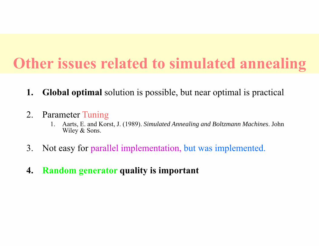
Other issues related to simulated annealing
1. Global optimal solution is possible, but near optimal is practical
2. Parameter Tuning1. Aarts, E. and Korst, J. (1989). Simulated Annealing and Boltzmann Machines. John
Wiley & Sons.
3. Not easy for parallel implementation, but was implemented.
4. Random generator quality is important

Analogy
• Slowly cool down a heated solid, so that all particles arrange in the ground energy state
• At each temperature wait until the solid reaches its thermal equilibrium
• Probability of being in a state with energy E :
Pr { E = E } = 1 / Z(T) . exp (-E / kB.T)
E EnergyT TemperaturekB Boltzmann constantZ(T) Normalization factor (temperature dependant)

Simulated Annealing• Same algorithm can be used for combinatorial optimization problems:• Energy E corresponds to the Cost function C• Temperature T corresponds to control parameter c
Pr { configuration = i } = 1/Q(c) . exp (-C(i) / c)
C Costc Control parameterQ(c) Normalization factor (not important)

Components of Simulated Annealing
• Definition of solution
• Search mechanism, i.e. the definition of a neighborhood
• Cost-function

Control Parameters
1. Definition of equilibrium1. Definition is reached when we cannot yield any significant
improvement after certain number of loops2. A constant number of loops is assumed to reach the equilibrium
2. Annealing schedule (i.e. How to reduce the temperature)1. A constant value is subtracted to get new temperature, T’ = T - Td2. A constant scale factor is used to get new temperature, T’= T * Rd
• A scale factor usually can achieve better performance
1. How to define equilibrium?
2. How to calculate new temperature for next step?
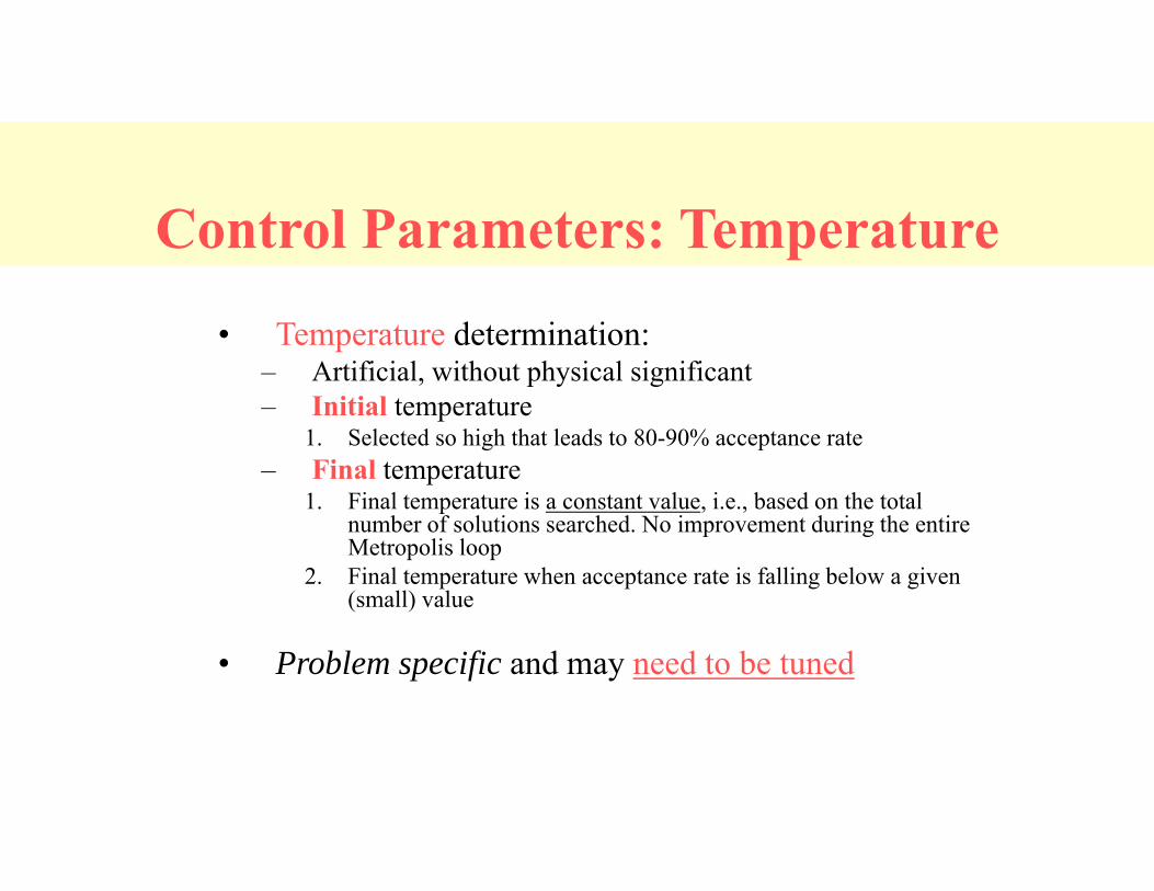
Control Parameters: Temperature
• Temperature determination:– Artificial, without physical significant– Initial temperature
1. Selected so high that leads to 80-90% acceptance rate– Final temperature
1. Final temperature is a constant value, i.e., based on the total number of solutions searched. No improvement during the entire Metropolis loop
2. Final temperature when acceptance rate is falling below a given (small) value
• Problem specific and may need to be tuned

Simulated Annealing: the code1. Create random initial solution γ2. Eold=cost(γ);3. for(temp=tempmax; temp>=tempmin;temp=next_temp(temp) ) {4. for(i=0;i<imax; i++ ) {5. succesor_func(γ); //this is a randomized function6. Enew=cost(γ);7. delta=Enew-Eold;8. if(delta>0)9. if(random() >= exp(-delta/K*temp);10. undo_func(γ); //rejected bad move11. else12. Eold=Enew //accepted bad move13. else14. Eold=Enew; //always accept good moves
}}

Simulated Annealing Acceptance criterion and cooling schedule

Practical Issues with simulated annealing Cost function must be carefully developed, it has to
be “fractal and smooth”. The energy function of the left would work with SA
while the one of the right would fail.

Practical Issues with simulated annealing The cost function should be fast it is going to be called
“millions” of times. The best is if we just have to calculate the deltas produced by
the modification instead of traversing through all the state. This is dependent on the application.

Practical Issues with simulated annealing In asymptotic convergence simulated annealing converges to
globally optimal solutions. In practice, the convergence of the algorithm depends of the
cooling schedule. There are some suggestion about the cooling schedule but it
stills requires a lot of testing and it usually depends on the application.

Practical Issues with simulated annealing Start at a temperature where 50% of bad moves are accepted. Each cooling step reduces the temperature by 10% The number of iterations at each temperature should attempt to move
between 1-10 times each “element” of the state. The final temperature should not accept bad moves; this step is known
as the quenching step.

Applications Basic Problems
Traveling salesman Graph partitioning Matching problems Graph coloring Scheduling
Engineering VLSI design
Placement Routing Array logic minimization Layout
Facilities layout Image processing Code design in information theory

Example of Simulated Annealing
• Traveling Salesman Problem (TSP)– Given 6 cities and the traveling cost between
any two cities– A salesman need to start from city 1 and travel
all other cities then back to city 1– Minimize the total traveling cost

Example: SA for traveling salesman
• Solution representation– An integer list, i.e., (1,4,2,3,6,5)
• Search mechanism– Swap any two integers (except for the first one)
• (1,4,2,3,6,5) (1,4,3,2,6,5)
• Cost function

• Temperature1. Initial temperature determination
1. Initial temperature is set at such value that there is around 80% acceptation rate for “bad move”
2. Determine acceptable value for (Cnew – Cold)2. Final temperature determination
• Stop criteria• Solution space coverage rate
Example: SA for traveling salesman
• Annealing schedule (i.e. How to reduce the temperature)
– A constant value is subtracted to get new temperature, T’ = T – Td
– For instance new value is 90% of previous value.
• Depending on solution space coverage rate


Simulated Annealing The process of annealing can be simulated with the Metropolis
algorithm, which is based on Monte Carlo techniques. We can apply this algorithm to generate a solution to combinatorial
optimization problems assuming an analogy between them and physical many-particle systems with the following equivalences: Solutions in the problem are equivalent to states in a physical system. The cost of a solution is equivalent to the “energy” of a state.

Simulated Annealing Algorithm
Initialize:– initial solution x , – highest temperature Th, – and coolest temperature Tl
T= ThWhen the temperature is higher than Tl
While not in equilibriumSearch for the new solution X’Accept or reject X’ according to Metropolis Criterion
EndDecrease the temperature T
End