Simulating Flow Level Bandwidth Sharing with Paretodistributed File Sizes

Julio Rojas-Mora and Tania JiménezLIA, University of Avignon,

339, chemin des Meinajaries, Agroparc BP1228, 84911 Avignon Cedex 9, France.

Eitan AltmanMaestro group, INRIA,

2004 Route des Lucioles, 06902 SophiaAntipolis Cedex, France.eitan.altman@inria.fr

ABSTRACTOur goal is to achieve deeper understanding of the limita-tion of queueing models, on one hand, and of common sim-ulation practice, on the other hand, as tools for predictingperformance of bandwidth sharing between competing TCPflows. In particular, we (i) present an overview of simulationproblems that are expected to arise due to the very heavytail of the distribution of the size of TCP flows, and (ii)through simulations we show that the average sojourn timeof competing flows are quite sensitive to various networkparameters. The understanding that we get from the firstpoint allows us to better assess when are the conclusionsfrom simulation results on bandwidth sharing reliable.

Using simulations in ns2, we study bandwidth sharing un-der various load factors and show the benefit of using boot-strap as a post simulation tool for analyzing the simulationresults.

KeywordsM/G/1 queue. Processor Sharing. Simulation. Confidenceinterval.

1. INTRODUCTIONIn this paper we present a short overview of difficulties in

the evaluation of bandwidth sharing of TCP flows. We firstpresent an overview on the limitations of analytical toolsbased on flow level queueing models. We then highlight thedifficulties in a simulation based approach.

The processor sharing queue has been perhaps the mostcommon model for bandwidth sharing of flows (having thesame RTT) of data transfer over the Internet [4], along withthe Discriminatory Processor Sharing queue [7] adapted tothe case of unequal round trip times. Several research groupshave examined its validity through simulations [17, 14, 11,13]. The conclusions of the papers have not always beenencouraging. Indeed,

• Some papers support the modeling of flow level band-width sharing through PS queues but find a gap be-

Permission to make digital or hard copies of all or part of this work forpersonal or classroom use is granted without fee provided that copies arenot made or distributed for profit or commercial advantage and that copiesbear this notice and the full citation on the first page. To copy otherwise, torepublish, to post on servers or to redistribute to lists, requires prior specificpermission and/or a fee.Copyright 20XX ACM X-XXXXX-XX-X/XX/XX ...$10.00.

tween the predicted PS model and the simulated model.For example, in [11] the authors write: “We find thatthe average bandwidth share from our model is closeto that obtained from a Processor Sharing (PS) modelassuming that the link speed is 75% of the actual linkspeed.”

• In some papers the idea of using a processor sharingtype model is criticized. An example is [14] who studyprocessor sharing models in overload. The differencesbetween the simulation and the model’s predicted per-formance goes up to an order of magnitude.

• A more refined model is presented in [23] with anM/G/R PS queue: in that model, the flows do notinteract with each other, and the rate at which thepackets of each flow are served is not influenced bythe number of flows as long as their number is smallerthan R. Only when their number exceeds R, the totalcapacity of the R servers is split equally among theflows. For a small size of flows, it is found that themodel underestimates the simulations by a factor ofthree.

The fact that different contradicting findings have ap-peared on bandwidth sharing among competing Internetflows can be due either to shortcoming related to simula-tions and to their interpretation, or to shortcoming in themodeling. As an example for the first possibility, we wouldcite the authors of [11] who write concerning the heavy taildistribution of the file sizes on the internet: “since a substan-tial part of the distribution is in the tail, if the simulationis not run for very long the average of the sampled file sizeswould be less than the nominal average, thus leading to alower offered load and hence overestimation of the through-put.”

In order to understand the shortcoming of the processorsharing queue as a model for bandwidth sharing we need firstto be able to obtain reliable comparisons to simulations orto real measurements. For that, we need to accompany sim-ulations with estimation of the confidence interval. The cen-tral limit based confidence intervals may be quite misleadingor non-informative as the second moment of the number offlows or of the workload in the system are infinite in station-ary regime. We apply therefore an alternative approach toderive confidence intervals and use bootstrap which allowsone to obtain more accurate estimation of the confidenceintervals and at the same time allows one to accelerate thesimulations.

2. BACKGROUND AND RELATED WORK

In the following subsection we present a brief overviewof queueing based modeling of bandwidth sharing. Theyinclude various papers that identified bad fit when comparedto simulations. The simulations themselves to which thesemodels are compared may be unreliable due to the heavytailed distribution of the flow sizes; this is discussed in thefollowing subsection. We then state the contribution of thispaper.

2.1 Modeling bandwidth sharing using proces-sor sharing type queueing models

We have found both good as well as bad fit between theprocessor sharing prediction for computing the sojourn timesand the values obtained by simulations. An extreme exam-ple is [13] where an entire order of magnitude of difference isreported between the two. Much better fitness is obtainedin some other such as [11], where the differences are of theorder of 10%.

2.1.1 Overload conditionsIn [14] the authors study a link during a transient overload

with TCP connections. (Overload occurs during periods atwhich the capacity of the bottleneck link is lower than therate at which new data is generated for connections that usethe bottleneck. More precisely, if new flows that use thebottleneck keep arriving at a given rate, say λ per second,and a flow average size (including overheads such as head-ers) is s, then overload occurs if the bottleneck’s capacity islower than λs.) They consider the case where user behaviordoesn’t change with congestion, i.e., transfers are neither in-terrupted nor reattempted. In first place they observe thatfor different distributions of the size of the transferred file,the number of concurrent connections to the link after con-gestion starts, grows linearly in time and their slope growsinversely with variance. This behavior is also seen in therate in which the number of concurrent ongoing flows grows.Comparisons with the PS model show that TCP simulationsgive much higher growth rates. This is explained by packetretransmissions which affects the effective offered load, andwhich are not modeled by the PS model.

In PS the increase rate of population overload is knownto be sensitive to the distribution of the arrival processonly through its mean. The authors show however thatthere is some effect of the inter-arrival times distribution inTCP concurrent connections growth rate, with worst per-formances given by distributions with higher variances. Theauthors say that this behavior can be explained by the slowerservice rate of transfers arriving in bursts, which stay longerin the system.

It is also observed that for normalized sojourn time, TCPperformance degrades at least an order of magnitude fasterthan PS when files grow in size. This ratio remains constantfor all sizes evaluated, thus long connections are as affectedas short ones.

For short connections, it is seen for those smaller than3 packets (packets of 1500 bytes) that sojourn times con-verge very fast in median to less than 0.5 seconds, but 90%of the connections are below 3 seconds. For slightly largerconnections (between 4 and 15 packets), the median is ap-proximately 2.5 seconds while the 90th percentile is morethan 15 seconds. This shows that short connections thattake long to finish should be restarted as they will finishfaster this way.

In the PS model, the normalized transfer time tends toa deterministic limit that grows exponentially in the size ofthe file transferred. In this paper, simulations show thateven after one hour of congestion normalized transfer timesare far from converging, with very high variability speciallyin small connections. This means that small transfers donot take advantage of their size to finish before longer onesas they do in a PS queue. The authors feel that reducingthe dispersion of transfer times will improve performance,specially for short connections.

2.1.2 Other modelsThe M/G/R PS model is used in [23] to study the sojourn

time as a function of the file size for one fixed value of RTT.This model underestimates the results of simulations by aquantity that remains quite constant as the size of the filegrows. The relative error is seen to be obtained when thesize of the file is the smallest. In particular, for the smallestfile size considered, the authors find that the model under-estimates the simulations by a factor of three.

In [17] the authors consider non symmetric RTTs. Theydevelop a DPS (Discriminatory Processor Sharing) queuemodel for TPC in the overload regime and test it with sim-ulations in ns2. They obtain an agreement between the ex-pected and the simulated result (with an error of around10%).

2.2 Simulation involving flows with heavy tailedsize distribution

The expected sojourn time of a customer in a processorsharing queue is known to be insensitive to the file size dis-tribution (it depends on the distribution only through theexpectation). Its variance, however, is not insensitive any-more, and in particular, it is infinite when the service timeof a client (or equivalently in our setting - the size of a filethat is transferred) has an infinite second moment [3].

The size of a data transfer over the Internet is knownto be heavy tailed [12]. (This is the case for both FTPtransfers as well as for the “on” periods of HTTP transfers).Among several candidates for modeling the distribution ofthese transfers, the Pareto distribution with parameter be-tween 1.05 and 1.5 has been the one that gave the best fitwith experiments for the last twenty years, see [8, 2, 6, 15].

This very heavy tail has been causing various serious prob-lems for simulations of data transfers.

An important problem is in the reliability of the results.Standard approach to assess it involve the central limit basedconfidence intervals. However, this approach is not directlyapplicable whenever the variance is infinite, which is thecase with the stationary sojourn time of a data transfer flow(having a Pareto distribution with a shape parameter Klower than 2). A second problem is the very long durationof simulations needed in order to get good precision.

We present a brief overview of simulation problems en-countered in the context of bandwidth sharing among TCPflows

• The authors of [11] write: “since a substantial part ofthe distribution is in the tail, if the simulation is notrun for very long the average of the sampled file sizeswould be less than the nominal average, thus leadingto a lower offered load and hence overestimation of thethroughput.”

• Due to the last points one may have problems in inter-

pretation of simulation results . Indeed, various papersin which sharing bandwidth is modeled by processorsharing report differences between the expected theo-retical value and the simulation value [13, 14, 11, 17]that vary from around 10% in [11] and go up to a factorof 10 in some situations in [13]. When such deviationsoccur, it is important to know whether they can bedue to the imprecisions in the simulation or to realphenomena.

• The warm-up time is extremely long, see [9].

• One way to avoid heavy tails is to truncate them. Thisis in spirit of the suggestion in the paper “Difficul-ties in simulating queues with Pareto service” [10] thatsays: “Since for any finite simulation run length, thereis always a maximum value of the random variablesgenerated, we, in actuality, are simulating a truncatedPareto service distribution. It has also been argued thatthere is always a maximum file size or claim amountso, in reality, we are always dealing with truncated dis-tributions.” But where should we truncate the distri-bution? Truncation at some size M would be valid ifthe difference between performance with truncation atany other value L that is greater than M has a negli-gible impact on performance. Simulating with a trun-cated Pareto distribution may not be sufficient andseveral other tests of truncation at larger thresholdvalues may be needed. Other approaches are to ap-proximate Pareto with Lognormal or to treat the datafrom heavy-tailed simulations as transient [24].

2.3 Our contributionsWe have presented the background and the work related

to the use of processor sharing queues to model bandwidthsharing at the Internet on the flow level. We have putforward the disagreements and the debate related to thatmodel. We also summarized the difficulties in simulatingor in interpreting the simulation results due to the heavytail nature of Internet traffic. The contributions of this pa-per are first in proposing and testing statistical methods forpreprocessing the simulation results that have not been usedmuch in networking. Indeed,

• Confidence Intervals : We use the quantile basedapproach as an alternative to the central limit basedapproach for obtaining the confidence intervals. Thecentral limit approach is not directly applicable when-ever the variance is infinite, which is the case withthe stationary sojourn time of a data transfer session(having a Pareto distribution with a shape parameterK lower than 2).

• We then apply this approach directly to the simulationof competing non-persistent TCP transfers of files thathave heavy tail distribution. We compare the simula-tion results to those obtained for the processor sharingqueue. We identify various reasons for the deviation ofthe behavior of TCP from the ideal processor sharingmodel and manage to quantify the impact of some ofthese.

Structure of the paperIn Section 3 we present our approach concerning the useof simulation to estimate the average number of packets in

the processor sharing queue. We then present in Section 4simulations of TCP connections that share a common bot-tleneck link and compare the precision that can be obtained(with and without the bootstrap approach) to the precisionobtained in simulating the processor sharing queue. We pro-vide explanations for the differences between the TCP sce-nario and its corresponding processor sharing model. A con-cluding section summarizes the paper. An appendix presentssome background on Bootstrap and on quantile based con-fidence intervals.

3. SIMULATING THE QUEUE SIZE OF APROCESSOR SHARING QUEUE

Through a series of simulations performed in JAVA (avail-able from the authors by request) we exhibit the power ofthe bootstrap approach: its ability to increase the precisionof the simulation of Internet traffic that is throttled by somebottleneck link and at the same time decrease the requiredduration of the simulation. In this section we restrict our-selves to study of the processor sharing queue which hadoften been proposed as a model for TCP transfers sharing abottleneck link in the Internet. A TCP flow is then repre-sented by one customer in the PS queue.

Below we used the PS queue with a Poisson arrival pro-cess with a rate of λ = 1 customers per second. (A customerrepresents a file when the processor sharing queue is used tomodel file transfers). We consider three service time dis-tributions: Pareto with shape parameter 1.5, Pareto withshape 2.5, and exponentially distributed. We vary the aver-age service time σ so as to obtain an average load ρ = λσthat takes the values 0.6 and 0.7.

Each one of the figures below correspond to the queuesize of the processor sharing averaging over 100 independentsamples. When considering the PS queue as a model forbandwidth sharing in the Internet, the queue size should beinterpreted as the number of ongoing flows.

The duration of each simulation is 6·106 sec and there isa warm up time of 300000 sec. In each one of the scenariosdescribed in Figure 1, we present:

1. the theoretical steady state expected queue size

2. the value obtained by the simulations

3. the confidence interval corresponding to a 95% per-centile, obtained using the quantile method, and

4. the confidence intervals corresponding to a 95% confi-dence level after applying the bootstrap method.

We took 100000 resamples out of our 100 original samplesfor the bootstrap.

Figure 1 displays the precision of the simulations withand without the bootstrap approach for ρ = 0.6 (up) andρ = 0.7 (down). The left subfigures are for an exponentialdistributed service time, the middle and right ones are for aPareto distributed service time with parameter K = 2.5 andK = 1.5, respectively. The average service time is the samein the all three sub-figures corresponding to the same ρ. (Itwas chosen so that indeed ρ = λ · σ will have the values 0.6and 0.7, respectively.)

We observe the following points from the simulations:

• The simulations show well the insensitivity of the PSregime to the service time distribution. Indeed, in each

1e+06 3e+06 5e+06

1.46

1.48

1.50

1.52

1.54

Arrivals

Ave

rage

Ses

sion

s

TheoryEstim.Perc. CIBoot. CI

1e+06 3e+06 5e+06

1.46

1.48

1.50

1.52

1.54

Arrivals

Ave

rage

Ses

sion

s

TheoryEstim.Perc. CIBoot. CI

1e+06 3e+06 5e+06

1.4

1.6

1.8

2.0

Arrivals

Ave

rage

Ses

sion

s

TheoryEstim.Perc. CIBoot. CI

1e+06 3e+06 5e+06

2.25

2.30

2.35

2.40

Arrivals

Ave

rage

Ses

sion

s

TheoryEstim.Perc. CIBoot. CI

1e+06 3e+06 5e+06

2.25

2.30

2.35

2.40

Arrivals

Ave

rage

Ses

sion

s

TheoryEstim.Perc. CIBoot. CI

1e+06 3e+06 5e+06

2.2

2.4

2.6

2.8

3.0

3.2

3.4

Arrivals

Ave

rage

Ses

sion

s

TheoryEstim.Perc. CIBoot. CI

Figure 1: Average number of flows with ρ = 0.6 (up) and ρ = 0.7 (down). Exponential distribution (left) andPareto distribution with parameter K = 2.5 (middle) and K = 1.5 (right)

set of simulations having the same load ρ, we see con-vergence to the same average rate for the exponentialcase, the Pareto distribution with parameter K = 2.5and for the Pareto distribution with K = 1.5.

• The 95% confidence interval without bootstrap is around10 times larger than that of the bootstrap (which es-tablishes clearly the advantage of using it). This isseen to hold for any duration of the simulation.

• We see that the confidence interval are around 10 timessmaller in the case of exponential and Pareto withshape parameter of 2.5 than in the case of Pareto shapeparameter 1.5. This can be expected since the tail ofthe latter distribution is much heavier.

• Duration of the simulation: For all three distributions,and for the different loads, we see that the precisionobtained with bootstrap after already 400000 sec ismore than three times better than that without boot-strap after we see that even after 6 million seconds.It thus seems that to get the same precision withoutbootstrap, one would need to use simulations muchlonger than 15 times as much as with bootstrap.

4. SIMULATING TCP CONNECTIONSWe compare in this section simulations that we performed

with ns2.33 of TCP flows with the simulation of the pro-cessor sharing queue. The network we simulate is given inFigure 2.

Figure 2: Network Topology

We took 200 input links, each of speed 100 Mbps. Thepacket size was taken to be 1 KByte. The average flow sizewas taken to be 200 KBytes. The total round trip delay is0.4 msec. We simulate the New Reno version without thedelayed Ack option. The maximum window size is of 20packets, which is the default size of ns2. We later changethis value.

To make comparisons between precision of simulationsthat have different event rates and different averages, wefind it convenient to normalize the confidence interval. weused the estimated relative half-width (ERHW) of the con-fidence interval defined as half the difference between theupper and the lower values of the interval divided by theaverage value.

4.1 Bootstrap and the confidence intervalWe are interested in comparing confidence intervals ob-

tained with bootstrap when simulating a processor sharingqueue, on one hand, and when simulating TCP, on the other

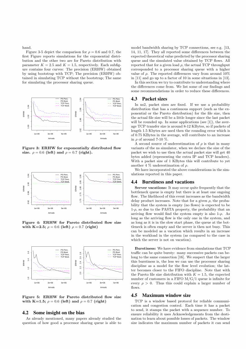
hand.Figure 3-5 depict the comparison for ρ = 0.6 and 0.7, the

first Figure reports simulations for the exponential distri-bution and the other two are for Pareto distribution withparameter K = 2.5 and K = 1.5, respectively. Each subfig-ure contains four curves: The precision (ERHW) obtainedby using bootstrap with TCP; The precision (ERHW) ob-tained in simulating TCP without the bootstrap; The samefor simulating the processor sharing queue.

1e+06 3e+06 5e+06

1.00

1.02

1.04

Arrivals

ER

HW

PS Perc.PS Boot.TCP Perc.TCP Boot.

1e+06 3e+06 5e+06

1.82

1.86

1.90

1.94

Arrivals

ER

HW

PS Perc.PS Boot.TCP Perc.TCP Boot.

Figure 3: ERHW for exponentially distributed flowsize. ρ = 0.6 (left) and ρ = 0.7 (right).

1e+06 3e+06 5e+06

0.92

0.96

1.00

1.04

Arrivals

ER

HW

PS Perc.PS Boot.TCP Perc.TCP Boot.

1e+06 3e+06 5e+06

1.70

1.75

1.80

1.85

1.90

Arrivals

ER

HW

PS Perc.PS Boot.TCP Perc.TCP Boot.

Figure 4: ERHW for Pareto distributed flow sizewith K=2.5; ρ = 0.6 (left) ρ = 0.7 (right)

1e+06 3e+06 5e+06

1.0

1.2

1.4

1.6

Arrivals

ER

HW

PS Perc.PS Boot.TCP Perc.TCP Boot.

1e+06 3e+06 5e+06

2.0

2.2

2.4

2.6

2.8

Arrivals

ER

HW

PS Perc.PS Boot.TCP Perc.TCP Boot.

Figure 5: ERHW for Pareto distributed flow sizewith K=1.5; ρ = 0.6 (left) and ρ = 0.7 (right)

4.2 Some insight on the biasAs already mentioned, many papers already studied the

question of how good a processor sharing queue is able to

model bandwidth sharing by TCP connections, see e.g. [13,14, 11, 17]. They all reported some differences between theexpected theoretical value predicted by the processor sharingqueue and the simulated value obtained by TCP flows. Allreported that for a given load ρ, the actual TCP throughputcorresponded to a processor sharing queue with a highervalue of ρ. The reported differences vary from around 10%in [11] and go up to a factor of 10 in some situations in [13].

In this section we try to contribute to understanding wherethe differences come from. We list some of our findings andsome recommendations in order to reduce these differences.

4.3 Packet sizesIn ns2, packet sizes are fixed. If we use a probability

distribution that has a continuous support (such as the ex-ponential or the Pareto distribution) for the file size, thenthe actual file size will be a little longer since the last packetwill be rounded up. In some applications (see [1]), the aver-age TCP transfer size is around 8-12 KBytes, so if packets oflength 1.5 Kbytes are used then the rounding error which isof 0.75 KBytes in the average, will contribute to an increasein ρ of around 7-10 %.

A second source of underestimation of ρ is that in manyvariants of the ns simulator, when we declare the size of thepacket we wish to use then the actual packet size will get 40bytes added (representing the extra IP and TCP headers).With a packet size of 1 KBytes this will contribute to yetanother 4 % underestimation of ρ.

We have incorporated the above considerations in the sim-ulations reported in this paper.

4.4 Burstiness and vacationsServer vacations: It may occur quite frequently that the

bottleneck queue is empty but there is at least one ongoingflow. The likelihood of this event increases as the bandwidthdelay product increases. Note that for a given ρ, the proba-bility that the system is empty (no flows) is expected to be1-ρ, so due to the PASTA property, the probability that anarriving flow would find the system empty is also 1-ρ. Aslong as the arriving flow is the only one in the system, andas long as it is in the slow start phase, the queue at the bot-tleneck is often empty and the server is then not busy. Thiscan be modeled as a vacation which results in an increasein the workload in the system (as compared to the case inwhich the server is not on vacation).

Burstiness: We have evidence from simulations that TCPtraffic can be quite bursty: many successive packets can be-long to the same connection [16]. We suspect that the largerthis burstiness is, the less we can use the processor sharingdiscipline as a model for the flow level evolution; the lat-ter becomes closer to the FIFO discipline. Note that withthe Pareto file size distribution with K = 1.5, the expectednumber of customers in a FIFO M/G/1 queue is infinite forevery ρ > 0. Thus this could explain a larger number offlows.

4.5 Maximum window sizeTCP is a window based protocol for reliable communi-

cation and congestion control. Each time it has a packetto send, it stamps the packet with a sequence number. Toensure reliability it uses Acknowledgements from the desti-nation to learn about possible losses of packets. The windowsize indicates the maximum number of packets it can send

before receiving an acknowledgement. The larger the win-dow is, the larger the transmission rate is. In absence of con-gestion (i.e. as long as Acknowledgements arrive regularlyand losses are not detected) the window size keeps growing,until it reaches a maximum size. The default value for thissize is 20 packets in ns2. The larger the maximum value is,the more we can expect the connection to be bursty, so wecan expect to a larger average number of flows as argued inSection 4.4.

1.5

2.0

2.5

3.0

3.5

2 8 14 20 40 64 100

Window Size

Ave

rage

Ses

sion

s

Figure 6: Average number of ongoing flows as afunction of the max TCP window size.

We have tested through simulations the impact of themaximum TCP window size on the expected number of on-going flows and discovered that the latter is indeed sensitiveto the maximum window size. The larger the maximumwindow size is, the larger is the average number of ongoingflows and the average transfer time of a connection. Thiscould perhaps be explained by the burstiness.

We present below our experiments on the impact of themaximum window size on the average number of active flowsas well as on other parameters.

Figure 6 reports on the empirical distribution of the aver-age number of ongoing flows as a function of the maximumTCP window size.

For each value of maximum window size, we did 20 simu-lations. Each simulation lasted till 2000000 arrivals of flowsoccurred. The 600000 first flows were ignored (this was thewarm up time). The other parameters of the simulations areas in Section 4.1.

For each value of maximum window size, we give the em-pirical probability density of the average number of flows.This is described by the contour of the beanplots (that rep-resents the histogram). Each white bar inside a beanplotrepresents the average size in one of the twenty simulations.The black bar that traverses each one of the beanplot givesthe average obtained from the set of 20 simulations. Thedotted horizontal line gives the theoretical average numberof customers in the corresponding processor sharing queue.

As we can see, the expected number of ongoing TCP flowsthat fully agrees with the processor sharing model is the oneobtained with a maximum window size of 8. All other val-ues of maximum window size below 20 gave deviations notgreater than 10% with respect to the theoretical value. How-

2040

6080

2 8 14 20 40 64 100

Window Size

Max

. Ses

sion

s

Figure 7: Max number of ongoing flows as a functionof the max TCP window size.

0.56

0.58

0.60

0.62

2 8 14 20 40 64 100

Window Size

Ave

rage

Rho

Ses

sion

s

Figure 8: Fraction of arrivals of flows that found thesystem non-empty upon arrival

ever, we see that for a maximum size of 100, the expectednumber of flows is almost double the theoretical value.

Figure 7 reports on the empirical distribution of the max-imum number of ongoing flows that were present simultane-ously at some time during the simulation, as a function ofthe maximum TCP window size. Note that unlike the caseof average sizes, in which each sample average takes anothervalue, the number of different values of the maximum num-ber of flows that we had within our simulations takes finitelymany values, and some values appear several times duringthe simulations. The number of times that a value appearsin the simulations is represented by the length of a whiteline (and when this value is so large that the line exceedsthe boundary of the beanplot, then the bar continuous inblack).

Figures 8-9 reports on the empirical distribution of thefraction of arrivals of flows that found the system non-emptyupon arrival, and the fraction of arrivals that found the bot-tleneck queue non-empty. The difference between these in-

0.50

0.54

0.58

0.62

2 8 14 20 40 64 100

Window Size

Ave

rage

Rho

Pac

kets

Figure 9: Fraction of arrivals that found the bottle-neck queue non-empty, as a function of the maxi-mum window size.

dicate that from time to time there are no transmissions andyet there are ongoing flows. We shall return to that pointtowards the end of the section.

4.6 Buffer sizeThe buffer size at the bottleneck queue turned out to be

yet another factor that has an influence on the average num-ber of ongoing flows. With a maximum window size of 8 andwith ρ = 0.6, the size of the buffer for which we obtainedfull agreement of the average number of flows with the the-oretical value (of 1.5) given by the processor sharing was 64.However, we observe that the simulations give good approx-imations for any larger value of the buffer size, see Figures10-11. In both figures the largest value of buffer size thatwe tested was of 1 million packets. We write “INF” in thecurves for “Infinite buffer” since with the size of 1 millionwe had no packet losses, so any buffer of larger size than 1million would give the same results in this simulation.

The second of these figures uses bootstrap which is seento result in a considerably better precision.

To understand the deviations from the theoretical valuewe measure the fraction of time that the queue is empty butthere are ongoing flows. We took a maximum window sizeof 8, ρ = 0.6, K = 1.3. We obtained around 8% for the caseof buffer size of 12 packets, and 0.36% for a buffer of size 64.

We thus attribute the large deviations from the theoreti-cal value to many losses that occur and that result in largeperiods during which the queue is empty although there areongoing flows. During these times, the processor sharingqueue has “service vacations” and the theoretical results fora queue without vacation are not valid anymore.

This phenomena is countered when using a smaller valueof the window sizes and therefore in spite of small buffers onegets better agreement with theoretical results if the maxi-mum window size is smaller.

Note that the “rule of thumb” for selecting buffer size asthe bandwidth delay product would give a value of 2 packetsin our case which gives values of number of flows much largerthan the theoretical value predicted by the processor sharingqueue.

For ρ = 0.7 we obtained very similar results. The theo-retical average number of flows in a processor sharing queueis 2.33. For a maximum window size of 8 we obtained thefollowing values for the average number of flows: 7.41, 3.723and 2.423 for a buffer of size 12, 24 and 64, respectively.

5. CONCLUSIONS

1.2

1.4

1.6

1.8

2.0

2.2

2.4

LB24 LB36 LB64 LBINF

Buffer Size

Ave

rage

Ses

sion

s

Figure 10: Average number of ongoing flows as afunction of the queue size. CI are obtained by thequantile approach.

We have studied in this paper the benefits that the boot-strap method can bring to the simulations of internet trafficsharing a common bottleneck link, and more generally, ofthe processor sharing queue with heavy tailed service times,which has served as a model for TCP sharing common re-sources. We found out that due to problems which arisewhen the central limit theorem cannot be applied, the boot-strap method to calculate confidence intervals is a practicalalternative that, at the same time, has the aggregated bene-fit of substantially shortened simulations. We have analyzedthe discrepancy between the results predicted by using theprocessor sharing queue and those obtained by simulating di-rectly the short lived TCP connections that share a commonbottleneck queue. We identified various possible reasons forthe discrepancy and provided some recommendations thatcan help understand and minimize them.

AcknowledgementThe work of the last author was partly suppported by theSemnet project of the joint INRIA Alcatel-Lucent Lab.

6. REFERENCES[1] K. Thomspson, G. J. Miller, R. Wilder, “Wide area

Internet traffic patters and characteristics, IEEENetwork 6(11), 1997, pp 10-23.

[2] B. Sikdar, S. Kalyanaraman and K. S. Vastola, “AnIntegrated Model for the Latency and Steady-StateThroughput of TCP Connections”, PerformanceEvaluation, v.46, no.2-3, pp.139-154, September 2001.

[3] T. J. Ott, “The Sojourn-Time Distribution in theM/G/1 Queue with Processor Sharing”, Journal ofApplied Probability, Vol. 21, No. 2 (Jun., 1984), pp.360-378

[4] J.W. Roberts, “A survey on statistical bandwidthsharing”. Computer Networks 45, 319-332 (2004).

[5] K. Tutschku and Ph. Tran-Gia, “Traffic characteristicsand performance evaluation of Peer-to-Peer systems”.In: Steinmetz, R., Wehrle, K. (eds.) Peer-to-PeerSystems and Applications. LNCS, pp. 383-397.Springer, Heidelberg (2005)

1.4

1.6

1.8

2.0

2.2

24 36 64 INF

Buffer Size

Ave

rage

Ses

sion

s

Figure 11: Average number of ongoing flows as afunction of the queue size. CI are obtained from thebootstrap.

[6] P. Olivier, “Internet Data Flow characterization andbandwidth sharing modelling”, L. Mason, T. Drwiega,and J. Yan (Eds.), ITC 2007, LNCS 4516, pp. 986-997,2007.

[7] E. Altman, K. Avratchenkov and U. Ayesta, “A surveyon discriminatory processor sharing”, QueueingSystems, Vol. 53, No. 1-2, pp. 53-63, June 2006.

[8] E. Chlebus and R. Ohri, “Estimating Parameters of thePareto Distribution by Means of Zipf’s Law:Application to Internet Research”, IEEE GLOBECOM2005

[9] Argibay Losada P., A. Suarez Gonzalez, C. LopezGarcia, R. Rodriguez Rubio, J. Lopez Ardao, D.Teijeiro Ruiz. “On the simulation of queues with ParetoService”. Proc. 17th European SimulationMulticonference, pp. 442-447, 2003.

[10] Gross D., M. Fischer, D. Masi, J. Shorte. “Difficultiesin Simulating Queues with Pareto Service.” Proc. of theWinter Simulation Conf., pp. 407-415, 2002.

[11] A. A. Kherani and A. Kumar, Performance Analysisof TCP with Nonpersistent Sessions, NCC 2000, NewDelhi, January 2000.

[12] A. B. Downey, Lognormal and Pareto distributions inthe Internet Computer Communications 28 (2005)790-801.

[13] N. Dukkipati, M. Kobayashi, R. Zhang-Shen, and N.McKeown, “Processor Sharing Flows in the Internet”,13th International Workshop on Quality of Service(IWQoS), Passau, Germany, June 2005

[14] P. Brown, D. Collange, “Simulation Study of TCP inOverload”, Proc. of the Advanced International Conf.on Telecommunications and Intl Conf. on Internet andWeb Applications and Services (AICT/ICIW 2006)

[15] S. Floyd and V. Paxson, “Difficulties in Simulating theInternet”, Proc. of the 1997 Winter SimulationConference, Atlanta, GA, 1997.

[16] E. Altman and T. Jimenez, “Simulation analysis ofRED with short lived TCP connection”, ComputerNetworks, Vol 44 Issue 5, pp. 631-641, April 2004.

[17] E. Altman, T. Jimenez , D. Kofman, “DPS queueswith stationary ergodic service times and theperformance of TCP in overload”, Proc. of IEEEInfocom, Hong-Kong, March 2004.

[18] A. P. A. van Moorsel, L. A. Kant and W. H. Sanders,“Computation of the Asymptotic Bias and Variance forSimulation of Markov Reward Models”, IEEE Proc. ofSimulation, 1996.

[19] P.J. Bieckel and D.A. Freedman. Some asymptotictheory for the bootstrap. The Annals of Statistics,9(6):1196–1217, 1981.

[20] B. Efron. Bootstrap methods: Another look at thejackknife. The Annals of Statistics, 7(1):1–26, 1979.

[21] F. Baccelli & P. Bremaud, Elements of QueueingTheory, Springer, 2008.

[22] K. Singh. On the asymptotic accuracy of Efron’sbootstrap. The Annals of Statistics, 9(6):1187–1195,1981.

[23] A. Riedl, M. Perske, T. Bauschert, A. Probst,“Investigation of the M/G/R Processor Sharing Modelfor Dimensioning of IP Access Networks with ElasticTraffic”, First Polish-German Teletraffic Symp. PGTS2000, Dresden, September 2000.

[24] M.C. Weigle. Improving Confidence in NetworkSimulations. Proc. of the Winter SimulationConference, 2006.

[25] R. Y. Rubinstein and B. Melamed. Modern simulationand modeling. Wiley Series in Probability andStatistics. Wiley, New York, 1998.

7. APPENDIX: BOOTSTRAPBootstrap is a method created by Efron[20] for non para-

metrical estimation. Let θ be a parameter of a completelyunspecified distribution F , for which we have a sample ofi.i.d. observations X1, . . . , Xn, and let θ be the estimationmade of the parameter. From the sample, we will make kresamples with replacement, X∗

1,j , . . . , X∗n,j ∀j = 1, . . . , k,

with each element having probability 1/n of being selected,

and for each resample an estimator θ∗j will be calculated.

By Monte Carlo approximation, the distribution of θ is thenestimated by the distribution of θ∗. When k →∞, the esti-mation of θ will be better and, in turn, the real distributionof θ will also be better estimated. We note that the time andmemory overhead for resampling and performing the boot-strap algorithm are often much smaller than the ones neededto create more samples, and can be performed within a veryshort amount of time. Singh [22], and Bickel and Freed-man [19] are good references to understand the asymptoticcharacteristics of the bootstrap.

Remark. An alternative way to accelerate the simulationsis the important sampling or more generally, variance re-duction techniques, see e.g. [25, Chap 4] for a general intro-duction. They are different than the bootstrap approach inthat they are based on simulating another model (e.g. use alarger load in order to obtain better estimate of a rare eventof reaching a large queue size). Then some knowledge of thesystem is needed in order to transform the simulated resultsof the new model to that of the original one. The boot-strap method that we study is a post-simulation approach:it concerns statistical processing of simulated traces. It canbe used on top of variance reduction techniques when they

Algorithm 1 Bootstrap algorithm for estimating the meanqueue size

1. Make n simulations of the queue size and let Xi, ∀i =1, . . . , n, be the estimation of the parameter of interestobtained from each simulation.

2. For j = 1, . . . , k do:

(a) Let X∗1,j , . . . , X

∗n,j be a resample, with replace-

ment, taken from X1, . . . , Xn.

(b) Let θ∗j = n−1 ∑ni=1X

∗i,j .

3. Calculate θ∗ = k−1 ∑kj=1 θ

∗j , the Monte Carlo approx-

imation of the bootstrap estimation of θ.

4. Calculate confidence intervals for θ∗ using the quantilemethod.

are available.

Quantile-based confidence intervalAssume we wish to obtain the confidence interval of theestimation of some parameter of a simulated process Xt.The quantile approach to derive confidence intervals is basedon running a number N of i.i.d. simulations (each simulationcorresponds in our case to the queue length process or tofunctions of this process). We then use these to compute theempirical distribution of the function of the random variable.

For (1 − α) · 100% confidence level, the (1 − α) · 100%confidence interval by the quantile method is the intervalbetween the (α/2) · 100- th and the (1−α/2) · 100-th pointsof the sorted sample.