simulating levee erosion with physical modeling validation
DESCRIPTION
Simulating Levee Erosion with Physical Modeling Validation. Jared A. Gross, Christopher S. Stuetzle, Zhongxian Chen, Barbara Cutler, W. Randolph Franklin, and Thomas F. Zimmie Rensselaer Polytechnic Institute, Troy, NY ICSE-5 San Francisco November, 2010. Outline. - PowerPoint PPT PresentationTRANSCRIPT
Jared A. Gross, Christopher S. Stuetzle, Zhongxian Chen, Barbara Cutler, W. Randolph Franklin, and Thomas F. Zimmie
Rensselaer Polytechnic Institute, Troy, NY
ICSE-5 San Francisco November, 2010

Motivation Background
◦ Related Research Multidisciplinary Research Team Experimental Setup Experimental Procedure
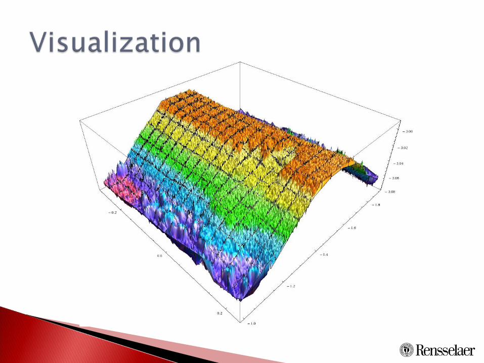
◦ Data Collection◦ Visualization
Findings Conclusions and Future Considerations Acknowledgement
Past failures have prompted the study of erosion on earthen embankments◦ Teton Dam (1976)◦ New Orleans’ Levees after Hurricane Katrina
(2005) Determine time required for erosion
processes to occur Understand rill and gully initiation and
propagation Visualize using software Create digital simulations Increase estimation capabilities

Levees are designed to protect areas adjacent to bodies of water from flooding
Poor design/construction can lead to disasters
Multiple failure mechanisms when subjected to water loading◦ Overtopping◦ Surface Erosion◦ Internal Erosion◦ Instabilities within embankment or foundation
soils
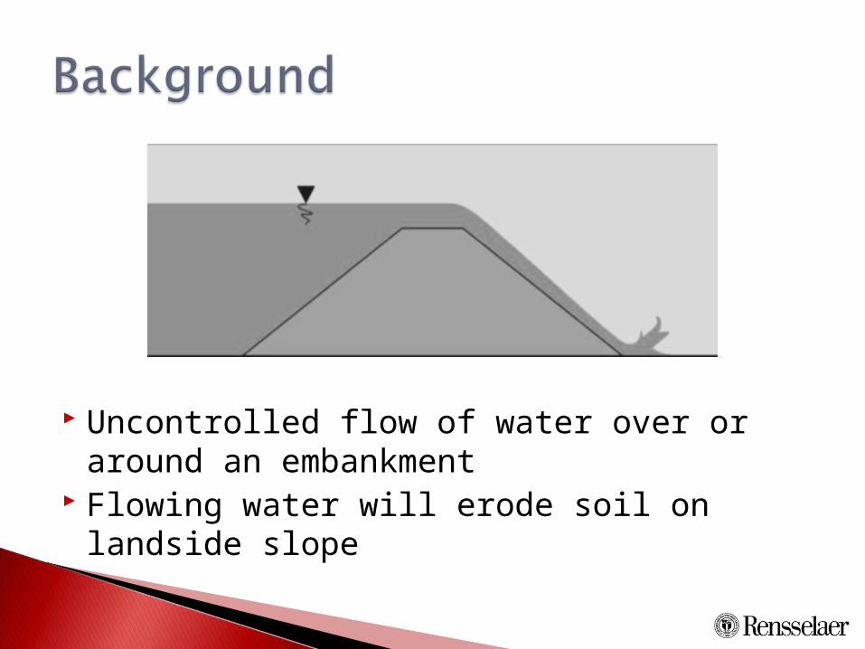
Uncontrolled flow of water over or around an embankment
Flowing water will erode soil on landside slope
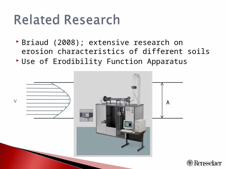
Briaud (2008); extensive research on erosion characteristics of different soils
Use of Erodibility Function Apparatus
Av
1 mm

Soil Erodibility◦ Relationship between water velocity and rate of erosion
experienced by soil Cohesive: Low Erodibility Granular: High Erodibility
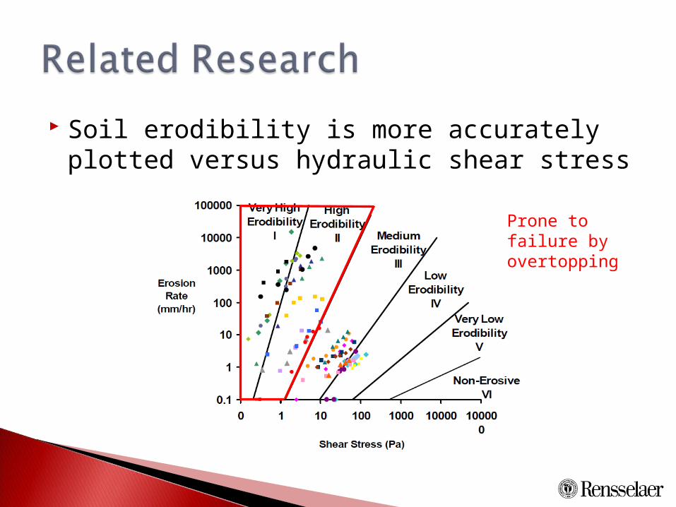
Soil erodibility is more accurately plotted versus hydraulic shear stress
Prone to failure by overtopping

Three departments are involved with the levee erosion research:◦ Civil & Environmental Engineering◦ Computer Science◦ Electrical, Computer and Systems Engineering
Each member has unique roles that partially overlap with roles of other members ◦ Produces new insights into previously studied
areas
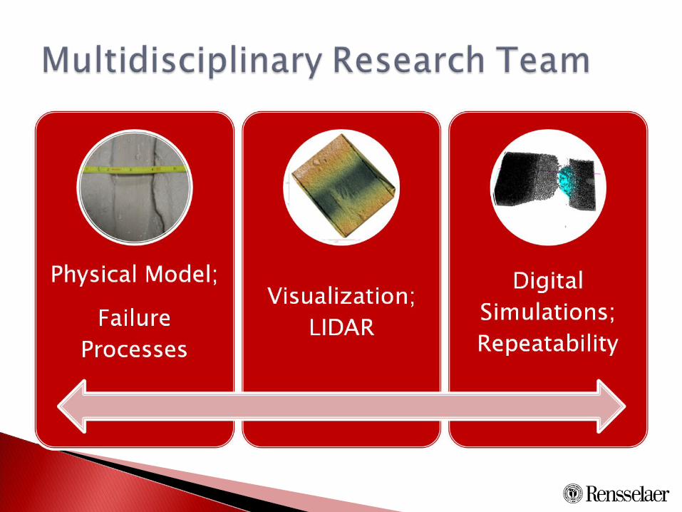

Physical model, post-laboratory erosion simulation
3D Laser Range Scanner
+

Purpose: validation On a small-scale levee Scans Videos

Model levees were constructed in an aluminum box (36” L x 24” W x 14” H)
Slopes were 1V:5H Different soils have been tested
◦ Medium-well graded sand◦ Nevada 90 sand◦ Nevada 90 sand – Kaolin clay mixture
Testing performed with and without low-permeability core
Water supply on waterside, drain on landside of model

Supply Drain

Laser beam emitted, scanner rotates and scans model at incremental rotations
Collects “slices” of elevation data from model
Data collected as a “point cloud”
Data is then aligned to an X-Y plane
A grid where each cell contains an array of soil layers with heights and depths results
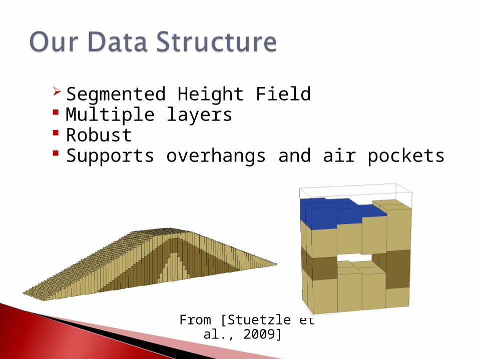
Segmented Height Field Multiple layers Robust Supports overhangs and air pockets
From [Stuetzle et al., 2009]

Data from scanner is loaded into data structure
Developed the Segmented Height Field data structure
Calculation of eroded volumes, channel widths, channel depths, etc.

Terrain represented by height fieldsSoil and water motion calculated by
terrain gradient
First Erosion Simulation Technique
From [Musgrave et al., 1989]
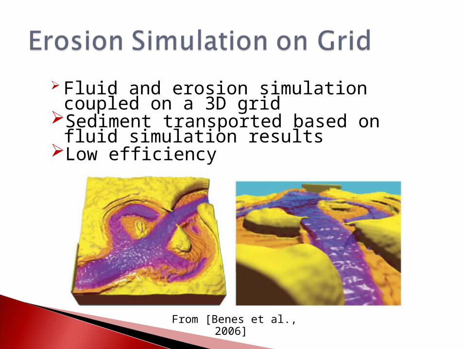
Fluid and erosion simulation coupled on a 3D grid
Sediment transported based on fluid simulation results
Low efficiency
From [Benes et al., 2006]

Marker-And-Cell (MAC) method
Navier-Stokes equations on a grid
Each cell with physical fields
Massless marker particles
From Foster and Metaxas, 1996

State of the system represented by particles
Based on interpolation theory Handles objects with large deformation or
mixed by different materials Save memory on void regions SPH particles Carriers of physical information Trackers of fluid surface

Terrain modeled as height field Fluid simulated by SPH Terrain surface is modeled as a
triangular mesh
From [Kristof et al, 2009]

From [Kristof et al., 2009]
Erosion rate ε is calculated by ε= Kε(τ- τc), where is Kε is erosion strength, τ is shear stress and τc is critical shear stress.
Two-step terrain modification:1. Erosion and deposition mass on each boundary
particle is calculated2. The height change of a triangle is calculated by the
total mass change of all particles in its area

Kernel approximation:
f is a field function defined in Ω, x is a point in Ω, W is a kernel function and h is the smoothing length.
Particle Approximation:
where x is the position of a point, Xj(j=1,2…,n) are positions of the particles neighboring X, mj is the mass and ρj is the density.
( ) ( ') ( ', ) 'f x f x W x x h dx
1
( ) ( ) ( , )N
jj j
j j
mf x f x W x x h
From [Muller et al., 2003]
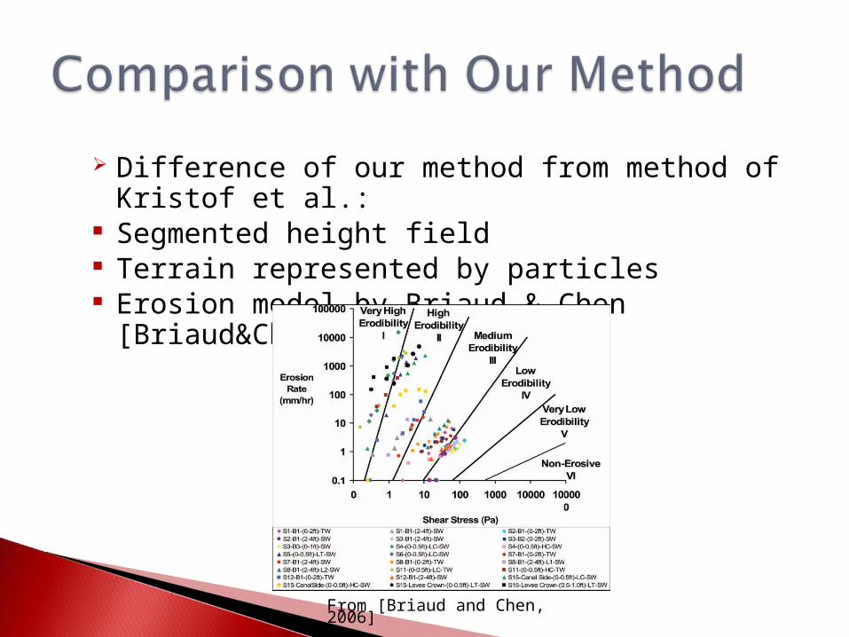
Difference of our method from method of Kristof et al.:
Segmented height field Terrain represented by particles Erosion model by Briaud & Chen [Briaud&Chen,
2006]
From [Briaud and Chen, 2006]

Spatial resolution: Soil particle spacing: 0.003m (2,500,000
particles)Water particle spacing: 0.004m (450,000
particles) Smoothing length: 0.008m Time step size: 0.001 seconds Time of running a 10-minute simulation: more
than a week (depending on the machine)

Computer simulation Pros: Various scales Whole process Details of gully Difficulty: Accuracy Efficiency

2 mins 5 mins 10 mins
Little Erosion
Much Erosion
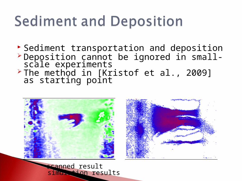
Sediment transportation and deposition Deposition cannot be ignored in small-
scale experiments The method in [Kristof et al., 2009] as
starting point
scanned result simulation results

Comparison and Validation

Models using a core did not fully breach unless a very low Q was used◦ Flow rate impacts rill characteristics
Sand models eroded grain-by-grain Sand-clay models eroded in larger clumped
masses Models with a core saturated more slowly,
eroded more slowly Clay content effects erosion and breach
failure times
Continued sand-clay mixture testing Centrifuge testing Flume testing Different soils Reinforcement/armoring Changes in levee geometry Digital simulation

Reverse engineering Helpful for people to look at the erosion
process Not possible to record the process Our goal is to reversely simulate the erosion
process based on the shape of the eroded levee

This research is supported by the National Science Foundation grant CMMI-0835762

Questions?