WAIT: Workshop on the Advances in Information Technology, Budapest, 2015

Simulating snow with the material point method

Tamás Umenhoffer1

1 Department of Control Engineering and Informatics, Budapest University of Technology and Economics, Budapest, Hungary

Abstract

In this paper we describe a full pipeline for physically accurate dense snow simulation. Our system uses the mate-rial point method to simulate packs of snow as an elasto-plastic material. We focused on efficient implementationthat fits into an animation and rendering pipeline typically used in motion picture production. We describe thematerial point method in details and list the tools that can help us to integrate the simulation into a renderingpipeline.

Categories and Subject Descriptors (according to ACM CCS): I.3.7 [Computer Graphics]: Animation

1. Introduction

Reproducing snow dynamics is a complex problem, as snowhas various behaviour depending on whether we are talkingabout falling snowball, packing snow, footsteps in snow, orpowder snow. We can notice that snow sometimes behavesas a fluid, but sometimes behave as an elastic solid. Unfortu-nately snow changes this behaviour continuously, so we cannot choose only a fluid or a solid simulator for a given effect.

Figure 1: Frames of an animation of a dropped snowballsimulated with the material point method.

Snow can be thought as a granular material, whose be-haviour is mostly directed by inter-granular friction. Somegraphics papers use simplified particle or rigid body systems5, 2. However it is hard to keep efficiency when increasing

the detail, thus increasing the number of grains. This lead re-searchers to apply continuum models 11, 3, 6, 1. One effectivemethod is the fluid implicit particles (FLIP) 11, which waseven used for human hair collision modelling4. FLIP is basi-cally a fluid simulation method dealing with incompressiblefluids. Fluid based methods model granular friction with vis-cosity. For some materials, and snow as well, compressibil-ity should be modelled. The material point method (MPM)9,was designed to extend FLIP to solid mechanics problemsthat require compressibility.

During the creation of the Disney movie titled Frozen, anMPM based method was introduced to simulate snow dy-namics for computer animation8. This work inspired us torecreate the technique and integrate it to our preferred ren-dering pipeline. We did not change the original algorithm,but reimplement it and developed the components that couldprovide the necessary input and output to and from the an-imation software, the simulation software and the renderer.We used Autodesk Maya as the animation package as it isthe most commonly used animation software in the movieindustry.

The MPM simulator tracks material properties at parti-cles, but uses an Eulerian background grid for computation,so we have to options to render out the simulation: using avolume renderer, or using a particle renderer. In contrast tothe original paper we used a particle renderer, as increas-ing quality is more effective with increasing particle countthan with increasing grid resolution. Increased 3D grid reso-

Umenhoffer / MPM Snow

Figure 2: Overview of our simulation pipeline.

lutions have too high memory and rendering computationalpower needs. Maya also can not handle high particle countseffectively, but a renderer plugin exists, that is developed es-pecially for this purpose. The Krakatoa renderer can handlemillions of particles, can be used inside Maya (which is im-portant for an instant visual feedback in Maya’s 3D view),or as an external renderer.

This paper continues with the overview of our system, de-scribing all the tools that are needed for a complete snowsimulation and rendering. Then the main steps of the mate-rial point method are presented to demonstrate the operationof our simulator application. Finally our experiences are dis-cussed.

2. System Overview

As we mentioned before our framework is based on Mayaand the Krakatoa particle renderer. Figure 2 shows anoverview of our simulation and rendering pipeline. For acomplete simulation, taking into account the geometry of thevirtual scene, the following problems should be solved.

First the initial snow particle positions should be given.For simple tests these positions can be filled procedurally,but for real scenes they are given by the artist. The easiestway is to model the volume of the snow and fill this volumewith particles. The Krakatoa plugin for Maya has a featureto fill a closed polygonal geometry with particles using auser defined particle density. These particles can be exportedinto Krakatoa’s particle file format and read by our simulatorapplication.

The second task is to export the scene geometry with ani-mations. This can be rather complicated as there are numer-ous different tools for animation in Maya. We can not pre-pare for all of them. However for such situations where onlythe final geometry is important and the concrete animationtools are not, we can cache the geometry in each frame andread it in the simulator. The computer animation communityalready created such a caching format and an open sourcelibrary for reading and writing. It is called Alembic, and thisformat is becoming a standard in animation industry.

Our simulator performs collision detection not on a tri-angular mesh but on a volume grid, so we have to voxelize

the exported geometry in each frame, and the simulator willread these voxel files instead of the geometry cache files.The problem with this voxelization is that we not only needto tell if a voxel is in the interior of a scene object, but wealso need to tell its normal vector and velocity. If we havea binary volume storing empty and filled voxels the normalscan be calculated relatively easily with central differences orhigher order gradient methods 7.

Calculating voxel velocities is not straightforward. 3D op-tical flow could not be used efficiently here as the voxelizedframes are binary, so most of the voxels will show no move-ment, and the rest will likely have aperture problem. How-ever during reading the geometry cache and assuming thatthe topology does not change (which is true for most of thecases), we can pair the vertices of two adjacent frames andcalculate their velocities with a simple subtraction. For eachinner voxel we find the nearest triangle, calculate the pro-jected barycentric coordinates of the voxel center and inter-polate a the velocity from the vertex velocities.

Fortunately an open source library exists for voxelizinggeometries and storing this sparse volumetric data in a hi-erarchical data structure. This library is called OpenVDB.OpenVDB also stores the nearest triangle index in eachvoxel, so we only have to implement the barycentric coor-dinate calculation and interpolation, and of course the nor-mal vector calculation. Normals can also be calculated withinterpolation, however if the geometry is complex comparedto the grid resolution, significant noise can appear. Our nor-mal calculation method is similar as in Thürmer et. all 10.For each voxel we define its 26 neighbouring directions (dk)and define the normal vector as:

N = ∑k

σkdk

where σk is minus one if the neighbouring voxel is aninner voxel and zero otherwise. We separated the voxelizerfrom the simulator, thus the voxelizer stores the voxel gridsin each frame in OpenVDB format, and the simulator takesthese files as input.

The simulator calculates updated particle positions ineach frame and stores these as Krakatoa particle files. Thesefile sequences are loaded back into Maya as a particle ani-mation and rendered with the Krakatoa renderer.

Umenhoffer / MPM Snow

Figure 3: Overview of the material point method (figure from 8).

3. MPM method

This section briefly describes the steps of the material pointmethod used in our simulation. For a detailed descriptionplease refer to 8. Figure 3 shows the main components of thesimulation. The algorithm can be described briefly as fol-lows. We track the material properties at particle positions.However some quantities are easier to compute on a grid, soour first step is to rasterize the particles onto a 3D grid. Nextcompute forces based on deformation gradients at each gridvoxel, and update grid velocities. Using these velocities weperform collision detection on the grid. The final velocitiesare transferred back to the particles. Then calculate a newdeformation gradient for each particle using refreshed voxelvelocities. Table 1 list the notations of parameters used in ourexpressions and gives their typical values where available.This table also serves as a useful guide for implementingthe MPM method, as all important particle and grid proper-ties are listed. The next subsections describe the steps of theMPM simulation in more detail.

3.1. Rasterize particles

Each simulation frame starts with transferring particle veloc-ities and mass to grid voxels, and ends with transferring up-dated velocities back to the particles. The grid can be thrownaway at the end of each simulation step, so it can be rede-fined at the beginning of the simulation step, and can be fitto the actual particle positions. However for implementationreasons we used fixed grid position and resolution.

The connection between particles and the grid is achievedwith an interpolation function. We used the same functionas in 8, which use dyadic products of one-dimensional cubicB-splines. When transferring particle data, we compute theweights in a 5x5x5 voxel neighbourhood of each particle,and add the scaled particle quantity to the voxel value:

mni = ∑

pmpwn

ip

Name Notation Typical values

Global parameters

Young modulus E0 1.4×105

Poisson ratio ν 0.2Critical compression θc 2.5×10−2

Critical stretch θs 7.5×10−3Hardening coefficient ξ 10

Particle data

Initial density ρp0 400Initial volume Vp0

Elastic force FEp

Plastic force FPp

Rotational force REp

Elastic determinant JEp

Cell data

Mass miVelocity vi

Force fiCollider flag coi

Collider velocity vcoi

Collider normal ncoi

Table 1: Notation of parameters used in our simulationframework. Default values are also listed where possible.

vni = ∑

pvn

pmpwnip/mn

i

When transferring voxel data back to particles, we againsample the 5x5x5 voxel neighbourhood of each particle, andsum their weighted average:

vnp = ∑

ivn

i wnip

Umenhoffer / MPM Snow

Because of the additivity, if we are interested in the deriva-tive of one quantity we can simply transfer with the deriva-tive of the weight function.

3.2. Particle volume and density

As an initial step particle density and volume should also becalculated. After rasterizing particle mass, density is givenwith the following expression:

ρ0p = ∑

im0

i w0ip/h3

Particle volume can be calculated from particle mass anddensity:

V 0p = mp/ρ0

p

These values are initial values, they are not going tochange during simulation.

3.3. Compute forces

Calculating stress-based forces needs derivatives, which areeasier to evaluate on the grid rather on the particles. Stress-based forces are defined by the deformation gradient, the fi-nal expression of these forces is:

fi(x) =−∑p

V 0p · (2µTco−rot +λTcontour) · (Fn

Ep)T ·∇wn

ip,

Tco−rot = FnEp

−RnEp,Tcontour = (Jn

Ep−1)Jn

EpFn

Ep

−T ,

where µ = µ(FP) = µ0 · eξ(1−JPp ),

and λ = λ(FP) = λ0eξ(1−JPp )

Here Pp and Ep are the plastic and elastic deformationsof a particle, JPp and JEp are their determinants. λ and µ arethe Lamè coefficients and can be computed from the Poissonratio and Young modulus in an initial step:

λ = E0(1+γ)(1−2γ) and µ = E0

2(1+γ)

3.4. Update velocities

If the stress based forces are calculated, voxel velocities canbe updated:

v∗i = vni +△t/mi · f n

i

Here we can also add the effect of any additional externalforces like gravity.

3.5. Grid based collision

Collision handling is performed on the voxelized scene ge-ometry after adding forces. An inelastic sliding collision isused. If the voxel is a collider cell and its velocity is notzero, the relative velocity is calculated: vreli = vi − vcoi . Ifthe relative velocity has opposing direction with the collidernormal (thus the particle and the collider are not separating),

only the tangential component of the velocity vector is kept.After this collision handling step we can finalize our voxelvelocities vn+1

i .

Here we should note that 8 used a semi-implicit inte-gration scheme here, which had much better accuracy, sosmaller time steps could be used. Due to its high implemen-tation complexity and additional memory needs we did notimplement it. This results about five times longer simulationtimes in our system.

3.6. Update deform gradient

From the updated velocities the deformation gradient of eachparticle should be calculated. This gradient is divided into aplastic and an elastic part FEp and FPp . First we assume thatall changes are attributed to the elastic part:

F̂n+1EP

= (I +△t∇vn+1p )Fn

EP,

F̂n+1Pp

= FnPp

,

where ∇vn+1p = ∑

ivn+1

i (∇wnip)

T .

The next step is to extract the stretching part of this gra-dient, and identify the amount of deformation the materialcould not hold, thus it breaks. This is done with a singularvalue decomposition and clamping the singular values:

SV D(Fn+1Ep

) =UpΣ̂pV Tp ,

Σp = clamp(Σ̂p, [1−θc,1+θc])

From the clamped singular values we can recalculate theelastic and plastic deformation gradients:

Fn+1Ep

=UpΣpV Tp ,

Fn+1Pp

= Fn+1Ep

−1F̂n+1

EpF̂n+1

Pp=VpΣ−1

p UTp F̂n+1

EpFn

Pp

These gradients will be used in the next simulation step tocalculate stress-based forces.

3.7. Update particle velocities

Now that each voxel stores an updated velocity, these ve-locities should be written back to the particles. We use thesame interpolation functions as for voxelizing particle data.Basically two methods can be used to update velocities: in-terpolate new velocities or interpolate the velocity change.The former is the classical particle in cell (PIC) method, thelater is used in the fluid implicit particles (FLIP) method. Forbest results these two solutions should be mixed:

V n+1p = (1−α)(∑

ivn+1

i wnip)+α(vn

p +∑i(vn+1

i − vni )w

nip)

We used α = 0.9.

Umenhoffer / MPM Snow

3.8. Particle based collision

An additional collision handling step is needed as interpola-tion can bring back collision errors. We do the same calcula-tions as in grid collision handling, but use particle velocitiesinstead of voxel velocities, and address the grid cell the par-ticle is in for collider information.

3.9. Update particle positions

Particles can be advected using their new velocities:

xn+1p = xn

p +△tvn+1p

4. Conclusions

We introduced a reimplementation of the material pointmethod for snow simulation. We also showed what tools canbe used to efficiently integrate the simulation into an anima-tion pipeline. The final framework is effective and easy touse. It supports any kind of animation on the scene objects.

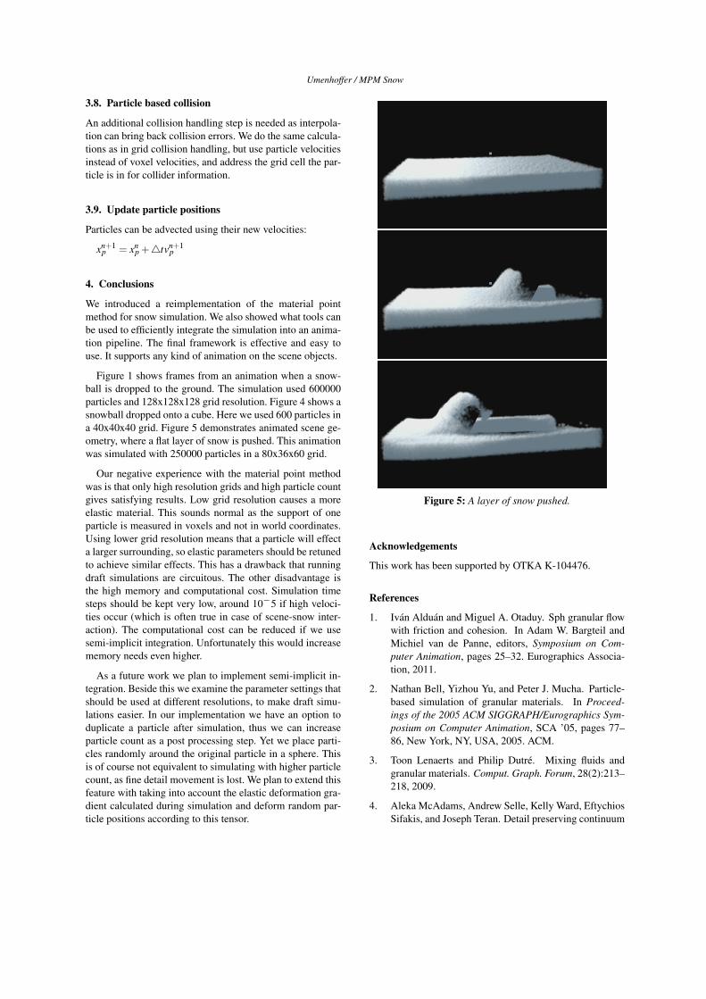
Figure 1 shows frames from an animation when a snow-ball is dropped to the ground. The simulation used 600000particles and 128x128x128 grid resolution. Figure 4 shows asnowball dropped onto a cube. Here we used 600 particles ina 40x40x40 grid. Figure 5 demonstrates animated scene ge-ometry, where a flat layer of snow is pushed. This animationwas simulated with 250000 particles in a 80x36x60 grid.

Our negative experience with the material point methodwas is that only high resolution grids and high particle countgives satisfying results. Low grid resolution causes a moreelastic material. This sounds normal as the support of oneparticle is measured in voxels and not in world coordinates.Using lower grid resolution means that a particle will effecta larger surrounding, so elastic parameters should be retunedto achieve similar effects. This has a drawback that runningdraft simulations are circuitous. The other disadvantage isthe high memory and computational cost. Simulation timesteps should be kept very low, around 10−5 if high veloci-ties occur (which is often true in case of scene-snow inter-action). The computational cost can be reduced if we usesemi-implicit integration. Unfortunately this would increasememory needs even higher.

As a future work we plan to implement semi-implicit in-tegration. Beside this we examine the parameter settings thatshould be used at different resolutions, to make draft simu-lations easier. In our implementation we have an option toduplicate a particle after simulation, thus we can increaseparticle count as a post processing step. Yet we place parti-cles randomly around the original particle in a sphere. Thisis of course not equivalent to simulating with higher particlecount, as fine detail movement is lost. We plan to extend thisfeature with taking into account the elastic deformation gra-dient calculated during simulation and deform random par-ticle positions according to this tensor.

Figure 5: A layer of snow pushed.

Acknowledgements

This work has been supported by OTKA K-104476.

References

1. Iván Alduán and Miguel A. Otaduy. Sph granular flowwith friction and cohesion. In Adam W. Bargteil andMichiel van de Panne, editors, Symposium on Com-puter Animation, pages 25–32. Eurographics Associa-tion, 2011.

2. Nathan Bell, Yizhou Yu, and Peter J. Mucha. Particle-based simulation of granular materials. In Proceed-ings of the 2005 ACM SIGGRAPH/Eurographics Sym-posium on Computer Animation, SCA ’05, pages 77–86, New York, NY, USA, 2005. ACM.

3. Toon Lenaerts and Philip Dutré. Mixing fluids andgranular materials. Comput. Graph. Forum, 28(2):213–218, 2009.

4. Aleka McAdams, Andrew Selle, Kelly Ward, EftychiosSifakis, and Joseph Teran. Detail preserving continuum

Umenhoffer / MPM Snow

Figure 4: A snowball dropped onto the edge of a cube.

simulation of straight hair. ACM Trans. Graph., 28(3),2009.

5. Victor J. Milenkovic. Position-based physics: Simulat-ing the motion of many highly interacting spheres andpolyhedra. In Proceedings of the 23rd Annual Con-ference on Computer Graphics and Interactive Tech-niques, SIGGRAPH ’96, pages 129–136, New York,NY, USA, 1996. ACM.

6. Rahul Narain, Abhinav Golas, and Ming C. Lin. Free-flowing granular materials with two-way solid cou-pling. ACM Trans. Graph., 29(6):173, 2010.

7. László Neumann, Balázs Csébfalvi, Andreas König,and Eduard Gröller. Gradient estimation in volume datausing 4d linear regression, 2000.

8. Alexey Stomakhin, Craig Schroeder, Lawrence Chai,Joseph Teran, and Andrew Selle. A material pointmethod for snow simulation. ACM Trans. Graph.,32(4):102:1–102:10, July 2013.

9. D. Sulsky, S.-J. Zhou, and H. L. Schreyer. Applicationof particle-in-cell method to solid mechanics. Comp.Phys. Comm., 87:236–252, 1995.

10. G. Thürmer and C. A. Wüthrich. Normal computationfor discrete surfaces in 3d space. Computer GraphicsForum (Proceedings of EUROGRAPHICS 97), pages15–26, 1997.

11. Yongning Zhu and Robert Bridson. Animating sand asa fluid. ACM Trans. Graph., 24(3):965–972, 2005.