Simulating soil freeze/thaw dynamics with an improved pan-Arctic water

balance model

M. A. Rawlins,1 D. J. Nicolsky,2 K. C. McDonald,3,4 and V. E. Romanovsky2

Received 30 October 2012; revised 2 July 2013; accepted 15 July 2013.

[1] The terrestrial Arctic water cycle is strongly influenced by the presence of perma-frost, which is at present degrading as a result of warming. In this study, we describeimprovements to the representation of processes in the pan-Arctic Water BalanceModel (PWBM) and evaluate simulated soil temperature at four sites in Alaska andactive-layer thickness (ALT) across the pan-Arctic drainage basin. Model improve-ments include new parameterizations for thermal and hydraulic properties of organicsoils; an updated snow model, which accounts for seasonal changes in density andthermal conductivity; and a new soil freezing and thawing model, which simulatesheat conduction with phase change. When compared against observations acrossAlaska within differing landscape vegetation conditions in close proximity to oneanother, PWBM simulations show no systematic soil temperature bias. Simulated tem-peratures agree well with observations in summer. In winter, results are mixed, withboth positive and negative biases noted at times. In two pan-Arctic simulations forcedwith atmospheric reanalysis, the model captures the mean in observed ALT, althoughpredictability as measured by correlation is limited. The geographic pattern in north-ern hemisphere permafrost area is well estimated. Simulated permafrost area differsfrom observed extent by 7 and 17% for the two model runs. Results of two simulationsfor the periods 1996–1999 and 2066–2069 for a single grid cell in central Alaska illus-trate the potential for a drying of soils in the presence of increases in ALT, annualtotal precipitation, and winter snowfall.

Citation: Rawlins, M. A., D. J. Nicolsky, K. C. McDonald, and V. E. Romanovsky (2013), Simulating soil freeze/thaw dynamics

with an improved pan-Arctic water balance model, J. Adv. Model. Earth Syst., 5, doi:10.1002/jame.20045.

1. Introduction

[2] Water is a dynamic element of the climate, biol-ogy, and biogeochemistry of the Arctic. Evidence hasmounted that the arctic system is now experiencing anunprecedented degree of environmental change duelargely to climatic warming [Serreze et al., 2000; Hinz-man, 2005; White et al., 2007]. Permafrost temperatureshave warmed [Christiansen et al., 2010; Romanovsky etal., 2010a, 2010b; Smith et al., 2010] and active-layerthicknesses have increased in many regions of theNorthern Hemisphere [Zhang et al., 2005; Wu and

Zhang, 2010]. There is evidence that the arctic fresh-water cycle is intensifying [Peterson et al., 2002, 2006;Rawlins et al., 2010]. Smith et al. [2007] documented anincrease in minimum daily flows across northern Russiaand speculated a connection to reduced soil freezing to-gether with an increase in precipitation. Permafrost isthe major control on hydrological dynamics at the localscale [Yoshikawa and Hinzman, 2003]. It is expected thatas permafrost continues to degrade the arctic terrestrialfreshwater system will transition from a surface water-dominated system to a groundwater-dominated system[Frey and McClelland, 2009]. Advances in understand-ing of these changes require the continued developmentof process-based models which accurately capture spa-tial and temporal dynamics and linkages between keyelements of the arctic freshwater system.

[3] The Pan-Arctic Water Balance Model (PWBM),advanced from a more generic Water Balance Modelfirst described by Vorosmarty et al. [1989], simulates allmajor elements of the terrestrial arctic water cycle. It isan implicit daily time step model and is forced at theatmosphere-land surface boundary with meteorologicaldata. In other words, the simulations are analogous to

1Department of Geosciences, University of Massachusetts,Amherst, Massachusetts, USA.

2Geophysical Institute, University of Alaska Fairbanks, Fair-banks, Alaska, USA.

3Department of Earth and Atmospheric Sciences, City College ofNew York, City University of New York, New York, USA.

4Jet Propulsion Laboratory, California Institute of Technology,Pasadena, California, USA.

©2013. American Geophysical Union. All Rights Reserved.1942-2466/13/10.1002/jame.20045

1

JOURNAL OF ADVANCES IN MODELING EARTH SYSTEMS, VOL. 5, 1–17, doi:10.1002/jame.20045, 2013

an offline simulation by an uncoupled LSM. It has beenused to investigate causes behind the record Eurasiandischarge in 2007 [Rawlins et al., 2009], to corroborateremote sensing estimates of surface water dynamics[Schroeder et al., 2010], and to quantify present andfuture water cycle changes in the area of Nome, Alaska[Clilverd et al., 2011]. In a comparison against observedriver discharge, PWBM-simulated SWE fields com-pared favorably [Rawlins et al., 2007]. The updated ver-sion of PWBM described here follows on improvementsto the Community Land Model (CLM) as outlined inNicolsky et al. [2007]. Structurally, the prior version ofPWBM differed from this new updated version in twokey ways: (i) it contained only two soil layers (rootingzone, deep soil zone) and (ii) active-layer evolution wasestimated using the Stefan solution of the heat-transferproblem. The Stefan solution requires estimation ofempirically derived landcover-specific parameters knowas ‘‘edaphic factors’’ to convert accumulated energy(e.g., thawing degree days) into a depth of thaw giventhe specific thermal properties of local vegetation andsoils.

[4] It has been demonstrated that numerical modelsimulations of soil freezing and thawing require atten-tion to several key processes operating across the land-scape [Nicolsky et al., 2007; Lawrence and Slater, 2008;Rinke et al., 2008; Schaefer et al., 2011]. For example,thermal and hydrological properties of organic andmineral soils differ considerably. Improvements in per-mafrost distribution, active-layer thickness, and deepground temperatures have been documented in theCLM4 [Lawrence et al., 2012]. Swenson et al. [2012]described modifications to CLM4 hydraulic permeabil-ity when soils are frozen which corrected a dry bias.Upgrades as well have been made to the SiBCASAmodel, including the addition of parameterizationswhich account for the effect of depth hoar and windcompaction on simulated snow density [Schaefer et al.,

2009]. Wisser et al. [2011] described model improve-ments which centered on the explicit representation ofpeatlands and their associated properties. Jiang et al.[2012] explored the effects of climate change and fire onsoil temperatures using a soil thermal model that cou-ples heat and water transport.

[5] The present paper centers on descriptions ofnew components and analysis of results from animproved version of Pan-Arctic Water BalanceModel (PWBM). Upgrades to the model enable morephysically based simulations of snow and soil dy-namics. Our primary domain is the pan-Arctic drain-age basin. Grid resolution is the 25 3 25 km2

version of the northern hemisphere Equal Area Scal-able Grid (EASE-Grid). Following a description ofthe model and data sources, our analysis begins withcomparisons between simulated and observed soiltemperatures for four sites in Alaska. We then evalu-ate results and explore model performance at thepan-Arctic scale. Lastly, we use projections for futureprecipitation and air temperature for a representativelocation in central Alaska to investigate potentialchanges in the soil regime and connections withexpected climatic changes.

2. Modification to the PWBM

2.1. Soil Model

[6] Figure 1 depicts a schematic representation of theupdated PWBM described in this paper. The updatedPWBM soil model discretizes a 60 meter soil columnwhich contains 23 layers, with layer thickness increasingwith depth. The model simulates snow/ground tempera-ture dynamics in a more physically based manner, usingthe 1-D heat equation with phase change

Figure 1. Schematic of PWBM soil profiles for winter (left), spring (center), and summer (right). Transitions backto frozen condition during autumn not shown. The model develops an active layer in spring which allows for watergains through infiltration and losses from runoff and evapotranspiration (ET). Water pools on the surface if infil-tration capacity is exceeded. Drainage between layers follows Darcy’s Law as solved through the Richard’s equa-tion. The model incorporates subgrid scale open water extents. Temporally varying change in water table height isalso simulated.

RAWLINS ET AL.: SOIL FREEZE/THAW MODELING

2

C@T

@t1Lf

@h@t

5@

@zk@T

@z

� �; z 2 zs; zb½ � ð1Þ

and diffusive and gravitational movement of water inthawed ground by solving Richard’s equation

@f@t

5@

@zk@w@z

11

� �� �; z 2 0; zb½ �: ð2Þ

[7] Here T 5 T(z, t) is the temperature, f5f z; tð Þ is thevolumetric water content, w5w z; tð Þ is the soil matrixpotential. The quantities C5C T ; zð Þ Jm23K21

� �and

k5k T ; zð Þ Wm21K21� �

represents the volumetric heatcapacity and thermal conductivity of soil, respectively;L Jm23� �

is the volumetric latent heat of fusion ofwater, and h5h T ; zð Þ is the so-called ‘‘unfrozen liquidpore water’’ fraction, and k 5 k(T, z) is the hydraulicconductivity. Details of the numerical solution of theheat equation can be found in Appendix A. The inter-ested reader may consult the CLM 4.0 technicaldescription for details of the numerical solution of theRichard’s equation. The equations are solved implicitlywith a daily time step. At the upper boundary conditionair temperature and precipitation are prescribed asdescribed below. We emphasize that equation (2) is ap-plicable only for the thawed ground material. In orderto extend to simulations of water motion in frozenground, some models (e.g., CLM 4.0 [Oleson et al.,2010]) propose that w5w T ; h; xð Þ if T<Tp, where Tp isthe so-called freezing-point temperature depression. Inthis work, we assume that the water migration in thefrozen ground is negligibly small. The latter can bemodeled by assuming that the coefficient of hydraulicconductivity k(T, z) 5 0, if T<Tp. Thus, when a layerof the ground material becomes frozen the total watercontent f in it stays constant until the moment when thelayer becomes thawed again. Note that for frozen soillayers the matric potential can be arbitrarily defined,since it does not enter into calculations, and the waterflux boundary condition is imposed at the bottom ofthe thawed region. Another distinction of the proposedmodel from the CLM is the way soil thermal propertiesare parameterized. Additional information is providedin Appendix A.

2.2. Snow Model

[8] Seasonal snow cover has a significant influence onthe ground thermal regime [Zhang, 2005]. For example,

snowcover provides an insulating layer and limits thedegree of soil cooling during cold winter months. Clas-sification maps derived from wind, precipitation, andair temperature data [Sturm et al., 1995] can be used toinfer snow thermal and physical properties for simula-tions with numerical models. Land surface models(LSMs) capable of simulating soil freeze/thaw dynamicshave recently begun to focus on the effects of snow onunderlying soil temperatures.

[9] Formulations in the PWBM for snow accumula-tion, sublimation, melt, and associated processes aredescribed in Rawlins et al. [2003]. The simulated snow-pack contains both a solid and a liquid portion, providinga total model estimate for snow water equivalent (SWE).New routines to account for seasonal changes in snowdensity follow on recent improvements to the CLMand to the Simple Biosphere/Carnegie-Ames-StanfordApproach (SiBCASA). The CLM version 4 includes asnow model which simulates processes such as accumula-tion, melt, compaction, snow aging [Lawrence et al.,2012]. The Simple Biosphere/Carnegie-Ames-StanfordApproach (SiBCASA) uses the snow classification systemof Sturm et al. [1995], and a snow model derived from theCLM. We take here a similar approach in modeling thetemporal evolution in snowpack density. Details of ournew snow density model are described in Appendix A.

2.3. Organic Content and Parameterizations

[10] In many parts of the Arctic where soil carbon ishigh, the first 40–50 cm of soil is nearly 100% organic,with a transition from organic to mineral soil and 100%mineral soil below. In the middle transition zone, ther-mal and hydraulic properties of mixed mineral and or-ganic soil material can be approximated as a weightedcombination of the mineral soil and organic soil proper-ties. As described in Rawlins et al. [2003], the previousversion of PWBM contained an upper organic layer anda lower mineral layer imposed in the two layer profile.

[11] In order to better account for the thermal andhydrologic properties of soils, we parameterized carbondensity in each soil layer. We take a similar but notidentical approach to the one described in Lawrence andSlater [2008]. The Global Soil Data Task (GSDT, 2000)data set contains soil-carbon density (C, kg m23) acrossthe depth interval of 0–1 m. To obtain C across thepan-Arctic basin, we averaged the five arc-secondGSDT data for each EASE-Grid cell. We applied thesoil profile for polar and boreal soils from Zinke et al.

Table 1. Soil Parameters Used in the PWBM Simulationsa

Soil Type k (W m21 K21) C (J m23 K21 3 106) Hsat ksat (m s21 3 1023) Wsat (mm) b

Sand km 5 3.6 Cm 5 3.0 0.25 0.023 247 3.4Loam km 5 3.0 Cm 5 3.0 0.35 0.042 2207 6.1Clay km 5 2.3 Cm 5 3.0 0.45 0.020 2390 12.1Sandy loam km 5 3.3 Cm 5 3.0 0.40 0.071 2132 4.5Clay loam km 5 2.6 Cm 5 3.0 0.39 0.028 2289 8.2Organic soil ko 5 1.5 C0 5 1.9 0.9 0.02 2120 2.7

aEach grid cell in the model is characterized by one of the five mineral soil types. Model parameters are defined through a weighted combina-tion of organic and mineral soil properties. See Rawlins et al. [2003] for more detail on the PWBM soil routine.

RAWLINS ET AL.: SOIL FREEZE/THAW MODELING

3

[1986] to obtain carbon storage over the top 11 modelsoil layers (1.4 m depth). Soil carbon or organic fractionfor each layer was then determined as

fsc;i5qsc;i=qsc;max ð3Þ

where fsc;i is the carbon fraction of each layer i, qsc;i isthe soil carbon density, and qsc;max is the maximum pos-sible value (peat density of 130 kg m23, Farouki [1981]).Soil properties for each layer are specified as a weightedcombination of organic and mineral soil properties

P5 12fð ÞPm1fPo ð4Þ

where f is the fraction of organic material in the soillayer, Pm is the value for mineral soil, Po is the valuefor organic soil, and P is the weighted average quantity.Thermal and hydrologic parameters as a function ofsoil class are listed in Table 1.

3. Data Sets

3.1. Forcing Data

[12] Many of the static input data fields (e.g., soilproperties, landcover type, and snow class) and meteor-

ological forcings used in the prior and present versionof the PWBM are available within the ArcticRIMS pro-ject archive (http://rims.unh.edu/). For the two pan-Arctic simulations, we draw daily 2 m air temperature,precipitation, and wind speed from two atmosphericreanalyses data sets. Atmospheric reanalyses are retro-spective forms of numerical weather prediction using afixed model and data assimilation system. The first(hereafter referred to as NNR) was derived from theNCEP/NCAR (National Centers for EnvironmentalPrediction/National Center for Atmospheric Research)effort [Kalnay et al., 1996] (in ArcticRIMS see: http://rims.unh.edu/data/read_me.cgi?category57&subject50and http://rims.unh.edu/data/read_me.cgi?category52&subject50). The second set of reanalysis data (here-after ERA-40) was drawn from the European Centerfor Medium Range Weather Forecasts (ECMWF)ERA-40 reanalysis [Uppala et al., 2005] (in ArcticRIMSsee: http://rims.unh.edu/data/read_me.cgi?category57&subject58 and http://rims.unh.edu/data/read_me.cgi?category52&subject55). No ERA-40 wind speed datais available in Arctic-RIMS and so NNR wind speedare used in their place for the simulations describedbelow.

[13] Across the terrestrial Arctic, total precipitationover cold season months can be used as a proxy for

Figure 2. Research sites used for model evaluations: Bonanza Creek (B); Coldfoot (C); Council (L); Dietrich (D). Bo-nanza Creek, Coldfoot, and Dietrich are in the Alaska Ecological Transect (ALECTRA) network. Filled circles markother ALECTRA sites. Landcover units within each respective site are listed in Table 2. Colors denote landcover classhttp://ecosystems.mbl.edu/tem/GIS/Veg/temveg.htm on the 25 3 25 km2 EASE-Grid used in the simulations.

RAWLINS ET AL.: SOIL FREEZE/THAW MODELING

4

snowfall. As a first step, we assessed biases in NNR andERA-40 total precipitation for November–March usingprecipitation data available from the University of Del-aware (UDel) [Matsuura and Willmott, 2009; Willmottand Matsuura, 2000]. The UDel data sets were devel-oped through interpolations of meteorological stationdata records. For this assessment, average November–March precipitation was taken over the period 1980–1999. Bias maps are shown in Figures 2a and 2b. Thedistribution of biases is largely positive across the pan-Arctic. Integrated area average biases (excluding Green-land) are 0.17 and 0.24 mm day21 for NNR and ERA-40, respectively. Across Alaska, biases are also mostlypositive. For the region west of 135�W, averagesare 0.21 mm day21 for NNR and 0.31 mm day21 forERA-40.

3.2. Ground-Based Validation Data

[14] Evaluations of model simulated soil tempera-tures are made using multiple within-site observationsfrom a subset of the Alaska Ecological Transect(ALECTRA) sites (Figure 3). We chose ALECTRAsites that have sufficient multiyear data over the period2000–2005. The evaluation sites are Bonanza Creek,Coldfoot, and Dietrich (Table 2). Missing data due tologger or sensor issues limit the number of sitesavailable for examination. The ALECTRA sites wereconceived and implemented to capture spatial hetero-geneity in soil and vegetation stem/branch temperatureconditions across the landscape that largely reflectmicroclimatic variability. Many of the ALECTRAsites are situated near research stations where meteoro-logical observations are available. The sites are distrib-uted along a north-south latitudinal transect extendingfrom Arctic coastal tundra through the boreal and intomaritime forest. Soil temperature and snow data forCouncil were drawn from records archived at the Uni-versity of Alaska Water and Environment ResearchCenter (http://ine.uaf.edu/werc/). For the simulationsat each of the four research sites (Table 2), we used theaverage 2 m air temperatures across available sites.Precipitation and wind speed were drawn from theNNR.

[15] Observations of ALT from the CircumpolarActive Layer Monitoring (CALM) data set [Brown etal., 2000] are used to evaluate PWBM simulated esti-mates. Field sampling in the CALM program typicallyinvolves measurements across a grid spanning 0.1 km2

or in some locations 1 km2 area. Each recorded ALTvalue represents maximum seasonal depth of thaw of

Table 2. Landscape Units Within the Respective Research Sitesa

Site Bonanza Creek Coldfoot Council Dietrich

Landscape unit South slope South slope Tundra South slopeLandscape unit Black spruce Black spruce Spruce White spruceLandscape unit White spruce Bog Shrub BogLandscape unit Willow swamp Woodland Creek

aData for Bonanza Creek, Coldfoot, and Dietrich are part of the Alaskan Ecological Transect (ALECTRA).

Figure 3. Bias in cold season (Nov–Apr) precipitationat each 25 3 25 km2 EASE-Grid across the pan-Arcticdrainage basin. Bias is defined as the difference betweenthe reanalysis and observed (UDel) precipitation totals.

RAWLINS ET AL.: SOIL FREEZE/THAW MODELING

5

the 121 samples. For our comparisons with PWBM-simulated values, we take the average of all nonmissingCALM ALTs over the period 1980–2011.

4. Results

4.1. Site Comparisons

[16] Figure 4 shows the simulated snowpack behaviorover several years for each of the four study sites. Ateach site, snow density increases through the cold sea-son, starting at around 100 kg m23. The profiles for Bo-nanza Creek and Coldfoot are similar, with snowdensities spanning a range between 100 and 250 kgm23. A larger range is evident for Dietrich and Council,where end-of-season snow density is over 300 kg m23.Comparing simulated snow depth with observationsreveals no consistent biases. In some years, there isgood agreement, in some years the model overestimatessnow depth, in other years it underestimates. This isworth noting given the positive bias (overestimate) incold season precipitation (Figure 3).

[17] The thermal conductivity of organic soils is low,ranging from 0.50 W m21 K21 at saturation to 0.06 W

m21 K21 under dry conditions [Farouki, 1981]. Figure 5shows model simulated thermal conductivity profilesfor May, June, September, and October at the foursites. For Bonanza Creek, Coldfoot, and Council thesimulated organic density as parameterized is nearly100% in upper 20 cm and transition to fully mineral soilat around 40 cm. Note the much thinner modeled or-ganic horizon for the Dietrich site. Simulated thermalconductivity there increases sharply down to around 30cm depth where it approaches 2.4 W m21 K21. ForDietrich, the reduced thermal conductivity in the soillayer centered at 0.55 m is largely attributable to lesserwater content. This soil layer is the lowest that thawsover the spin-up period during which time it loosessome water. During the simulation period, permafrostagain develops at this layer, however, the water contentand thermal conductivity then is lower. At each site,conductivities tend to be higher in spring versusautumn. This result reflects higher soil moistureamounts, and thus thermal conductivity, followingspring snowmelt.

[18] Soil temperatures are influenced by a number ofclimate and landscape factors [Callaghan et al., 2011].

Figure 4. Simulated snowfall (vertical bars, mm day21), snow water equivalent (mm), snow depth (cm), and snowdensity (kg m21) for the grid cells encompassing Bonanza Creek, Coldfoot, Council, and Dietrich sites. Availableobserved snow depths (red dots) shown for the first three sites.

RAWLINS ET AL.: SOIL FREEZE/THAW MODELING

6

The seasonal cycle in air temperature and seasonalaccumulation and melt of snowpack are perhaps thetwo most important processes that influence annualvariations in soil temperatures. Examining simulatedsoil temperatures against observed data providesinsights into model efficacy. Figures 6a and 6b showsimulated and observed daily soil temperatures at 25 cmdepth for Bonanza Creek and Coldfoot. Colored tracesrepresent temperatures from measurements in eachlandscape units within the research sites. For BonanzaCreek, model simulated summer temperatures are wellcaptured, falling between the warm south facing slopeand the cooler spruce sites. Model temperatures duringwinter are clearly too warm. At Coldfoot, summer tem-peratures again are well simulated. In contrast with Bo-nanza Creek, 25 cm temperatures during the first 5months of the year fall in the middle of the range ofobservations.

[19] Figure 7 depicts monthly average soil tempera-ture at both 25 and 50 cm depth for Bonanza Creek,Coldfoot, Council, and Dietrich. For Bonanza Creek,simulated temperatures in summer fall well within therange of the measured data from the three landscapeunits (Table 2). In winter, the model is warmer thanobservations, with simulated temperatures at 25 and 50

cm remaining near freezing through the winter. Modelsimulated snow depth compares well with observationsover the winters of 2000–2001 and 2001–2002 (Figure4). The warm soil temperature bias in winter 2002–2003is consistent with an overestimation in simulated snowdepths. Over the period 1980–2008, precipitation aver-ages 374 mm yr21 in the daily NNR data versus 286mm yr21 for National Weather Service observationsfrom Fairbanks International airport over the climatenormal period 1971–2000.

[20] For Coldfoot, model simulated soil temperaturesat 25 cm depth fall well within the measured rangeacross the landscape units during most months (Figure7). Simulated snow depths are lower than the observedvalues in two of the three years shown. The exception iswinter 2002–2003 when the model overestimates tem-peratures. Simulated temperatures at 50 cm depthremain near 0�C through summer, whereas the observa-tions are 1–4�C warmer.

[21] At Council, simulated temperatures are colderthan the observations by some 5�C during the coldestmonths (Figure 7). Simulated midwinter snow depths in2000–2001 were approximately half (40 versus 80 cm) ofthe observed values. This bias could explain some of thediscrepancy in simulated soil temperatures. With no

Figure 5. Simulated soil thermal conductivity (W m21 K21) with depth for the grid cell encompassing BonanzaCreek, Coldfoot, Council, and Dietrich sites for months May (black), June (red), September (green), and October(blue) in 2000 (2001 for Bonanza Creek). Gray shading indicates percent of organic carbon density in each soillayer.

RAWLINS ET AL.: SOIL FREEZE/THAW MODELING

7

south facing slope (Table 2), observed temperatures atCouncil are notably cooler than those at BonanzaCreek and Coldfoot sites. Both the annual temperaturecycle and the range in temperatures across the fourlandscape units at Council are small. Good agreementwith the observations occurs in summer each year,where the model and observations at 25 and 50 cm arein the range 0–5�C. The small variations around 0�C inthe winter 2000–2001 observations at Council may be aresult of a deep snowpack and/or a reflection of a thickorganic layer, both of which would tend to limit theinfluence of the overlying cold winter air.

[22] For Dietrich, simulated temperatures fall withinthe observed range during most months, excludingspring of 2004 and 2005 when simulated temperaturesare approximately 1–2�C colder than the observations(Figure 7). No observed snow depth data are availablefor Dietrich. Like with Bonanza Creek, Coldfoot, andCouncil sites, simulated temperatures in summer agreewell with observations. When compared with BonanzaCreek, the larger degree of cooling in the Dietrich simu-lation is largely a reflection of the thinner organic layerand, in turn, higher thermal conductivities (Figure 5).

[23] We performed a series of sensitivity experimentsto help elucidate potential sources of bias in simulatedsoil temperatures at depth during both the cold and

warm season. In particular, we examined the simulatedsoil temperatures at 25 cm at Bonanza Creek and Coun-cil sites. For Bonanza Creek, reducing snowfall over thecold season by 50% cools temperatures at the 25 cmdepth over the cold season (November–March, 2001–2000) by 2.3�C. These results suggest that any errors insnow depth can explain some but not all of the bias insimulated winter temperatures at depth. We then ana-lyzed the effect of errors in organic content (by carbondensity in the model) of soil layers by decreasing the or-ganic content by 50%. This change resulted in a coolingof temperatures by approximately 1�C. In view of theseresults, we speculate that a combination of errors insnow depth and organic layer thickness (carbon den-sity) could well explain most of the bias in simulatedsoil temperatures at depth. For Council, doubling ofcold season snowfall warms soil temperatures at 25 cm(1999–2000) by 3.6�C. This result suggests that errors inthe approximation of snow depth can explain most butnot all of the bias in the simulation results shown inFigure 7.

[24] We also performed a pair of experiments to bet-ter understand model sensitivity during the warm sea-son. For these simulations we simultaneously perturbedsoil layer carbon density and air temperature andfocused on Bonanza Creek sites. First, in order tomimic typical conditions across the south-facing slope,we approximated an organic layer thickness of 20 cmand as described above reparameterized the resultantcarbon density of each layer. At the same time, wescaled the input 2 m air temperatures upward by 2�C.In the second sensitivity experiment, we approximatecondition in either the white spruce or black sprucestand by parameterizing a 60 cm organic layer and re-sultant carbon densities at depth, along with 2�C coolertemperatures. A difference of 4.2�C was found betweenthe two simulations. Our results here demonstrate thatthe numerical soil freezing and thawing scheme, param-eterizations and input data for organic content, andinput air temperature forcings are able to capture muchof the variations in observed summer soil temperaturesacross the Bonanza Creek sites.

4.2. Simulated Active Layer Thickness and PermafrostExtent Across the Pan-Arctic

[25] To further evaluate model performance, we ranadditional simulations across the entire pan-Arcticdrainage basin. Model spin-up was performed through50 iterations over the year 1980, the first year of thetransient simulation. We use the daily precipitation, airtemperature, and wind data derived from the reanalysisproducts as described in section 3.1. A grid cell is la-beled as containing permafrost if at least one layerwithin the upper 15 soil layers (3.25 m depth) remainsfrozen throughout the year. Simulated ALT is esti-mated as the depth where soil temperature crosses the0�C threshold. In these evaluations, observed CALMALT represents all available nonmissing values for agiven site over the period 1980–2011.

[26] Figure 8 shows comparisons between simulatedand observed ALT over the period 1980–1999 from the

Figure 6. Daily soil temperatures at 25 cm depth simu-lated by the PWBM and from observations at (a) Bo-nanza Creek and (b) Coldfoot. A 7 day running mean isapplied to each time series. Available landscape sites foreach location are listed in Table 2.

RAWLINS ET AL.: SOIL FREEZE/THAW MODELING

8

prior (a,b) and updated (c,d) versions of PWBM. Simu-lated mean ALT is taken as the 30 year average for thegrid cell encompassing each respective CALM location.Mean biases (simulated minus observed ALT) from theprior version are 236 cm and 227 cm for the NNR andERA-40 simulations, respectively. With the updatedversion, biases are 24.0 cm and 5.9 cm for NNR andERA-40, respectively. A systematic underestimation ofALT is evident in simulations with the prior version. Itshould be noted that a scale mismatch exists in anycomparison involving grid-to-point observations. Whilethe updated model simulates well the mean among theobserved ALTs, it struggles with predictability. Thisshortcoming is not uncommon among numerical mod-els which simulate active layer dynamics [Su et al., 2005;Lawrence et al., 2012]. In a study of ALT estimatesacross northern Alaska produced by three differentmodels, Shiklomanov et al. [2007], found that large dif-ferences in ALT were attributable to the differentapproaches used for characterization of surface andsubsurface conditions. Measured ALT can vary sub-stantially over small distances. At any given location,ALT is influenced by several factors including thermalproperties of soil, snow characteristics, vegetation type,and soil moisture amount. It has been shown that varia-tions in ALT of up to 50% can occur over short distan-ces [Nelson et al., 1997].

[27] At the pan-Arctic scale, the PWBM captures wellthe north-south ALT gradient (Figure 9). Estimatesrange between 30 and 40 cm along the Arctic coast and

approach 1.5 m in parts of southern and western Siberiaand central Canada. The simulation with NNR forcings(Figure 9a) produces slightly greater ALTs compared tothe ERA-40 simulation (Figure 9b). Simulated perma-frost areal extent is 14.6 (14.4–14.8) 3 106 km2 and 13.3(13.0–13.6) 3 106 km2 from the NNR and ERA-40 sim-ulations, respectively. This compares with an observedarea of continuous plus discontinuous permafrost of12.5 3 (11.8–14.6) 106 km2 [Zhang et al., 2000]. Thus,our simulated areas are 7 and 17% above observedextent for the ERA-40 and NNR simulations, respec-tively. However, as Lawrence et al. [2012] noted, perma-frost area obtained from a coarse model is likely biasedhigh. If true, the 14.6 3 106 km2 (continuous plus dis-continuous permafrost) extent estimated by Zhang et al.[2000] would represent a better goal for modelsimulations.

[28] Figure 10 shows the results of a comparisonbetween simulated runoff in the present study (labeledPWBM2013) and those described in Rawlins et al. [2003](PWBM2003). Marked differences are evident. For theYenisei, Lena, and Yukon basins, annual runoff inthe present simulation is closer to observed values fromthe R-ArcticNet v4.0 archive (http://www.r-arcticnet.sr.unh.edu/v4.0/) [Lammers et al., 2001]. For the Oband Nelson basins, observed runoff is relatively low andsimulated runoff is clearly overestimated. Annualobserved runoff averaged over the pan-Arctic basin(1979–2001) is approximately 230 mm yr21 [Rawlinset al., 2010]. Comparing this recent estimate to the 180

Figure 7. Range in monthly soil temperatures at 25 (blue) and 50 cm (red) depth from observations (vertical lines)and model value at each of those depths (circles) across the available landscape units at Bonanza Creek, Coldfoot,Council, and Dietrich. For each month, the first bar/circle represents values for 25 cm and second for 50 cm. Avail-able landscape sites for each location are listed in Table 2.

RAWLINS ET AL.: SOIL FREEZE/THAW MODELING

9

mm yr21 (1980–2001) from Rawlins et al. [2003] gives abias (predicted minus observed) of approximately222%. Using the same NNR data as Rawlins et al.[2003] in the updated PWBM gives an annual runoff of250 mm yr21, a bias of 9%. We note that the observedrunoff/precipitation (R/P) ratio for the Nelson basins islow relative to other high latitude river basins.

[29] Figure 11 illustrates the differences in soil mois-ture distribution with depth between simulations withthe updated and prior model versions. It shows soilmoisture variations for the grid cell encompassing theBonanza Creek site from simulations forced with themeasured (site) daily air temperatures along with NNRprecipitation and wind data. The soil profile in the newversion exhibits expected patterns, with nearly saturatedmineral soils above the permafrost (Figure 11a). Upperorganic rich layers become wet following snowmelt andare considerably drier than the underlying mineral soils

in summer. ALT averages 68 cm, close to the meanobserved value of 55 cm from the CALM data set. Inthe prior version of the model (Figure 11b), the ALTreaches approximately 30 cm each year. Soil moisture islower as well. In the prior version, soil ice thaw was cal-culated based on the fraction of the layer which thawson a given day. This results in relatively higher soil iceand, hence, lower soil water amounts through summer.

4.3. Potential Future Changes in Near SurfaceConditions

[30] Lastly, we explored potential future changes insoil thermal and moisture regimes using data from theNorth American Regional Climate Change AssessmentProgram (NARCCAP, https://www.narccap.ucar.edu/).The NARCCAP [Mearns et al., 2007] is archiving out-puts from a set of regional climate model (RCM) simu-lations over a domain spanning North America. The

Figure 8. Scatter plot of CALM ALT and simulated ALT from the prior (PWBM2003)(a,b) and updated versionof the PWBM (PWBM2013)(c,d). Observed ALT is the average for available years for each site. Mean bias is 24.0and 5.9 cm for the NNR and ERA-40 PWBM2013 simulations, respectively. Mean bias is 236.5 and 227.0 for theNNR and ERA-40 PWBM2003 simulations, respectively. CALM sites across the Tibetan Plateau were excludedfrom the evaluation.

RAWLINS ET AL.: SOIL FREEZE/THAW MODELING

10

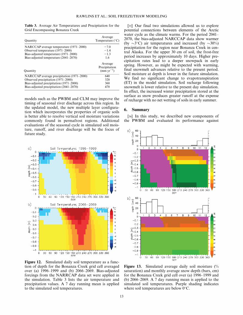
NARCCAP includes six RCMs, each forced withboundary conditions from two atmosphere-ocean gen-eral circulation models (GCMs). For each model pair-ing, air temperature and precipitation are available for

two 30 year periods: 1971–2000 and 2041–2070 (here-after present and future, respectively). From the nativeRCM grids, we selected the cell which encompasses theBonanza Creek area and averaged daily air temperatureand precipitation across the available GCM-RCM pair-ings. Wind speed was taken as the daily climatologyfrom the NRR data. Model spin-up for each 30 yearsimulation was performed by iterating over the firstyear of the present and future periods (1971 and 2041,respectively). For the grid chosen, a moderate cold andwet bias is present. To ameliorate the influence this biaswould place on results we scaled each daily time seriesusing monthly observations for Fairbanks Internationalairport. Table 3 lists original and bias-adjusted values.Temperature change between the future and presentperiods is 2.9�C and precipitation change is just over30%. As described below, our analysis of potentialchanges in ALT, thawed season length, soil temperatureand moisture focuses on averages over the periods1996–1999 and 2066–2069.

[31] Figure 12a shows simulated soil temperature as afunction of depth for the period 1996–1999. Forcing themodel with the bias-adjusted NARRCAP data resultsin a seasonally frozen (nonpermafrost) soil column. Wenote that average grid cell temperature over the 1971–1999 period with this simulation is just over 1.5�Cwarmer than the NNR and ERA-40 data. The absenceof permafrost here is not entirely unexpected as the areaaround Bonanza Creek is in the discontinuous perma-frost zone. For the present day simulation, the 30 cmsoil layer is above 0�C for an average of 156 days (DOY118–273). In the future simulation (Figure 12b), thethawed period increases to 166 days (DOY 115–280)and June–August temperature are warmer by 1.9�C. Inthe present simulation, soil temperatures at 45 cm arebelow 0�C for 158 days (late December to early June).In the future simulation frost does not reach 45 cm dur-ing winter. By the late 2060s, increased precipitationcontributes to a deeper simulated snowpack, withdepths in February and March greater by 26 and 28%,respectively (Figure 13b). The end of snowmelt advan-ces by approximately 10 days (May 3 to April 23). Forthe present simulation soils between 30 and 40 cm thawnear DOY 160, experience recharge from above, andaverage 44% water content during the unfrozen period.In the future simulation, soil moisture averages 39%,with the 30 and 40 cm layer unfrozen all year. Soil mois-ture between 50 and 100 cm lowers from 58% to 54% inthe future simulation.

5. Discussion

[32] The model simulations exhibit the temporal evo-lution of increasing snow density through winter, rang-ing between 100 and 300 kg m23 at the four Alaskastudy sites. The magnitude of simulated snow densityand its time evolution are consistent with the expectedperformance based on prior research [Liston et al.,2007; Schaefer et al., 2009]. Our comparisons betweensimulated and observed soil temperatures at the fourresearch sites documents that in most months the model

Figure 9. Simulated maximum seasonal active-layerthickness (ALT) for the period 1980–1999 for NNR (a)and ERA-40 (b). Areas shaded green and purple arenonpermafrost and glacier grid cells, respectively.

RAWLINS ET AL.: SOIL FREEZE/THAW MODELING

11

estimated temperatures generally fall in the range ofobservations. Over the four sites, PWBM simulatedtemperature at 25 and 50 cm falls within the observedrange in 135 of the 244 site-months with sufficientobservations (Figure 7). Temperatures in summer arewell captured and rarely fall outside of the observedrange. Biases occur mainly in winter, positive in someinstances and negative in others. No systematic bias isnoted. Our sensitivity experiments illustrate how errorsin snow depth and organic layer thickness can explainmuch of the discrepancy between simulated and meas-ured soil temperature. These results are consistent withrecent research which has demonstrated the importanceof realistic treatments of snowfall/density and organiclayer thickness for simulations of the soil temperatureregime. Previous research using the CLM has illustratedthat precipitation biases can adversely affect simula-tions of the soil thermal regime and, in turn, permafrostextent [Lawrence et al., 2012]. Excessive snowfall andthe resulting deeper snowpacks would lead to soils thatare consistently too warm in winter. Our sensitivity testsfor the Bonanza Creek sites indicate that differences insummer temperatures for the south-facing slope andspruce stands can be large due to differences in organiclayer thickness and vegetation type.

[33] The pan-Arctic simulations provide additionalinformation on model performance. When forced withERA-40-derived air temperature and precipitation, thePWBM captures well the mean of the observed activelayer thicknesses (ALT). Mean bias is 5.9 cm for theERA-40 simulation and 24.0 cm for NNR. Predictabil-ity in ALT is limited. That said, ALT magnitudes inthis new updated version of the model are close tomeasured values, whereas the earlier version of PWBMwhich used the Stefan solution shows a substantial low

bias. Grid-to-point comparisons are known to createinterpretation problems. Moreover, the high degree ofspatial variation in ALT over small distances [Nelson etal., 1998] due to several factors operating over smallspace scales [Shiklomanov and Nelson, 2002; Streletskiyet al., 2012] present obvious challenge for validations oflarge-scale LSMs and hydrology models. Nonetheless,the PWBM well estimates the spatial pattern and gradi-ent in ALT across the pan-Arctic basin. In light of theseresults, we conclude that good agreement exists in per-mafrost extent from the two pan-Arctic simulations.

[34] When compared with the prior version of themodel, simulated runoff is consistently higher acrossthe major Arctic river basins. Better agreement withobserved runoff is found for three (Lena, Yenisei andYukon) of the six basins. Although considerable dis-crepancies are evident for the Ob and Nelson basins,pan-Arctic average runoff is improved. A large expanseof lakes, ponds, and wetlands that store and then evap-orate runoff over the warm season characterize parts ofthe Ob basin. Land-surface models must capture thisseasonal inundation and resultant enhanced evapora-tion in order to accurately simulate the regional watercycle. We speculate that incorporation of satellite-basedproducts of inundated area [Schroeder et al., 2010] into

Figure 10. Annual average runoff for major riverbasins and the pan-Arctic (1980–1999) from gauged-based observations, the prior version (PWBM2003), andthe new version (PWBM2013) of the PWBM. Observeddischarge values were converted to unit depth runoff(mm yr21) using discharge volume and basin area. Indi-vidual river basin discharge data come from the R-ArcticNet database. The pan-Arctic estimate is fromRawlins et al. [2010].

Figure 11. Simulated average daily soil moisture (%saturation Sw5 H

/, where H is volumetric water contentand / is porosity) for the Bonanza Creek grid cell for2001–2003 from (a) the new updated version and (b) theprior version of the PWBM. Frozen ground is shadedpurple. Air temperature forcing is taken as the averageof the measured values across the Bonanza Creek sites(Table 2). Active layer thickness in the prior version ofthe PWBM is derived through application of the Stefansolution.

RAWLINS ET AL.: SOIL FREEZE/THAW MODELING

12

models such as the PWBM and CLM may improve thetiming of seasonal river discharge across this region. Inthe updated model, the new multiple layer configura-tion which incorporates the properties of organic soilsis better able to resolve vertical soil moisture variationscommonly found in permafrost regions. Additionalevaluations of the seasonal cycle in simulated soil mois-ture, runoff, and river discharge will be the focus offuture study.

[35] Our final two simulations allowed us to explorepotential connections between elements of the Arcticwater cycle as the climate warms. For the period 2041–2070, the bias-adjusted NARCCAP data show warmer(by �3�C) air temperatures and increased (by �30%)precipitation for the region near Bonanza Creek in cen-tral Alaska. For the upper 30 cm of soil, the frost-freeperiod increases by approximately 10 days. Higher pre-cipitation rates lead to a deeper snowpack in earlyspring. However, as might be expected with warming,final snowmelt advances relative to the present period.Soil moisture at depth is lower in the future simulation.We find no significant change to evapotranspiration(ET) in the model simulation. Soil recharge followingsnowmelt is lower relative to the present day simulation.In effect, the increased winter precipitation stored at thesurface as snow produces greater runoff at the expenseof recharge with no net wetting of soils in early summer.

6. Summary

[36] In this study, we described new components ofthe PWBM and evaluated its performance against

Table 3. Average Air Temperatures and Precipitation for the

Grid Encompassing Bonanza Creek

QuantityAverage

Temperature (�C)

NARCCAP average temperature (1971–2000) 27.0Observed temperature (1971–2000) 21.4Bias-adjusted temperature (1971–2000) 21.3Bias-adjusted temperature (2041–2070) 1.6

Quantity

AveragePrecipitation

(mm yr21)

NARCCAP average precipitation (1971–2000) 640Observed precipitation (1971–2000) 320Bias-adjusted precipitation (1971–2000) 360Bias-adjusted precipitation (2041–2070) 470

Figure 12. Simulated daily soil temperature as a func-tion of depth for the Bonanza Creek grid cell averagedover (a) 1996–1999 and (b) 2066–2069. Bias-adjustedforcings from the NARRCAP data set were applied inthe simulation. Table 3 lists the air temperature andprecipitation values. A 7 day running mean is appliedto the simulated soil temperatures.

Figure 13. Simulated average daily soil moisture (%saturation) and monthly average snow depth (bars, cm)for the Bonanza Creek grid cell over (a) 1996–1999 and(b) 2066–2069. A 7 day running mean is applied to thesimulated soil temperatures. Purple shading indicateswhere soil temperatures are below 0�C.

RAWLINS ET AL.: SOIL FREEZE/THAW MODELING

13

observed data. Model improvements include a new mul-tilayer soil model with increased total soil depth andrepresentation of unfrozen water dynamics and phasechange. The new soil model includes specifications ofthermal and hydraulic properties of organic material inthe column. Our new snow model simulates the effectsof seasonal changes in snow density and, in turn, snowthermal conductivity.

[37] The results presented here illustrate how thePWBM is generally able to capture the range in soil tem-peratures observed over short distances. For the analysisof soil temperatures at the four study sites in Alaska, weobserve no systematic bias. The sensitivity experimentssuggest that much of the bias in simulated soil tempera-tures at depth can be explained by uncertainties in snow-fall/snowdepth or organic layer thickness as reflected inmodel-layer carbon density. Comparisons of simulatedALT against measured values from the CALM networkshow limited agreement, a finding that has beenobserved in other recent studies. The simulated areal per-mafrost extent compares well with observed estimates.Although we observe large biases in simulated annualrunoff for two of the six basins examined, our new esti-mates are nevertheless more consistent with pan-Arctictotal runoff than the runoff amounts from the priormodel version. Our simulations of potential futurechanges to the upper soil thermal and moisture regimehighlight the importance of seasonality in a changingArctic climate. While the considerable increase in annualprecipitation is manifested in part as a deeper simulatedsnowpack in spring, soil moisture in summer tends to belower. This suggests that much of the storage of water insnowpacks that may occur under an intensified hydro-logic cycle could be partitioned to overland runoff at theexpense of soil moisture recharge.

Appendix A: Modeling of Soil Temperature

A1. Model of Soil Freezing and Thawing

[38] In many practical applications, heat conductionis the dominant mode of energy transfer in groundmaterials. Within certain assumptions [Andersland andAnderson, 1978], the soil temperature T,[�C] can besimulated by a 1-D heat equation with phase change[Carslaw, 1974]:

C@

@tT z; tð Þ1Lf

@

@th T ; zð Þ5 @

@zk@

@zT z; tð Þ

� �;

z 2 zs; zb½ �; t 2 0; s½ �:ðA1Þ

[39] The quantities C5C T ; zð Þ Jm23K21� �

andk5k T ; zð Þ Wm21K21

� �represent the volumetric heat

capacity and thermal conductivity of soil, respectively;L Jm23� �

is the volumetric latent heat of fusion ofwater, f is the volumetric water content, and h is theunfrozen liquid pore water fraction. The volumetricwater content f5gv, where g is the soil porosity and v 20; 1½ � is the fraction of voids filled with water. The latter

can be obtain by solving the Richard’s equation (seeequation (2) in section 2.1.).

[40] The heat equation is supplemented by initial tem-perature distribution T zs; 0ð Þ5T0 zð Þ, and boundaryconditions at the snow/ground surface zs and at thedepth zb. Here, T0(z) is the temperature at z 2 zs; zb½ � attime t 5 0; Tair is observed air temperatures at theground/snow surface, respectively. We use the Dirichletboundary conditions at the snow surface, i.e.,T zs; tð Þ5Tair tð Þ, and a heat flux boundary condition atthe bottom of the soil column krT l; tð Þ5G, where G isthe geothermal heat flux. In the model we assume thatthe lower boundary zb is located at 60.0 m, a depth thatis adequate to simulate temperature dynamics on thedecadal scale [Alexeev et al., 2007].

A2. Snow Model

[41] The snow model in PWBM leverages approachesdescribed in Schaefer et al. [2009] and Liston et al. [2007].It incorporates the Sturm et al. [1995] snow classification.To resolve temperature dynamics, the snow model simu-lates up to five layers depending on total depth. The bot-tom layer is thickest with decreasing layer thicknessmoving upward. Within this framework, we impose atwo-layer density model which is conceptually similar tothe approach used in the SiBCASA as described in Schae-fer et al. [2009]. The relative thickness of the bottom depthhoar layer (fbot) is a function of total snowpack depth

fbot5fbotmax= 11exp Dslope Dhalf 2D� � �

ðA2Þ

where fbotmax is the maximum potential thickness forthe depth hoar layer and Dslope and Dhalf are fbot slopeand half point

Dhalf 5 Dmax1Dminð Þ=2Dslope510= Dmax1Dminð Þ ðA3Þ

[42] Here Dmin is the minimum depth where a bottomlayer forms and Dmax is the depth where fbot is its maxi-mum value. Within the global snow classification ofSturm et al. [1995], only tundra and taiga types occuracross the pan-Arctic drainage basin. For tundra grids,Dmin, Dmax, and fbotmax are 0.0, 0.1, and 0.3, respectively[Schaefer et al., 2009]. For taiga snow, they are 0.0, 0.7,and 0.7. Due to the special properties of the depth hoarlayer in tundra and taiga environments, we assume ther-mal conductivity (kdh) in this layer as 0.18 and 0.072 Wm22 K21, respectively. Temporal evolution of densityin the upper ‘‘soft snow’’ layer are calculated based onthe approach described in Liston et al. [2007], whereinsnow density is influenced primarily through snow pre-cipitation and compaction as a result of wind. Newsnow density is defined

qns5q011:7 Ta2258:16ð Þ1:5 ðA4Þ

where Ta is air temperature and q0 is fresh snow. Herewe use a value of 100 kg m23 as opposed to the 50 kgm23 applied in Liston et al. [2007]. A density offset isadded for wind speeds> 5 m s21. During periods of noprecipitation snow density evolution is given by

RAWLINS ET AL.: SOIL FREEZE/THAW MODELING

14

dqs

dt5CA1Uqsexp 2B Tf 2Ts

� � �exp 2A2qsð Þ ðA5Þ

where Tf is freezing temperature, Ts is soft snow temper-ature, B is a constant equal to 0.08 K21, A1 and A2 areconstants set to 0.0013 m21 and 0.021 m3 kg21, respec-tively, and C 5 0.10 is a constant that controls the snowdensity change rate. Thermal conductivity of the uppersnow layer for both tundra and taiga classes is

keff 50:13821:01qs13:233q2 ðA6Þ

where keff is in W m21 K21 and qs is snow density in kgm23 [Sturm et al., 1997]. We assumed a thermal conduc-tivity in the lower depth hoar layer of 0.18 W m21 K21

for tundra snow and 0.072 W m21 K21 for taiga snow.Finally, the snow thickness zs 5 zs(t) is computed simplyusing the model estimate for snow water equivalent Wand snow density zs tð Þ5W=qs).

A3. Parameterization of the Soil Properties

[43] We adopt the parameterization of thermal prop-erties proposed by DeVries [1963] and Sass et al. [1971]with some modifications and thus define the thermalconductivity km as well as the heat capacity Cm for themineral soil by

k5k12gs k12v

a kvw

� �g; kw5kh

l k12hi ; ðA7Þ

and

C5 12gð ÞCs1g 12vð ÞCa1vCw½ �;Cw5hCl1 12hð ÞCi;

ðA8Þ

where Ck and kk; k 2 a;w; i; sf g are the volumetric heatcapacities and the thermal conductivities of the kthcomponent, respectively. Subscripts ‘‘s’’, ‘‘a’’, ‘‘w’’, ‘‘l’’,and ‘‘i’’ stand for the skeleton (mineral and organic),air, water, liquid water and ice, respectively.

[44] Following Lawrence and Slater [2008], the vol-umetric heat capacity Cs is a weighted combinationof the capacities for the organic and mineral parts,i.e., Cs5 12fð ÞCm1fCo; where f is the fraction of or-ganic material in the soil, and Cm and Co are thevolumetric heat capacities of the mineral and organicsoil skeleton, respectively. However, we use geometricaveraging to compute ks as follows: ks5k12f

m kfo, where

ko is the thermal conductivity of the organic layer,and ks is the thermal conductivity of the mineral soilskeleton. Values of Cm and km are listed in Table 1.We assume here that the thermal conductivity ko andvolumetric heat capacity Co of the organic layer withzero porosity is 1.5 W m21 K21 and 1.9 3 106 Jm23 K21, respectively.

[45] Recall that the value of h 2 0; 1½ � stands for theunfrozen liquid pore water fraction. There are manyapproximations to h for fully saturated soil (v 5 1). Themost common approximations are associated withpower or exponential functions. Based on prior work,we parameterize h by a power function h Tð Þ5ajT j2b;

a; b > 0 for T < T� < 0�C. The constant T� is the

freezing point depression. However, in thawed soils(T>T�), all pore water is liquid and thus h 5 1. Wethus hypothesize that the assumptions

h51; T � T�jT�jbjT j2b; T < T�

;

ðA9Þ

are valid both for the saturated and partially saturatedsoils. Small values of b describe the liquid water contentin fine-grained soils, whereas large values of b arerelated to coarse-grained materials in which almost allwater freezes at the temperature T�.A3.1. Determination of Snow Layers

[46] For the sake of computational efficiency, we dis-cretize the soil column 0; zb½ � into 22 layers and thesnow pack zs; 0½ � into up to five layers depending on thevalue of zs as discussed below.

[47] A space above the ground surface is split intofive fixed layers z25520:70 m; z24 520:45 m; z23520:30 m; z22520:15 m, and z21520:07 m. For exam-ple, when the snow pack thickness zs is 0.3 m, thenthe snow consists of three layers z23, z22, z21. Underadded snow thickness zs increases and it exceeds z23.To take into account this fresh snow, the value of z23 isdynamically adjusted to become the current snow thick-ness. Note that the number of snow layers is still equalto three. However, when the snowpack thicknessbecomes larger than (z23 1 z24/2), a fourth layer isadded where z21520:07; z22520:15; z235 20:30, andz24 5 zs. The thermal conductivity and heat capacityfor each layer is the same and defined by equation (2).A3.2. Numerical Implementation

[48] Following a finite element framework [Zienkie-wicz and Taylor, 1991], we approximateT z; sð Þ �

Xn

i51/i zð Þti sð Þ, where ti sð Þ is a ‘‘value’’ of

temperature at the ith finite element grid, and /i is theso-called basis function. After some standard manipula-tions, we derive a system of differential equations.

M tð Þ d

dst sð Þ52K tð Þt sð Þ; t5t sð Þ; ðA10Þ

where t sð Þ5 ti sð Þf gni51 is the vector consisting of temper-

ature values, M tð Þ5 mij tð Þ� �n

ij51and K tð Þ5 kij tð Þ

� �n

ij51are the n 3 n capacitance and stiffness matrices, respec-tively. A further refinement, which is often used in finiteelement modeling of phase change problems, is toexploit a so-called ‘‘lumped’’ formulation, i.e., the ca-pacitance matrix M is diagonal:

mij tð Þ5dijci tð Þðl

0

widx; ci tð Þ � C ti; zið Þ1Lfi

dhdT

tið Þ; ðA11Þ

where dij is one if i 5 j, or zero otherwise. Dalhuijsen andSegal [1986] provides justification for the lumped for-mulation, noting that it is computationally advanta-geous and avoids oscillations in numerical solutionswhen used in conjunction with the backward Eulerscheme:

RAWLINS ET AL.: SOIL FREEZE/THAW MODELING

15

M kð Þ1dskK kð Þh i

t kð Þ5M kð Þt k21ð Þ; k > 1

t kð Þ5t0; k50:ðA12Þ

[49] The main difficulty in numerical modeling of soilfreezing/thawing involves the consistent calculation ofthe derivative dh/dT in equation (A11), where h(T) isnot a continuously differentiable function defined byequation (A9). In many reviews, it is proposed toemploy the enthalpy temporal averaging to calculateci(t). We suggest an approach that incorporates ideas oftemporal averaging just to evaluate the rapidly chang-ing h(T) by defining ci as

ci t kð Þ �

5C tkð Þ

i ; zi

�1L

hr tkð Þ

i

�2hr t

k21ð Þi

�

tkð Þ

i 2tk21ð Þ

i

: ðA13Þ

[50] We note that an advantage of this definition isthat it does not compute temporal averaging of the heatcapacity, and hence reduces numerical computations,and at the same time preserves numerical accuracy ofthe original idea. The interested reader is directed toNicolsky et al. [2007, 2009] for further details about thephase change computations.

[51] Acknowledgments. This research was supported by the U.S.National Aeronautics and Space Administration NASA grant(NNX11AR16G). The authors thank two anonymous reviewers andthe Associate Editor for their constructive comments. We thank theNorth American Regional Climate Change Assessment Program(NARCCAP) for providing data used in this paper. NARCCAP isfunded by the National Science Foundation (NSF), the U.S. Depart-ment of Energy (DoE), the National Oceanic and AtmosphericAdministration (NOAA), and the U.S. Environmental ProtectionAgency Office of Research and Development (EPA). Portions of thiswork were performed at the Jet Propulsion Laboratory, CaliforniaInstitute of Technology, under contract with the National Aeronauticsand Space Administration.

ReferencesAlexeev, V. A., D. J. Nicolsky, V. E. Romanovsky, and D. M. Law-

rence (2007), An evaluation of deep soil configurations in the CLM3for improved representation of permafrost, Geophys. Res. Lett., 34,L09502, doi:10.1029/2007GL029536.

Andersland, O., and D. Anderson (1978), Geotechnical Engineering forCold Regions, McGraw-Hill, New York.

Brown, J., K. M. Hinkel, and F. E. Nelson (2000), The circumpolaractive layer monitoring (CALM) program, Polar Geogr., 24(3), 165–258.

Callaghan, T. V., M. Johansson, O. Anisimov, H. H. Christiansen, A.Instanes, V. Romanovsky, and S. Smith (2011), Chapter 5: Changingpermafrost and its impacts. In Snow, Water, Ice and Permafrost inthe Arctic (SWIPA), Arctic Monitoring and Assessment Programme(AMAP), Oslo.

Carslaw, H. S., and J. C. Jaeger (1959), Conduction of Heat in Solids,Oxford Univ. Press, New York, pp. 302, 340–341.

Christiansen, H. H., et al. (2010), The thermal state of permafrost inthe Nordic area during the international polar year 2007–2009, Per-mafrost Periglac. Processes, 21(2), 156–181, doi:10.1002/ppp.687.

Clilverd, H. M., D. M. White, A. C. Tidwell, and M. A. Rawlins(2011), The sensitivity of northern groundwater recharge to climatechange: A case study in Northwest Alaska, J. Am. Water Resour.Assoc., 47, 1–13.

Dalhuijsen, A., and A. Segal (1986), Comparison of finite element tech-niques for solidification problems, Int. J. Numer. Methods. Eng.,23(10), 1807–1829.

DeVries, D. (1963), Thermal properties of soils, in Physics of PlantEnvironment, edited by W. R. van Wijk, pp. 210–235, North-Hol-land, Amsterdam.

Farouki, O. T. (1981), The thermal properties of soils in cold regions.Cold Regions Science and Technology, 5(1), 67–75.

Frey, K. E., and J. W. McClelland (2009), Impacts of permafrost deg-radation on arctic river biogeochemistry, Hydrol. Processes, 23, 169–182, doi:10.1002/hyp.7196.

Global Soil Data Task (2000), Global gridded surfaces of selected soilcharacteristics (IGBP-DIS). International Geosphere-BiosphereProgrammeData and Information Services, Oak Ridge NationalLaboratory, Oak Ridge, Tennessee, USA, available online at: http://www. daac. ornl. gov/(last access: February 2003) from the ORNLDistributed Active Archive Center.

Hinzman, L. D. (2005), Evidence and implications of recent climatechange in Northern Alaska and other Arctic regions, Clim. Change,72(3), 251–298, 10.1007/s10584-005-5352-2.

Jiang, Y., Q. Zhuang, and J. A. O’Donnell (2012), Modeling thermaldynamics of active layer soils and near-surface permafrost using afully coupled water and heat transport model, J. Geophys. Res., 117,D11110, doi:10.1029/2012JD017512.

Kalnay, E., et al. (1996), The NCEP/NCAR 40-year reanalysis project,Bull. Am. Meteorol. Soc., 77(3), 437–471.

Lammers, R. B., A. I. Shiklomanov, C. J. Vorosmarty, B. M. Fekete,and B. J. Peterson (2001), Assessment of contemporary Arctic riverrunoff based on observational discharge records. J. Geophys. Res.,106(D4), 3321–3334.

Lawrence, D.M., and A.G. Slater (2008), Incorporating organic soilinto a global climate model, Clim. Dyn., 30, doi:10.1007/s00382-007-0278-1.

Lawrence, D. M., A. G. Slater, and S. Swenson (2012), Simulation ofpresent-day and future permafrost and seasonally frozen groundconditions in CCSM4, J. Clim., 25, 2207–2225, doi:10.1175/JCLI-D-11–00334.1.

Liston, G. E., R. B. Haehnel, M. Sturm, C. A. Hiemstra, S. Berezov-skaya, and R. D. Tabler (2007), Simulating complex snow distribu-tions in windy environments using SnowTran-3D, J. Glaciol,53(181), 241–256.

Matsuura, K., and C. J. Willmott (2009), Terrestrial Air Temperature:1900–2008 Gridded Monthly Time Series, Version 2.01. [Available athttp://climate.geog.udel.edu/�climate/.]

Mearns, L. O., et al. (2007), updated 2012. The North American Re-gional Climate Change Assessment Program dataset, National Cen-ter for Atmospheric Research Earth System Grid data portal,Boulder, CO. Data downloaded 2013-08-20. [doi:10.5065/D6RN35ST].

Nelson, F. E., N. I. Shiklomanov, G. R. Mueller, K. M. Hinkel, D. A.Walker, and J. G. Bockheim (1997), Estimating active-layer thick-ness over a large region: Kuparuk River Basin, Alaska, U.S.A., Arc.Alp. Res., 29, 367–378.

Nelson, F. E., K. Hinkel, N. Shiklomanov, G. R. Mueller, L. L. Miller,and D. A. Walker (1998), Active-layer thickness in north-centralAlaska: Systematic sampling, scale, and spatial autocorrelation,J. Geophys. Res., 103(D22), 28,963–28,973.

Nicolsky, D., V. Romanovsky, V. Alexeev, and D. Lawrence (2007),Improved modeling of permafrost dynamics in a GCM land-surfacescheme, Geophys. Res. Lett., 34, L08501, doi:10.1029/2007GL029525.

Nicolsky, D., V. Romanovsky, and G. Panteleev (2009), Estimation ofsoil thermal properties using in-situ temperature measurements inthe active layer and permafrost, Cold Reg. Sci. Technol., 55(1), 120–129, doi:10.1016/j.coldregions.2008.03.003.

Oleson, K. W., G. B. Bonan, Coauthors et al. (2010), Technicaldescription of version 4.0 of the community land model (CLM).NCAR Tech. Note NCAR/TN-4781STR. Boulder, Colorado.

Peterson, B. J., R. M. Holmes, J. W. McClelland, C. J. Vorosmarty, R.B. Lammers, A. I. Shiklomanov, I. A. Shiklomanov, and S. Rahm-storf (2002), Increasing river discharge to the Arctic Ocean, Science,298, 2171–2173.

Peterson, B.J., J. McClelland, R. Curry, R. M. Holmes, J. E. Walsh,and K. Aagaard (2006), Trajectory shifts in the Arctic and sub-Arctic freshwater cycle, Science, 313, 1061–1066.

Rawlins, M.A., R. B. Lammers, S. Frolking, B. M. Fekete, and C. J.Vorosmarty (2003), Simulating pan-Arctic runoff with a macro-

RAWLINS ET AL.: SOIL FREEZE/THAW MODELING

16

scale terrestrial water balance model, Hydrol. Processes, 17, 2521–2539.

Rawlins, M. A., M. Fahnestock, S. Frolking, and C. J. Vorosmarty(2007), On the evaluation of snow water equivalent estimates overthe terrestrial Arctic drainage basin, Hydrol. Processes, 21(12),1616–1623, doi:10.1002/hyp.6724.

Rawlins, M. A., M. C. Serreze, R. Schroeder, X. Zhang, and K. C.McDonald (2009), Diagnosis of the record discharge of Arctic-draining Eurasian Rivers in 2007, Environ. Res. Lett., 4, 045011,doi:10.1088/1748-9326/4/4/045011.

Rawlins, M. A., et al. (2010), Analysis of the Arctic system for fresh-water cycle intensification: Observations and expectations, J. Clim.,23, 5715–5737.

Rinke, A., P. Kuhry, and K. Dethloff (2008), Importance of a soilorganic layer for Arctic climate: A sensitivity study with anArctic RCM, Geophys. Res. Lett., 35, L13709, doi:10.1029/2008GL034052.

Romanovsky, V. E., S. L. Smith, and H. H. Christiansen (2010a), Per-mafrost thermal state in the polar Northern Hemisphere during theinternational polar year 2007–2009: A synthesis, Permafrost Peri-glac. Processes, 21(2), 106–116, doi:10.1002/ppp.689.

Romanovsky, V. E., et al. (2010b), Thermal state of permafrost in Rus-sia, Permafrost Periglac. Processes, 21(2), 136–155, doi:10.1002/ppp.683.

Sass, J., A. H. Lachenbruch, and R. J. Munroe (1971), Thermal con-ductivity of rocks from measurements on fragments and its applica-tion to heat-flow determinations, J. Geophys. Res., 76(14), 3391–3401.

Schaefer, K., T. Zhang, A. G. Slater, L. Lu, A. Etringer, and I. Baker(2009), Improving simulated soil temperatures and soil freeze/thawat high-latitude regions in the Simple Biosphere/Carnegie-Ames-Stanford Approach model, J. Geophys. Res., 114, F02021,doi:10.1029/2008JF001125.

Schaefer, K., T. Zhang, L. Bruhwiler, and A. Barrett (2011), Amountand timing of permafrost carbon release in response to climatewarming, Tellus, Ser. B, 63, 165–180.

Schroeder, R., K. C. McDonald, R. Zimmerman, E. Podest, and M.Rawlins (2010), North Eurasian inundation mapping with passiveand active microwave remote sensing, Environ. Res. Lett., 5, 015003,doi:10.1088/1748–9326.

Serreze, M. C., et al. (2000), Observational evidence of recent changein the Northern high-latitude environment, Clim. Change, 46, 159–207.

Shiklomanov, N. I., and F. E. Nelson (2002), Active-layer mapping atregional scales: A 13-year spatial time series for the Kuparuk region,north-central Alaska, Permafrost Periglac. Processes, 13(3), 219–230, doi:10.1002/ppp.425.

Shiklomanov, N. I., O. A. Anisimov, T. Zhang, S. Marchenko, F. E.Nelson, and C. Oelke (2007), Comparison of model produced activelayer fields: Results for northern Alaska, J. Geophys. Res., 112,F02S10, doi:10.1029/2006JF000571.

Smith, L. C., T. M. Pavelsky, G. M. MacDonald, A. I. Shiklomanov,and R. B. Lammers (2007), Rising minimum daily flows in northernEurasian rivers: A growing influence of groundwater in the high-latitude hydrologic cycle, J. Geophys. Res., 112, G04S47,doi:10.1029/2006JG000327.

Smith, S., V. Romanovsky, A. Lewkowicz, C. Burn, M. Allard, G.Clow, K. Yoshikawa, and J. Throop (2010), Thermal state of perma-frost in North America: A contribution to the international polaryear, Permafrost Periglac. Processes, 21(2), 117–135, doi:10.1002/ppp.690.

Streletskiy, D. A., N. I. Shiklomanov, and F. E. Nelson (2012), Spatialvariability of permafrost active-layer thickness under contemporaryand projected climate in Northern Alaska, Polar Geogr., 35(2), 95–116.

Sturm, M., J. Holmgren, M. Konig, and K. Morris (1997), The thermalconductivity of seasonal snow, J. Glaciol., 43(143), 26–41.

Sturm, M. J., J. Holmgren, and G. E. Liston (1995), A seasonal snowcover classification system for local to global applications, J. Cli-mate, 8(5), 1261–1283.

Su, F., J. C. Adam, L. C. Bowling, and D. P. Lettenmaier (2005),Streamflow simulations of the terrestrial Arctic domain, J. Geophys.Res., 110, D08112, doi:10.1029/2004JD005518.

Swenson, S. C., D. M. Lawrence, and H. Lee (2012), Improved simula-tion of the terrestrial hydrological cycle in permafrost regions by thecommunity land model, J. Adv. Model. Earth Syst., 4, M08002,doi:10.1029/2012MS000165.

Uppala, S. M., et al. (2005), The ERA-40 re-analysis, Q. J. R. Mete-orol. Soc., 131(612), 2961–3012.

Vorosmarty, C. J., B. Moore III, A. L. Grace, M. P. Gildea, J. M.Melillo, B. J. Peterson, E. B. Rastetter, and P. A. Steudler (1989),Continental scale models of water balance and fluvial transport: Anapplication to South America, Global Biogeochem. Cycles, 3(3), 241–265.

White, D., et al. (2007), The Arctic freshwater system: Changes andimpacts, J. Geophys. Res., 112, G04S54, doi:10.1029/2006JG000353.

Willmott, C. J., and K. Matsuura (1995), Smart interpolation of annu-ally averaged air temperature in the United States, J. Appl. Meterol.,34, 811–816.

Willmott, C. J., and K. Matsuura (2000), Terrestrial Air Temperatureand Precipitation: Monthly and Annual Time Series 1950–1999. WWW url: http://climate.geog.udel.edu/~climate/html_pages/README.ghcn_ts.html].

Willmott, C. J., and S. M. Robeson (1995), Climatologically aidedinterpolation (CAI) of terrestrial air temperature, Int. J. Climatol.,15, 221–229.

Wisser, D., S. Marchenko, J. Talbot, C. Treat, and S. Frolking (2011),Soil temperature response to 21st century global warming: The roleof and some implications for peat carbon in thawing permafrost soilsin North America, Earth Syst. Dyn., 2, 1–18.

Wu Q., and Zhang T., (2010), Changes in active layer thickness overthe Qinghai-Tibetan Plateau from 1995 to 2007, J. Geophys. Res.,115, D09107, doi: 10.1029/2009JD012974.

Yoshikawa, K., and L. D. Hinzman (2003), Shrinking thermokarstponds and groundwater dynamics in discontinuous permafrost nearcouncil, Alaska, Permafrost Periglac. Processes, 14(2), 151–160.

Zhang, T. (2005), Influence of the seasonal snow cover on the groundthermal regime: An overview, Rev. Geophys., 43, RG4002,doi:10.1029/2004RG000157.

Zhang, T., J. A. Heginbottom, R. G. Barry, and J. Brown (2000), Fur-ther statistics on the distribution of permafrost and ground ice in thenorthern hemisphere, Polar Geogr., 24, 126–131.

Zhang, T., et al. (2005), Spatial and temporal variability in active layerthickness over the Russian Arctic drainage basin, J. Geophys. Res.,110, D16101, doi:10.1029/2004JD005642.

Zienkiewicz, O., and R. Taylor (1991), The Finite Element Method.Solid and Fluid Mechanics, Dynamics and Nonlinearity, vol. II, pp.227–229, McGraw-Hill, New York.

Zinke, P. J., A. G. Stangenberger, W. M. Post, W. R. Emanuel, and J.S. Olson (1986), Worldwide Organic Carbon and Nitrogen Data,Tech. Rep. ORNL/CDIC-18, Carbon Dioxide Inf. Cent., OakRidge, Tenn.

Corresponding author: M. A. Rawlins, Climate System ResearchCenter, Department of Geosciences, University of Massachusetts,611 North Pleasant St., Amherst, MA 01002, USA.(rawlins@geo.umass.edu)

RAWLINS ET AL.: SOIL FREEZE/THAW MODELING

17