simulating weather: numerical weather prediction as computational simulation
TRANSCRIPT

Simulating The WeatherSimulating The Weather
13 June 2006
Ting-Shuo Yo
OutlineOutline● Properties of Atmospheric Models● A Brief History● Numerical Weather Prediction (NWP)
– Parameterization– Data Assimilation– Stochastic Weather Models

Properties of Atmospheric Models
Properties of a model:
● Dynamic vs Static ● Continuous vs Discrete● Deterministic vs Stochastic

Properties of Atmospheric Models
● Dynamic
Weather changes over time

Properties of Atmospheric Models
● Dynamic ● Continuous
Time-Advance: fixed-increment(In contrast to discrete-event)
Solve differential equations - Physical systems can be described by a set of differential equations.

Properties of Atmospheric Models
● Dynamic ● Continuous● Deterministic
∂ V∂ t
V⋅∇ V=−∇ P
∂h∂ t
∇⋅H V =F

Properties of Atmospheric Models
● Dynamic ● Continuous● Deterministic → Stochastic (after late '90s)

Properties of Atmospheric Models
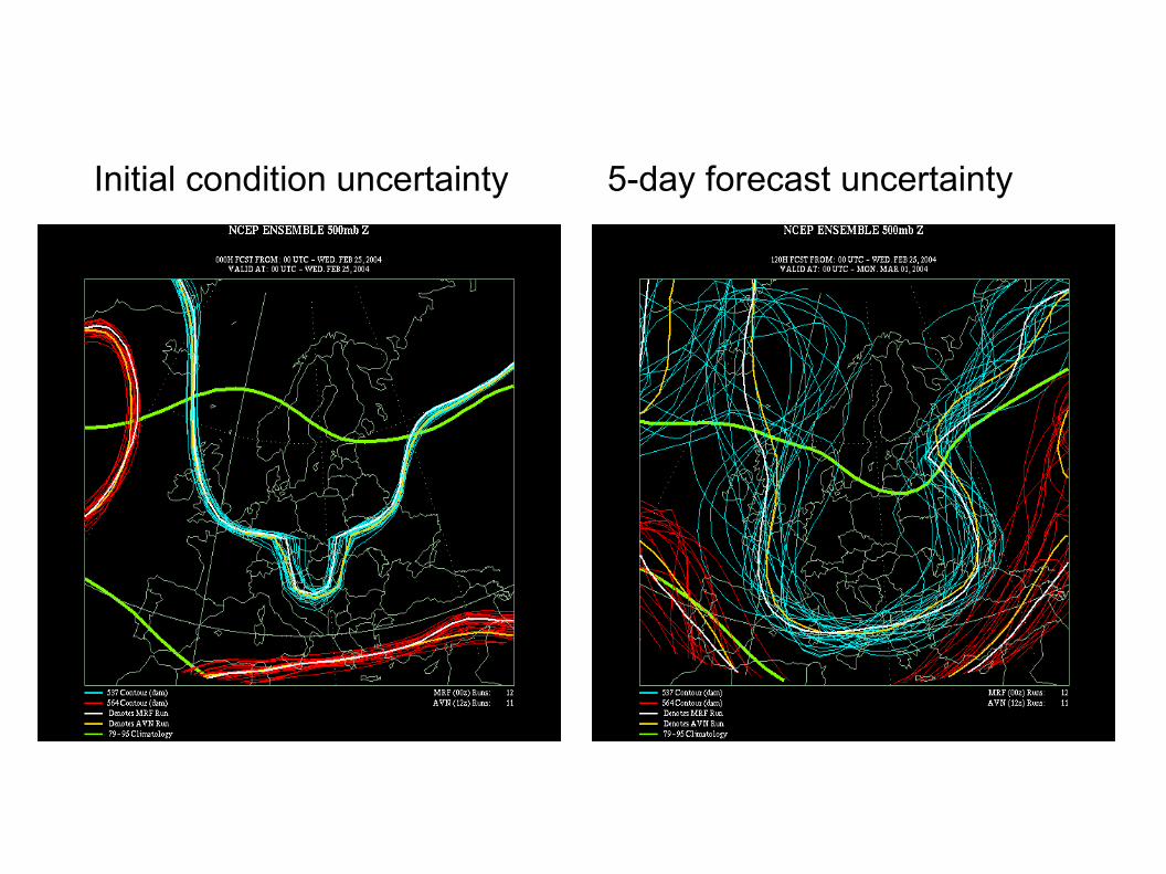
● Dynamic ● Continuous● Deterministic → Stochastic
Nonliearity in differential equations
Chaos
Limited predictability

Initial condition uncertainty 5-day forecast uncertainty

Properties of Atmospheric Models● The System:

Properties of Atmospheric Models
● Dynamic ● Continuous● Deterministic → Stochastic● Complex System

A Brief History
Early 20th Centary● Bjerknes, Vilhelm (Norwegian scientist)
– 7 primitive equations– Weather can be predicted through
computation. (1904)– Graphic calculus: solve equations
through weather maps.

A Brief History (2)
Early 20th Centary (1922)● Richardson, Lewis Fry
– First numerical weather prediction (NWP) system
– Calculating techniques: division of space into grid cells, finite difference solutions of DEs
– Forecast Factory: 64,000 computers (people who do computations), each one will perform part of the calculation.

A Brief History (3)
Computer Age (1946~)
● von Neumann and Charney– Applied ENIAC to weather prediction
● Carl-Gustaf Rossby– The Swedish Institute of Meteorology– First routine real-time numerical
weather forecasting. (1954) ( US in 1958, Japan in 1959 )

Primitive Equations
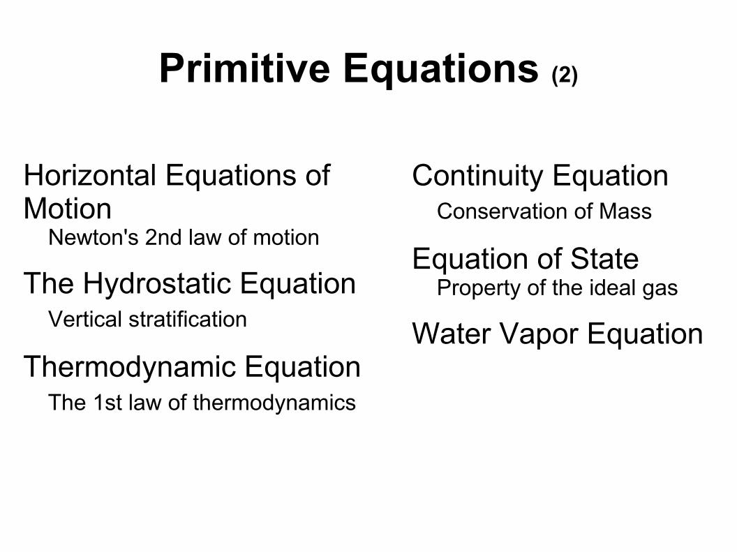
Primitive Equations (2)
Horizontal Equations of Motion Newton's 2nd law of motion
The Hydrostatic Equation Vertical stratification
Thermodynamic Equation The 1st law of thermodynamics
Continuity Equation Conservation of Mass
Equation of State Property of the ideal gas
Water Vapor Equation
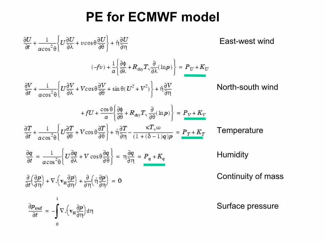
PE for ECMWF modelEast-west wind
North-south wind
Temperature
Humidity
Continuity of mass
Surface pressure

● Simplify systems– Add extra assumptions, e.g.,
● barotropic model, ● quasi-geostraphic model.
● Increase computing power– Improved numerical methods– Parallel computing

A Brief History (4)
● Norman Phillips – First general circulation model (GCM, 1955)
● Primitive equation (PE) models (late '50s ~ '70)
● 1980s : Interaction with other systems (e.g. ocean, land surface...etc.)

Properties of Atmospheric Models● The System:

System of Atmospheric Models
Atmospheric Model(dynamic, cloud, precipitation )
solar heating, long-wave cooling.....
Ocean model, plant surface model...
Forcing
Coupling
Exchanging heat, momentum and energy
Adding extra energy

Various Atmospheric Models
Complexity
ResolutionComputing Power Required
Theoretical Models
Earth System
Operational Models
Coupled Models

OutlineOutline● Properties of Atmospheric Models● A Brief History● Numerical Weather Prediction (NWP)
– Parameterization– Data Assimilation– Stochastic Weather Models
Parameterization● What is parameterization?
– Use parameters to represent sub-grid scale properties.
● Why use parameterization?– Make computation doable, both on computing
power and numerical stability.
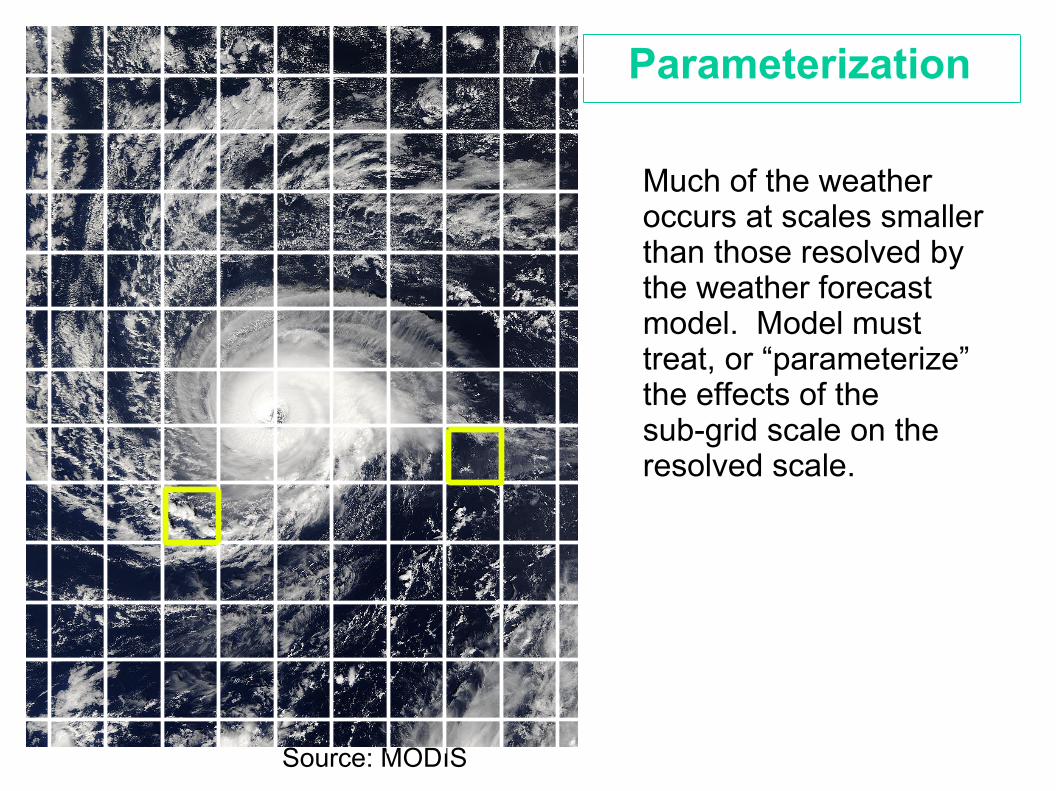
Parameterization
Much of the weather occurs at scales smallerthan those resolved bythe weather forecast model. Model musttreat, or “parameterize” the effects of the sub-grid scale on the resolved scale.
Source: MODIS

A lot happens inside a grid box
Approximatesize of one grid box in NCEP ensemble system
Source: accessmaps.com
Denver
Rocky Mountains
Systems to be Parameterized
● Land surface● Cloud micro-physics● Turbulent diffusion and interactions with surface
● Orographic drag● Radiative transfer
Parameterization Example
1.Build a detailed cloud model from observation.2.Build a classifier for its output as a function with limited complexity.
3.Use this function in a mature regional/global model.
4.Repeat step 1 ~ 3 till satisfied.
Cloud Micro-physics

NWP Flowchart

Data Assimilation
Data assimilation is the process through which real world observations:
● Enter the model's forecast cycles● Provide a safeguard against model error growth● Contribute to the initial conditions for the next
model run

Data Assimilation (2)
A model analysis is not made from observations alone. Rather, observations are used to make SMALL corrections to a short-range forecast, which is assumed to be good.
Example:● Obs. at 09:00 -> initial condition for a 3-hr
forecast.● At 12:00, new obs. is corrected by the forecast
done at 09:00, and then used for correcting the forecast for next 3-hr.
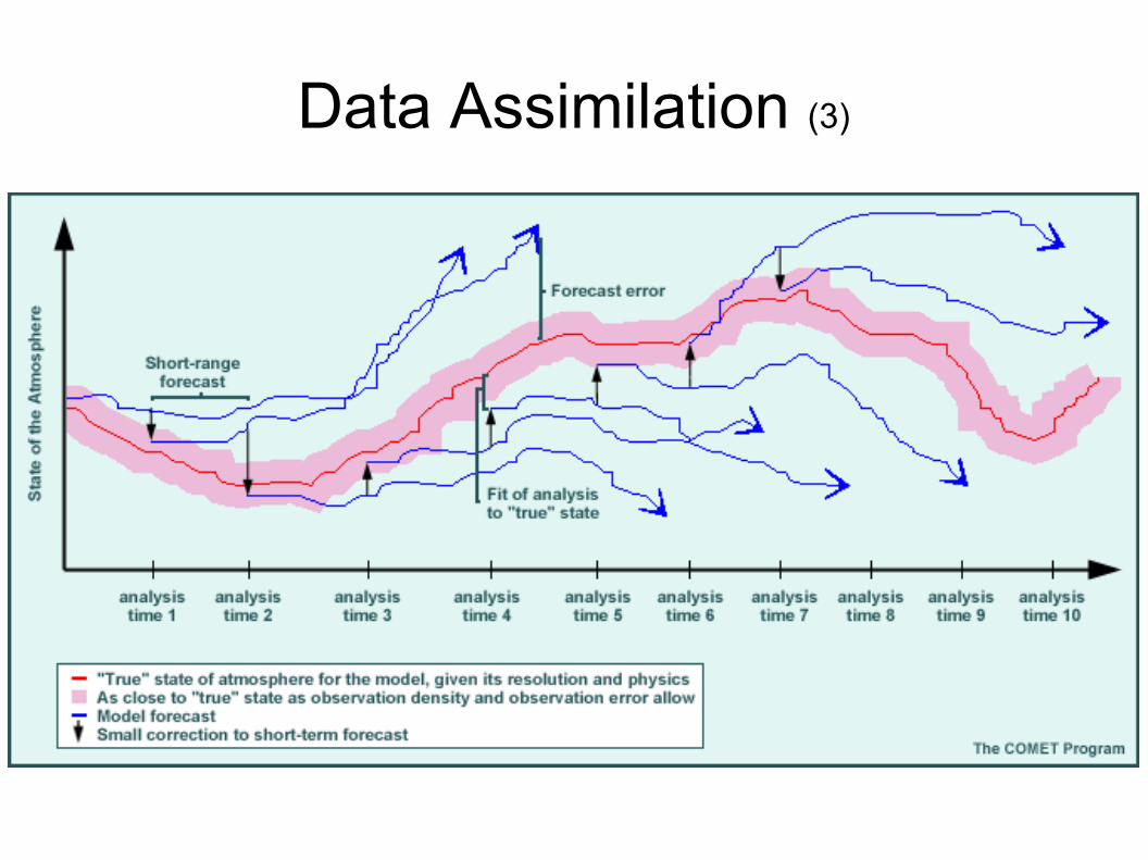
Data Assimilation (3)

Data Assimilation Procedure● Ingesting the data● Decoding coded observations● Weeding out bad data● Comparing the data to the model's short-range
"first-guess" fields● Interpolating the data (in the form of model
corrections) onto the model grid for making the forecast

Data Assimilation Procedure
Two Fundamental Difficulties in Data Assimilation
● Transferring information from the scattered locations and times of the observations to the model grid, while at the same time.
● Preserving the interrelated physical, dynamical, and numerical consistency in the short-range forecast, since these are essential to making consistently good NWP forecasts
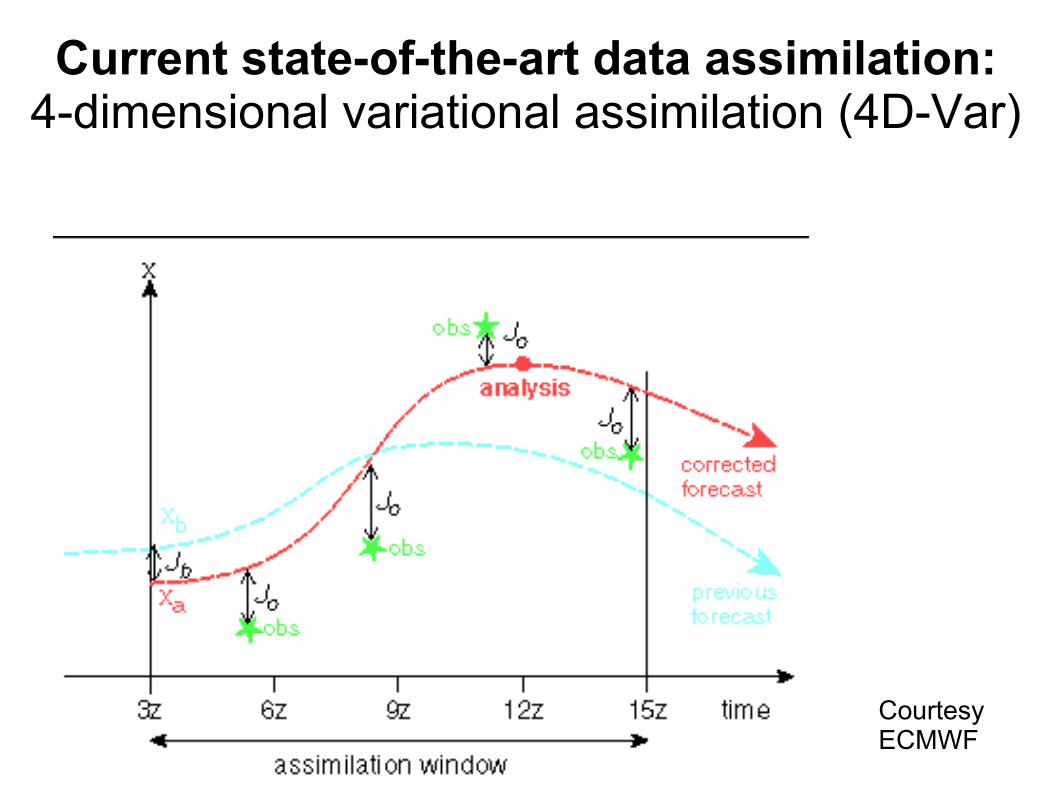
Current state-of-the-art data assimilation:4-dimensional variational assimilation (4D-Var)
CourtesyECMWF
4D-VAR● Introduced in November 1997● The influence of an observation in space and
time is controlled by the model dynamics which increases its realism of the spreading out of the information.
● The algorithm is designed to find a compromise between the previous forecast at the beginning of the time window, the observations, and the model evolution inside the time window.

Stochastic Weather Models● Stochastic-dynamic approach (climate prediction)
- Ensemble of multiple models- Stochastic differential equations
● Pure probabilistic approachFor events hardly sketch by dynamics (e.g. precipitation)
Initial condition uncertainty 5-day forecast uncertainty

Ensemble forecasts
● Generating initial conditions: Each center has adopted their own approximate way of sampling from initial condition pdf.● Breeding (NCEP)● Singular vector (ECMWF)● Perturbed observation (Canada)
● Stochastic-dynamic ensemble work just beginning (e.g., Buizza et al. 1999)
● Many attempts to post-process ensemble forecasts to provide reliable probability forecasts.
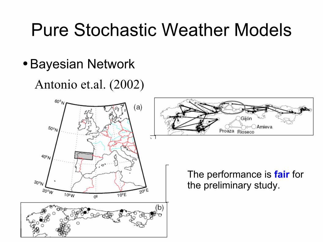
Pure Stochastic Weather Models● Bayesian Network
Antonio et.al. (2002)
The performance is fair for the preliminary study.

Conclusion● Dynamic, continuous, and deterministic models● Early development:
– Dynamic equations– Numerical methods
● Recent development:– Parameterization– Data assimilation– Probabilistic (stochastic) approach

Questions?

Reference● P. N. Edwin, A Brief History of Atmospheric General Ciculation Modeling. General Circulation
Model Development: Past, Present and Future, D. Randall, ed. (Academic Press, San Diego, 2000), pp. 67-90.
● A. Arakawa, Future Development of General Circulation Models. General Circulation Model Development: Past, Present and Future, D. Randall, ed. (Academic Press, San Diego, 2000), pp. 721-780.
● T. N. Krishnamurti and L. Bounoua, An Introduction to Numerical Weather Prediction Techniques. CRC Press, Boca Raton, 1996, pp. 121-150.
● J. R. Holton, An introduction to dynamic meteorology. (3rd Edition). International Geophysics Series, Academic Press, San Diego, 1992.
● Wilks, D. S., and R. L. Wilby 1999 The weather generation game: a review of stochastic weather models. Progr. Phys. Geogr., 23, 329—357.
● Antonio S. Cofiño, R. Cano, C. Sordo, José Manuel Gutiérrez: Bayesian Networks for Probabilistic Weather Prediction. ECAI 2002: 695-699

Okay. So how's NWP work? 1. First settle on the area to be looked at and define a grid with
an appropriate resolution.
2. Then gather weather readings for each grid point (temperature, humidity, barometric pressure, wind speed and direction, precipitation, etc.) at a number of different altitudes;
3. run your assimilation scheme to initialize the data so it fits your model;
4. now run your model by stepping it forward in time -- but not too far;
5. and go back to Step 2 again.
6. When you've finally stepped forward as far as the forecast outlook, publish your prediction to the world.
7. And finally, analyze and verify how accurately your model predicted the actual weather and revise it accordingly.

Is the weather even predictable or is the atmosphere chaotic?
That's a loaded question. We all know that weather forecasters are right only part of the time, and that they often give their predictions as percentages of possibilities. So can forecasters actually predict the weather or are they not doing much more than just playing the odds?
Part of the answer appears trivially easy -- if the sun is shining and the only clouds in the sky are nice little puffy ones, then even we can predict that the weather for the afternoon will stay nice -- probably. So of course the weathermen are actually doing their jobs (tho' they do play the odds).
But in spite of the predictability of the weather -- at least in the short-term -- the atmosphere is in fact chaotic, not in the usual sense of "random, disordered, and unpredictable," but rather, with the technical meaning of a deterministic chaotic system, that is, a system that is ordered and predictable, but in such a complex way that its patterns of order are revealed only with new mathematical tools.
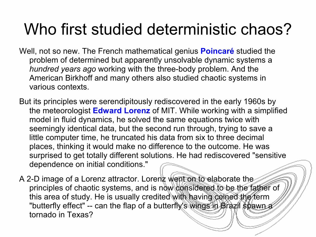
Who first studied deterministic chaos?Well, not so new. The French mathematical genius Poincaré studied the
problem of determined but apparently unsolvable dynamic systems a hundred years ago working with the three-body problem. And the American Birkhoff and many others also studied chaotic systems in various contexts.
But its principles were serendipitously rediscovered in the early 1960s by the meteorologist Edward Lorenz of MIT. While working with a simplified model in fluid dynamics, he solved the same equations twice with seemingly identical data, but the second run through, trying to save a little computer time, he truncated his data from six to three decimal places, thinking it would make no difference to the outcome. He was surprised to get totally different solutions. He had rediscovered "sensitive dependence on initial conditions."
A 2-D image of a Lorenz attractor. Lorenz went on to elaborate the principles of chaotic systems, and is now considered to be the father of this area of study. He is usually credited with having coined the term "butterfly effect" -- can the flap of a butterfly's wings in Brazil spawn a tornado in Texas?

Characteristics of a chaotic system
Deterministic chaotic behavior is found throughout the natural world -- from the way faucets drip to how bodies in space orbit each other; from how chemicals react to the way the heart beats; from the spread of epidemics of disease to the ecology of predator-prey relationships; and, of course, in the dynamics of the earth's atmosphere.

Characteristics of a chaotic system (2)
Sensitive dependence on initial conditions -- starting from extremely similar but slightly different initial conditions they will rapidly move to different states. From this principle follow these two:
* exponential amplification of errors -- any mistakes in describing the initial state of a system will therefore guarantee completely erroneous results; and
* unpredictability of long-term behavior -- even extremely accurate starting data will not allow you to get long-term results: instead, you have to stop after a bit, measure your resulting data, plug them back into your model, and continue on.
Local instability, but global stability -- in the smallest scale the behavior is completely unpredictable, while in the large scale the behavior of the system "falls back into itself," that is, restabilizes.
Aperiodic -- the phenomenon never repeats itself exactly (tho' it may come close).
Non-random -- although the phenomenon may at some level contain random elements, it is not essentially random, just chaotic.
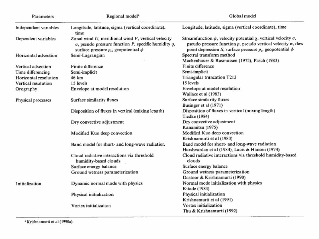
How many models are there?
Today, worldwide, there are at least a couple of dozen computer forecast models in use. They can be categorized by their:
● resolution;● outlook or time-frame -- short-range, meaning
one to two days out, and medium-range going out from three to seven days; and
● forecast area or scale -- global (which usually means the Northern hemisphere), national, and relocatable.

How good are these models and the predictions based on them?
The short answer is, Not too bad, and a lot better than forecasting without them. The longer answer is in three parts:
* Some of the models are much better at particular things than others; for example, as the USA Today article points out, the AVN "tends to perform better than the others in certain situations, such as strong low pressure near the East Coast," and "the ETA has outperformed all the others in forecasting amounts of precipitation." For more on this subject, here's a slide show from NCEP.
* The models are getting better and better as they are validated, updated, and replaced -- the "new" MRF has replaced the old (1995), and the ETA is replacing the NGM.
* That's why they'll always need the weather man -- to interpret and collate the various computer predictions, add local knowledge, look out the window, and come up with a real forecast.