Simulation and Animation of Power Electronics and Electrical Drives

Caspoc from ScratchAn Engineers workbook

Easy access to the key functions Clear Concise examples Jumpstart into simulation

INTRODUCTION..............................................................................................4

THE VERY BASICS.........................................................................................5

SETTING THE MYDOCUMENTS DIRECTORY..............................................7

MULTIPLE SIMULATIONS WITH PARAMETER VARIATIONS.....................8

IDEAL SEMICONDUCTOR PARAMETERS.................................................13

.MODEL DATABASE.....................................................................................15

CREATE A REPORT FROM YOUR SIMULATION.......................................17

CREATE A CSCRIPT....................................................................................18

SHARE VARIABLES AMONG CSCRIPTS...................................................19

HEATSINK MODELING.................................................................................21

USER DEFINED FUNCTIONS.......................................................................22

STORE FILES RELATED TO A PROJECT..................................................23

MODELING LANGUAGE IN C CODE...........................................................25

GENERATE AUTO HTML REPORTS...........................................................29

SIMULINK – CASPOC COUPLING...............................................................30

SMALL SIGNAL ANALYSIS.........................................................................34

COUPLING TO SPICE...................................................................................37

EXPORT EMBEDDED C CODE FROM THE BLOCK DIAGRAM.................38

CALCULATING PARASITIC INDUCTANCE IN COMPARE.........................39

TIPS AND TRICK FOR SPICE......................................................................40

THERMAL MODELING..................................................................................41

NUMERICAL METHODS...............................................................................42

PUBLICATIONS............................................................................................43

MODELING ELECTRICAL DRIVES..............................................................44

APPENDIX.....................................................................................................45

Cscript sample programs......................................................................................................................45

Introduction

The applications notes in this book will guide you through the process of modeling and simulation in CaspocTheir sole purpose is to guide you on your way exploring the possibilities of the program. You can read them to get a general overview of the possibilities of Caspoc or use them as a reference during your own simulation projects.

Each chapter is written to stand on its own. We recommend you to first read or follow our “Getting Started” guide, to get acquainted with the program. This will take you about 15-30 minutes, but covers most of the topics. The topics on these chapters are advanced topics, which could be useful during your won modeling and simulation projects.Also the FAQ list on www.caspoc.com gives answers to many of your questions.

The very basics

Although explained in the “Getting Started” guide, we will give a brief resume of the basic operations in CaspocBoth the circuit and the block-diagram are drawn in the same schematic. So your model contains the electric circuit, the control, the electrical load or electrical machine, plus an eventually mechanical system in one workspace.The difference between the electric circuit and the block-diagram models is indicated by the appearance of the nodes.

Electric circuitIn the electric circuit you can model your power circuit and calculate voltages over components or between nodes and currents through components. The nodes are indicated by round dots.One node should be assigned to be the reference ground node, which always has a voltage level of 0 volts. Caspoc automatically inserts a ground label, which you can replace afterwards. By clicking the node with the right-mouse button, a dialog box pops up where you can type the label of the node. For a ground reference label type “0” or “ground”. To remove the label, press the [DEL] key.

Block-diagramIn the block-diagram you can model a dynamic system by using blocks which perform an operation on the inputs of the block. For example, an “ADD” block would add the signals at the two inputs and the result is available at the output. Block-diagram blocks are always operating from the inputs to the output and are automatically sorted by Caspoc. The nodes in the block-diagram are indicated by square dots.

Connection between the circuit and the block-diagramYou can measure voltages and currents from the electric circuit using the blocks “VOLTAGE” and “CURRENT” or one of the probes from the library.Using the controlled voltage source “B” or controlled current source “A” a signal from the block diagram is used a current or voltage in the electric circuit.

Getting outputUse the “Scope” block to display any voltage, current, or block-diagram signal. You can insert a “Scope” in by clicking the first button on the bottom button bar.

And place the input of the “Scope” right on top of a circuit or block-diagram node. You can resize the “Scope” by clicking and dragging the right-bottom corner. The number of inputs automatically increases while resizing the “Scope”.

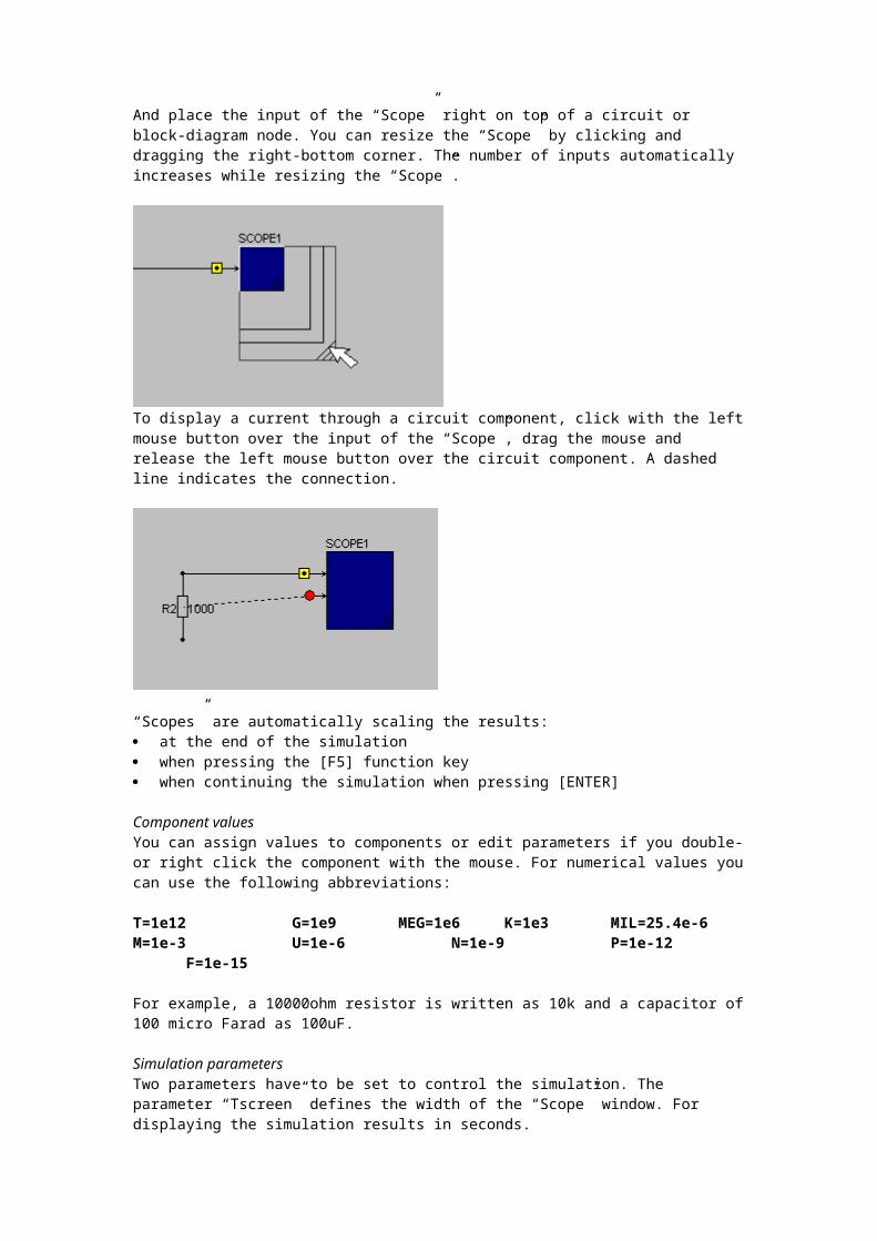
To display a current through a circuit component, click with the left mouse button over the input of the “Scope”, drag the mouse and release the left mouse button over the circuit component. A dashed line indicates the connection.

“Scopes” are automatically scaling the results: at the end of the simulation when pressing the [F5] function key when continuing the simulation when pressing [ENTER]

Component valuesYou can assign values to components or edit parameters if you double- or right click the component with the mouse. For numerical values you can use the following abbreviations:

T=1e12 G=1e9 MEG=1e6 K=1e3 MIL=25.4e-6M=1e-3 U=1e-6 N=1e-9 P=1e-12 F=1e-15

For example, a 10000ohm resistor is written as 10k and a capacitor of 100 micro Farad as 100uF.

Simulation parametersTwo parameters have to be set to control the simulation. The parameter “Tscreen” defines the width of the “Scope” window. For displaying the simulation results in seconds.

The parameter “dT” defines the integration time step. As rule of thumb you can set it to approximately 1/10 to 1/00 of the reciprocal of the highest frequency occurring in your simulation. For example, use dT=100us and Tscreen=100ms for a line commutated converter operating a 50Hz or at 60Hz, or set dT=1us and Tscreen to 1ms for a Switched-Mode Power Supply operating at 10kHz.

Starting the simulation

Start the simulation by pressing the “Play” button or pressing the [Enter] key.

You can vary parameters during the simulation and simply continue by selecting the pause/continue button, or pressing the [Enter] key.

Now that you understand the basic commands of the program, you are ready to start your own simulation projects.

Basic topic

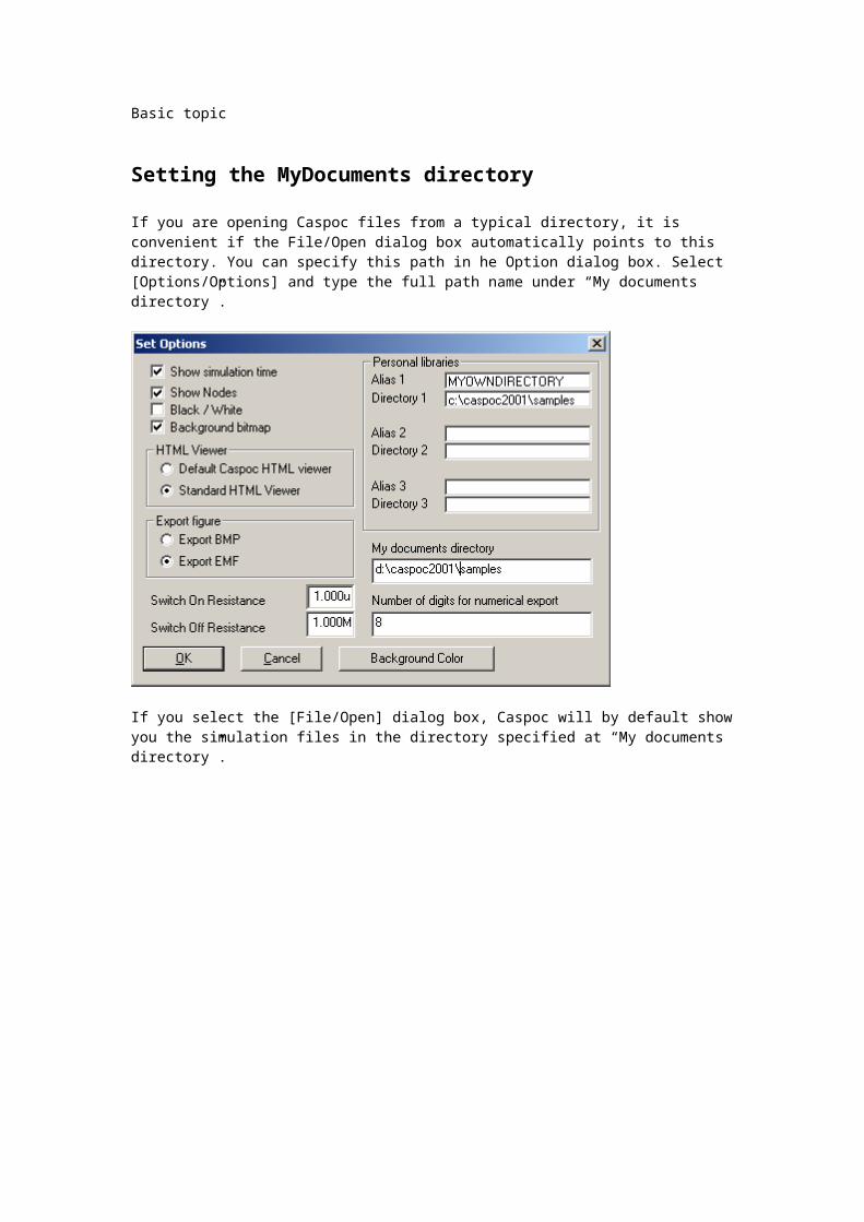
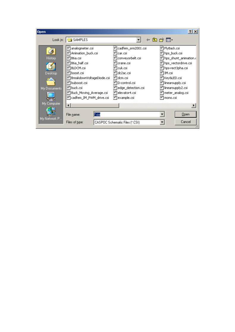
Setting the MyDocuments directory

If you are opening Caspoc files from a typical directory, it is convenient if the File/Open dialog box automatically points to this directory. You can specify this path in he Option dialog box. Select [Options/Options] and type the full path name under “My documents directory”.

If you select the [File/Open] dialog box, Caspoc will by default show you the simulation files in the directory specified at “My documents directory”.

Advanced Topic

Multiple simulations with parameter variations

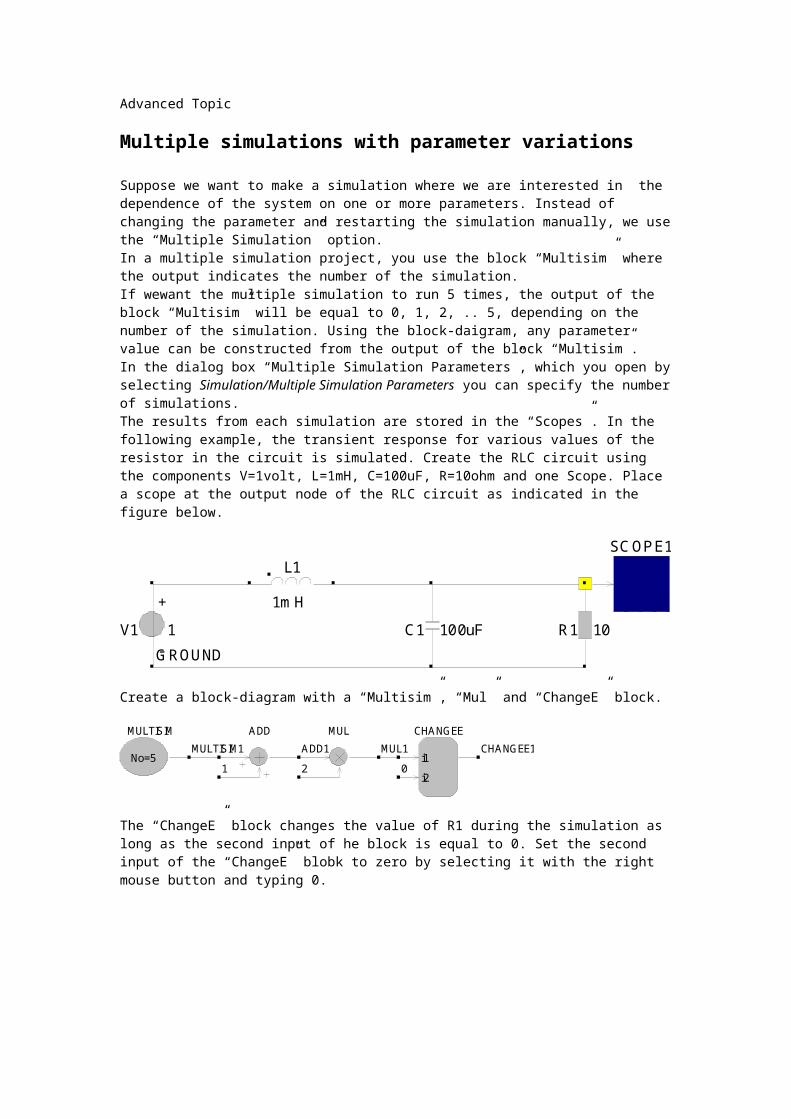
Suppose we want to make a simulation where we are interested in the dependence of the system on one or more parameters. Instead of changing the parameter and restarting the simulation manually, we use the “Multiple Simulation” option.In a multiple simulation project, you use the block “Multisim” where the output indicates the number of the simulation.If wewant the multiple simulation to run 5 times, the output of the block “Multisim” will be equal to 0, 1, 2, .. 5, depending on the number of the simulation. Using the block-daigram, any parameter value can be constructed from the output of the block “Multisim”.In the dialog box “Multiple Simulation Parameters”, which you open by selecting Simulation/Multiple Simulation Parameters you can specify the number of simulations.The results from each simulation are stored in the “Scopes”. In the following example, the transient response for various values of the resistor in the circuit is simulated. Create the RLC circuit using the components V=1volt, L=1mH, C=100uF, R=10ohm and one Scope. Place a scope at the output node of the RLC circuit as indicated in the figure below.

V1 1 +

-

L1

1mH

C1 100uF R1 10

SCOPE1

GROUND

Create a block-diagram with a “Multisim”, “Mul” and “ChangeE” block.

CHANGEE

i1

i2

MULTISIM

No=5

MULADD

0

CHANGEE1MULTISIM1 MUL1ADD1

21

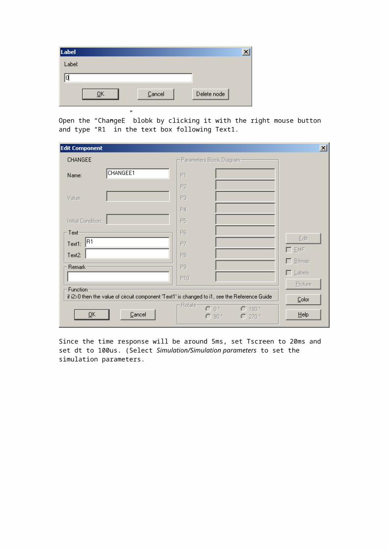
The “ChangeE” block changes the value of R1 during the simulation as long as the second input of he block is equal to 0. Set the second input of the “ChangeE” blobk to zero by selecting it with the right mouse button and typing 0.

Open the “ChangeE” blobk by clicking it with the right mouse button and type “R1” in the text box following Text1.

Since the time response will be around 5ms, set Tscreen to 20ms and set dt to 100us. (Select Simulation/Simulation parameters to set the simulation parameters.

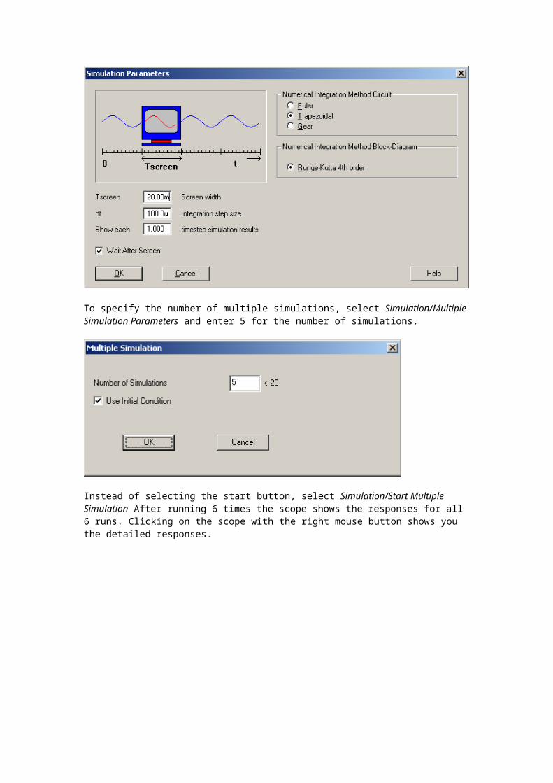
To specify the number of multiple simulations, select Simulation/Multiple Simulation Parameters and enter 5 for the number of simulations.

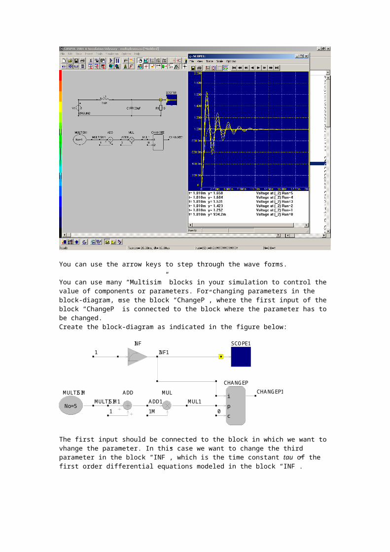
Instead of selecting the start button, select Simulation/Start Multiple Simulation After running 6 times the scope shows the responses for all 6 runs. Clicking on the scope with the right mouse button shows you the detailed responses.

You can use the arrow keys to step through the wave forms.

You can use many “Multisim” blocks in your simulation to control the value of components or parameters. For changing parameters in the block-diagram, use the block “ChangeP”, where the first input of the block “ChangeP” is connected to the block where the parameter has to be changed.Create the block-diagram as indicated in the figure below:

SCOPE1

MULTISIM

No=5

MULADD

CHANGEP

i

p

c

INF

MULTISIM1 MUL1ADD1

1M1

CHANGEP1

0

1 INF1

The first input should be connected to the block in which we want to vhange the parameter. In this case we want to change the third parameter in the block “INF”, which is the time constant tau of the first order differential equations modeled in the block “INF”.

The second input is the new value, which we want to place in the block “INF” using the “ChangeP” block. Set the third input to 0, so Caspoc will automatically determine when to change the parameter. To indicate which parameter to change in the block connected to the first input of the block “ChangeP”, we have to specify the parameter p(n) in the block “ChangeP”. Since we want to change the third parameter tau, specify 3.

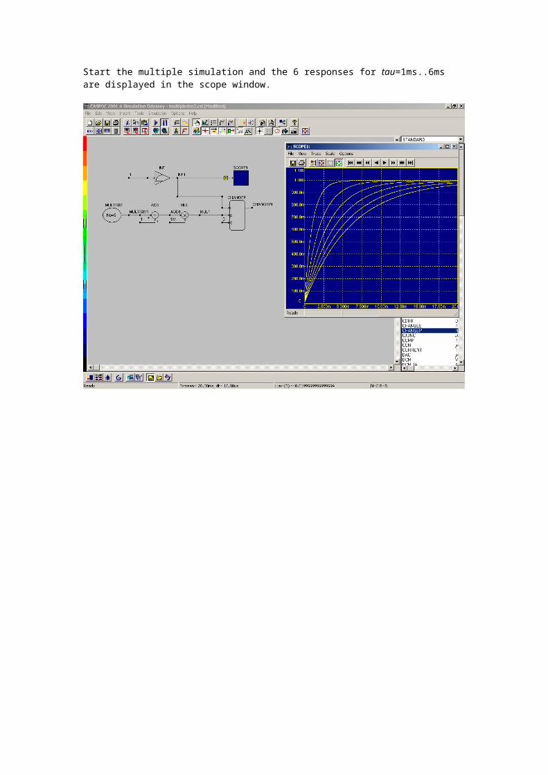
Start the multiple simulation and the 6 responses for tau=1ms..6ms are displayed in the scope window.

Advanced Topic

Ideal semiconductor parameters

The ideal semiconductor parameters are optimized for a high simulation speed and no convergence problems.You can set these parameters by using the “.Model” library.In the properties dialog box for a diode (Select it by right clicking the diode), you can specify the name of the “.Model”. As default the model “Diode” is used for the ideal switch model of the diode

Type here for example “MyModel”

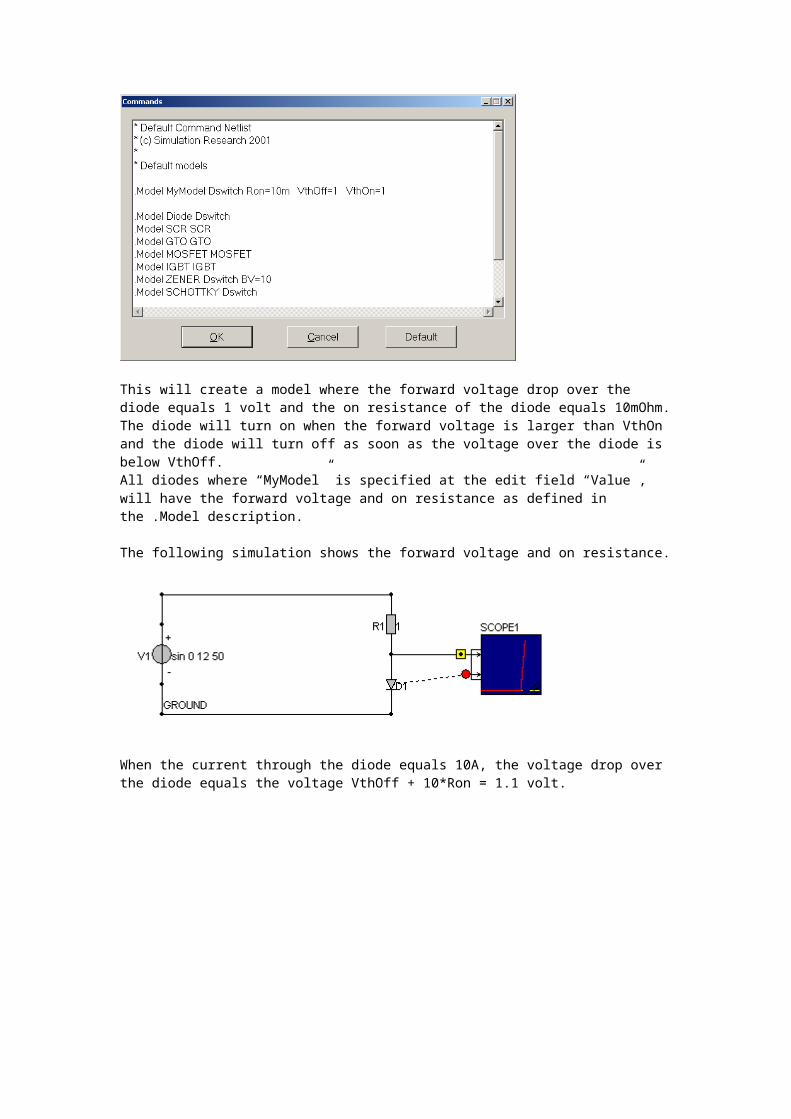
Secondly you have to define your new “MyModel”. Therefore you open the dialog box for the commands by selecting “Insert/Edit Commands”. In the edit field, add the following line:.Model MyModel Dswitch Ron=10m VthOff=1 VthOn=1

This will create a model where the forward voltage drop over the diode equals 1 volt and the on resistance of the diode equals 10mOhm. The diode will turn on when the forward voltage is larger than VthOn and the diode will turn off as soon as the voltage over the diode is below VthOff.All diodes where “MyModel” is specified at the edit field “Value”, will have the forward voltage and on resistance as defined in the .Model description.

The following simulation shows the forward voltage and on resistance.

When the current through the diode equals 10A, the voltage drop over the diode equals the voltage VthOff + 10*Ron = 1.1 volt.

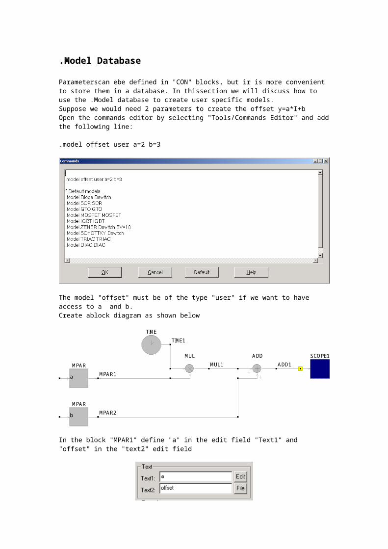
.Model Database

Parameterscan ebe defined in "CON" blocks, but ir is more convenient to store them in a database. In thissection we will discuss how to use the .Model database to create user specific models.Suppose we would need 2 parameters to create the offset y=a*I+bOpen the commands editor by selecting "Tools/Commands Editor" and add the following line:

.model offset user a=2 b=3

The model "offset" must be of the type "user" if we want to have access to a and b.Create ablock diagram as shown below

SCOPE1ADD

TIME

MUL

MPAR

b

MPAR

a

ADD1

TIME1

MUL1

MPAR2

MPAR1

In the block "MPAR1" define "a" in the edit field "Text1" and "offset" in the "text2" edit field

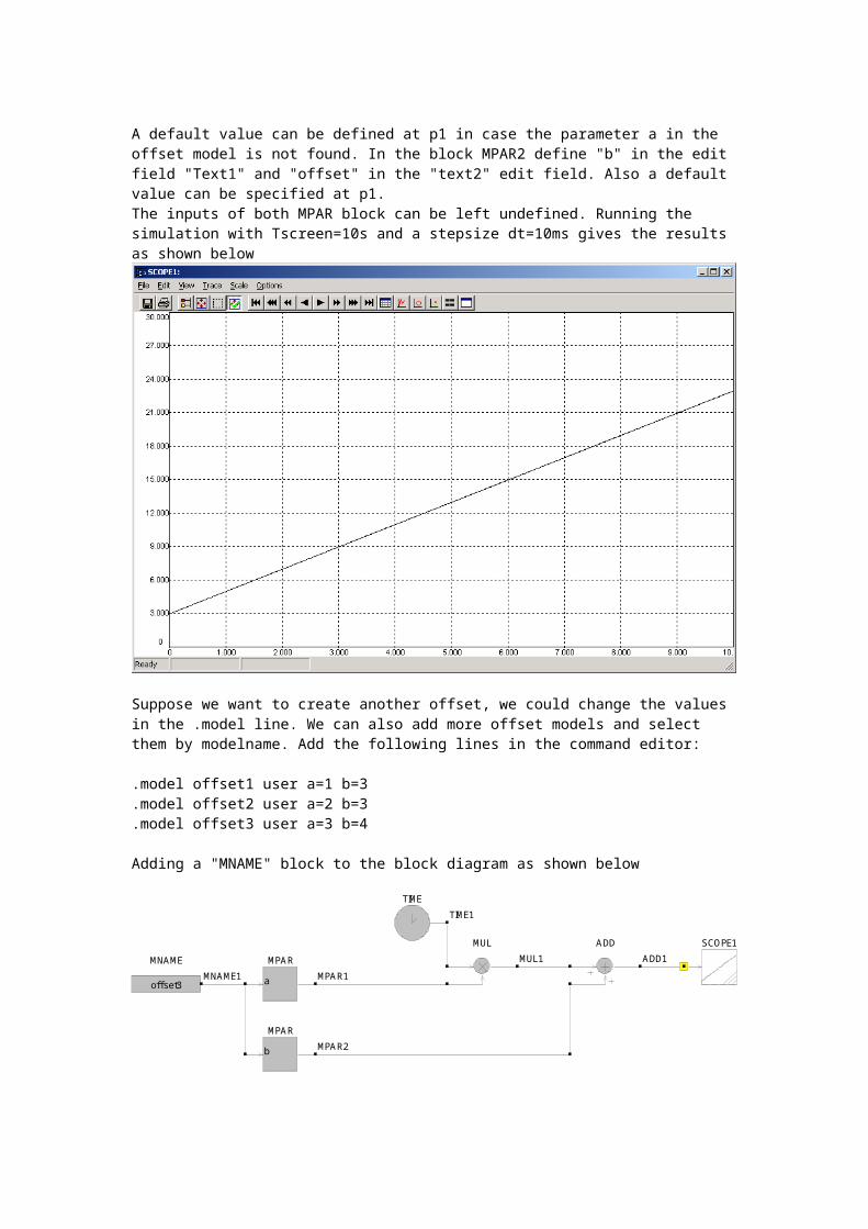
A default value can be defined at p1 in case the parameter a in the offset model is not found. In the block MPAR2 define "b" in the edit field "Text1" and "offset" in the "text2" edit field. Also a default value can be specified at p1.The inputs of both MPAR block can be left undefined. Running the simulation with Tscreen=10s and a stepsize dt=10ms gives the results as shown below

Suppose we want to create another offset, we could change the values in the .model line. We can also add more offset models and select them by modelname. Add the following lines in the command editor:

.model offset1 user a=1 b=3

.model offset2 user a=2 b=3

.model offset3 user a=3 b=4

Adding a "MNAME" block to the block diagram as shown below

MNAME

offset3

SCOPE1ADD

TIME

MUL

MPAR

b

MPAR

aMNAME1

ADD1

TIME1

MUL1

MPAR2

MPAR1

Starting the simulation with Tscreen=10 and dt=10ms gives the offset specified by model offset3. By changing the model name in the "text1" edit field in the block"MNAME", changes the user model.

Create a report from your simulation

Caspoc has a build in report generator to create internet-enabled reports from yopur simulation. After finishing your simulations, select "Tools/Export HTML" for creating your report.

Fill the edit fields with:a) The title of your reportb) Component detailsc) Remarks

Select the [Export] button to create your report. The report will be saved under the same filename as your simulation file, with the .html extension. The worksscreen (schematic) will be saved as an Enhanced Meta File (EMF) with the .emf exension. All scope output will be saved with the extension .scopei.emf

You can use HTML editing commands for formatting the text in your report:

<b>bold</b> b<i>italic</i> ix² x2

x₀ x0

You can use tables or ordered lists in the HTML format.

<table><tr><td>R</td><td>1 ohm</td></tr><tr><td>C</td><td>10mF</td></tr><tr><td>L</td><td>10nH</td></tr></table>

<ol><li>remark 1</li><li>remark 2</li><li>remark 3</li>

</ol>

Create a Cscript

For complex models or modeling a control the Cscript block allows you to create your own blocks.The function of the block is defined by ANSI-C code, see the appendix for the details on the syntax.The input for the block Cscript is "a" and is defined as a local "int" variable inside the scripts Main function.

12345678

int iCount;int y;main() { iCount=10; y=a+iCount; return(y); }

// Local declaration of iCount// Local declaration of y// Main function// Opening brace// Set iCount to 1// Add iCount to the input a// Set the output of the block to y// Closing brace

Local variable can be defied outside the main function as is done in lines 1 and 2. There has to be one main function with opening and closing braces, see lines 3,4 and 8. The variable a is defined as being the input of the block. It doesn’t have to be declared, as it is done automatically by Caspoc as a local variable that is defined inside the scope of the main function. The argument of the return function, in this case y in line 7, is the output of the block.

The blocks Cscript2, Cscript3, … Cscript20 have more inputs labeled from "a" until "t"

Inside the Cscript block you can use loops like for, while do and if-then-else structures. Functions can be called recursively and you can pass local variables as function arguments. Variables are declared from the type "int".

Features of Cscript include:

Parameterized functions with local variables Recursion The if statement The do-while, while, and for loops Integer and character variables Global variables Integer and character constants String constants (limited implementation) The return statement, both with and without a value A limited number of standard library functions Operators: +, -, *, / , %, <, >, <=, >=, ==, !=, unary -, unary +, *=, +=, -=, /=, &=, |= and ^= Support for && and || in comparisons Functions returning integers Comments // and /* */

Share variables among Cscripts

To exchange variables between Cscripts blocks or have more inputs and outputs, the CVAR block is used.Using the CVAR block global variables are defined that are accessible in all Cscript blocks in your simulation.

Use this block to:1. Send parameters to the Cscript blocks.2. Get numerical values from the Cscript block.3. Exchange numerical values between Cscript blocks4. Provide more inputs & outputs for the Cscript blocks.

Per global variable one CVAR is used. Define the name of the variable at the edit field "text1" of the block.

In the ANSI-C language both variables "a" and "A" can exist and have different values. In other words, "a" and "A" are not equal. At p1 in the properties you can also define the initial value. The declared variable can be used in all Cscript blocks in your simulation.

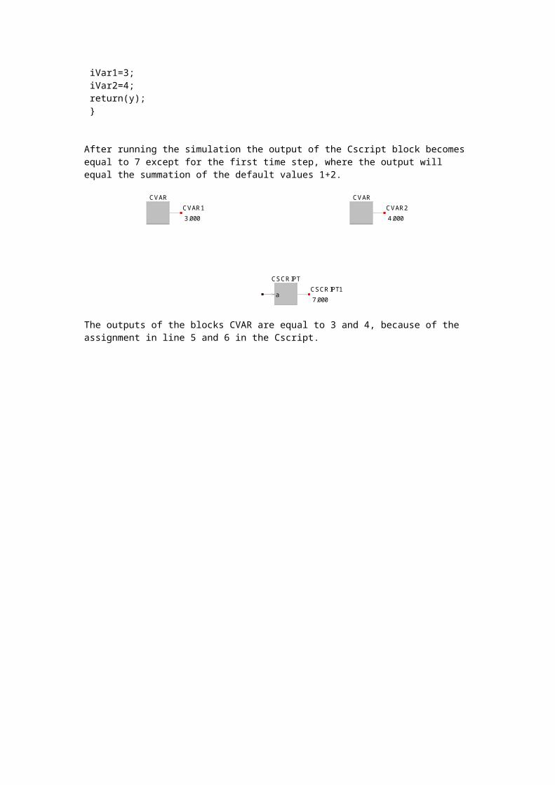
In the example below two global variables are declared: iVar1 and iVar2, both of the type integer. Their default value is set to

iVar1=1;iVar2=2;

by defining the default value at p1.

Both variables iVar1 and iVar2 are declared for all Cscripts in the simulation. In this simulation we will use the default value and replace it with a new value.In the Cscript, the value of iVar1 and iVar2 is added and returned as the output of the Cscript block. The variables iVar1 and iVar2 get a new value being:

iVar1=3;iVar2=4;

and thereby replacing the previous values. These new values are set at the outputs of the CVAR blocks.

The Cscript is shown below.

int y; main() { y=iVar1+iVar2; iVar1=3; iVar2=4; return(y); }

After running the simulation the output of the Cscript block becomes equal to 7 except for the first time step, where the output will equal the summation of the default values 1+2.

CVARCVAR

CSCRIPT

a

CVAR2CVAR1

CSCRIPT1

4.000 3.000

7.000

The outputs of the blocks CVAR are equal to 3 and 4, because of the assignment in line 5 and 6 in the Cscript.

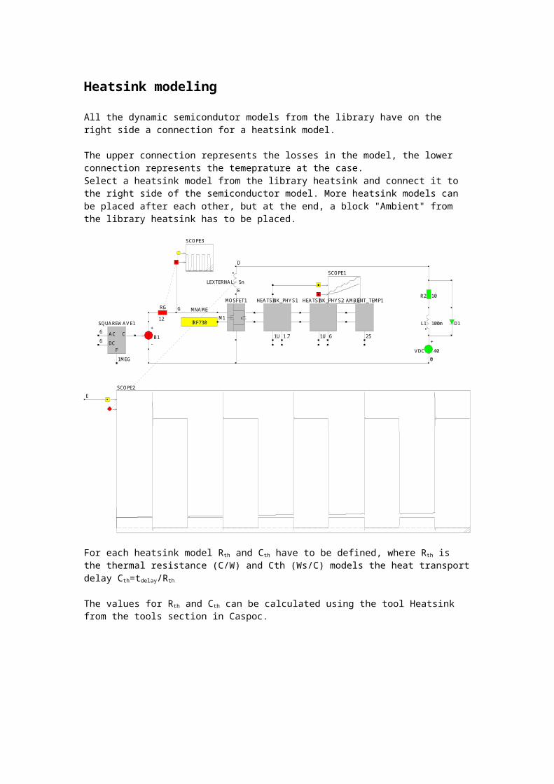
Heatsink modeling

All the dynamic semicondutor models from the library have on the right side a connection for a heatsink model.

The upper connection represents the losses in the model, the lower connection represents the temeprature at the case. Select a heatsink model from the library heatsink and connect it to the right side of the semiconductor model. More heatsink models can be placed after each other, but at the end, a block "Ambient" from the library heatsink has to be placed.

SCOPE2

SCOPE3

SCOPE1

D

MOSFET1

LEXTERNAL 5n

MNAME

IRF730

AC

DC

C

F

SQUAREWAVE1

B1+

-

R2 10

RG

12 L1 100m

VDC 40 +

-

D1

HEATSINK_PHYS2 AMBIENT_TEMP1HEATSINK_PHYS1

E

0

251.71U

M1

E

6

6

1MEG

G

D

61U

For each heatsink model Rth and Cth have to be defined, where Rth is the thermal resistance (C/W) and Cth (Ws/C) models the heat transport delay Cth=tdelay/Rth

The values for Rth and Cth can be calculated using the tool Heatsink from the tools section in Caspoc.

User defined functions

In the "Expression" block a user defiend function can be defined. This block is aimed for simple algebraic equations and is faster than the Cscript block.Depending on the number of inputs to the block, the inputs areavailable as a, b, c, d, ….Use can be made of + - / * ( ) Although supported the ^ operator can be used for raising power. However it is recommended not to use the ^ operator, since it is not supported in the ANSI-C language.To model, for example:

use the following equation and define it at the edit field text:

EXPRESSION4

a

b

c

dY2

Y1

X2

X1 EXPRESSION41

Always use enough brackets to structure your equations.

Store files related to a project

To acces various files, that belong to one project, from the project manager, you can simply put them in a directory which has the same name as the main simulation file. Both the simulation file (*.csi) and thedirectory have to reside in the same directory.For example, a project called MyProject contains one main simulation file MyProject.csi, a text file data.txt and an excel sheet calc.xls.The simulaiton file MyProject.csi is in the directory samples. Create the directory MyPorject in the directory Samples and save there the text and excel files.

[Samples]MyProject.csi[MyProject]

data.txtcalc.xls

Opening the Files section in the Project section in the project manager after opening the MyProject.csi simulation file, wil show the files and subdirectories in the Files section. You can open these files by double clicking them.

If the simulation file MyProject.csi is opened the files in the directory with the same name , in this case "MyProject", are placed in the project manager.Double click the "Projects" in the project manager and double click on "Files". All files from the directory "MyProject are listed in the project manager.

Depending on the extension of the file, the file is opened in the associated application. Files with the .dat extension are opened in the default Scope in Caspoc, where you can edit its content with the numerical table editor.

Advanced Topic

Modeling Language in C code

You can build your own blocks in C using Microsoft Visual C++ version 4.2 or higher. A template is provided which models a first order differential equation, like described in the manual. The example standardml.csi, which is provided for this template calls the modeling language file standardml.dll three times and the results are compared with the results from an INF block.You can run this example from the debugger and also put breakpoints in the source code, to debug your modeling language.

In the above figure a breakpoint is inserted when t exceeds 5seconds

The code for the above example is in the template standardml.c. Open this template by opening the standardML.mdp project workspace file. If you want to use the debugger, place you simulation file in the same directory as standardML.dll in debug mode is created. This is mostly in the debug directory, although you can change this in the options for the compiler.If you run the example from another directory where another standardML.dll is already present, the debugger will not work correctly. Remove the old standardML.dll file, before compiling a new version and debugging it in the compiler.

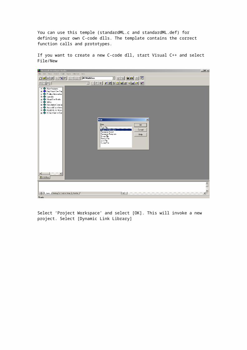
You can use this temple (standardML.c and standardML.def) for defining your own C-code dlls. The template contains the correct function calls and prototypes.

If you want to create a new C-code dll, start Visual C++ and select File/New

Select ‘Project Workspace’ and select [OK]. This will invoke a new project. Select [Dynamic Link Library]

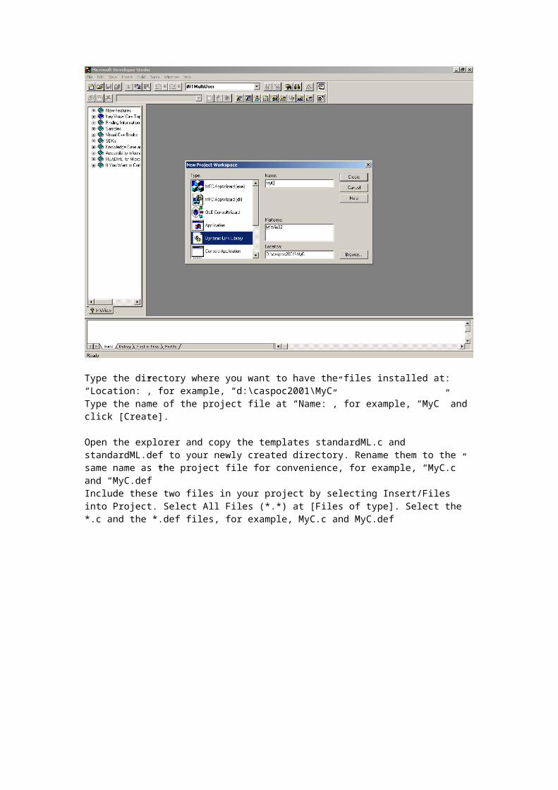
Type the directory where you want to have the files installed at: “Location:”, for example, “d:\caspoc2001\MyC”Type the name of the project file at “Name:”, for example, “MyC” and click [Create].

Open the explorer and copy the templates standardML.c and standardML.def to your newly created directory. Rename them to the same name as the project file for convenience, for example, “MyC.c” and “MyC.def”Include these two files in your project by selecting Insert/Files into Project. Select All Files (*.*) at [Files of type]. Select the *.c and the *.def files, for example, MyC.c and MyC.def

Select [Add] to include the files in your project workspace. By double clicking the files folder in the left window, you can select the *.c or the *.def files for editing. The exported function should be specified in the *.def file.

The dll, which you use during debugging, should not be used as final release. Therefore the ‘Release’ option can be set. This Release version, which runs without debugger is much faster. Set the [Release] compile option for creating your final dll in the toolbar ‘Project’.

In the project settings [Build/Settings], (ALT-F7), you can specify where the *.dll is created.

The function:

int ML_C(void){return 1;}

has to be defined to let Caspoc know that this is a C file and not a Delphi file.

The explanation of the source code for this example is found in the manual under:

User guideChapter 14: Multilevel modeling and syntax

Advanced Topic

Generate Auto HTML Reports

From each simulation you can create an HTLM report, which includes the schematic and the simulation results. Before creating the report you have to run the simulation to obtain the results.If you would need to generate a large number of reports, this could be a tedious job. Instead you can use the auto generation tool, which creates all the reports with simulations results, from all the simulations in one directory

In the edit field ‘directory’ specify the directory which contains all your simulations. Select [Start] to start the simulations and report generations.Each simulation file with the extension *.csi is opened, simulated and the report is generated. When all simulations are finished and all reports are generated, an index file is created with the name index.html. For each simulation Wait After Screen in the dialog box Simulation Parameters is enabled, so each simulation is limited to Tscreen seconds.

Advanced Topic

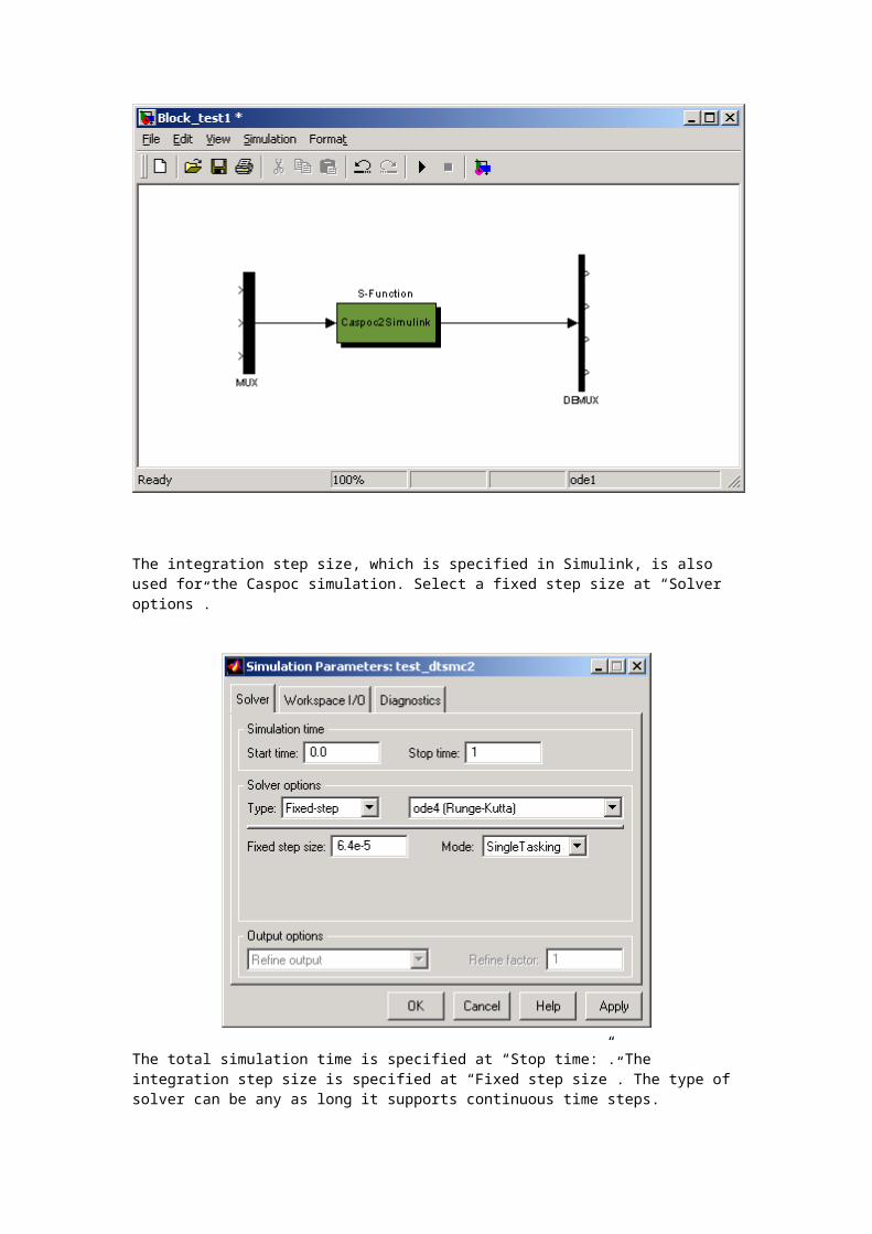
Simulink – Caspoc Coupling

You can couple the models in Caspoc and Simulink. This is advantageous when modeling power electronics, since Caspoc is better suited for modeling switching circuits, especially power electronics.

Caspoc is running in the background and data can be interchanged between Caspoc and Simulink with the use of a S-Function block.

SIMULINK:In Simulink select a S-Function block from the tree list and place it in your simulink model. Select a MUX-block and place it in front of the S-Function block. Select a DEMUX-block and place it behind the S-Function block

CASPOC:In Caspoc you use the block ToSLNK block to send data to Simulink. Use the FromSLNK block to read data from Simulink. In the ToSLNK block (first parameter), specify the number of the outputs in the DEMUX block in Simulink. In the FromSLNK block (first parameter), specify the number of the inputs in the MUX block in Simulink.

The number of ToSLNK blocks should equal the width of the DEMUX block in Simulink. Change the width of the DEMUX block by double clicking it with the left mouse button and specify the number of ToSLNK blocks.The number of FromSLNK blocks should equal the width of the MUX block in Simulink. Change the width of the MUX block by double clicking it with the left mouse button and specify the number of FromSLNK blocks.

For example, if 4 ToSLNK and 3 FromSLNK blocks are specified in Caspoc, the MUX block has 3 inputs and the DEMUX block has 4 outputs.

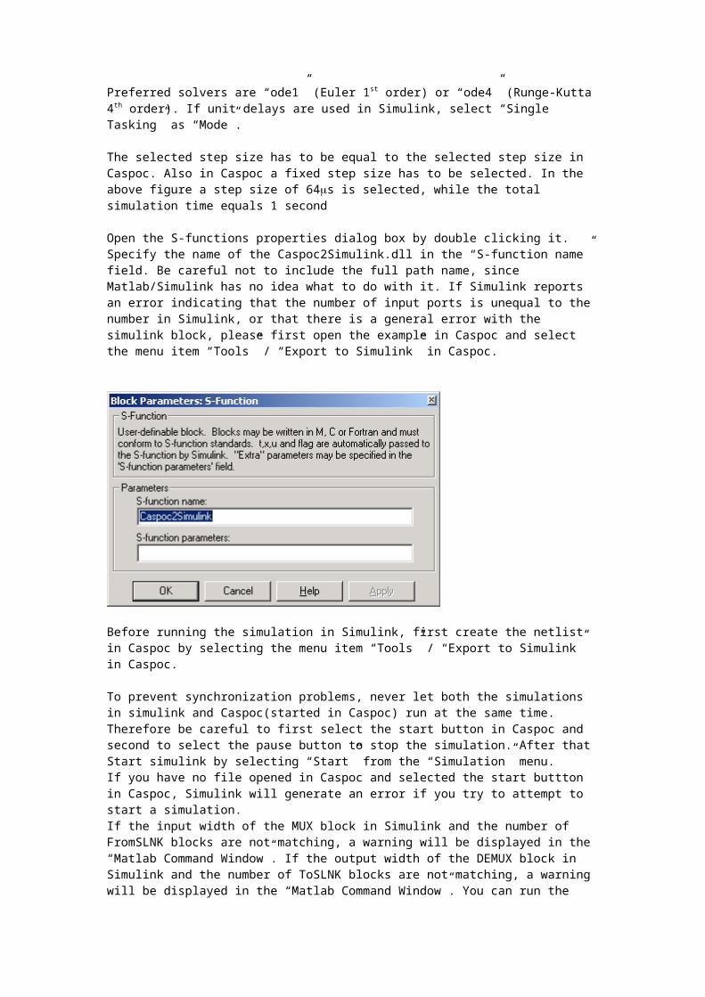
The integration step size, which is specified in Simulink, is also used for the Caspoc simulation. Select a fixed step size at “Solver options”.

The total simulation time is specified at “Stop time:”. The integration step size is specified at “Fixed step size”. The type of solver can be any as long it supports continuous time steps. Preferred solvers are “ode1” (Euler 1st order) or “ode4” (Runge-Kutta 4th order). If unit delays are used in Simulink, select “Single Tasking” as “Mode”.

The selected step size has to be equal to the selected step size in Caspoc. Also in Caspoc a fixed step size has to be selected. In the above figure a step size of 64s is selected, while the total simulation time equals 1 second

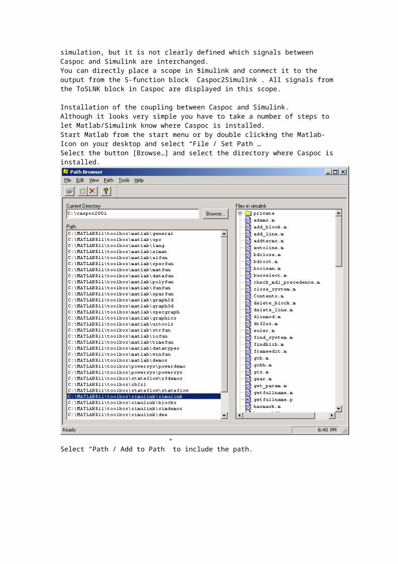
Open the S-functions properties dialog box by double clicking it. Specify the name of the Caspoc2Simulink.dll in the “S-function name” field. Be careful not to include the full path name, since Matlab/Simulink has no idea what to do with it. If Simulink reports an error indicating that the number of input ports is unequal to the number in Simulink, or that there is a general error with the simulink block, please first open the example in Caspoc and select the menu item “Tools” / “Export to Simulink” in Caspoc.

Before running the simulation in Simulink, first create the netlist in Caspoc by selecting the menu item “Tools” / “Export to Simulink” in Caspoc.

To prevent synchronization problems, never let both the simulations in simulink and Caspoc(started in Caspoc) run at the same time. Therefore be careful to first select the start button in Caspoc and second to select the pause button to stop the simulation. After that Start simulink by selecting “Start” from the “Simulation” menu.If you have no file opened in Caspoc and selected the start buttton in Caspoc, Simulink will generate an error if you try to attempt to start a simulation. If the input width of the MUX block in Simulink and the number of FromSLNK blocks are not matching, a warning will be displayed in the “Matlab Command Window”. If the output width of the DEMUX block in Simulink and the number of ToSLNK blocks are not matching, a warning will be displayed in the “Matlab Command Window”. You can run the simulation, but it is not clearly defined which signals between Caspoc and Simulink are interchanged. You can directly place a scope in Simulink and connect it to the output from the S-function block ”Caspoc2Simulink”. All signals from the ToSLNK block in Caspoc are displayed in this scope.

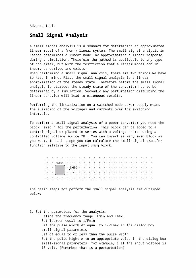
Installation of the coupling between Caspoc and Simulink.Although it looks very simple you have to take a number of steps to let Matlab/Simulink know where Caspoc is installed. Start Matlab from the start menu or by double clicking the Matlab-Icon on your desktop and select “File / Set Path …”Select the button [Browse…] and select the directory where Caspoc is installed.

Select “Path / Add to Path” to include the path.

Whenever you make a change in the Caspoc model, don’t forget to first export it for Simulink with the menu item “Tools” / “Export to Simulink” in Caspoc.

Advance Topic

Small Signal Analysis

A small signal analysis is a synonym for determining an approximated linear model of a (non-) linear system. The small signal analysis in Caspoc determines a linear model by approximating a linear response during a simulation. Therefore the method is applicable to any type of converter, but with the restriction that a linear model can in theory be derived and exists.When performing a small signal analysis, there are two things we have to keep in mind. First the small signal analysis is a linear approximation of the steady state. Therefore before the small signal analysis is started, the steady state of the converter has to be determined by a simulation. Secondly any perturbation disturbing the linear behavior will lead to erroneous results.

Performing the linearization on a switched mode power supply means the averaging of the voltages and currents over the switching intervals.

To perform a small signal analysis of a power converter you need the block “smsg “ for the perturbation. This block can be added to a control signal or placed in series with a voltage source using a controlled voltage source “B”. You can insert as many smsg block as you want. In each scope you can calculate the small-signal transfer function relative to the input smsg block.

The basic steps for perform the small signal analysis are outlined below:

1. Set the parameters for the analysis:Define the frequency range, Fmin and Fmax. Set Tscreen equal to 1/FminSet the pulse width dt equal to 1/2Fmax in the dialog box small-signal parametersSet dt equal to or less than the pulse widthSet the pulse hight A to an appropriate value in the dialog box small-signal parameters, for example, 1 if the input voltage is 10 volt. (Remember that is a perturbation)

2. Simulate the circuit until steady state.

3. Save the initial conditions in the *.ic file.

4. Start the small signal analyses by selecting the small signal start button or selecting: “Simulation/Start small signal analysis”

5. The simulation will run two times. First for the steady state and secondly for the perturbation.

6. Open the scope with the right mouse button.

7. The small signal calculation is performed automatically.

8. The number of harmonics calculated is equal to: Scale/DFT Parameters : [Number of harmonics] in the scope and is not adjusted automatically.

9. Set the number of harmonics, for example 100 or 1000 and select: View/DFT. The small-signal transfer function is recalculated and displayed

10. Each time a new small-signal analysis is carried out where one of the circuit parameters is changed, proceed with step 2

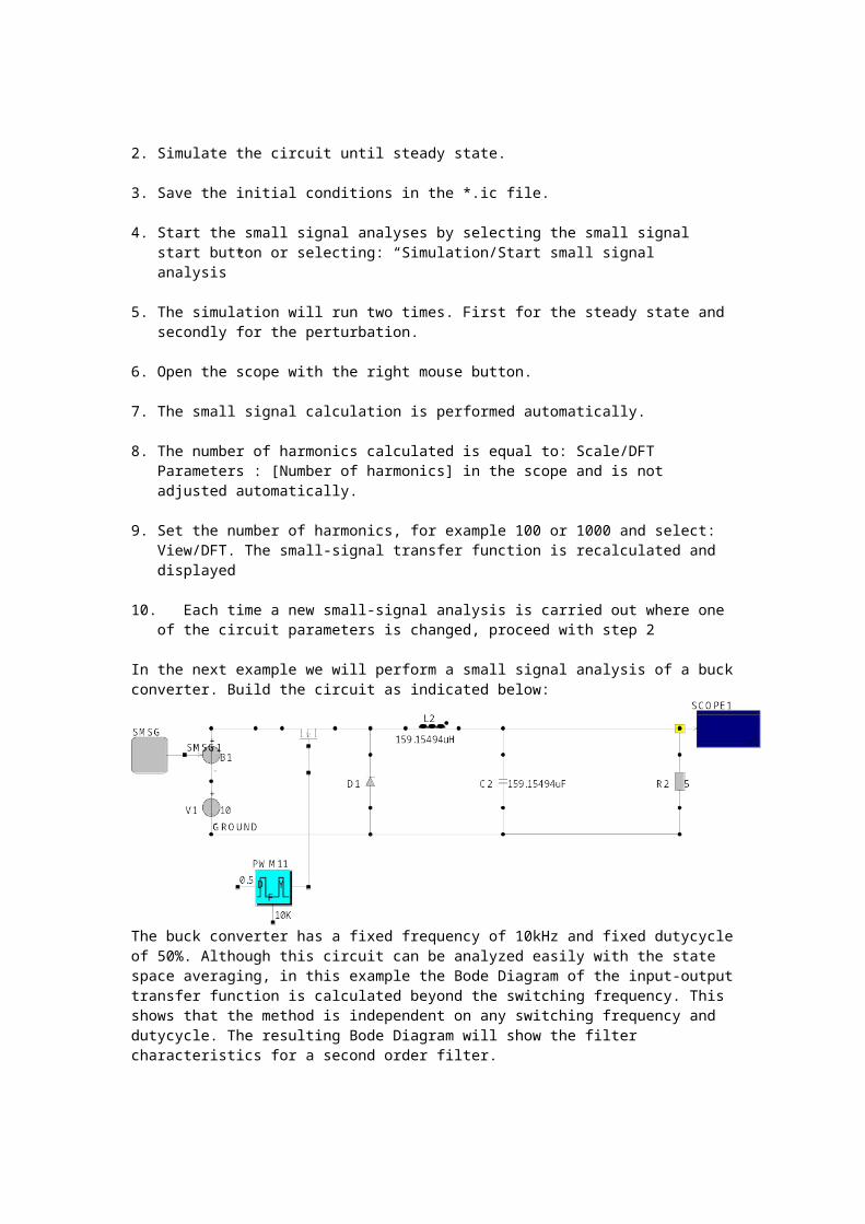
In the next example we will perform a small signal analysis of a buck converter. Build the circuit as indicated below:

The buck converter has a fixed frequency of 10kHz and fixed dutycycle of 50%. Although this circuit can be analyzed easily with the state space averaging, in this example the Bode Diagram of the input-output transfer function is calculated beyond the switching frequency. This shows that the method is independent on any switching frequency and dutycycle. The resulting Bode Diagram will show the filter characteristics for a second order filter.

First simulate the converter until the steady state is reached. Use Tscreen=1ms and dt=1us for the simulation. After reaching the steady state, save the initial condition for this steady state by selecting Tools/Save Initial Condition and save it under the same name as the *.csi file, but with the .ic extension.The parameters for the small signal analysis have to be set in the dialog box “Small signal Parameters”, which can be found in the menu simulation.Select the pulse-width to be equal to the simulation time step dt. In theory the simulation is limited to half the sample frequency so the upper frequency limit is in this case 500kHz. The amplitude of the perturbation is set to 1, which means that the input voltage of 10 volts is perturbed by 10%.

Start the small signala analysis by selecting the menu item “Simulation/Start Small Signal Analysis”

The simulation will start and when finished you can open the scopes by clicking it with the right mouse button. The scope will open and first an analysis is performed. You will see a progress bar in the status bar of the scope.

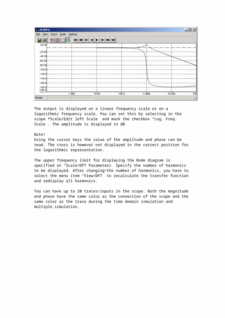
The output is displayed on a linear frequency scale or on a logarithmic frequency scale. You can set this by selecting in the scope “Scale/Edit left Scale” and mark the checkbox “Log. Freq. Scale”. The amplitude is displayed in dB

Note!Using the cursor keys the value of the amplitude and phase can be read. The cross is however not displayed in the correct position for the logarithmic representation.

The upper frequency limit for displaying the Bode diagram is specified at “Scale/DFT Parameters” Specify the number of harmonics to be displayed. After changing the number of harmonics, you have to select the menu item “View/DFT” to recalculate the transfer function and redisplay all harmonics.

You can have up to 20 traces/inputs in the scope. Both the magnitude and phase have the same color as the connection of the scope and the same color as the trace during the time domain simulation and multiple simulation.

Advanced Topic

Coupling to Spice

There is no doubt that Spice is an industry standard for circuit simulation. Therefore there exist a possibility to create simple coupling between Spice and Caspoc. Since Spice simulations tend to be slow and plagued with convergence problems it is not advised create a co simulation between Caspoc and Spice. However Spice can be valuable when one wants to simulate one switching stack in a power converter and thereby using existing spice models for the semiconductors.The following method is advised:A system simulation in Caspoc for a long time period, followed by a spice simulation for only one switching interval.

1Perform a system simulation of the power converter with load and control and thereby using ideal switch models for the semiconductors.Run the simulation until the steady state is achieved. Reset “Tscreen” to one or two switching intervals and continue the simulation for this short period.Store the waveform for the control signals, supply voltages and load current. This is done by displaying each of these waveforms in a scope, and than saving them in ASCII text files by selecting “File / Save” in each Scope.

2Build a Spice model using the detailed semiconductor models and model the control signal, supply voltage and load current by controlled voltage sources, with the value FILE=”caspoc_data_file” instead of a numerical value. Specify the name of the saved text file from the Caspoc-scope instead of caspoc_data_file.Run the simulation in Spice to obtain the waveforms during the switching of the semiconductors.

Advanced Topic.

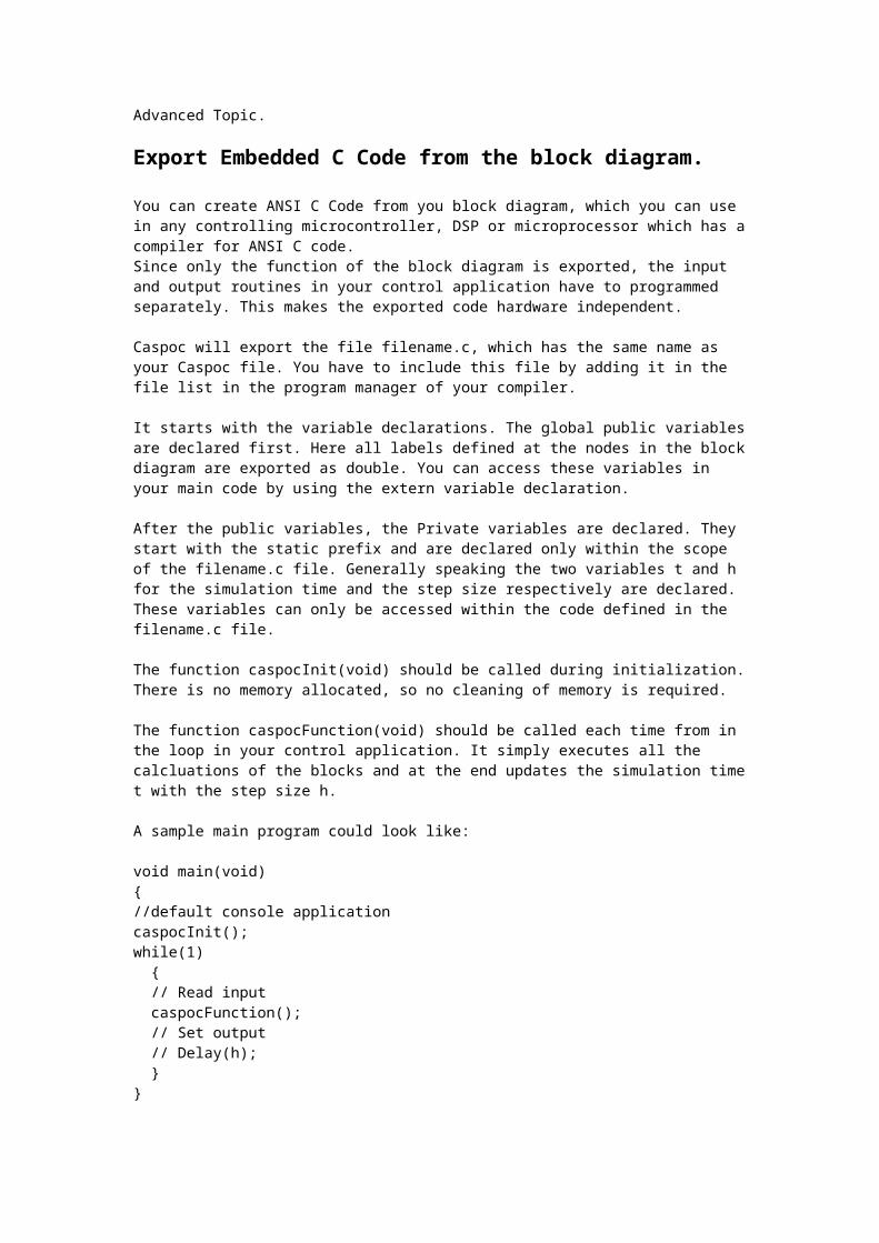
Export Embedded C Code from the block diagram.

You can create ANSI C Code from you block diagram, which you can use in any controlling microcontroller, DSP or microprocessor which has a compiler for ANSI C code.Since only the function of the block diagram is exported, the input and output routines in your control application have to programmed separately. This makes the exported code hardware independent.

Caspoc will export the file filename.c, which has the same name as your Caspoc file. You have to include this file by adding it in the file list in the program manager of your compiler.

It starts with the variable declarations. The global public variables are declared first. Here all labels defined at the nodes in the block diagram are exported as double. You can access these variables in your main code by using the extern variable declaration.

After the public variables, the Private variables are declared. They start with the static prefix and are declared only within the scope of the filename.c file. Generally speaking the two variables t and h for the simulation time and the step size respectively are declared. These variables can only be accessed within the code defined in the filename.c file.

The function caspocInit(void) should be called during initialization. There is no memory allocated, so no cleaning of memory is required.

The function caspocFunction(void) should be called each time from in the loop in your control application. It simply executes all the calcluations of the blocks and at the end updates the simulation time t with the step size h.

A sample main program could look like:

void main(void){//default console applicationcaspocInit();while(1) { // Read input caspocFunction(); // Set output // Delay(h); }}

Advanced Topic

Calculating parasitic inductance in Compare

In Compare you can calculate inductance’s for complicated 3-dimensional wire frames and bus bars. See the user manual for Compare. The calculated inductance’s can be used in the simulation by specifying their value at the component L and the coupling for the component K.

Advanced Topic

Tips and Trick for Spice

“First aid for simulating Power Circuits” by A. Ehle describes some general tips to increase the convergence of Spice and how to model parasitic components in Spice.

“Improving simulation performance of switched mode power supplies” by Bill Pascoe gives more tips and tricks on how to avoid the problems occurring in Spice

“SPICE and SPICE-Iike Simulators have become the de-facto standard simulators for analog and mixed-signal designs. This is true for both Integrated Circuit and board-level designs. Unfortunately, SPICE has not always proven reliable when simulating Switched-Mode Power Supplies (SMPS). Over the past twenty years, numerous solutions at the model level have been put forth to increase the reliability of SMPS simulations. While these solutions do mitigate some of the more egregious problems involved with SMPS simulation, often they add other problems. Recently, simulation and design tools have been introduced that are specifically designed to address the problem of SMPS simulation. In addition, new algorithms have been added to some SPICE Simulators to make the simulation proceed more smoothly. This paper discusses some of the better known model solutions and their limitations, how to increase the reliability of the SPICE simulator with respect to SMPS simulation, and some of the tools that are specifically aimed at design and simulation of SMPS.”

Advanced Topic

Thermal modeling

“Thermal modeling of power electronic systems” by M. März and P. Nance describe how .to use thermal modeling to predict losses in Mosfet models.

The article describes new SPICE and SABER simulation models, which contain a dynamic link between electrical and thermal component descriptions. On the one hand, operating states in which a relevant inherent heating occurs can be simulated under a good approximation of actual conditions. On the other hand, the models offer defined nodes, which provide a link to the thermal environment of the component and enable, for example, the study and optimization of heat sink options.Following a list of the basic properties of the two common thermal equivalent circuit diagrams is a description of the implementation of a dynamic temperature-dependent model in SPICE and SABER using a power MOSFET model as an example. Various possibilities for determining the thermal parameters are demonstrated. The possibilities and limitations of the new models are presented with application-based examples.

Theoretical topic

Numerical Methods

“Everything should be made as simple as possible, but not simpler”- Einstein -

“Een model dat niet werkt is erg. Veel erger echter is een model dat werkt, maar waarvan niemand weet waarom”

- Melvin Asin -

Dit dictaat gaat over de techniek van modelvorming en simulatie. Met de huidige snelle en relatief goedkope computers wordt simulatie van systemen en componenten steeds belangrijker voor de professionele praktijk. De term CASD (Computer Aided System Design) komt steeds vaker voor in de literatuur en illustreert het belang van het onderwerp. Simulatie kan in het bijzonder helpen om inzicht te verkrijgen in het dynamische gedrag van systemen tijdens de ontwerpfase. In het onderwijs wordt simulatie meer en meer gebruikt om de theorie beter te leren begrijpen en vanwege de mogelijkheid voor studenten om zelf de beschreven verschijnselen te onderzoeken.

Simulatie moet worden gedaan met de computer en niet met een theorieboek

Alvorens echter met een pakket kan worden gewerkt, dient de basiskennis van het opzetten, begrenzen en weergeven van een model aanwezig te zijn. Dit dictaat geeft een eerste aanzet in die richting.

INLEIDING IN DEMODELVORMING EN SIMULATIE

VANDYNAMISCHE SYSTEMEN

ir. Willem Dekkers

In Dutch only

Publications

Small signal modeling using time-domain models

Selection of semiconductor models in power electronics simulations

Rapid application development tool Tesla for fast prototyping of electrical machines

Generation of embedded C-code for drive applications

Modeling Electrical Drives

In Dutch only

Appendix

Cscript sample programs

++--

main() {

int i,j; j = 0;

j += 1; j *= 4; j /= 2; j -= 2; j |= 2;

for(i=0;i<10;i+=j-1) print("x");

}

and-or

main() {

test(0,0); test(10,0); test(0,10); test(10,10);}

test(int i, int j) {

puts(""); print(i); print(j); puts("");

if (i && j)

puts("both i and j are non-zero"); else if (i || j) puts("either i and j are non-zero"); else if ((i==0) && (j==0)) puts("both i and j are zero");

}

block

main() { int i; if (i == 1) print("1111111"); else print("0000000");}

break continue

main() {

int i;

puts("loop1: for-break");

for (i=0;i<6;i=i+1) { print("a"); print(i); if (i > 3) break; print("b"); }

puts(""); puts("loop2: for-break in {}");

for (i=0;i<6;i=i+1) {

print("a"); print(i); if (i > 3) { break; } print("b"); }

puts(""); puts("loop3: for-continue");

for (i=0;i<6;i=i+1) { print("a"); print(i); if (i > 3) continue; print("b"); }

puts(""); puts("loop4: while-break");

i = 0; while (i<6) { print("a"); print(i); i=i+1; if (i > 3) break; print("b"); }

puts(""); puts("loop5: while-continue");

i = 0; while (i<6) { print("a"); print(i); i=i+1; if (i > 3) continue; print("b"); }

puts("");

puts("loop6: do-continue");

i = 0; do { print("a"); print(i); i=i+1; if (i > 3) continue; print("b"); } while (i < 6);

puts(""); puts("loop7: do-break");

i = 0; do { print("a"); print(i); i=i+1; if (i > 3) break; print("b"); } while (i < 6);

puts(""); print("ok");}

eob

main() { int i, j; for (i=0;i<3;i=i+1) for(j=0;j<3;j=j+1) print(j+i);

if (i == 1) do {i=i-1;} while(i >-5); i=i-10;// for (i=0;i<10;i=i+1) ;// else

print("0000000");

print(i); puts(""); print("execution ended without problems!");

}

if

main() {

if (1==(1+3)*2-7) print(1); else print(0);

if (1!=(1+3)*2-7) { print(0); } else print(1);

if (1==(1+3)*2-7) print(1); else { print(0); }

if (1!=(1+3)*2-7) { print(0); } else { print(1); }

if (1==1) print("a");

if (1!=1)

print("b");}

loop

main() {

int i;

for (i = 0; i < 2; i = i+1) print(1);

i = 0; for (; i < 2; i = i+1) print(2);

i = 0; for ( ; i < 2; i = i+1) print(3);

for (i = 0;i < 2;) { print(4); i = i + 1; }

for (i = 0; i < 2; ) { print(5); i=i+1; }

print("ok");}

loop2

main() {

int i;

// first test for() and statement on the same line// puts("for() and statement on same line"); for (i = 0; i < 10;i = i+1) print(1); puts("");/* // now with a line break// puts("line-break between for() and statement"); for (i=0;i < 10; i = i+1) print(2); puts("");

// block instead of statement// puts("{ }-block instead of statement"); for (i = 0; i < 10; i = i+1) { print(3); } puts("");

// no initialisation statement in for()// puts("no initialisation statement"); i = 0; for ( ; i < 10; i = i+1) print(4); puts("");*/ for (;;) { print(5); } puts("");

print("ok");}

loop4

main() {

int i;

for (i=0; i<100000; i = i+1) { } print("");}

recursive

main() { recurs(0);}

recurs(int level) {

int i;

i = level+1;

print(i);

if(level == 5) { print("level 5 reached"); }else { recurs(i);} print(i);}

return

main() {

puts("calling function"); test(4); puts("function has returned"); return 0; puts("ERROR - this line comes AFTER main() has returned");}

test(int val) { if (val > 1) { if (val > 2) { if (val > 3) { puts("about to return from function"); return 77; puts("ERROR!"); } } }}

test

int i, j; /* global vars */char ch;

main(){ int i, j;

puts("C Demo Program.");

print_alpha();

do { puts("enter a number (0 to quit): "); i = getnum(); if(i < 0 ) {

puts("numbers must be positive, try again"); } else { for(j = 0; j < i; j=j+1) { print(j); print("summed is"); print(sum(j)); puts(""); } } } while(i!=0);}

/* Sum the values between 0 and num. */sum(int num){ int running_sum;

running_sum = 0;

while(num) { running_sum = running_sum + num; num = num-1; } return running_sum;}

/* Print the alphabet. */print_alpha(){ for(ch = 'A'; ch<='Z'; ch = ch + 1) { putch(ch); } puts("");}