simulation and optimization methods for reliability analysis · simulation and optimization methods...
TRANSCRIPT

Simulation and Optimization Methods forReliability Analysis
M. Oberguggenberger, M. Prackwieser, M. Schwarz
University of Innsbruck, Department of Engineering Science
INTALES GmbH Engineering Solutions
Innsbruck/Natters, Austria
WOST 2013, Weimar, November 21 – 22, 2013
Weimar, November 21, 2013
Oberguggenberger (University of Innsbruck) WOST 2013 Weimar, November 21, 2013 1 / 15

Plan of Presentation
Description of the modelBrute force Monte Carlo benchmarkingQuality assessment of estimators by resampling and Bayes
Cost efficient reliability analysisSubset simulationAsymptotic samplingSensitivity based importance sampling
Optimization and worst case scenariosGenetic algorithmNelder-Mead with constraintsoptiSLang optimization
Structural uncertainties – random field modellingTurning the random field onObserving change of output distribution
Thanks to: Dynardo GmbH, INTALES, CTU Prague, Astrium Ottobrunn
Oberguggenberger (University of Innsbruck) WOST 2013 Weimar, November 21, 2013 2 / 15

Description of the Model
Small launcher model:
FE-model, ABAQUS, 18.000 elements, shellelements and beam elements for stiffeners.91.000 DoF.
35 Input variables x: E-moduli, yield stresses;pressure-, temperature-, booster loads – appliedstepwise; forces due to boundary imperfections.
Input statistics: Uniform distributions with spread±15% around nominal value.
Oberguggenberger (University of Innsbruck) WOST 2013 Weimar, November 21, 2013 3 / 15

Failure Criterion
Output: Failure probability
pf = P(Φ(x) > 1)
defined by the the critical demand-to-capacity ratio (CDCR)
Φ(x) = max
{PEEQ(x)
0.07,SP(x)
180,
0.001
EV (x)
},
combining 3 failure criteria (plastification of metallic part, ruptureof composite part, buckling).
Benchmarking by brute force Monte Carlo, N = 5000, parallelized,performed on the HPC computer LEO III in Innsbruck.
Result of benchmark simulation:
pf = 0.0116.
Oberguggenberger (University of Innsbruck) WOST 2013 Weimar, November 21, 2013 4 / 15

Low Cost Performance Analysis
How good is the Monte Carlo estimator for pf?
First analysis: Bootstrap resampling. Drawing from the originalsample of size N = 5000 with replacement, B = 10000 sampleswith the same (empirical) distribution and corresponding pf areobtained. Result: an estimate of the statistical variation of pf .
Second analysis: Bayesian posterior density for pf , given the dataconstituted by the original sample. The MC-sample can be viewedas the outcome of a Bernoulli experiment (failed/not failed). Theposterior density is an N-fold product of beta distributions.
Variation of pf
around its estimated
value of 0.0116.
Oberguggenberger (University of Innsbruck) WOST 2013 Weimar, November 21, 2013 5 / 15

Reliability Analysis: Faster Methods (1)
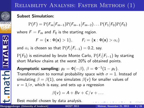
Subset Simulation:
P(F ) = P(Fm∣∣Fm−1)P(Fm−1
∣∣Fm−2) . . .P(F1∣∣F0)P(F0)
where F = Fm and F0 is the starting region.
F = {x : Φ(x) > 1}, Fi = {x : Φ(x) > αi}
and αi is chosen so that P(Fi∣∣Fi−1) = 0.2, say.
P(F0) is estimated by brute Monte Carlo, P(Fi∣∣Fi−1) by starting
short Markov chains at the worst 20% of obtained points.
Asymptotic sampling: pf = Φ(−β), β = Φ−1(1− pf ).Transformation to normal probability space with σ = 1. Instead ofsimulating β = β(1), one simulates β(v) for smaller values ofv = 1/σ, which is easy, and sets up a regression
β(v) = A + Bv + C/v + . . .
Best model chosen by data analysis.
Oberguggenberger (University of Innsbruck) WOST 2013 Weimar, November 21, 2013 6 / 15
Reliability Analysis: Faster Methods (1)
Subset Simulation:
P(F ) = P(Fm∣∣Fm−1)P(Fm−1
∣∣Fm−2) . . .P(F1∣∣F0)P(F0)
where F = Fm and F0 is the starting region.
F = {x : Φ(x) > 1}, Fi = {x : Φ(x) > αi}
and αi is chosen so that P(Fi∣∣Fi−1) = 0.2, say.
P(F0) is estimated by brute Monte Carlo, P(Fi∣∣Fi−1) by starting
short Markov chains at the worst 20% of obtained points.
Asymptotic sampling: pf = Φ(−β), β = Φ−1(1− pf ).Transformation to normal probability space with σ = 1. Instead ofsimulating β = β(1), one simulates β(v) for smaller values ofv = 1/σ, which is easy, and sets up a regression
β(v) = A + Bv + C/v + . . .
Best model chosen by data analysis.Oberguggenberger (University of Innsbruck) WOST 2013 Weimar, November 21, 2013 6 / 15

Reliability Analysis: Faster Methods (2)
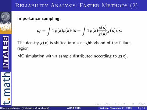
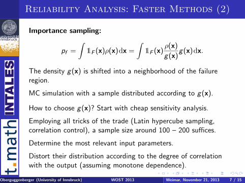
Importance sampling:
pf =
∫1F (x)ρ(x)dx =
∫1F (x)
ρ(x)
g(x)g(x)dx.
The density g(x) is shifted into a neighborhood of the failureregion.
MC simulation with a sample distributed according to g(x).
How to choose g(x)? Start with cheap sensitivity analysis.
Employing all tricks of the trade (Latin hypercube sampling,correlation control), a sample size around 100 – 200 suffices.
Determine the most relevant input parameters.
Distort their distribution according to the degree of correlationwith the output (assuming monotone dependence).
Oberguggenberger (University of Innsbruck) WOST 2013 Weimar, November 21, 2013 7 / 15
Reliability Analysis: Faster Methods (2)
Importance sampling:
pf =
∫1F (x)ρ(x)dx =
∫1F (x)
ρ(x)
g(x)g(x)dx.
The density g(x) is shifted into a neighborhood of the failureregion.
MC simulation with a sample distributed according to g(x).
How to choose g(x)? Start with cheap sensitivity analysis.
Employing all tricks of the trade (Latin hypercube sampling,correlation control), a sample size around 100 – 200 suffices.
Determine the most relevant input parameters.
Distort their distribution according to the degree of correlationwith the output (assuming monotone dependence).
Oberguggenberger (University of Innsbruck) WOST 2013 Weimar, November 21, 2013 7 / 15
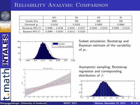
Reliability Analysis: Comparison
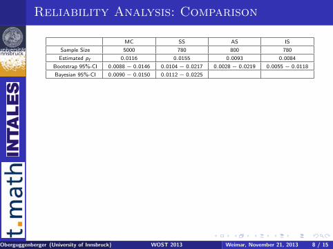
MC SS AS IS
Sample Size 5000 780 800 780
Estimated pf 0.0116 0.0155 0.0093 0.0084
Bootstrap 95%-CI 0.0088 − 0.0146 0.0104 − 0.0217 0.0028 − 0.0219 0.0055 − 0.0118
Bayesian 95%-CI 0.0090 − 0.0150 0.0112 − 0.0225
Subset simulation: Bootstrap andBayesian estimate of the variabilityof pf .
Asymptotic sampling: Bootstrapregression and correspondingdistribution of β.
Oberguggenberger (University of Innsbruck) WOST 2013 Weimar, November 21, 2013 8 / 15
Reliability Analysis: Comparison
MC SS AS IS
Sample Size 5000 780 800 780
Estimated pf 0.0116 0.0155 0.0093 0.0084
Bootstrap 95%-CI 0.0088 − 0.0146 0.0104 − 0.0217 0.0028 − 0.0219 0.0055 − 0.0118
Bayesian 95%-CI 0.0090 − 0.0150 0.0112 − 0.0225
Subset simulation: Bootstrap andBayesian estimate of the variabilityof pf .
Asymptotic sampling: Bootstrapregression and correspondingdistribution of β.
Oberguggenberger (University of Innsbruck) WOST 2013 Weimar, November 21, 2013 8 / 15

Optimization
Derivative-free methods:
Genetic algorithms. An initial set of points is improved (withrespect to the value of the objective function) by randomlychanging coordinates and interchanging components. When alocal optimum has been identified, a restart is undertaken tocover other regions of the search space.
Particle swarms. Similar to genetic algorithms, but the initialset of points is steered towards an optimum by means ofvelocity fields.
Nelder-Mead downhill simplex algorithm. An initial simplex ofpoints is distorted and moved by reflection, expansion,contraction, reduction. Probabilistic restart.
In all cases, the implementation of bounds (on input) andconstraints (on output) requires additional rules.
Oberguggenberger (University of Innsbruck) WOST 2013 Weimar, November 21, 2013 9 / 15
Worst Case Scenarios
First application: In reliability analysis, the location of the failureregion and the most critical points are of interest.
All algorithms compute cloudsof points that can be orderedaccording to their Φ-valuesand used for further analysis.
Subset Simulation (top) andgenetic algorithm (bottom),pressure load sphere 2 versusyield stress cylinder 3.
Legend
yellow 0 − 0.9543
green 0.9544 − 0.9885
blue 0.9886 − 1
red > 1
Oberguggenberger (University of Innsbruck) WOST 2013 Weimar, November 21, 2013 10 / 15
Mass Optimization under Constraint
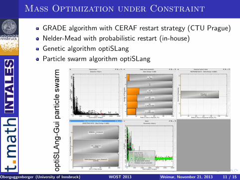
GRADE algorithm with CERAF restart strategy (CTU Prague)
Nelder-Mead with probabilistic restart (in-house)
Genetic algorithm optiSLang
Particle swarm algorithm optiSLang
Oberguggenberger (University of Innsbruck) WOST 2013 Weimar, November 21, 2013 11 / 15
Mass Optimization under Constraint
GRADE algorithm with CERAF restart strategy (CTU Prague)
Nelder-Mead with probabilistic restart (in-house)
Genetic algorithm optiSLang
Particle swarm algorithm optiSLang
Oberguggenberger (University of Innsbruck) WOST 2013 Weimar, November 21, 2013 11 / 15
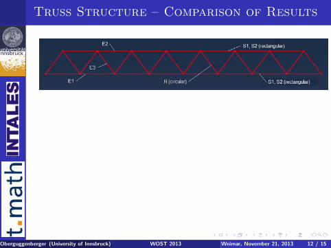
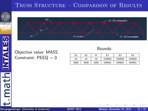
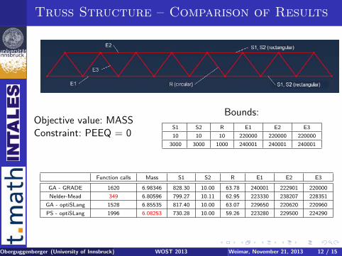
Truss Structure – Comparison of Results
Objective value: MASSConstraint: PEEQ = 0
Bounds:
S1 S2 R E1 E2 E3
10 10 10 220000 220000 220000
3000 3000 1000 240001 240001 240001
Function calls Mass S1 S2 R E1 E2 E3
GA - GRADE 1620 6.98346 828.30 10.00 63.78 240001 222901 220000
Nelder-Mead 349 6.80596 799.27 10.11 62.95 223330 238207 228351
GA - optiSLang 1528 6.85535 817.40 10.00 63.07 229650 220620 220960
PS - optiSLang 1996 6.08253 730.28 10.00 59.26 223280 229500 224290
Oberguggenberger (University of Innsbruck) WOST 2013 Weimar, November 21, 2013 12 / 15

Random Field Modelling (1)
A random field on the small launcher model (material properties)
Determination of field parameters from empirical dataspectral decomposition of covariance matrixMonte Carlo simulation of the random field (Karhunen-Loeve)repeated FE-calculation of structural response
Typical autocovariance function
COV(XP ,XQ) = σ2 exp(−dist1(P,Q)/`1) exp(−dist2(P,Q)/`2)
Oberguggenberger (University of Innsbruck) WOST 2013 Weimar, November 21, 2013 13 / 15

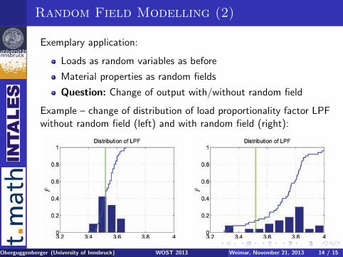
Random Field Modelling (2)
Exemplary application:
Loads as random variables as before
Material properties as random fields
Question: Change of output with/without random field
Example – change of distribution of load proportionality factor LPFwithout random field (left) and with random field (right):
Oberguggenberger (University of Innsbruck) WOST 2013 Weimar, November 21, 2013 14 / 15

Thank you for your attention!