• Simulation-Based Estimation of Continuous Time Models in R

• R/Finance 2010

• Eric Zivot• University of Washington

• Joint work with:

• Peter Fuleky• University of Hawaii

© Eric Zivot 2010

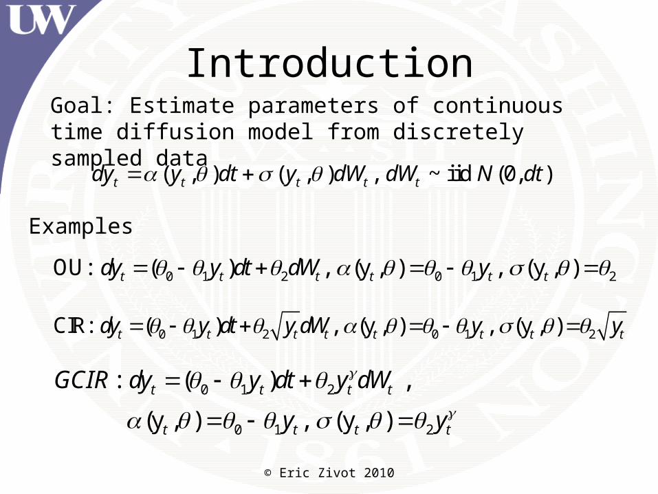
IntroductionGoal: Estimate parameters of continuous time diffusion model from discretely sampled data

( , ) ( , ) , ~ iid (0, )t t t t tdy y dt y dW dW N dt

Examples

0 1 2 0 1 2OU: ( ) , (y , ) , (y , )t t t t t tdy y dt dW y

0 1 2 0 1 2CIR: ( ) , (y , ) , (y , )t t t t t t t tdy y dt y dW y y

0 1 2

0 1 2

: ( ) ,

(y , ) , (y , )

t t t t

t t t t

GCIR dy y dt y dW

y y

© Eric Zivot 2010

Estimation Methods

• MLE – often not feasible• MLE of approximated model – difficult• QMLE of discretized model – easy but biased• GMM – inefficient and biased• Bayesian MCMC Methods - promising • Indirect Inference – Corrects bias in QMLE– focus of talk

© Eric Zivot 2010

Indirect Inference

• Distance-based methodology (aka II) developed by Smith (1993), Gourierioux, Monfort, and Renault (1993)

• Score-based methodology (aka EMM) developed by Gallant and Tauchen (1996)

II EMM

II

EMM

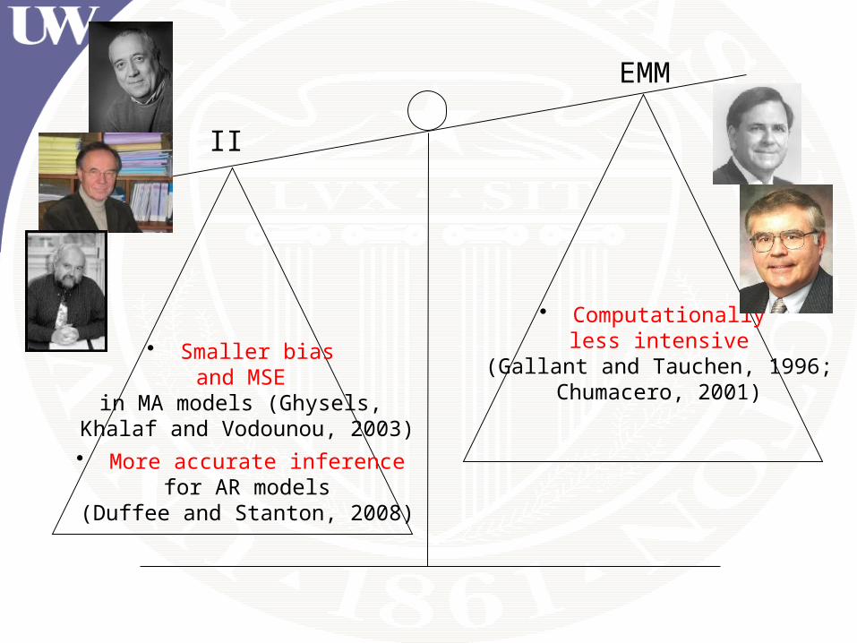
• Computationally less intensive

(Gallant and Tauchen, 1996;Chumacero, 2001)

II EMM

• Smaller bias and MSE

in MA models (Ghysels, Khalaf and Vodounou, 2003)

• Computationally less intensive

(Gallant and Tauchen, 1996;Chumacero, 2001)

II

EMM

• Smaller bias and MSE

in MA models (Ghysels, Khalaf and Vodounou, 2003)• More accurate inference

for AR models(Duffee and Stanton, 2008)

• Computationally less intensive

(Gallant and Tauchen, 1996;Chumacero, 2001)

© Eric Zivot 2010

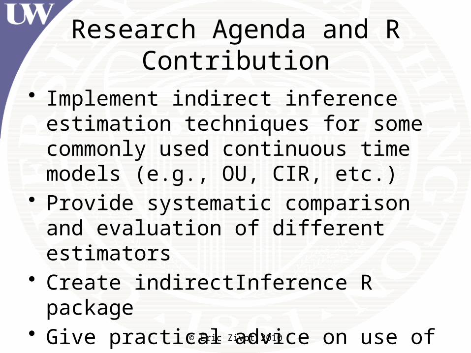
Research Agenda and R Contribution

• Implement indirect inference estimation techniques for some commonly used continuous time models (e.g., OU, CIR, etc.)

• Provide systematic comparison and evaluation of different estimators

• Create indirectInference R package• Give practical advice on use of techniques

Indirect Inference Set-up

( 1)

arg max { } , , where

1( ; , ), { }

nn t t

nt

n t t t i i t mt m

Q y

Q f y x x yn m

{ } observations with observation interval nt ty

Structural model: , , stationary and ergodicpF

Auxiliary model: , , rF r p

( ; , ) conditional log density of for the model t t tf y x y F

( ) arg max [ ( ; , )] lim under

binding function

F t tE f y x p F

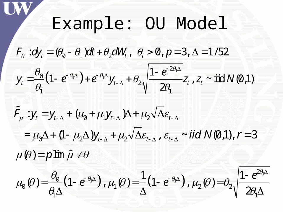
Example: OU Model

1

1 1

0 1 2

20

21 1

: ( ) , 0, 3, 1/ 52

11 , ~ iid (0,1)

2

t t i

t t t t

F dy dt dW p

ey e e y z z N

0 1 2

0 2 2

: ( )

= (1 ) , ~ (0,1), 3

t t t t

t t t

F y y y

y iid N r

1

1 1

20

0 1 2 21 1

( ) lim

1 1( ) 1 , ( ) 1 , ( )

2

p

ee e

© Eric Zivot 2010

Example: OU Model• Estimating the “crude Euler” auxiliary model

leads to biased estimates (Lo, 1988)– Asymptotic discretization bias = μ(θ) – θ – μ(θ) – θ → 0 as Δ → 0

• μ(θ) is invertible giving analytic II estimates

1

1

00 1 1 1

1

12 2 ln(1 )

ˆ ( )

1ˆ ˆln(1 ), ln(1 ),

2 ln(1 )ˆ1

II

II II

II

e

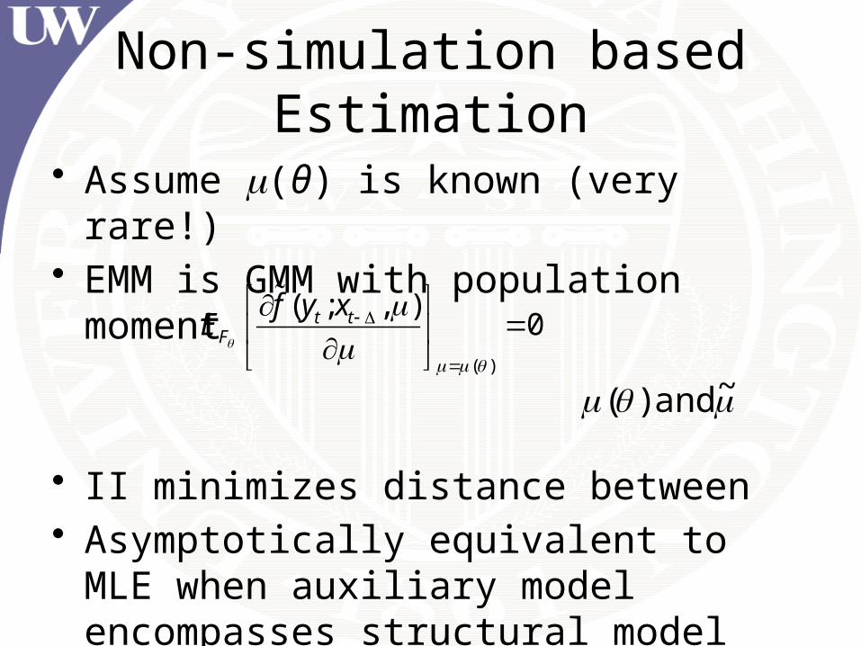
Non-simulation based Estimation

• Assume m(θ) is known (very rare!)• EMM is GMM with population moment

• II minimizes distance between• Asymptotically equivalent to MLE when

auxiliary model encompasses structural model

( )

( ; , )0t t

F

f y xE

~ and )(

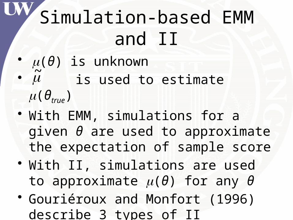
Simulation-based EMM and II

• m(θ) is unknown• is used to estimate m(θtrue)

• With EMM, simulations for a given θ are used to approximate the expectation of sample score

• With II, simulations are used to approximate m(θ) for any θ

• Gouriéroux and Monfort (1996) describe 3 types of II estimators and 2 types of EMM estimators

~

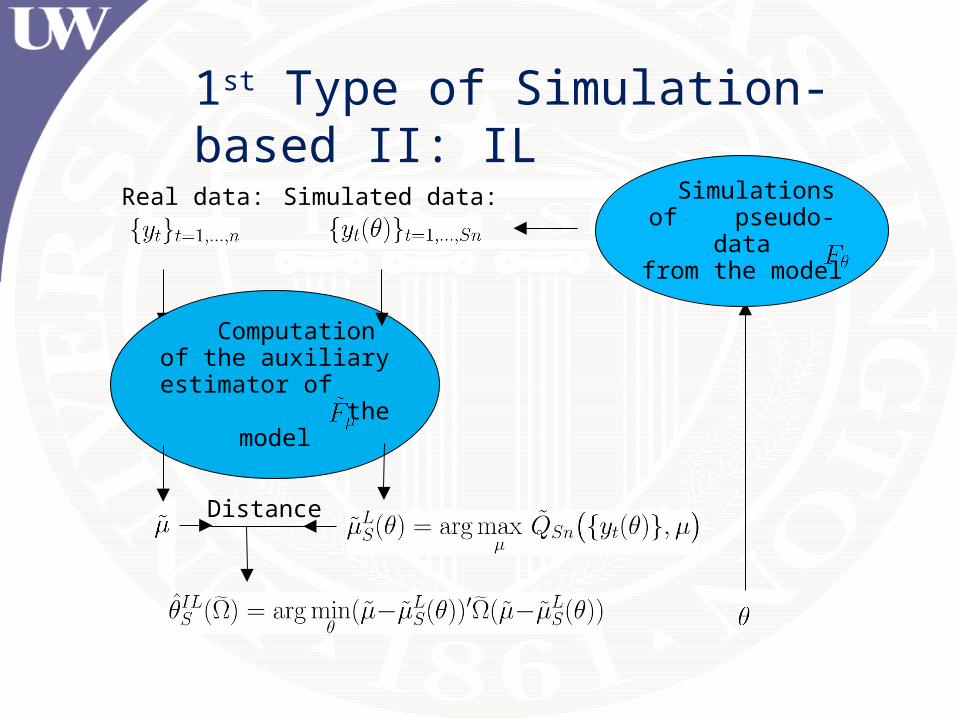
Distance

Computation of the auxiliary estimator of

the model

Simulations of pseudo-data

from the model

Real data: Simulated data:

1st Type of Simulation-based II: IL

Distance

Computation of the auxiliary estimator of

the model

Simulations of pseudo-data

from the model

Real data: Simulated data:

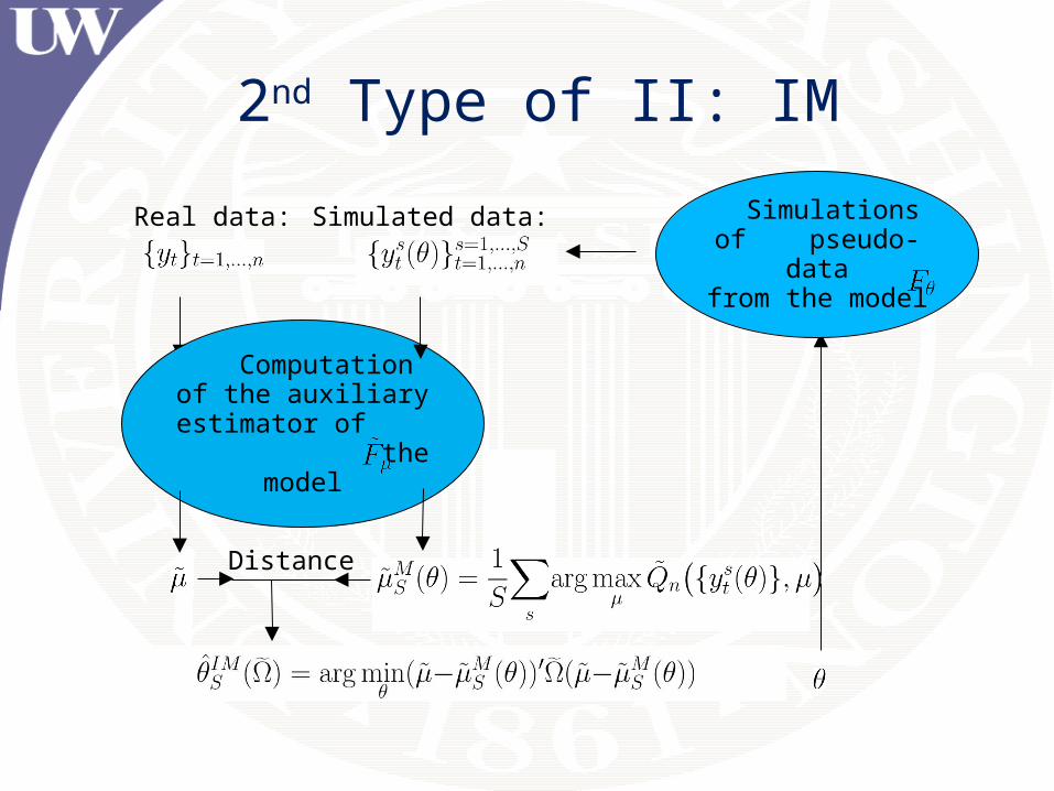
2nd Type of II: IM

Distance

Computation of the auxiliary estimator of

the model

Simulations of pseudo-data

from the model

Real data: Simulated data:

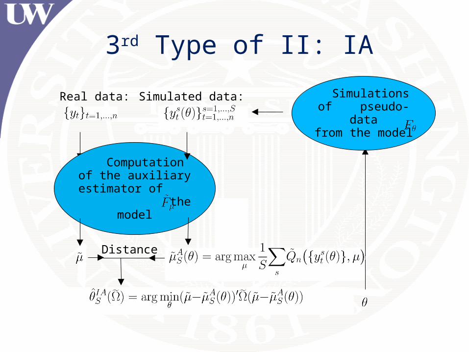
3rd Type of II: IA

Distance

Computation of the auxiliary estimator and

score of the model

Simulations of pseudo-data

from the model

Real data: Simulated data:

1st Type of EMM: EL

Distance

Computation of the auxiliary estimator and

score of the model

Simulations of pseudo-data

from the model

Real data: Simulated data:

2nd Type of EMM: EA

© Eric Zivot 2010

R Implementation of II• Estimate Euler auxiliary model parameters μ

from observed data {yt} by QMLE

– Use function EULERloglik() from R package sde

– Use R function optim()

( , ) ( , ) , z ~ iid (0,1)t t t t t ty y y y z N

( 1)

arg max { } , , where

1( ; , ), { }

nn t t

nt

n t t t i i t mt m

Q y

Q f y x x yn m

© Eric Zivot 2010

R Implementation of II

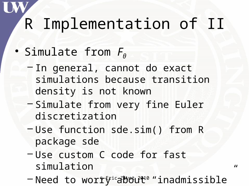
• Simulate from Fθ – In general, cannot do exact simulations because

transition density is not known– Simulate from very fine Euler discretization– Use function sde.sim() from R package sde– Use custom C code for fast simulation– Need to worry about “inadmissible” or

“explosive” simulations from inappropriate θ – need to “bullet proof” the simulator

© Eric Zivot 2010

R Implementation of II

• For distance-based II, estimate binding function μ(θ) from simulated data

– Use same random number seed for all θ

{ ( )}sty

( 1)

arg max { ( )}, , where

1( ( ); ( ), ),

L sS Sn t

Sns s

Sn t tt m

Q y

Q f y xn

© Eric Zivot 2010

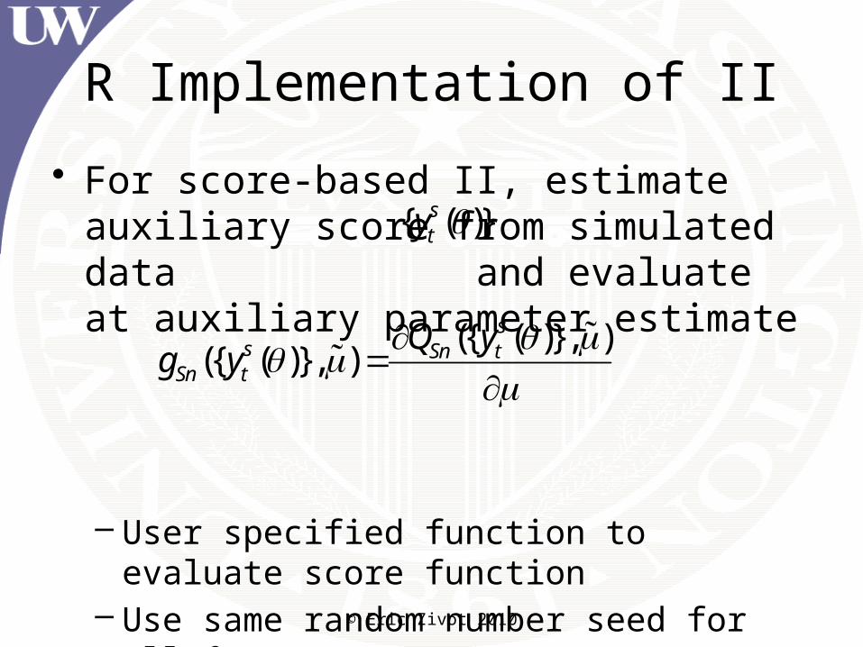
R Implementation of II

• For score-based II, estimate auxiliary score from simulated data and evaluate at auxiliary parameter estimate

– User specified function to evaluate score function– Use same random number seed for all θ

({ ( )}, )({ ( )}, )

ss Sn t

Sn t

Q yg y

{ ( )}sty

© Eric Zivot 2010

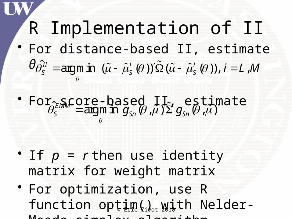
R Implementation of II• For distance-based II, estimate θ

• For score-based II, estimate

• If p = r then use identity matrix for weight matrix

• For optimization, use R function optim() with Nelder-Meade simplex algorithm

ˆ arg min ( ( )) ( ( )), ,II i iS S S i L M

ˆ arg min ( , ) ( , )EMMS Sn Sng g

© Eric Zivot 2010

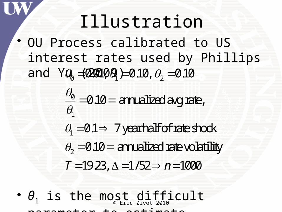
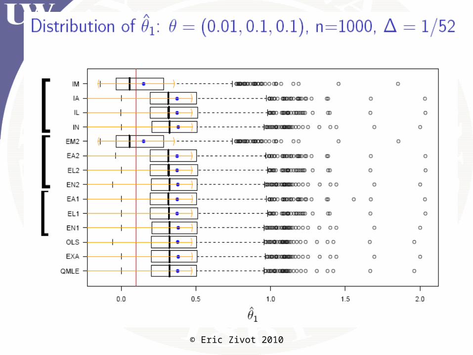
Illustration• OU Process calibrated to US interest rates

used by Phillips and Yu (2009)

• θ1 is the most difficult parameter to estimate

0 1 2

0

1

1

2

0.01, 0.10, 0.10

0.10 annualized avg rate,

0.1 7 year half of rate shock

0.10 annualized rate volatility

19.23, 1/ 52 1000T n

© Eric Zivot 2010

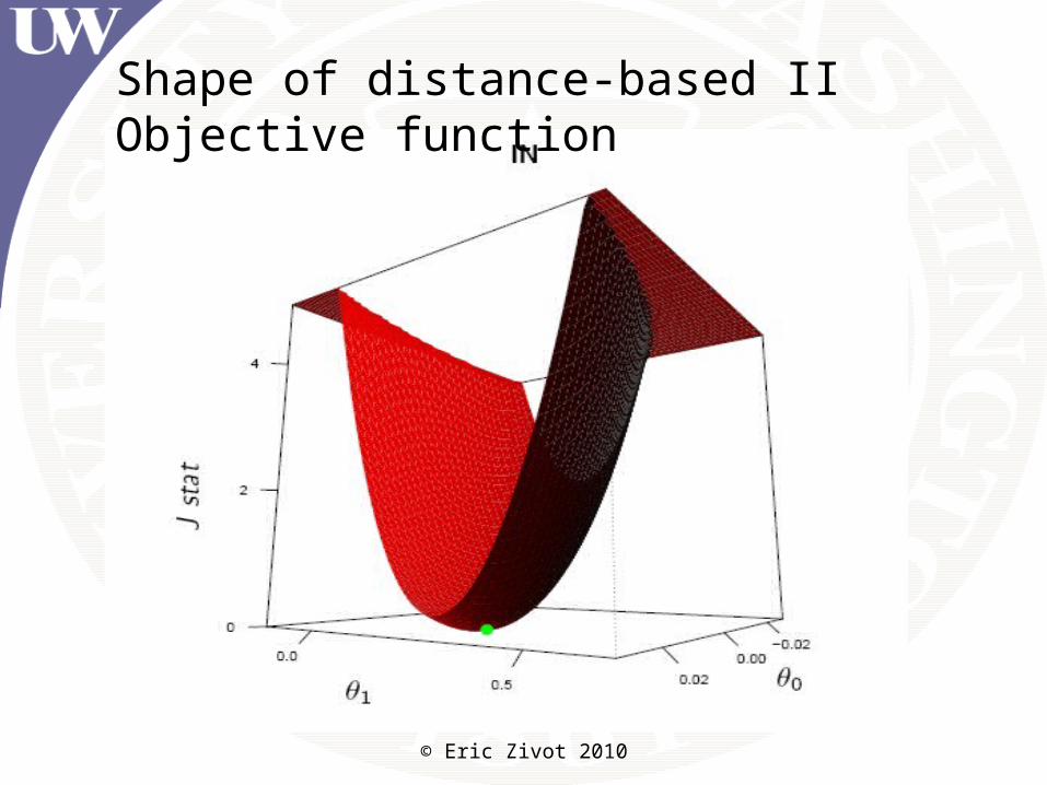
Shape of distance-based II Objective function

© Eric Zivot 2010

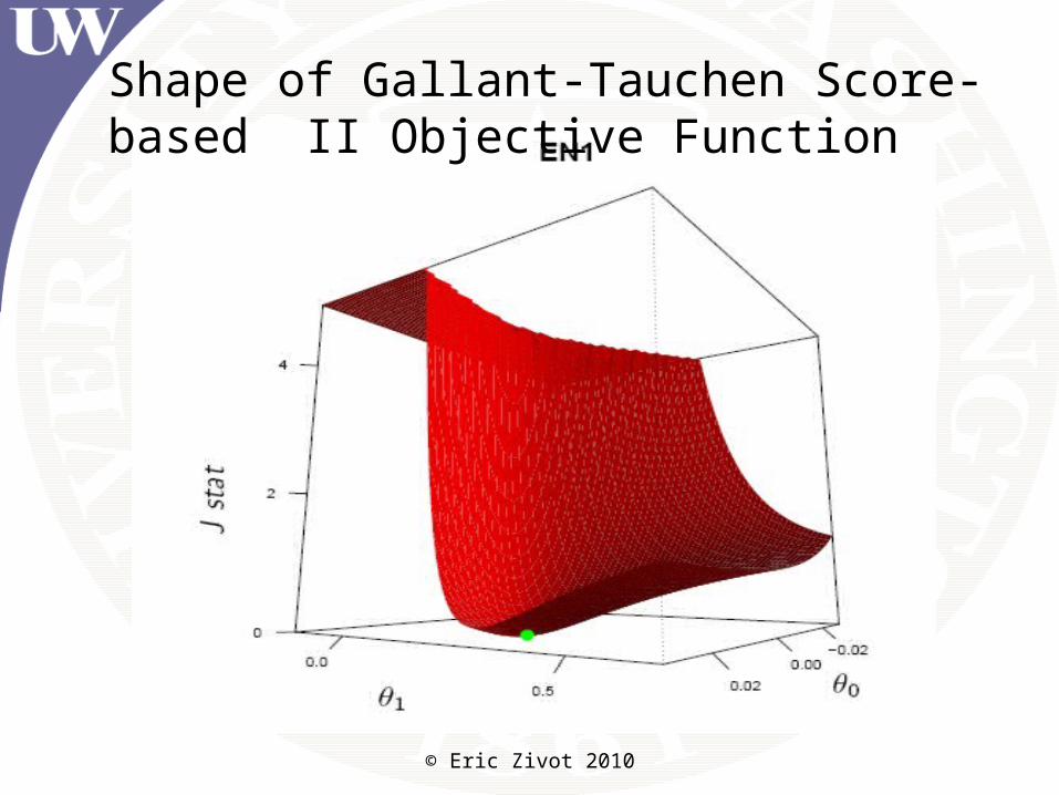
Shape of Gallant-Tauchen Score-based II Objective Function

© Eric Zivot 2010

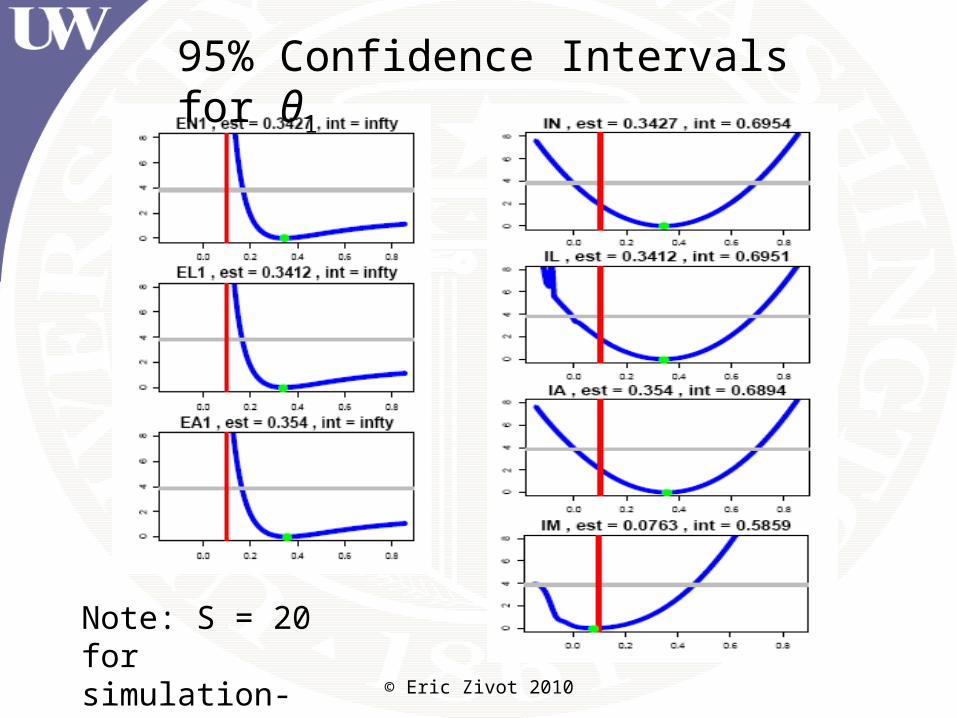
95% Confidence Intervals for θ1

Note: S = 20 for simulation-based estimates

© Eric Zivot 2010

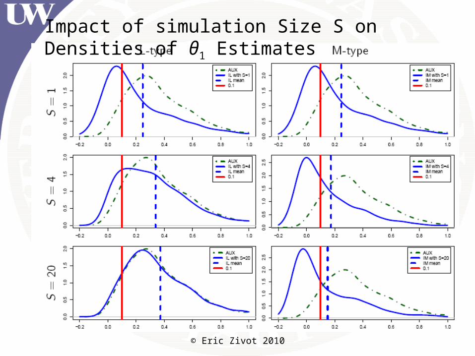
Impact of simulation Size S on Densities of θ1 Estimates

© Eric Zivot 2010

© Eric Zivot 2010

© Eric Zivot 2010

© Eric Zivot 2010

© Eric Zivot 2010

Research in Progress

• Fuleky, P., and Zivot, E. (2010). Further Evidence on Simulation Inference for Near Unit Root Processes with Implications for Term Structure Estimation. Manuscript in preparation.

• Fuleky, P., and Zivot, E. (2010). Indirect Inference Based on the Score. Manuscript in preparation.

• Fuleky, P., and Zivot, E. (2010). indirectInference: R package for indirect inference.

© Eric Zivot 2010

References

• Duffee, G. and Stanton, R. (2008). Evidence on Simulation Inference for Near Unit-Root Processes with Implications for Term Structure Estimation. Journal of Financial Econometrics, 6(1):108.

• Gallant, A. and Tauchen, G. (1996). Which Moments to Match? Econometric Theory, 12(4):657-81.

• Lo, A. (1988). Maximum Likelihood Estimation of Generalized Ito Processes with Discretely Sampled Data. Econometric Theory, 4(2):231-247.

• Gourieroux, C. and Monfort, A. (1996). Simulation-Based Econometric Methods. Oxford University Press, USA.

© Eric Zivot 2010

References

• Gourieroux, C., Monfort, A., and Renault, E. (1993). Indirect Inference. Journal of Applied Econometrics, 8:S85-S118.

• Phillips, P. and Yu, J. (2009). Maximum Likelihood and Gaussian Estimation of Continuous Time Models in Finance. Handbook of Financial Time Series.

• Smith Jr, A. (1993). Estimating Nonlinear Time-Series Models Using Simulated Vector Autoregressions. Journal of Applied Econometrics, 8:S63-S84.