simulation-based optimization for production planning
TRANSCRIPT
Simulation-Based Optimization for Production Planning:
Integrating Meta-Heuristics, Simulation and Exact Techniques to
Address the Uncertainty and Complexity of Manufacturing Systems
A thesis submitted to the University of Manchester
for the degree of Doctor of Philosophy
in the Faculty of Humanities
2016
Juan Esteban Diaz Leiva
Alliance Manchester Business School
Contents
List of Abbreviations 13
Abstract 16
Declaration 17
Copyright 18
Dedication 20
Acknowledgements 21
1 Introduction 22
1.1 Research Context . . . . . . . . . . . . . . . . . . . . . . . . . . . . 22
1.2 Research Aim . . . . . . . . . . . . . . . . . . . . . . . . . . . . . . 24
1.3 Contributions of the Thesis . . . . . . . . . . . . . . . . . . . . . . . 25
1.4 Structure of the Thesis . . . . . . . . . . . . . . . . . . . . . . . . . 26
1.5 Publications Resulting from the Thesis . . . . . . . . . . . . . . . . . 28
2 Description of the Manufacturing System Analysed 30
2.1 Batch Manufacturing System . . . . . . . . . . . . . . . . . . . . . . 31
2.2 Production Planning Challenges . . . . . . . . . . . . . . . . . . . . 41
2.3 Production Planning Problem . . . . . . . . . . . . . . . . . . . . . . 42
2
3 Initial Simulation-Based Optimization Model (Manuscript 1) 44
3.1 Abstract . . . . . . . . . . . . . . . . . . . . . . . . . . . . . . . . . 44
3.2 Introduction . . . . . . . . . . . . . . . . . . . . . . . . . . . . . . . 45
3.3 Simulation-based Optimization Model . . . . . . . . . . . . . . . . . 48
3.3.1 Simulation Model . . . . . . . . . . . . . . . . . . . . . . . 49
3.3.2 Optimization Model . . . . . . . . . . . . . . . . . . . . . . 53
3.4 Preliminary Results . . . . . . . . . . . . . . . . . . . . . . . . . . . 55
3.5 Future Research . . . . . . . . . . . . . . . . . . . . . . . . . . . . . 56
4 Noise Handling Strategies (Manuscript 2) 59
4.1 Abstract . . . . . . . . . . . . . . . . . . . . . . . . . . . . . . . . . 59
4.2 Introduction . . . . . . . . . . . . . . . . . . . . . . . . . . . . . . . 60
4.3 Simulation-Based Optimization Model . . . . . . . . . . . . . . . . . 63
4.3.1 Simulation Model . . . . . . . . . . . . . . . . . . . . . . . 64
4.3.2 Optimization Model . . . . . . . . . . . . . . . . . . . . . . 65
4.4 Noise Handling Strategies . . . . . . . . . . . . . . . . . . . . . . . 66
4.5 Comparative Analysis . . . . . . . . . . . . . . . . . . . . . . . . . . 68
4.6 Results . . . . . . . . . . . . . . . . . . . . . . . . . . . . . . . . . . 70
4.7 Conclusion . . . . . . . . . . . . . . . . . . . . . . . . . . . . . . . 74
4.8 Limitations and Future Research . . . . . . . . . . . . . . . . . . . . 75
5 Integrating Meta-Heuristics and Exact Optimization Techniques (Manuscript
3) 77
5.1 Abstract . . . . . . . . . . . . . . . . . . . . . . . . . . . . . . . . . 77
5.2 Introduction . . . . . . . . . . . . . . . . . . . . . . . . . . . . . . . 78
5.3 Literature Review . . . . . . . . . . . . . . . . . . . . . . . . . . . . 80
5.3.1 Simulation-based optimization . . . . . . . . . . . . . . . . . 82
5.3.2 Contributions . . . . . . . . . . . . . . . . . . . . . . . . . . 86
3
5.4 Problem Description . . . . . . . . . . . . . . . . . . . . . . . . . . 87
5.4.1 New Variants of the KP Problem: d-MBKAR and d-MBKARS 89
5.5 Simulation-Based Optimization Model . . . . . . . . . . . . . . . . . 93
5.5.1 Optimization Model . . . . . . . . . . . . . . . . . . . . . . 96
5.5.2 Initialization Operators . . . . . . . . . . . . . . . . . . . . . 97
5.5.3 Repair Operator . . . . . . . . . . . . . . . . . . . . . . . . . 101
5.6 Benchmark Analysis . . . . . . . . . . . . . . . . . . . . . . . . . . 101
5.6.1 Results . . . . . . . . . . . . . . . . . . . . . . . . . . . . . 103
5.7 Conclusion . . . . . . . . . . . . . . . . . . . . . . . . . . . . . . . 108
5.8 Limitations and Future Research . . . . . . . . . . . . . . . . . . . . 109
6 A Matheuristic Optimizer to Address the d-MBKARS Problem 115
6.1 Abstract . . . . . . . . . . . . . . . . . . . . . . . . . . . . . . . . . 115
6.2 Introduction . . . . . . . . . . . . . . . . . . . . . . . . . . . . . . . 116
6.3 SBOMat Approach . . . . . . . . . . . . . . . . . . . . . . . . . . . 118
6.4 Benchmark Analysis . . . . . . . . . . . . . . . . . . . . . . . . . . 120
6.5 Results . . . . . . . . . . . . . . . . . . . . . . . . . . . . . . . . . . 120
6.6 Conclusion . . . . . . . . . . . . . . . . . . . . . . . . . . . . . . . 121
7 Simulating Realistic Features of Manufacturing Systems 125
7.1 New Extensions . . . . . . . . . . . . . . . . . . . . . . . . . . . . . 126
7.2 Conclusion . . . . . . . . . . . . . . . . . . . . . . . . . . . . . . . 135
8 Evolutionary Robust Optimization (Manuscript 4) 136
8.1 Abstract . . . . . . . . . . . . . . . . . . . . . . . . . . . . . . . . . 136
8.2 Introduction . . . . . . . . . . . . . . . . . . . . . . . . . . . . . . . 137
8.2.1 Robust Optimization . . . . . . . . . . . . . . . . . . . . . . 139
8.2.2 Evolutionary Robust Optimization . . . . . . . . . . . . . . . 140
4
8.2.3 Contributions . . . . . . . . . . . . . . . . . . . . . . . . . . 142
8.3 Simulation-Based Optimization Model . . . . . . . . . . . . . . . . . 144
8.3.1 Optimization Model . . . . . . . . . . . . . . . . . . . . . . 145
8.3.2 Initialization Operator . . . . . . . . . . . . . . . . . . . . . 150
8.4 Benchmark Analysis . . . . . . . . . . . . . . . . . . . . . . . . . . 152
8.5 Performance Assessment . . . . . . . . . . . . . . . . . . . . . . . . 155
8.6 Results . . . . . . . . . . . . . . . . . . . . . . . . . . . . . . . . . . 157
8.7 Conclusion . . . . . . . . . . . . . . . . . . . . . . . . . . . . . . . 167
9 Conclusion 180
Word Count: 47558
5
List of Tables
2.1 Products manufactured in the different production lines. . . . . . . . . 32
2.2 Requirements of products manufactured in the system that are used as
raw materials. . . . . . . . . . . . . . . . . . . . . . . . . . . . . . . 33
2.3 Product lot characteristics and demand level. . . . . . . . . . . . . . . 36
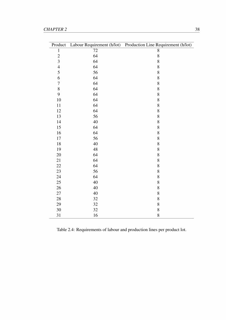
2.4 Requirements of labour and production lines per product lot. . . . . . 38
2.5 Conservative probabilities of failure and average detention time per
production line. . . . . . . . . . . . . . . . . . . . . . . . . . . . . . 40
3.1 Number of product lots to be manufactured in a specific production line. 57
3.2 Demand, consolidated production plan per product and actual produc-
tion achieved. . . . . . . . . . . . . . . . . . . . . . . . . . . . . . . 58
4.1 Parameters used for baseline, implicit averaging, explicit averaging
and hybrid strategies. . . . . . . . . . . . . . . . . . . . . . . . . . . 68
4.2 pl per problem instance and PDFs specifications to model Λl . . . . . . 69
4.3 Descriptive statistics of average profits and average computation times
per strategy in problem instance 1. . . . . . . . . . . . . . . . . . . . 71
4.4 Descriptive statistics of average profits and average computation times
per strategy in problem instance 2. . . . . . . . . . . . . . . . . . . . 71
4.5 Values for Mann-Whitney U statistic obtained in problem instance 1. . 72
4.6 Values for Mann-Whitney U statistic obtained in problem instance 2. . 72
6
5.1 pl per problem instance and PDFs specifications to model Λl . . . . . . 103
5.2 Computational time in seconds for each model per problem instance. . 106
5.3 Possible parameter values given to irace. . . . . . . . . . . . . . . . 110
5.4 Values for Mann-Whitney U statistic obtained for average profit values. 111
5.5 Sample mean and sample standard deviation of the average profit val-
ues returned by the best ILP-derived solutions and by the final solu-
tions obtained with SBO1 and SBO2 across 30 runs. . . . . . . . . . 114
6.1 Values for Mann-Whitney U statistic obtained for average profit values. 124
7.1 Transition probability matrix. . . . . . . . . . . . . . . . . . . . . . . 130
8.1 Values of pl , µl,T , ζl and ϕl per production line and problem instance. 154
8.2 Objective/s, γ and number of generations across the different models
analysed. . . . . . . . . . . . . . . . . . . . . . . . . . . . . . . . . 155
8.3 Values for Mann-Whitney U statistic obtained from pairwise compar-
isons of hypervolume values of all single and multi-objective models
in the objective space of average profit vs. standard deviation of profit
in problem instance 1. . . . . . . . . . . . . . . . . . . . . . . . . . . 165
8.4 Values for Mann-Whitney U statistic obtained from pairwise compar-
isons of hypervolume values of all single and multi-objective models
in the objective space of average profit vs. minimum profit in problem
instance 1. . . . . . . . . . . . . . . . . . . . . . . . . . . . . . . . . 166
8.5 Values for Mann-Whitney U statistic obtained from pairwise compar-
isons of hypervolume values of all single and multi-objective models
in the objective space of average profit vs. standard deviation of profit
in problem instance 2. . . . . . . . . . . . . . . . . . . . . . . . . . . 178
7

8.6 Values for Mann-Whitney U statistic obtained from pairwise compar-
isons of hypervolume values of all single and multi-objective models
in the objective space of average profit vs. minimum profit in problem
instance 2. . . . . . . . . . . . . . . . . . . . . . . . . . . . . . . . . 179
8
List of Figures
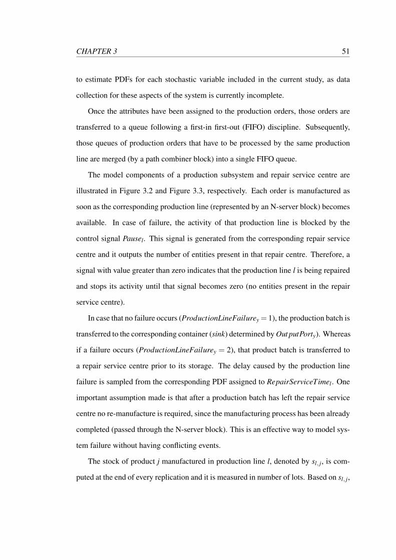
3.1 Order processing subsystem for production line l. . . . . . . . . . . . 50
3.2 Production subsystem for production line l. . . . . . . . . . . . . . . 52
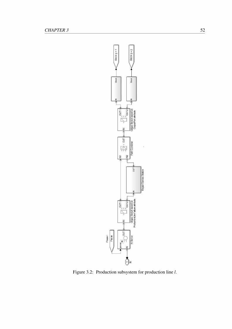
3.3 Repair service centre of production line l. . . . . . . . . . . . . . . . 53
3.4 Best, mean and worst fitness value of the population at each iteration. 56
4.1 CDFs of average profit values obtained with production plans gener-
ated under the four different strategies in problem instance 1. . . . . . 73
4.2 CDFs of average profit values obtained with production plans gener-
ated under the four different strategies in problem instance 2. . . . . . 74
5.1 SBO model. . . . . . . . . . . . . . . . . . . . . . . . . . . . . . . . 94
5.2 CDFs of average profit values generated with solutions given by SBO1,
SBO2, SBO3, CCP and ILP in problem instance 1 (low uncertainty). . 106
5.3 CDFs of average profit values generated with solutions given by SBO1,
SBO2, SBO3, CCP and ILP in problem instance 2 (medium uncertainty).107
5.4 CDFs of average profit values generated with solutions given by SBO1,
SBO2, SBO3, CCP and ILP in problem instance 3 (high uncertainty). 107
5.5 CDFs of average profit values generated with solutions given by SBO1,
SBO2, SBO3 and SBO3x2 in problem instance 1 (low uncertainty). . 112
5.6 CDFs of average profit values generated with solutions given by SBO1,
SBO2, SBO3 and SBO3x2 in problem instance 2 (medium uncertainty). 112
9
5.7 CDFs of average profit values generated with solutions given by SBO1,
SBO2, SBO3 and SBO3x2 in problem instance 3 (high uncertainty). . 113
6.1 SBOMat approach. . . . . . . . . . . . . . . . . . . . . . . . . . . . 119
6.2 CDFs of average profit values generated with solutions given by SBO1,
SBO2 and SBOMat in problem instance 1 (low uncertainty). . . . . . 122
6.3 CDFs of average profit values generated with solutions given by SBO1,
SBO2 and SBOMat in problem instance 2 (medium uncertainty). . . . 122
6.4 CDFs of average profit values generated with solutions given by SBO1,
SBO2 and SBOMat in problem instance 3 (high uncertainty). . . . . . 123
7.1 Order initialization sub-system of production line 2. . . . . . . . . . . 127
7.2 Final product sub-system of production line 2. . . . . . . . . . . . . . 128
7.3 Manufacturing sub-system of production line 2. . . . . . . . . . . . . 129
7.4 Markov chain. . . . . . . . . . . . . . . . . . . . . . . . . . . . . . . 131
7.5 Repair sub-system of production line 2. . . . . . . . . . . . . . . . . 134
8.1 CDFs of hypervolume values obtained with multi-objective models
(MSBO-1A, MSBO-2A, MSBO-1B, MSBO-2B) in the objective space
of average profit vs. standard deviation of profit in problem instance 1. 158
8.2 CDFs of hypervolume values obtained with multi-objective models
(MSBO-1A, MSBO-2A, MSBO-1B, MSBO-2B) in the objective space
of average profit vs. minimum profit in problem instance 1. . . . . . . 159
8.3 CDFs of hypervolume values obtained with the best multi-objective
model (MSBO-1B) and all single-objective models (SSBO-1A, SSBO-
2A, SSBO-1B and SSBO-2B) in the objective space of average profit
vs. standard deviation of profit. . . . . . . . . . . . . . . . . . . . . . 160
10
8.4 CDFs of hypervolume values obtained with the best multi-objective
model (MSBO-1B) and all single-objective models (SSBO-1A, SSBO-
2A, SSBO-1B and SSBO-2B) in the objective space of average profit
vs. minimum profit. . . . . . . . . . . . . . . . . . . . . . . . . . . . 161
8.5 Median (dashed line) and best (continuous line) attainment surfaces of
the best multi-objective model and all single-objective models in the
objective space of average profit vs. standard deviation of profit in
problem instance 1. . . . . . . . . . . . . . . . . . . . . . . . . . . . 168
8.5 Median (dashed line) and best (continuous line) attainment surfaces of
the best multi-objective model and all single-objective models in the
objective space of average profit vs. standard deviation of profit in
problem instance 1. . . . . . . . . . . . . . . . . . . . . . . . . . . . 169
8.6 Median (dashed line) and best (continuous line) attainment surfaces of
the best multi-objective model and all single-objective models in the
objective space of average profit vs. standard deviation of profit in
problem instance 1. . . . . . . . . . . . . . . . . . . . . . . . . . . . 170
8.6 Median (dashed line) and best (continuous line) attainment surfaces
of the best multi-objective model and all single-objective models in
the objective space of average profit vs. minimum profit in problem
instance 1. . . . . . . . . . . . . . . . . . . . . . . . . . . . . . . . . 171
8.7 Median (dashed line) and best (continuous line) attainment surfaces of
the best multi-objective model and all single-objective models in the
objective space of average profit vs. standard deviation of profit in
problem instance 1. . . . . . . . . . . . . . . . . . . . . . . . . . . . 172
11
8.7 Median (dashed line) and best (continuous line) attainment surfaces of
the best multi-objective model and all single-objective models in the
objective space of average profit vs. standard deviation of profit in
problem instance 2. . . . . . . . . . . . . . . . . . . . . . . . . . . . 173
8.8 Median (dashed line) and best (continuous line) attainment surfaces of
the best multi-objective model and all single-objective models in the
objective space of average profit vs. standard deviation of profit in
problem instance 1. . . . . . . . . . . . . . . . . . . . . . . . . . . . 174
8.8 Median (dashed line) and best (continuous line) attainment surfaces
of the best multi-objective model and all single-objective models in
the objective space of average profit vs. minimum profit in problem
instance 2. . . . . . . . . . . . . . . . . . . . . . . . . . . . . . . . . 175
8.9 CDFs of hypervolume values obtained with multi-objective models
(MSBO-1A, MSBO-2A, MSBO-1B, MSBO-2B) in the objective space
of average profit vs. standard deviation of profit in problem instance 2. 177
8.10 CDFs of hypervolume values obtained with multi-objective models
(MSBO-1A, MSBO-2A, MSBO-1B, MSBO-2B) in the objective space
of average profit vs. minimum profit in problem instance 2. . . . . . . 177
12

List of Abbreviations
BKP: bounded knapsack problem
BS: baseline strategy
CCP: chance-constrained programming
CDF: cumulative distribution function
d: day
DES: discrete-event simulation
d-MBKAR: multidimensional multiple bounded knapsack problem with assignment
restrictions
d-MBKARS: stochastic version of the multidimensional multiple bounded knapsack
problem with assignment restrictions
d-KP: d-dimensional or multidimensional knapsack problem
EA: evolutionary algorithm
EAF: empirical attainment function
EF-OSI/DH-DR1S: evaluation function - simulation-based iterations/discrete heuristic-
different - realizations for each solution
e.g.: for example
EMO: evolutionary multi-objective
ES: explicit averaging strategy
ESO: evolutionary single-objective
etc.: et cetera
13
FIFO: first-in first-out
GA: genetic algorithm
h: hour
HS: hybrid strategy
i.e.: it is, that is
ILP: integer linear programming
IS: implicit averaging strategy
KP: knapsack problem
LP: linear programming
M-d-MBKARS: stochastic version of the multi-objective multidimensional multiple
bounded knapsack problem with assignment restrictions
MEM: multi-evaluation mode
MEM-W: multi-evaluation mode where the fitness of an individual is the worst fitness
value
MILP: mixed integer linear programming
MIP: mixed integer programming
MKAR: multiple knapsack problem with assignment restrictions
MKP: multiple knapsack problem
MPMP: multi-period multi-product
MSBO: multi-objective simulation-based optimization
NSGA: non-dominated sorting genetic algorithm
PDF: probability density function
PMF: probability mass function
PPC: production planning committee
RHS: right-hand side
s: second
SBO: simulation-based optimization
14

SEM: single-evaluation mode
SSBO: single-objective simulation-based optimization
TSP: travelling salesman problem
USD: United States Dollar
vs.: versus
15
Abstract
Name of the University: The University of Manchester
Candidate's full name: Juan Esteban Diaz Leiva
Degree title: Doctor of Philosophy
Thesis title: Simulation-Based Optimization for Production Planning: IntegratingMeta-Heuristics, Simulation and Exact Techniques to Address the Uncertainty andComplexity of Manufacturing Systems
Date: March 1, 2016
Abstract: This doctoral thesis investigates the application of simulation-based opti-mization (SBO) as an alternative to conventional optimization techniques when theinherent uncertainty and complex features of real manufacturing systems need to beconsidered. Inspired by a real-world production planning setting, we provide a gen-eral formulation of the situation as an extended knapsack problem. We proceed byproposing a solution approach based on single and multi-objective SBO models, whichuse simulation to capture the uncertainty and complexity of the manufacturing systemand employ meta-heuristic optimizers to search for near-optimal solutions. Moreover,we consider the design of matheuristic approaches that combine the advantages ofpopulation-based meta-heuristics with mathematical programming techniques. Morespecifically, we consider the integration of mathematical programming techniques dur-ing the initialization stage of the single and multi-objective approaches as well as dur-ing the actual search process. Using data collected from a manufacturing company,we provide evidence for the advantages of our approaches over conventional methods(integer linear programming and chance-constrained programming) and highlight thesynergies resulting from the combination of simulation, meta-heuristics and mathe-matical programming methods. In the context of the same real-world problem, we alsoanalyse different single and multi-objective SBO models for robust optimization. Wedemonstrate that the choice of robustness measure and the sample size used duringfitness evaluation are crucial considerations in designing an effective multi-objectivemodel.
16

Declaration
No portion of the work referred to in this thesis has been
submitted in support of an application for another degree or
qualification of this or any other university or other institute
of learning.
17

Copyright
i. The author of this thesis (including any appendices and/or schedules to this the-
sis) owns certain copyright or related rights in it (the “Copyright”) and s/he has
given The University of Manchester certain rights to use such Copyright, includ-
ing for administrative purposes.
ii. Copies of this thesis, either in full or in extracts and whether in hard or electronic
copy, may be made only in accordance with the Copyright, Designs and Patents
Act 1988 (as amended) and regulations issued under it or, where appropriate,
in accordance with licensing agreements which the University has from time to
time. This page must form part of any such copies made.
iii. The ownership of certain Copyright, patents, designs, trade marks and other in-
tellectual property (the “Intellectual Property”) and any reproductions of copy-
right works in the thesis, for example graphs and tables (“Reproductions”), which
may be described in this thesis, may not be owned by the author and may be
owned by third parties. Such Intellectual Property and Reproductions cannot
and must not be made available for use without the prior written permission of
the owner(s) of the relevant Intellectual Property and/or Reproductions.
iv. Further information on the conditions under which disclosure, publication and
commercialisation of this thesis, the Copyright and any Intellectual Property
18

and/or Reproductions described in it may take place is available in the Univer-
sity IP Policy (see http://documents.manchester.ac.uk/DocuInfo.aspx?
DocID=487), in any relevant Thesis restriction declarations deposited in the Uni-
versity Library, The University Library’s regulations (please see http://www.
manchester.ac.uk/library/aboutus/regulations) and in The University’s
policy on presentation of Theses
19

Dedication
To my wife, parents and sister.
You are all I am, all I have and much more than I could ever possibly wish for.
20

Acknowledgements
First of all, I would like to thank God for giving me all what was required to achieve
this goal.
I would also like to thank Professor Dong-Ling Xu and Dr. Julia Handl for their
outstanding role as my supervisors. Thank you for all the support you gave me through-
out the progress of this work, thanks for providing me with critical and constructing
feedback and also for motivating me by recognizing my merits and listening to my
ideas.
I am also extremely grateful to my examiners, Professor Theodor Stewart and Pro-
fessor Juergen Branke, for their helpful comments and feedback regarding this work.
Thank you very much to my wonderful wife, parents and sister for all their love,
support and understanding.
I would also like to acknowledge the assistance given by the IT Research Infras-
tructure Team and the use of the Computational Shared Facility at The University of
Manchester.
Finally, I am very much obliged to the Secretariat for Higher Education, Science
and Technology of Ecuador, who has supported me with a doctoral scholarship.
21
Chapter 1
Introduction
1.1 Research Context
Increasing market pressures have forced manufacturers to rethink the way production
planning is being undertaken (Karmarkar and Rajaram, 2012). This in turn has en-
larged the demand for decision tools at the strategic, tactical and operational level (Al-
meder et al., 2009). This study is focussed on production planning at the tactical1
level, where three serious limitations preclude manufacturers coping with contempo-
rary challenges.
First, the multi-objective nature of production planning is rarely considered at the
tactical level (Dıaz-Madronero et al., 2014). At this level, production planning is usu-
ally a profit driven activity, where the sole objective of maximizing profit governs pro-
duction decisions. However, if the relevant objectives are not considered at this stage
of the planning process, production decisions may undermine the company’s strategy
instead of supporting it. For example, consider a manufacturer that has to guarantee
to its clients, by means of contractual agreements, that products will be delivered in
the agreed quantity and not later than the date specified. For this manufacturer the
1usually involves planning horizons between one month and two years (Dıaz-Madronero et al., 2014)
22
CHAPTER 1 23
robustness of a production plan is an important additional criterion that needs to be
considered because penalties due to breach of contracts might seriously undermine
company’s profitability and reputation.
Second, production decisions are typically determined at an aggregated level (Wo-
losewicz et al., 2015). For instance, production quantities are usually specified for
groups or families of products (Akhoondi and Lotfi, 2016), although the different prod-
ucts clustered into a group or family have different production requirements. This ag-
gregation principle is applied in hierarchical planning to keep low levels of complexity
at the tactical level. However, it delays until the end of the planning process (short-
term planning) important considerations that should be taken into account from the
very beginning such as product-specific machine and labour requirements.
Third, production plans, at the tactical level, are developed usually based on unre-
alistic assumptions. In general, system constraints are not considered in detail at the
tactical level and are assumed to be deterministic, since in most of the cases the reli-
ability of the manufacturing system is not taken into account (Stadtler et al., 2011, p.
125). A clear example of this is that at the tactical level, delays caused by machine
failures are typically ignored (Khakdaman et al., 2014). It is not until those delays are
evident, that shop floor control applies corrective actions (e.g. safety stocks or rolling
schedules (Stadtler et al., 2011, p. 111)) to alleviate their negative effect on the system
performance. In the best of the cases, uncertainty2 is considered at this planning level
by incorporating into the problem different scenarios (see Khakdaman et al. (2014) for
a recent example).
If tactical production plans are specified under the limitations mentioned above,
it is almost imminent that corrective actions will be needed during their implementa-
tion at the operational level, since otherwise finding feasible solutions to subsequent
manufacturing problems, such as lot-sizing, material requirements planning, master
2several definitions of uncertainty are given in Stewart (2005)
CHAPTER 1 24
production scheduling, short-range scheduling among others, might be impossible due
to the hierarchical nature of the production planning process.
Deviations from the original plan and the implementation of corrective actions may
have serious consequences not only on the company’s profitability, but also on its im-
age and reputation. Therefore, there is a need for a methodology able to simultaneously
consider the multi-objective nature of production planning and accurately capture the
complexity and uncertainty intrinsic to manufacturing systems from the very beginning
of the planning process.
1.2 Research Aim
Uncertainty and complexity are two inherent characteristics of real-world problems (Al-
Aomar, 2006); however, their accurate incorporation into optimization problems is a
challenge faced by conventional approaches such as stochastic programming, fuzzy
programming, stochastic dynamic programming, among others (Figueira and Almada-
Lobo, 2014).
Those conventional approaches usually rely on unrealistic assumptions to try to
incorporate into the problem complex features for which no analytical expressions ex-
ist (Chu et al., 2015; Figueira and Almada-Lobo, 2014; Lee et al., 2008). The use
of unrealistic assumptions restricts the real applicability of solutions obtained through
those approaches because they may provide the right solutions, but for the wrong prob-
lems, and thus may lead to serious consequences, ranging from monetary losses to
customer dissatisfaction. Despite this difficulty, many real-word problems are usu-
ally addressed through the approaches mentioned above, a clear example is production
planning (especially at the tactical level).
Therefore, the primary purpose of this thesis is to investigate different approaches
able to deal with uncertainty and complex features in optimization problems. We use
CHAPTER 1 25
throughout this work a real-world production planning problem simply as a medium
to test the approaches proposed. It is important to mention that our intention is not to
fully resolve this specific problem, but to derive general insights from its analysis.
1.3 Contributions of the Thesis
This thesis contributes to the field of single and multi-objective optimization under
uncertainty, especially in the context of simulation-based optimization (SBO). The
specific contributions are:
• The development of a SBO approach able to accurately incorporate uncertainty
and complex features of real systems into optimization problems and return
near-optimal solutions that outperform exact optimization techniques (an ini-
tial attempt in Chapter 3, a single-objective approach in Chapter 5 and a multi-
objective approach in Chapter 8).
• The generation of synergies through the combination of simulation and opti-
mization approaches (Chapters 5 and 8).
• The formulation and analysis of new variants (one deterministic and two stochas-
tic) of the classical knapsack problem that generalize a real-word production
planning problem (Chapters 5 and 8).
• The development of a noise handling strategy for evolutionary single objective
optimization (Chapter 4).
• The investigation and comparison of different noise handling strategies for evo-
lutionary single and multi-objective optimization, in the context of real-world
problems addressed via SBO (Chapters 4 and 8).
CHAPTER 1 26
• The development of initialization operators that significantly improve the perfor-
mance of evolutionary single and multi-objective algorithms (Chapters 5 and 8).
• The development of a repair operator able to fix the chromosome of some unfea-
sible solutions created by evolutionary algorithms (EA) (Chapters 5).
• The investigation and comparison of different evolutionary single and multi-
objective formulations to find robust solutions (Chapters 4 and 8).
• The investigation of the effect that noise has on the optimization performance of
evolutionary single and multi-objective algorithms when employed to search for
robust solutions (Chapter 8).
In a wider context, this thesis also makes the following contributions to the field of
combinatorial optimization, simulation and matheuristics, which are approaches that
combine meta-heuristics with mathematical programming techniques (Villegas et al.,
2013; Boschetti et al., 2009):
• The development of a simulation model able to capture complex features of man-
ufacturing systems by incorporating Markov chains into a discrete-event simu-
lation (DES) model (Chapter 8).
• The generation of synergies through the combination of mathematical program-
ming and meta-heuristic approaches (Chapters 5 and 6).
1.4 Structure of the Thesis
The remainder of this thesis is organized as follows:
Chapter 2 provides details about the main features of a real manufacturing company
and the challenges it faces in its production planning at the tactical level.
CHAPTER 1 27
Chapter 3 presents the article “Simulation-Based GA Optimization for Production
Planning” (Diaz and Handl, 2014), where a SBO approach capable of accounting for
the uncertainty intrinsic to the manufacturing systems is proposed. The uncertainty
considered derives from the occurrence of failures in the system. It is an initial attempt
to obtain an adequate formulation for the problem analysed and to present a SBO
approach that employs DES and a genetic algorithm (GA) as an instrument able to
support decision making in the area of production planning.
Chapter 4 presents the article “Implicit and Explicit Averaging Strategies for Simu-
lation-Based Optimization of a Real-World Production Planning Problem” (Diaz and
Handl, 2015), where we explore the impact of implicit and explicit averaging as noise
handling strategies on the optimization performance of a more elaborated and refined
version of the SBO model presented in Chapter 3. We also propose a hybrid approach
that uses implicit averaging during the evolutionary process, but applies explicit aver-
aging to refine fitness estimates during the final solution selection.
In Chapter 5, we present the article “Integrating Meta-heuristics, Simulation and
Exact Techniques for Production Planning of Failure-Prone Manufacturing Systems”
(Diaz et al., 2015a), where we are concerned with the optimization of production plans
in batch manufacturing systems that include uncertainties. Specifically, we consider
the occurrence of failures in production lines and the uncertainty around repair times,
and how these impact on the optimality of production plans. We also provide a general
formulation for the problem analysed, in the form of an extended knapsack problem,
in order to highlight the wider applicability of the SBO approach proposed in that
chapter. In this approach, the production system is modelled via DES and a GA is used
as optimizer. Moreover, we introduce two specialized initialization operators in order
to boost the performance of our GA, this could be seen as a matheuristic approach,
and propose a repair operator which tries to fix unfeasible solutions generated during
the optimization. Using data from a real-world production system, we benchmark
CHAPTER 1 28
our model against integer linear programming (ILP), chance-constrained programming
(CCP) and SBO without specialized initialization operators.
In Chapter 6, we further explore the potential of matheuristic approaches by in-
vestigating the performance of an optimizer that combines a GA with ILP in order to
remove from the search space all unfeasible solutions.
In Chapter 7, we present a simulation approach that employs a combination of DES
and Markov chains to accurately model complex features of real-world manufacturing
systems such as different types of production line failure, near-perfect and imperfect
repairs and deterioration caused by previous failures.
In Chapter 8, we present the article “Single and Multi-objective Formulations for
Robust Optimization - Sensitivity to Sample Size and Choice of Robustness Mea-
sure” (Diaz et al., 2015b), where we explore different evolutionary single-objective
and evolutionary multi-objective formulations for robust optimization. We also anal-
yse how the choice of robustness measure and the level of noise in fitness evaluations
affect the optimization performance of the different formulations.
Finally, conclusions derived from this thesis and future research directions are pre-
sented in Chapter 9.
1.5 Publications Resulting from the Thesis
Refereed journal papers
J. E. Diaz and J. Handl. Implicit and Explicit Averaging Strategies for Simulation-
Based Optimization of a Real-World Production Planning Problem. Informatica: An
International Journal of Computing and Informatics, 39(2):161–168, 2015.
J. E. Diaz, J. Handl, and D.-L. Xu. Integrating Meta-Heuristics, Simulation and
Exact Techniques for Production Planning of Failure-Prone Manufacturing Systems.
CHAPTER 1 29
European Journal of Operational Research, Submitted, 2015.
J. E. Diaz, J. Handl, and D.-L. Xu. Single and Multi-objective Formulations for
Evolutionary Robust Optimization - Interaction between Sample Size and Choice of
Robustness Measure. Computers & Operations Research, Submitted, 2015.
Refereed conference papers
J. E. Diaz and J. Handl. Simulation-Based GA Optimization for Production Plan-
ning. In Bioinspired Optimization Methods and their Applications, pages 27-39. Jozef
Stefan Institute, 2014.
Refereed conference abstract
J. E. Diaz and D.-L. Xu. Linear Programming Applied to Production Planning
of Manufacturing Processes. In Proceedings of the 56th Annual Conference of The
Operational Research Society, page 109. 2014.
J. E. Diaz, J. Handl, and D.-L. Xu. Multi-Objective Formulations for Robust Op-
timization. In Proceedings of the 28th European Conference of Operational Research,
in press. 2016.
Chapter 2
Description of the Manufacturing
System Analysed
In this chapter we analyse the manufacturing system of a real company, in order to
understand the production planning challenges it faces. The collaboration with this
company started in November 2013, and during one and a half years of data collection
and continuous communication with operators, members of the executive board and
main share holders, deep insights about the main difficulties faced by this company
could be gathered.
The people involved in the project did not evidence a sufficient level of commit-
ment at the very beginning, although the executive board agreed to participate in this
project. It was only after an intensive training program, that trust and commitment
were obtained. The main objective of the training (provided to the people involved in
the project) was to create awareness of the usefulness and practical applications of the
project. Therefore, this training covered methodologies such as linear programming
(LP), DES, evolutionary optimization, among others, but most importantly also dealt
with how to deploy in their quotidian planning activities the models developed. A final
meeting was held with the company’s chief executive officer and operations manager,
30
CHAPTER 2 31
where the progress of the project was presented and models were handed over.
This collaboration contributed to this work in two ways. First, it provided very
important insights about difficulties faced by a real manufacturing company, which
motivated the analysis of issues not addressed in the existing literature. Second, it was
the source of real information about a complex manufacturing system and its features,
which was used to develop the models presented throughout this work.
2.1 Batch Manufacturing System
In this section we provide specific details about the manufacturing system analysed
and the production planning problem it faces. The company specializes on the manu-
facturing of cleaning products. The type of processes undertaken in this manufacturing
system are batch processes (Slack et al., 2013, p. 103). In this type of process, products
are manufactured in batches, also known as lots, by following a sequence of operations
with short production runs (Evans, 1990, p. 312). This means that several items of the
same product are manufactured simultaneously. Unlike continuous processes, where a
continuous output of finished products is obtained, in batch processes finished products
are only obtained at the end of the manufacturing process (at discrete times).
This is a product oriented system, in the sense that special-purpose equipment is
grouped together to form a dedicated production line, where a product or a set of prod-
ucts can be fully manufactured. Within a production line, such equipment is arranged
according to the sequence of operations that needs to be performed. This manufac-
turing system consists of seven independent production lines and its product portfolio
includes 31 products, some of which can be manufactured in several production lines.
Table 2.1 presents the products that can be manufactured across the different produc-
tion lines.
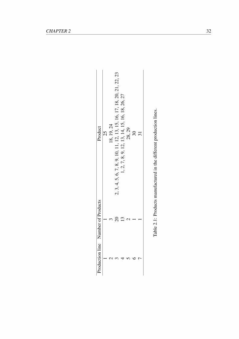
CHAPTER 2 32
Prod
uctio
nlin
eN
umbe
rofP
rodu
cts
Prod
uct
11
252
318
,19,
243
202,
3,4,
5,6,
7,8,
9,10
,11,
12,1
3,15
,16,
17,1
8,20
,21,
22,2
34
131,
2,7,
8,9,
12,1
3,14
,15,
16,1
8,26
,27
52
28,2
96
130
71
31
Tabl
e2.
1:Pr
oduc
tsm
anuf
actu
red
inth
edi
ffer
entp
rodu
ctio
nlin
es.
CHAPTER 2 33
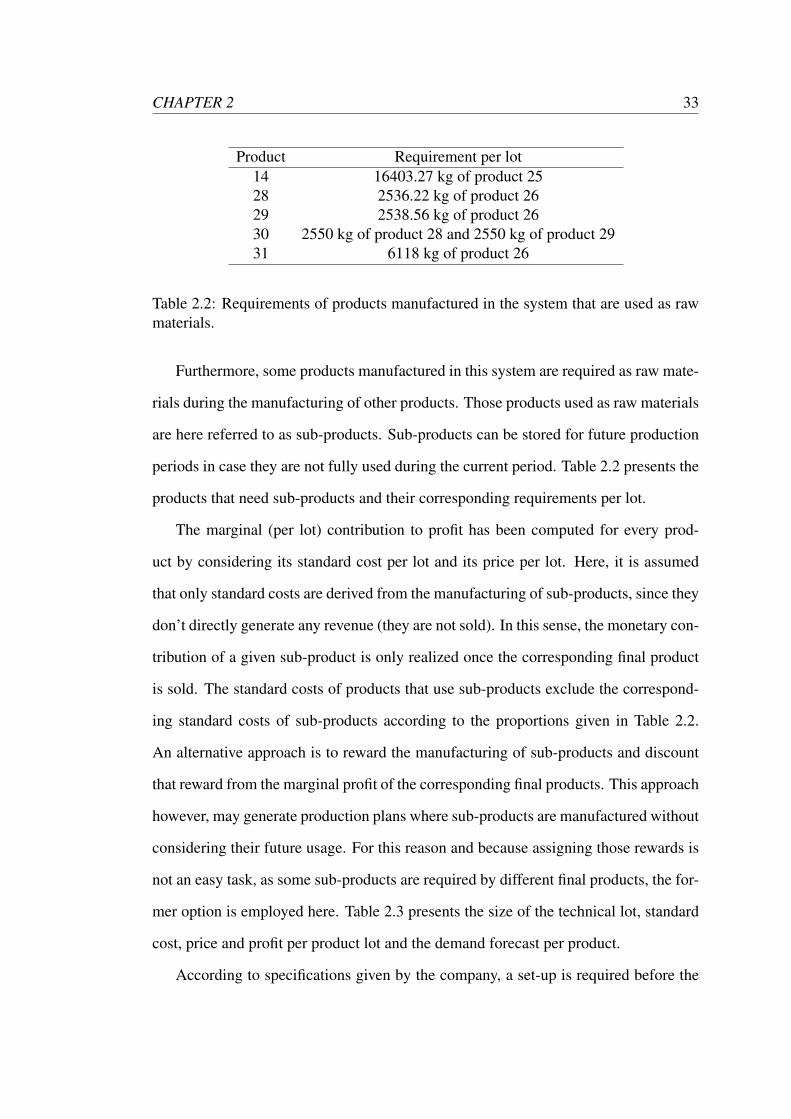
Product Requirement per lot14 16403.27 kg of product 2528 2536.22 kg of product 2629 2538.56 kg of product 2630 2550 kg of product 28 and 2550 kg of product 2931 6118 kg of product 26
Table 2.2: Requirements of products manufactured in the system that are used as rawmaterials.
Furthermore, some products manufactured in this system are required as raw mate-
rials during the manufacturing of other products. Those products used as raw materials
are here referred to as sub-products. Sub-products can be stored for future production
periods in case they are not fully used during the current period. Table 2.2 presents the
products that need sub-products and their corresponding requirements per lot.
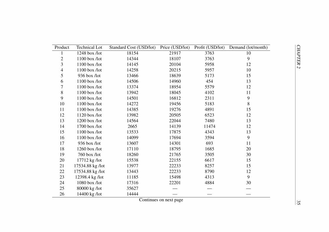
The marginal (per lot) contribution to profit has been computed for every prod-
uct by considering its standard cost per lot and its price per lot. Here, it is assumed
that only standard costs are derived from the manufacturing of sub-products, since they
don’t directly generate any revenue (they are not sold). In this sense, the monetary con-
tribution of a given sub-product is only realized once the corresponding final product
is sold. The standard costs of products that use sub-products exclude the correspond-
ing standard costs of sub-products according to the proportions given in Table 2.2.
An alternative approach is to reward the manufacturing of sub-products and discount
that reward from the marginal profit of the corresponding final products. This approach
however, may generate production plans where sub-products are manufactured without
considering their future usage. For this reason and because assigning those rewards is
not an easy task, as some sub-products are required by different final products, the for-
mer option is employed here. Table 2.3 presents the size of the technical lot, standard
cost, price and profit per product lot and the demand forecast per product.
According to specifications given by the company, a set-up is required before the

CHAPTER 2 34
manufacture of every product lot. A set-up is required even between consecutive lots
of the same product. This is due to the nature of the operations undertaken in this
manufacturing system. For instance, due to safety measures a deep cleaning of certain
production line components has to be performed before processing a new lot, even if
it is a lot of the same product, in order to remove chemical compounds (formed during
manufacturing) that could react with raw materials (e.g. exothermic reactions).
CH
AP
TER
235
Product Technical Lot Standard Cost (USD/lot) Price (USD/lot) Profit (USD/lot) Demand (lot/month)1 1248 box /lot 18154 21917 3763 102 1100 box /lot 14344 18107 3763 93 1100 box /lot 14145 20104 5958 124 1100 box /lot 14258 20215 5957 105 936 box /lot 13466 18639 5173 156 1100 box /lot 14506 14960 454 137 1100 box /lot 13374 18954 5579 128 1100 box /lot 13942 18045 4102 119 1100 box /lot 14501 16812 2311 9
10 1100 box /lot 14272 19456 5183 811 1100 box /lot 14385 19276 4891 1512 1120 box /lot 13982 20505 6523 1213 1200 box /lot 14564 22044 7480 1314 1700 box /lot 2665 14139 11474 1215 1100 box /lot 13533 17875 4343 1316 1100 box /lot 14099 17694 3594 917 936 box /lot 13607 14301 693 1118 1260 box /lot 17110 18795 1685 2019 760 box /lot 18260 21765 3505 3020 17712 kg /lot 15538 22155 6617 1521 17534.88 kg /lot 13977 22233 8257 1522 17534.88 kg /lot 13443 22233 8790 1223 12398.4 kg /lot 11185 15498 4313 924 1080 box /lot 17316 22201 4884 3025 80000 kg /lot 35627 — — —26 14400 kg /lot 14444 — — —
Continues on next page
CH
AP
TER
236
Product Technical Lot Standard Cost (USD/lot) Price (USD/lot) Profit (USD/lot) Demand (lot/month)27 14300 kg /lot 15431 15544 114 1028 2700 kg /lot 432 — — —29 2700 kg /lot 416 — — —30 5000 kg /lot 556 6847 6290 1031 5940 kg /lot 488 6077 5588 10
Table 2.3: Product lot characteristics and demand level.
CHAPTER 2 37
Moreover, the technical lot1 of every product is fixed and it has been specified by
the company so that an entire lot can be manufactured within one shift. Here, a shift
has a length of 8 hours, which corresponds to the daily amount of hours that an operator
needs to work. Therefore, the theoretical manufacturing time for every product lot is 8
hours (if everything goes well). This theoretical manufacturing time already considers
set-up time and time spent in transportation of necessary resources to and within the
production line involved, but it does not consider unexpected events such as delays
caused by failures of production lines.
In this manufacturing system, each operator needs to perform a wide variety of
operations and needs to possess the skills required to operate the different components
of the multiple production lines; for this reason any operator can be assigned to work in
any of the 7 production lines. This system has available a total of 7680 man hours per
working month (24 working days). Labour is a limiting factor of this manufacturing
system, but due to the high level of skills required it is not possible to increase the
capacity of the manufacturing system by hiring additional personnel, at least not in
the short term. Specifications about the number of man hours and hours of production
lines needed to manufacture one product lot are given in Table 2.4.
Maximum 3 shifts, of 8 hours each, can be undertaken per day at each production
line, depending on the amount of labour available. Thus, without considering labour,
the monthly design capacity (Heizer et al., 2004, p. 252) of every production line is 72
lots or 576 hours if expressed as a production rate or as the number of hours that the
production line is available, respectively.
Based on the design capacities of production lines, on the number of man hours
available and on the monthly level of demand, this system has insufficient capacity to
fully cover demand requirements. Market conditions do not allow backordering, since
any unmet demand is covered by competitors. Additionally this manufacturing system
1the number of items produced per lot of product
CHAPTER 2 38
Product Labour Requirement (h/lot) Production Line Requirement (h/lot)1 72 82 64 83 64 84 64 85 56 86 64 87 64 88 64 89 64 8
10 64 811 64 812 64 813 56 814 40 815 64 816 64 817 56 818 40 819 48 820 64 821 64 822 64 823 56 824 64 825 40 826 40 827 40 828 32 829 32 830 32 831 16 8
Table 2.4: Requirements of labour and production lines per product lot.
CHAPTER 2 39
is subject to failures of production lines, which further complicates the situation.
Historical records from January 2010 to June 2014 were obtained about the number
of failures occurred per production line during that period as well as the correspond-
ing repair times measured in days caused by each production line failure. However,
no records could be obtained for the number of lots manufactured during that period
in the different production lines. For this reason we could not calculate the exact
probability that a failure occurs in a production line during the manufacturing of a
product lot. Nevertheless, a conservative lower bound for such probability was calcu-
lated for every production line, based on the historical information mentioned above
and by considering that every production line was fully utilized (without considering
labour requirements) and reliable (no failures) during a period of 54 months (number
of months for which information is available). In other words, it was assumed that ev-
ery production line produced monthly 72 lots during 54 months, which is an unrealistic
(too optimistic) assumption, since labour constraints and the occurrence of failures in
production lines are completely ignored. For this reason, it is reasonable to consider
that actual values for those probabilities should be higher than the ones reported in
Table 2.5, which presents those conservative probabilities as well as the average repair
times per production line. As can be seen in Table 2.5, no failures were recorded for
production lines 1 and 6 during that 54-month period.
All activities in a production line stop after the occurrence of a failure and are
resumed once the repair service on that line has been completed. The delays caused
by repair services compromise the realization of a given production plan, as lots at the
end of the production sequence scheduled for that line might not be completed on time.
In terms of labour, workers assigned to that production line are idle until it becomes
operative again. When this happens, the workers on that shift resume operations until
the end of their shift and leave the remaining activities to be completed by workers
from the subsequent shift. Therefore, the occurrence of production line failures may
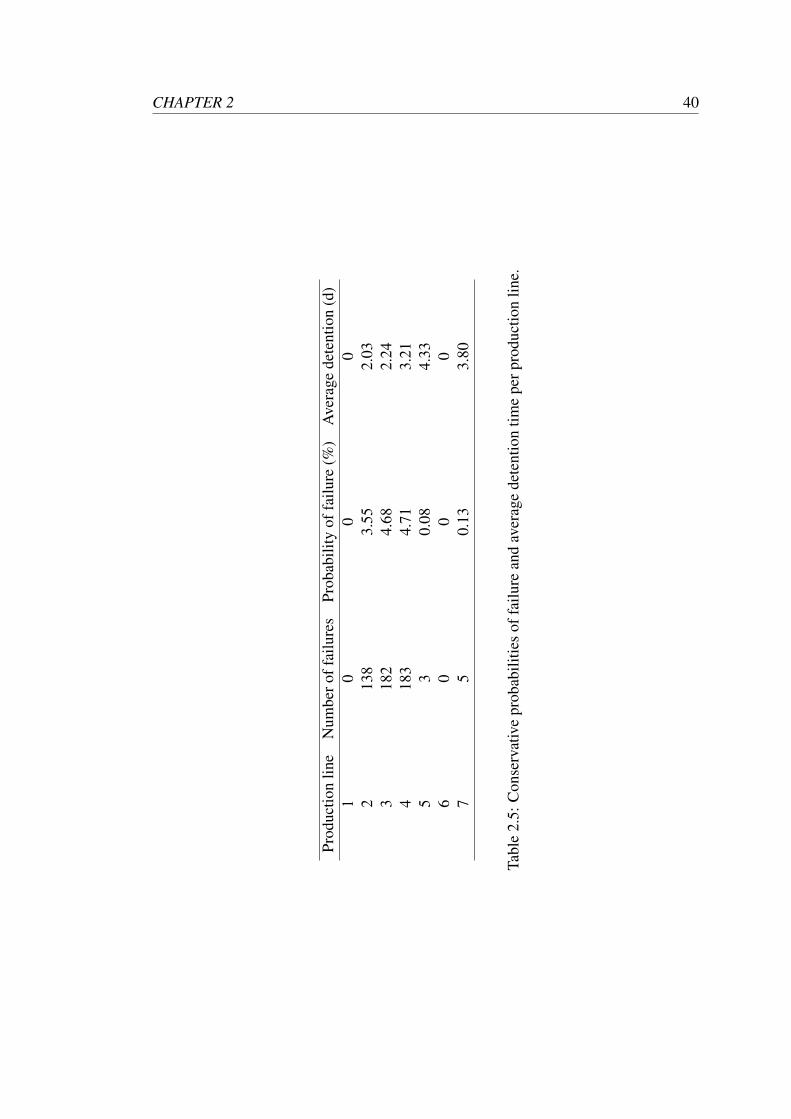
CHAPTER 2 40
Prod
uctio
nlin
eN
umbe
roff
ailu
res
Prob
abili
tyof
failu
re(%
)A
vera
gede
tent
ion
(d)
10
00
213
83.
552.
033
182
4.68
2.24
418
34.
713.
215
30.
084.
336
00
07
50.
133.
80
Tabl
e2.
5:C
onse
rvat
ive
prob
abili
ties
offa
ilure
and
aver
age
dete
ntio
ntim
epe
rpro
duct
ion
line.
CHAPTER 2 41
force to produce a given product lot within different shifts, although the technical lot
of every product has been specified with the intention of manufacturing a product lot
within a single shift. In this sense, having the possibility to make decisions about the
sizes of technical lots may bring more flexibility to improve the performance of this
manufacturing system. Moreover, assigning new tasks to idle workers are also other
important decisions, which can be made to improve the performance of this system.
However, lot-sizing and re-allocation of labour are outside the scope of this study as
those are decisions taken at the operational level rather than at the tactical level.
This company needs to purchase the materials needed for the next working month,
before the beginning of the production period, and thus a production plan for the fol-
lowing month must be available in order to make adequate purchasing decisions. This
is a difficult task because by the time a production plan needs to be developed specific
due dates of orders are still unknown and only demand forecasts are available. This
manufacturing company develops those tactical production plans on a monthly basis
and the generation of those plans is responsibility of the production planning commit-
tee (PPC).
2.2 Production Planning Challenges
One difficulty faced by this manufacturing system is that production plans are devel-
oped with the sole intention of maximizing company’s profitability. Other important
criteria such as robustness of production plans are not considered during the specifica-
tion of production plans (the failure to consider the multi-objective nature of produc-
tion planning mentioned in Section 1.1).
Also the level of detail contained in monthly production plans poses challenges to
their implementation. Plans specified by the PPC only indicate the number of lots to
produce for the different products, but they do not specify in what production lines
CHAPTER 2 42
those product lots should be manufactured (the aggregation principle mentioned in
Section 1.1). Not having the latter information causes serious difficulties during the
implementation of those plans, mainly due to overestimation of system capacity.
One of the main difficulties faced by this manufacturing system is the consideration
of system constraints during the development of monthly production plans. System
constraints are considered by the PPC via simple rules of thumb (the use of unrealistic
assumptions mentioned in Section 1.1). Moreover, this committee does not consider
from the very beginning the capacity needed to manufacture sub-products. Those con-
siderations are only made after a preliminary plan has been obtained, which is then
revised to account for the lots of sub-products needed.
Finally, the inherent uncertainty of the manufacturing system is not taken into ac-
count by the PPC. For instance, the uncertainty around potential delays caused by the
occurrence of production line failures are not considered during the specification of a
production plan (the use of unrealistic assumptions mentioned in Section 1.1).
There is a clear correspondence between the difficulties mentioned in Section 1.1
and the challenges faced by this company, which suggests that those challenges may
be the consequence of methodological limitations.
2.3 Production Planning Problem
In order to overcome the challenges mentioned in Section 2.2, the monthly produc-
tion planning of this company is addressed in this work as an optimization problem
that tries to determine the number of lots of the different products and sub-products
that every production line needs to manufacture, during a finite planning horizon of
one month, in order to simultaneously optimize at least two conflicting criteria, the
profitability and robustness of production plans. The uncertainty derived from failures

CHAPTER 2 43
in production lines, as well as complex features, such as the multi-product, multi-
production line, and multi-level nature of the manufacturing system, needs to be ac-
curately incorporated into the problem formulation in order to generate feasible and
applicable solutions. Considering all these requirements, this problem corresponds to
a multi-objective, big bucket, multi-product, multi-level (sub-products), capacitated
(constraints are considered) production planning problem of a failure-prone manufac-
turing system, conformed by multiple production lines with insufficient capacity to
fully cover demand requirements.
Chapter 3
Initial Simulation-Based Optimization
Model (Manuscript 1)
J. E. Diaz and J. Handl. Simulation-based GA optimization for production planning. In
Bioinspired Optimization Methods and their Applications, pages 27-39. Jozef Stefan
Institute, 2014.
3.1 Abstract
Effective production planning requires models that are capable of accounting for the
complexity and uncertainty intrinsic to manufacturing systems. While the identifi-
cation of a globally optimal plan is desirable, a more important requirement is the
ability of a model to produce production plans that are sufficiently realistic to be im-
plemented in practice and are robust to perturbations in the system. Here, we present
a simulation-based optimization approach that employs DES and a GA as a method-
ology to support decision making in the area of production planning. The model aims
to minimize the sum of expected backorders and inventory costs, while incorporating
system constraints and the uncertainty that derives from variations of manufacturing
44
CHAPTER 3 45
lead times, occurrence of production line failures and repair service times. Preliminary
results for a real-world problem indicate that the model is capable of producing feasible
production plans that correctly account for the uncertainty intrinsic to the underlying
manufacturing system.
3.2 Introduction
Production planning, which specifies how resources should be allocated to production
activities (Monostori et al., 2010), forms an integral part of medium-term planning
within manufacturing processes. Given the increasing pressures faced by manufac-
turers, the development and deployment of effective models that support production
planning is essential.
Ideally, an optimal production plan should be able to achieve customer satisfac-
tion (Pochet, 2001) along with profit maximization, while considering the uncertainty
in the system (Monostori et al., 2010; Li et al., 2004). Therefore, an appropriate
methodology needs to perform optimization while accounting for the effects that un-
certain parameters may have on the implementation of a production plan. This should
then lead to an optimized solution that is robust towards various sources of uncertainty
in the manufacturing system. The lack of an instrument that is fully able to meet this
requirement is one of the main reasons why, currently, decisions in production plan-
ning are often made in a subjective manner (based on the experience and “sixth sense”
of a few people) or guided by inappropriate methodologies.
Optimization and simulation models have been previously deployed to solve pro-
duction planning problems, albeit independently. Optimization models are able to gen-
erate optimal or near-optimal solutions, but the real applicability of these solutions is
often limited. This is because of the oversimplifying assumptions made by many exact
optimization models and their inability to fully incorporate uncertainty (Gnoni et al.,
CHAPTER 3 46
2003; Nikolopoulou and Ierapetritou, 2012). Furthermore, when trying to incorporate
the high level of complexity and the stochastic (Lacksonen, 2001) and dynamic na-
ture of manufacturing systems (Azzaro-Pantel et al., 1998) into optimization models,
standard approaches become computationally intractable. On the other hand, simu-
lation approaches are capable of capturing the uncertainty of the system (Monostori
et al., 2010) and of accurately reproducing its behaviour (Hsieh, 2002). Therefore,
simulation often provides a better representation of a real production system, since
the variability introduced through exogenous and endogenous factors can be explic-
itly considered and the impact of these factors can be assessed (April et al., 2006).
However, in contrast to optimization approaches, the results obtained from simulation
models are fundamentally descriptive: while a clear picture of the system is obtained,
the results do not provide explicit guidance towards improved solutions.
In an attempt to combine the respective advantages of simulation and optimization
techniques, SBO has been suggested as a means of handling problems where the high
level of complexity precludes a complete analytic formulation and the ultimate goal is
the identification of a robust, near-optimal solution (Gray et al., 2010). More specifi-
cally, the combined application of DES and GAs has been successfully applied to ad-
dress several problems related to manufacturing systems. For instance, Azzaro-Pantel
et al. (1998) were able to improve the efficiency of a multi-purpose, multi-objective
plant with limited storage by accurately modelling the dynamic behaviour of the pro-
duction system through DES and solving the scheduling problem using a GA. Al-
Aomar (2006) combined DES and a GA to determine robust design parameters. The
author integrated Taguchis’s robustness measures of signal-to-noise ratio and the qual-
ity loss function into a GA in order to enhance the selection scheme. Ding et al. (2005)
employed DES to capture the uncertainty involved in the supplier selection process and
used a GA to optimize the supplier portfolio. Cheng and Yan (2009) applied an integra-
tion of DES and a messy GA to determine the near optimal combination of resources
CHAPTER 3 47
in order to enhance the performance of construction operations. This approach enabled
the authors to cope with the complexity and large dimensionality of the problem and to
obtain adequate solutions. Wu et al. (2011) integrated DES with a GA to determine the
order point for different product types of a cross-docking center in order to minimize
total cost. Through this approach the solution space was efficiently reduced and more
simulation effort was allocated to promising areas via smart computing budget alloca-
tion. Korytkowski et al. (2013) proposed an evolutionary simulation-based heuristics,
where DES and a GA were deployed to find near optimal solutions for dispatching
rules allocation. The sequence of orders determined through this approach improved
the performance of a complex multi-stage, multi-product manufacturing system.
Here, we describe a SBO approach for production planning. The long-term aim of
our work is to derive an effective modelling approach that is capable of determining
feasible and robust monthly production plans. Here, we formulate production planning
as an optimization problem that requires the minimization of the expected sum of back-
orders and inventory costs, subject to a set of constraints of the manufacturing system
(e.g. resource constraints) and uncertainties deriving from variations of manufactur-
ing lead times, occurrence of production line failures and repair service times. Our
choice of methodology is motivated by the proven success of SBO in related problems
(see Korytkowski et al. (2013), Wu et al. (2011), Cheng and Yan (2009), Al-Aomar
(2006), Ding et al. (2005), Azzaro-Pantel et al. (1998) and above), and we develop a
model based on the combination of DES and a meta-heuristic optimizer (specifically,
a GA). Finally, we describe preliminary results on a real-world production planning
problem.
CHAPTER 3 48
3.3 Simulation-based Optimization Model
The production planning problem considered here is based on the real manufacturing
system of a large company that specializes in the production of cleaning products,
edible shortenings, fats and oils. This study focuses exclusively on its activities related
to the manufacturing of cleaning products.
DES is a good option to model the dynamic behaviour of this production sys-
tem (Azzaro-Pantel et al., 1998), as it allows for the incorporation of stochastic events
and the variations of processes that occur in complex systems (Riley, 2013). Specif-
ically, the use of DES enables us to capture the uncertainty intrinsic to production
planning that cannot be represented by deterministic models (Monostori et al., 2010).
The application of SBO implies the absence of an analytical problem formulation,
i.e. the functional relationships between dependent and independent variables are not
known explicitly (Steponavice et al., 2014). Consequently, a suitable optimization
approach needs to be able to perform optimization based exclusively on function values
obtained via simulation, a so called “black-box approach”. Considering the complexity
and large dimensionality of the solution space, a suitable search strategy should be able
to find near-optimal solutions in a large and complex solution space and be capable of
escaping local optima. Finally, the optimization method needs to be robust with respect
to noise, since the optimization procedure relies on stochastic responses generated by
the simulation model (Gray et al., 2010). Meta-heuristics present suitable candidates
for this setting, and in this study, a GA was selected as the optimizer. This choice
was motivated by previous research indicating the robust performance of GAs under
noisy conditions (Mitchell, 1998; Baum et al., 1995), specifically, in the context of
DES optimization (Lacksonen, 2001).
The DES model of the production system was developed in SimEventsr (The
MathWorks, Inc., 2013). This was integrated with Matlabr R2013a (The MathWorks,
CHAPTER 3 49
Inc., 2013), and Matlab’s standard GA implementation was employed as the optimizer.
Details of the simulation model and optimizer are described in the following sections.
3.3.1 Simulation Model
The DES model represents the production of 31 products j within 7 production lines
l. A production line corresponds to the set of resources (e.g. machines, people, etc.)
needed to manufacture certain products. Given that some products can be manufac-
tured in several production lines a total of 41 processes y are considered in the DES
model. A process y includes all series of events involved in the initialization of orders
of a product j, its manufacture in a specific production line l and its storage in an spe-
cific container, denoted as sink (with sink = 1,2, . . . ,41). Here orders are measured in
number of lots. The simulation time t of each simulation replication is 24 days, which
corresponds to the number of working days in a month.
The model component designed for the generation of orders for a single production
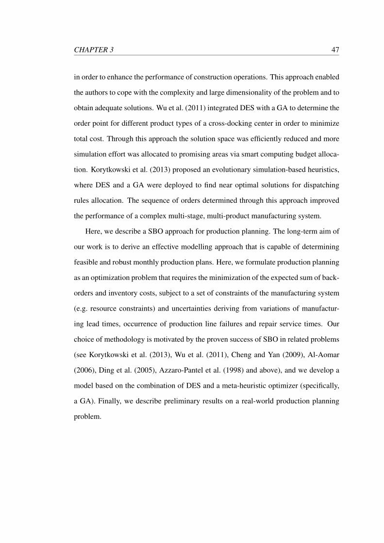
line l is illustrated in Figure 3.1. A production plan is a vector of decision variables
xy, which are specified by a GA. The values of the different decision variables are
the inputs for the simulation model (function-call generator blocks). Given that some
products j are required as raw materials during the manufacturing process of other
products j, a higher priority is assigned to the initialization of orders for those sub-
products in order to assure the static logic of the model.
Attributes are assigned to the different product lots (via attribute blocks). Speci-
fications about the containers (sink), where final products will be stored, are assigned
via an attribute called Out putPorty. Furthermore, the time required to manufacture a
specific product lot (Manu f acturingTimey) and the occurrence of a failure in a pro-
duction line while processing a product lot (ProductionLineFailurey) are additional
attributes assigned to each lot of product. Two different event-based random number
CHAPTER 3 50
Figure 3.1: Order processing subsystem for production line l.
generators are employed to set the last two attributes mentioned. Both event-based
random number generators produce a signal sampled randomly from the probability
distribution functions (PDFs) assigned to them. A synthetic data set was employed
CHAPTER 3 51
to estimate PDFs for each stochastic variable included in the current study, as data
collection for these aspects of the system is currently incomplete.
Once the attributes have been assigned to the production orders, those orders are
transferred to a queue following a first-in first-out (FIFO) discipline. Subsequently,
those queues of production orders that have to be processed by the same production
line are merged (by a path combiner block) into a single FIFO queue.
The model components of a production subsystem and repair service centre are
illustrated in Figure 3.2 and Figure 3.3, respectively. Each order is manufactured as
soon as the corresponding production line (represented by an N-server block) becomes
available. In case of failure, the activity of that production line is blocked by the
control signal Pausel. This signal is generated from the corresponding repair service
centre and it outputs the number of entities present in that repair centre. Therefore, a
signal with value greater than zero indicates that the production line l is being repaired
and stops its activity until that signal becomes zero (no entities present in the repair
service centre).
In case that no failure occurs (ProductionLineFailurey = 1), the production batch is
transferred to the corresponding container (sink) determined by Out putPorty). Whereas
if a failure occurs (ProductionLineFailurey = 2), that product batch is transferred to
a repair service centre prior to its storage. The delay caused by the production line
failure is sampled from the corresponding PDF assigned to RepairServiceTimel . One
important assumption made is that after a production batch has left the repair service
centre no re-manufacture is required, since the manufacturing process has been already
completed (passed through the N-server block). This is an effective way to model sys-
tem failure without having conflicting events.
The stock of product j manufactured in production line l, denoted by sl, j, is com-
puted at the end of every replication and it is measured in number of lots. Based on sl, j,
CHAPTER 3 52
Figure 3.2: Production subsystem for production line l.
CHAPTER 3 53
Figure 3.3: Repair service centre of production line l.
the total stock of product j (s j) is calculated at the end of every replication as follows:
s j =7
∑l=1
sl, j. (3.1)
3.3.2 Optimization Model
The decision variables, denoted by xy, are the number of lots to be produced in process
y. A black box optimization approach is applied in which the decision variables speci-
fied by the GA provide the input to the DES model and the responses s j from the DES
model are employed to compute the value of the fitness function. A total of 41 decision
variables xy, which are constrained to be positive integers, are considered in the model.
Given the stochastic nature of the DES outputs, fitness is evaluated across γ indepen-
dent simulation trials (with γ = 10). Specifically, the fitness value f is estimated for
each individual x as follows:
f (x) =1γ
γ
∑r=1
31
∑j=1
InventoryCost j,r +BackorderCost j,r, (3.2)
where InventoryCosts j,r and BackorderCosts j,r are computed based on the rth simu-
lated response s j,r as follows:
InventoryCost j,r =
(s j,r−D j)×Cost j if s j,r > D j
0 if s j,r ≤ D j
CHAPTER 3 54
and
BackorderCost j,r =
(D j− s j,r)×Price j if s j,r < D j
0 if s j,r ≥ D j
where, D j indicates the demand for product j. Unsold amounts of product j are penal-
ized proportionally to the corresponding standard cost per lot (Cost j), whereas backo-
rders receive a fine equal to the product price, which is the income lost (Price j) for not
selling that specific amount of product. Given a lack of information on real inventory
costs and total cost derived from backorders per product (cost of customer dissatisfac-
tion, cost of non-future purchases, cost of customers switching to other brands, etc.),
standard costs and product prices are currently employed to penalize inventory and
backorders, respectively. These two assumptions are not valid in reality for several
reasons. First, excess of inventory can be sold in future periods and inventory costs are
not equal to standard costs. Second, considering product price as the total loss caused
by product backorders is inaccurate and unrealistic.
Additional constraints are imposed given that some products j are required as raw
materials during the manufacturing process of other products j. Therefore, the require-
ment of sub-products is represented through linear constraints as follows:
41
∑y=1
ai,y× xy ≤ bi (i = 1,2, . . . ,4), (3.3)
where bi denotes the quantity available of sub-product i and ai,y is the amount required
of sub-product i to produce one lot in process y.
Here, we use as optimizer the default Matlab implementation for solving integer
and mixed integer problems using a GA. This is a real-coded GA that has a popula-
tion size of 50 individuals and employs Laplace crossover (crossover probability: 0.8),
power mutation (mutation probability: 0.005) and tournament selection (tournament
size: 2) as operators. A detailed description of the GA and its truncation procedure
CHAPTER 3 55
(which ensures compliance with integer constraints after crossover and mutation) can
be found in Deep et al. (2009). The inbuilt constraint-handling approach is the param-
eter free penalty function approach proposed by Deb (2000). Elitism is implemented
in this GA by having an elite set of 1 and according to Matlab customer service, the
fitness of elite individuals is re-evaluated across generations in this default Matlab im-
plementation.
3.4 Preliminary Results
The model enables an accurate incorporation of uncertainty derived from variations
of manufacturing lead times, occurrence of production line failures and repair service
times. The time required to run 15 iterations of the GA is 12.15 hours. For this reason,
very limited results are reported in the present study, and we mostly focus on the valid-
ity of the model designed. More extensive benchmarking of the approach (including
longer optimization runs and statistics across multiple trials) is currently in progress.
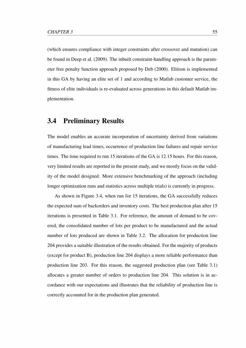
As shown in Figure 3.4, when run for 15 iterations, the GA successfully reduces
the expected sum of backorders and inventory costs. The best production plan after 15
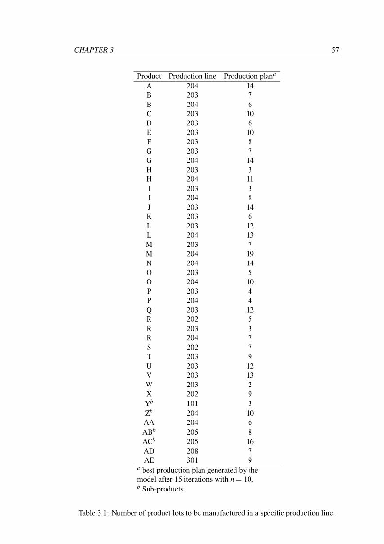
iterations is presented in Table 3.1. For reference, the amount of demand to be cov-
ered, the consolidated number of lots per product to be manufactured and the actual
number of lots produced are shown in Table 3.2. The allocation for production line
204 provides a suitable illustration of the results obtained. For the majority of products
(except for product B), production line 204 displays a more reliable performance than
production line 203. For this reason, the suggested production plan (see Table 3.1)
allocates a greater number of orders to production line 204. This solution is in ac-
cordance with our expectations and illustrates that the reliability of production line is
correctly accounted for in the production plan generated.
CHAPTER 3 56
Figure 3.4: Best, mean and worst fitness value of the population at each iteration.
3.5 Future Research
There are a number of ways in which this research will be extended in future work.
Regarding the simulation component of the work, data collection (from the company)
needs to be completed. The data obtained will be used to estimate PDFs of all stochas-
tic variables, so that the use of synthetic data can be avoided.
Regarding the optimizer, future work will include an investigation of parameter
settings, the sensitivity to noise and, potentially, the comparison to alternative meta-
heuristic optimization approaches. Moreover, the number (n) of simulation trials em-
ployed to evaluate fitness will be further analysed in order to balance quality of es-
timations and computational cost. Furthermore, a multi-objective formulation of the
problem will be explored in order to account for the robustness of solutions in a more
explicit manner. Specifically, the maximization of the signal-to-noise ratio may be
used as an additional objective to directly account for the variability in the fitness val-
ues obtained (Al-Aomar, 2006).
CHAPTER 3 57
Product Production line Production plana
A 204 14B 203 7B 204 6C 203 10D 203 6E 203 10F 203 8G 203 7G 204 14H 203 3H 204 11I 203 3I 204 8J 203 14K 203 6L 203 12L 204 13M 203 7M 204 19N 204 14O 203 5O 204 10P 203 4P 204 4Q 203 12R 202 5R 203 3R 204 7S 202 7T 203 9U 203 12V 203 13W 203 2X 202 9Yb 101 3Zb 204 10AA 204 6ABb 205 8ACb 205 16AD 208 7AE 301 9
a best production plan generated by themodel after 15 iterations with n = 10,b Sub-products
Table 3.1: Number of product lots to be manufactured in a specific production line.
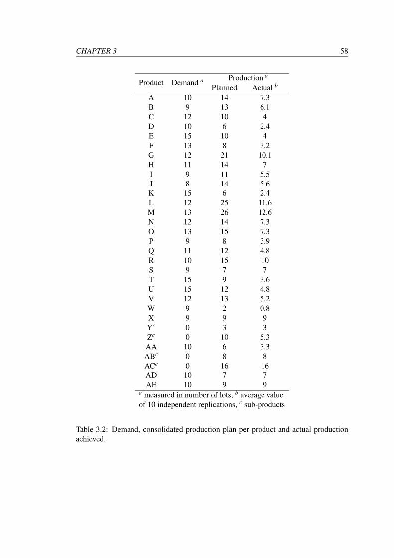
CHAPTER 3 58
Product Demand a Production a
Planned Actual b
A 10 14 7.3B 9 13 6.1C 12 10 4D 10 6 2.4E 15 10 4F 13 8 3.2G 12 21 10.1H 11 14 7I 9 11 5.5J 8 14 5.6K 15 6 2.4L 12 25 11.6M 13 26 12.6N 12 14 7.3O 13 15 7.3P 9 8 3.9Q 11 12 4.8R 10 15 10S 9 7 7T 15 9 3.6U 15 12 4.8V 12 13 5.2W 9 2 0.8X 9 9 9Yc 0 3 3Zc 0 10 5.3AA 10 6 3.3ABc 0 8 8ACc 0 16 16AD 10 7 7AE 10 9 9
a measured in number of lots, b average valueof 10 independent replications, c sub-products
Table 3.2: Demand, consolidated production plan per product and actual productionachieved.
Chapter 4
Noise Handling Strategies
(Manuscript 2)
J. E. Diaz and J. Handl. Implicit and explicit averaging strategies for simulation-based
optimization of a real-world production planning problem. Informatica: An Interna-
tional Journal of Computing and Informatics, 39(2):161–168, 2015.
4.1 Abstract
In this chapter, we explore the impact of noise handling strategies on optimization
performance in the context of the real-world production planning problem analysed
in the previous chapter. Uncertainties intrinsic to the production system are captured
using a modified version of the DES model presented in Chapter 3 (see Section 4.3.1
for further details about those modifications), and the production plan is optimized
using an EA. Unlike Chapter 3, here we aim for profit maximization rather than for
cost minimization as this is the objective that the manufacturing company intends to
optimize. The stochastic nature of the fitness values (as returned by the DES simula-
tion) may impact on optimization performance, and we explore explicit and implicit
59
CHAPTER 4 60
averaging strategies to address this issue. Specifically, we evaluate the effectiveness
of different strategies, when a limited budget of evaluations is available. Our results
indicate a general advantage of implicit averaging in this setting, and a good degree
of robustness with regard to population size. On the other hand, explicit averaging is
found to be non-competitive, due to the cost of repeat-evaluations of the same solu-
tion. Finally, we explore a hybrid approach that uses explicit averaging to refine fitness
estimates during final solution selection. Under increasing levels of fitness variability,
this hybrid strategy starts to outperform pure implicit and explicit averaging strategies.
4.2 Introduction
Optimization problems that include uncertainty pose challenges that are difficult to ad-
dress using standard optimization methodologies. While a portion of the optimization
literature is concerned with the development of methodologies capable of identify-
ing optimal solutions to problems with uncertainty, the application of these methods
often requires stringent assumptions and/or simplifications that are necessary to sat-
isfy relevant optimality conditions. Those methods are often insufficiently powerful to
accurately incorporate the full complexity and uncertainty intrinsic to real-world prob-
lems into the problem formulation, even when their consideration is essential for the
generation of reliable and feasible solutions. For this reason, solutions obtained from
traditional approaches (such as fuzzy, stochastic and stochastic dynamic programming)
to optimization problems under uncertainty may often be of limited value in producing
realistic solutions for real-world problems.
SBO constitutes an interesting alternative in situations where the high level of com-
plexity precludes a complete analytic formulation of a problem (Ehrenberg and Zim-
mermann, 2012) and where uncertainty needs to be considered (Figueira and Almada-
Lobo, 2014). The SBO model used here consists of a detailed simulation model, which
CHAPTER 4 61
is then coupled with an optimizer in a black-box fashion. In other words, the optimizer
operates on a (sub-)set of model parameters and the optimization process is based
exclusively on the (usually stochastic) simulation responses. EAs are well-suited to
black-box optimization settings, as highlighted by their wide application to real-world
optimization problems that cannot be handled by analytical approaches (Qian et al.,
2014). The feasibility and reliability of solutions become the primary consideration in
such settings (Figueira and Almada-Lobo, 2014), and the EAs’ flexibility in this re-
spect typically offsets its disadvantages (specifically, the lack of guaranteed optimality
of its identified solutions).
When EAs are employed as optimizers of SBO models, fitness values become sub-
ject to the variability arising from the stochastic responses within the simulation model.
The resulting noisy nature of the fitness values poses a challenge to the evolutionary
optimizer, for it may mislead selection procedures (Bhattacharya et al., 2014) and lead
to the propagation of inferior individuals or to the elimination of superior ones, thereby
undermining algorithm performance (Syberfeldt et al., 2010). Under these circum-
stances, noise handling strategies can play an important role in compensating for the
impact of noise on the optimizer, and, specifically, in helping the optimizer to iden-
tify solutions that exhibit low fitness variability and give rise to high average fitness.
Multiple studies have analysed situations in which noise causes perturbations during
fitness evaluation, thus generating discrepancies between the observed and “true” fit-
ness (Qian et al., 2014). We refer the reader to Jin and Branke (2005) for a compre-
hensive survey of noise handling strategies proposed in the existing literature.
Implicit and explicit averaging are the two strategies most commonly employed
to reduce the influence of noise in evolutionary optimization under noise. Implicit
averaging relies on the EA mechanism itself to compensate for the impact of noise.
Specifically, it assumes that the use of sufficiently large populations will ensure that
individuals from promising regions of the search space are sampled repeatedly (Jin and
CHAPTER 4 62
Branke, 2005; Syberfeldt et al., 2010), and the impact of noise can be reduced in this
manner. On the other hand, explicit averaging strategies ensure that individuals are
evaluated using average fitness values obtained across a specific number (n) of fitness
evaluations (replicates). Statistically, this approach ensures that the expected error of
fitness estimates (i.e. the difference between the observed and the “true” fitness mean)
reduces with a factor of√
n (Jin and Branke, 2005).
Both implicit and explicit averaging strategies incur additional fitness evaluations
due to (i) the increase in population size and due to (ii) the increase in the number of
trials, respectively. Fitness evaluations present an important consideration in SBO, as
each replication of a simulation is time-consuming and the number of these replica-
tions may be limited by available computational time. Here, we investigate the effi-
ciency and effectiveness of different noise-handling strategies in a realistic SBO set-
ting, in which the computational budget available for the optimization (and therefore,
the overall number of simulation replicates) is limited. Specifically, we compare ex-
plicit averaging against implicit averaging strategies for two different population sizes.
Finally, we investigate a hybrid scheme that aims to combine the strengths of both
approaches.
The remainder of this chapter is organized as follows. Section 4.3 introduces the
real-world optimization problem considered and the corresponding SBO model devel-
oped in this study. Explicit averaging, implicit averaging and a hybrid strategy com-
bining both approaches are described in Section 4.4. Section 4.5 presents details about
the comparative analysis, and empirical findings are presented in Section 4.6. Overall
conclusions, limitations of this study and future research directions are discussed in
Sections 4.7 and 4.8, respectively.
CHAPTER 4 63
4.3 Simulation-Based Optimization Model
In this study, a SBO approach based on the integration of DES and a GA is applied to
address the production planning problem of a real manufacturing company presented in
Chapter 3 with the difference that, here, the objective is to achieve profit maximization.
Additional modifications made to the original DES and optimization models presented
in Chapter 3 are stated in Sections 4.3.1 and 4.3.2, respectively.
This problem corresponds to a big bucket, multi-product, multi-level (sub-products),
capacitated (constraints are considered) production planning problem of a failure-prone
manufacturing system, consisting of multiple production lines with insufficient capac-
ity to fully cover demand requirements.
The DES model was developed in SimEventsr (The MathWorks, Inc., 2014) and
Matlab’s GA (MI-LXPM) implementation (Deep et al., 2009) was used as the opti-
mizer. This is the default Matlabr R2014a’s (The MathWorks, Inc., 2013) imple-
mentation for solving integer and mixed integer problems with GA. This GA employs
Laplace crossover(crossover probability: 0.8), power mutation (mutation probability:
0.005) and binary tournament selection as operators. Information about population
size and number of generations is presented in Section 4.4. The truncation procedure,
which ensures compliance with integer constraints after crossover and mutation, is de-
scribed in Deep et al. (2009). The inbuilt constraint-handling method is the parameter
free penalty function approach proposed by Deb (2000). In this GA, elitism is imple-
mented by having an elite set of 1. Please note that elite individuals are re-evaluated
during the next generation, according to Matlab customer service.
All computations were executed in parallel on a 12 core Intel(R) Xeon(R) CPU
L5640 @ 2.27GHz with 24 GB of RAM running Scientific Linux, release 6.2.
CHAPTER 4 64
4.3.1 Simulation Model
The DES model employed in this study is a modified version of the model presented
in Chapter 3.
The DES model represents the production of 31 products j within 7 production
lines l. A production line corresponds to the set of resources (e.g. machines, people,
etc.) needed to manufacture certain products. Given that some products can be manu-
factured in several production lines a total of 41 processes y are considered in the DES
model. A process y includes all series of events involved in the initialization of orders
of a product j, its manufacturing in a specific production line l and its storage in an
specific container, denoted as sink (with sink = 1,2, . . . ,41).
This model intends to capture the delays caused by production line failures and
provides the stock of products manufactured during a production period of one month
(24 days composed of 3 shifts of 8 hours each). The total stock of a specific product
(s j) corresponds to the sum of lots manufactured across the different production lines
as shown by the following equation:
s j =7
∑l=1
sl, j, (4.1)
where sl, j is the stock of product j manufactured in production line l.
The first modification to the original simulation model is that here the manufactur-
ing time of a product lot is treated as a constant when no failure occurs, rather than as
a random variable. This is according to specifications provided by the company.
Moreover, we consider the occurrence of production line failures that are indepen-
dent of the product type. The occurrence of a failure in a production line is modelled
here by a random variable Hl , whose numerical values hl are sampled from a probabil-
ity mass function (PMF) with sample space ΩH = 0,1, where hl = 1 represents the
occurrence of a failure and hl = 0 indicates that no failure occurred. The probability
CHAPTER 4 65
that hl = 1 is pHl(1) = pl; consequently, pHl(0) = 1− pl . Here, numerical values of
Hl are sampled every time a product lot is manufactured; therefore, pl is the proba-
bility that a production line fails during the manufacturing of a product lot. After a
production line failure, a repair service needs to be carried out. The delay λl caused by
a repair service is the numerical realization of a random variable Λl , modelled by an
exponential probability density function (PDF) with known mean µl .
Finally, an additional server was added to each process in the original simulation
model, so that the first lot of every process is processed by this server during the entire
duration of each simulation replication (24 days). This modification was made to allow
decision variables to take values equal to zero, a possibility not accounted for in the
original model (Chapter 3).
4.3.2 Optimization Model
The objective here is to generate production plans that try to maximize the expected
sum of contributions to profit generated from processes undertaken by a failure-prone
manufacturing system. The expected sum of contributions to profit is later referred to
as “profit” for simplification purposes.
A total of 41 decision variables (xy) are considered, which correspond to the num-
ber of lots to be produced in each process y, and are constrained to be non-negative
integers. Those decision variables, specified by the GA, constitute the input to the
DES model which outputs the realization of those decision variables, denoted here
as s j. Those simulated responses (s j) are used to compute the fitness value of each
production plan x across γ independent simulation replicates as follows:
maximize f (x) =1γ
γ
∑r=1
31
∑j=1
v j× s j,r, (4.2)
where v j corresponds to the contribution margin per lot of product j and the value of γ
CHAPTER 4 66
varies depending on the strategy applied (see Section 4.5 for details about γ).
Additional constraints are imposed in the form of Equation 4.3 to avoid production
levels greater than the maximum demand, to represent the requirement of sub-products
and labour needed to undertake each process.
41
∑y=1
ai,y× xy ≤ bi (i = 1,2, . . . ,44), (4.3)
where bi denotes the magnitude of constraint i and ai,y corresponds to the amount
deployed from bi by manufacturing one lot in process y.
4.4 Noise Handling Strategies
In this study we focus exclusively on implicit and explicit averaging strategies, as
these are straightforward to implement in any EA and present the approaches most
commonly employed in practice. Other noise handling strategies, such as averaging
by means of approximated models (Branke et al., 2001; Neri et al., 2008; Sano et al.,
2000) and modifications of the selection scheme (Branke and Schmidt, 2003; Rudolph,
2001), have been proposed in the literature, but are not considered here.
An explicit averaging strategy uses a fixed number γ of simulation replicates to ob-
tain an average fitness value for each individual, as described in Equation 4.2. These
average fitness estimates are then used to inform selection probabilities in the EA.
Therefore, under the explicit averaging strategy (ES) here analysed, fitness of an indi-
vidual x is computed across 10 independent fitness evaluations (γ = 10) and the popu-
lation size employed corresponds to 50 individuals. γ is set at this relatively small level
because a limited computational budget of 25000 fitness evaluations is available, and
assigning higher values to γ or using a larger population size would reduce the number
of generations that can be executed under ES.

CHAPTER 4 67
In contrast, an implicit averaging strategy uses a single simulation replicate (γ = 1)
to evaluate the quality of an individual. Increased robustness towards noise is then
achieved by increasing population size relative to standard settings of this parameter.
Consequently, under the implicit averaging strategy (IS), a single fitness evaluation
(γ = 1) is used to compute fitness and a population size of 100 individuals is applied.
Additionally, a baseline strategy (BS) is also analysed in order to evaluate the per-
formance of implicit averaging when the population size is the same as in ES, and
therefore, twice as many generations are evolved compared to IS.
Moreover, we further describe a hybrid strategy (HS) that attempts to combine
aspects of implicit and explicit averaging. This strategy applies implicit averaging
(γ = 1 and a population size of 100 individuals) throughout the evolution process, but
switches behaviour towards the end of the optimization: instead of choosing the final
solution based on a single fitness value, we propose to select from the final population
the feasible individual with the best average fitness. Consequently, we implement a
mechanism that computes the average fitness of every feasible individual of the final
population across a number γ of fitness evaluations, generated from independent sim-
ulation replications. The value of γ depends on the number of feasible individuals (δ)
in the final population and on the computational budget available for this last step (E),
which in this case corresponds to 1000 fitness evaluations. γ is computed as follows:
γ =
⌊Eδ
⌋. (4.4)
Therefore, having a population size of 100, if every individual in the final popula-
tion is feasible, 10 fitness evaluations are used to compute the average fitness of each
individual. However, if unfeasible individuals are present in the final population, those
1000 fitness evaluations are distributed amongst feasible individuals only.
Parameters specified for all four noise handling strategies introduced in this section
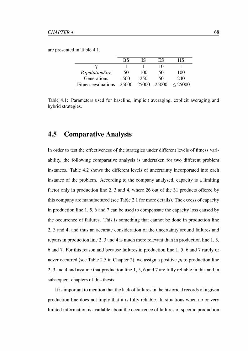
CHAPTER 4 68
are presented in Table 4.1.
BS IS ES HSγ 1 1 10 1
PopulationSize 50 100 50 100Generations 500 250 50 240
Fitness evaluations 25000 25000 25000 ≤ 25000
Table 4.1: Parameters used for baseline, implicit averaging, explicit averaging andhybrid strategies.
4.5 Comparative Analysis
In order to test the effectiveness of the strategies under different levels of fitness vari-
ability, the following comparative analysis is undertaken for two different problem
instances. Table 4.2 shows the different levels of uncertainty incorporated into each
instance of the problem. According to the company analysed, capacity is a limiting
factor only in production line 2, 3 and 4, where 26 out of the 31 products offered by
this company are manufactured (see Table 2.1 for more details). The excess of capacity
in production line 1, 5, 6 and 7 can be used to compensate the capacity loss caused by
the occurrence of failures. This is something that cannot be done in production line
2, 3 and 4, and thus an accurate consideration of the uncertainty around failures and
repairs in production line 2, 3 and 4 is much more relevant than in production line 1, 5,
6 and 7. For this reason and because failures in production line 1, 5, 6 and 7 rarely or
never occurred (see Table 2.5 in Chapter 2), we assign a positive pl to production line
2, 3 and 4 and assume that production line 1, 5, 6 and 7 are fully reliable in this and in
subsequent chapters of this thesis.
It is important to mention that the lack of failures in the historical records of a given
production line does not imply that it is fully reliable. In situations when no or very
limited information is available about the occurrence of failures of specific production
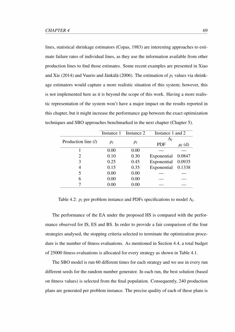
CHAPTER 4 69
lines, statistical shrinkage estimators (Copas, 1983) are interesting approaches to esti-
mate failure rates of individual lines, as they use the information available from other
production lines to find those estimates. Some recent examples are presented in Xiao
and Xie (2014) and Vaurio and Jankala (2006). The estimation of pl values via shrink-
age estimators would capture a more realistic situation of this system; however, this
is not implemented here as it is beyond the scope of this work. Having a more realis-
tic representation of the system won’t have a major impact on the results reported in
this chapter, but it might increase the performance gap between the exact optimization
techniques and SBO approaches benchmarked in the next chapter (Chapter 5).
Instance 1 Instance 2 Instance 1 and 2
Production line (l) pl plΛl
PDF µl (d)1 0.00 0.00 — —2 0.10 0.30 Exponential 0.08473 0.25 0.45 Exponential 0.09354 0.15 0.35 Exponential 0.13385 0.00 0.00 — —6 0.00 0.00 — —7 0.00 0.00 — —
Table 4.2: pl per problem instance and PDFs specifications to model Λl .
The performance of the EA under the proposed HS is compared with the perfor-
mance observed for IS, ES and BS. In order to provide a fair comparison of the four
strategies analysed, the stopping criteria selected to terminate the optimization proce-
dure is the number of fitness evaluations. As mentioned in Section 4.4, a total budget
of 25000 fitness evaluations is allocated for every strategy as shown in Table 4.1.
The SBO model is run 60 different times for each strategy and we use in every run
different seeds for the random number generator. In each run, the best solution (based
on fitness values) is selected from the final population. Consequently, 240 production
plans are generated per problem instance. The precise quality of each of these plans is
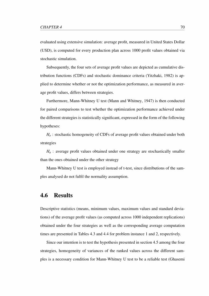
CHAPTER 4 70
evaluated using extensive simulation: average profit, measured in United States Dollar
(USD), is computed for every production plan across 1000 profit values obtained via
stochastic simulation.
Subsequently, the four sets of average profit values are depicted as cumulative dis-
tribution functions (CDFs) and stochastic dominance criteria (Yitzhaki, 1982) is ap-
plied to determine whether or not the optimization performance, as measured in aver-
age profit values, differs between strategies.
Furthermore, Mann-Whitney U test (Mann and Whitney, 1947) is then conducted
for paired comparisons to test whether the optimization performance achieved under
the different strategies is statistically significant, expressed in the form of the following
hypotheses:
Ho : stochastic homogeneity of CDFs of average profit values obtained under both
strategies
Ha : average profit values obtained under one strategy are stochastically smaller
than the ones obtained under the other strategy
Mann-Whitney U test is employed instead of t-test, since distributions of the sam-
ples analysed do not fulfil the normality assumption.
4.6 Results
Descriptive statistics (means, minimum values, maximum values and standard devia-
tions) of the average profit values (as computed across 1000 independent replications)
obtained under the four strategies as well as the corresponding average computation
times are presented in Tables 4.3 and 4.4 for problem instance 1 and 2, respectively.
Since our intention is to test the hypothesis presented in section 4.5 among the four
strategies, homogeneity of variances of the ranked values across the different sam-
ples is a necessary condition for Mann-Whitney U test to be a reliable test (Ghasemi
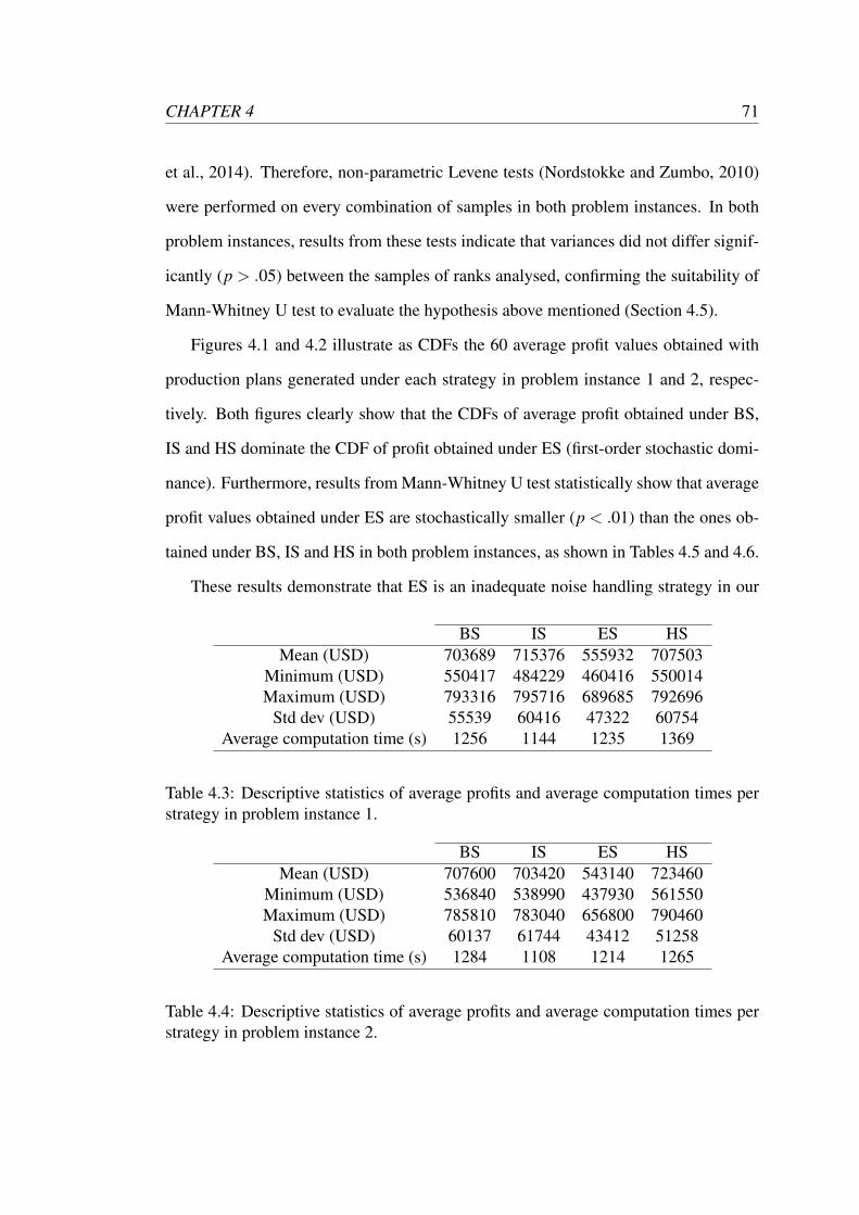
CHAPTER 4 71
et al., 2014). Therefore, non-parametric Levene tests (Nordstokke and Zumbo, 2010)
were performed on every combination of samples in both problem instances. In both
problem instances, results from these tests indicate that variances did not differ signif-
icantly (p > .05) between the samples of ranks analysed, confirming the suitability of
Mann-Whitney U test to evaluate the hypothesis above mentioned (Section 4.5).
Figures 4.1 and 4.2 illustrate as CDFs the 60 average profit values obtained with
production plans generated under each strategy in problem instance 1 and 2, respec-
tively. Both figures clearly show that the CDFs of average profit obtained under BS,
IS and HS dominate the CDF of profit obtained under ES (first-order stochastic domi-
nance). Furthermore, results from Mann-Whitney U test statistically show that average
profit values obtained under ES are stochastically smaller (p < .01) than the ones ob-
tained under BS, IS and HS in both problem instances, as shown in Tables 4.5 and 4.6.
These results demonstrate that ES is an inadequate noise handling strategy in our
BS IS ES HSMean (USD) 703689 715376 555932 707503
Minimum (USD) 550417 484229 460416 550014Maximum (USD) 793316 795716 689685 792696
Std dev (USD) 55539 60416 47322 60754Average computation time (s) 1256 1144 1235 1369
Table 4.3: Descriptive statistics of average profits and average computation times perstrategy in problem instance 1.
BS IS ES HSMean (USD) 707600 703420 543140 723460
Minimum (USD) 536840 538990 437930 561550Maximum (USD) 785810 783040 656800 790460
Std dev (USD) 60137 61744 43412 51258Average computation time (s) 1284 1108 1214 1265
Table 4.4: Descriptive statistics of average profits and average computation times perstrategy in problem instance 2.
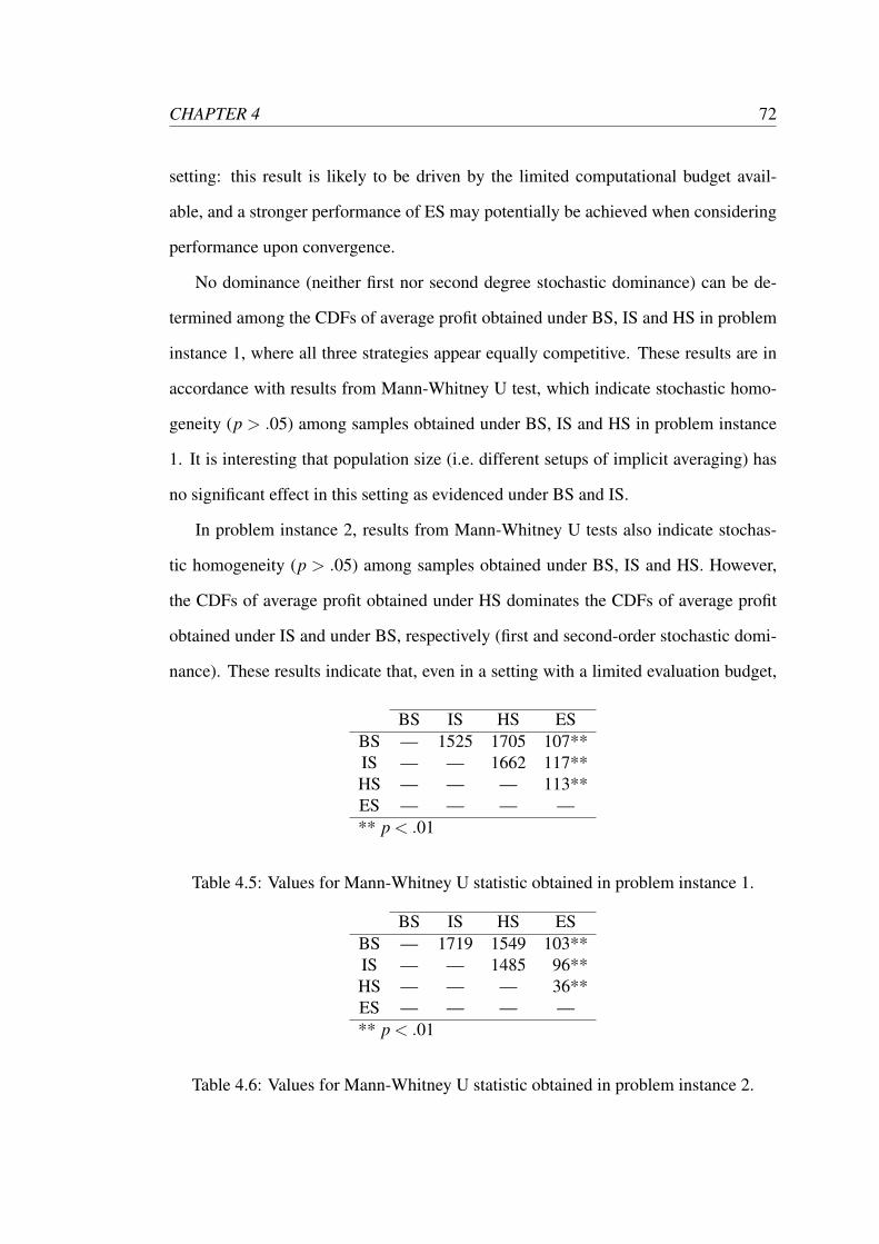
CHAPTER 4 72
setting: this result is likely to be driven by the limited computational budget avail-
able, and a stronger performance of ES may potentially be achieved when considering
performance upon convergence.
No dominance (neither first nor second degree stochastic dominance) can be de-
termined among the CDFs of average profit obtained under BS, IS and HS in problem
instance 1, where all three strategies appear equally competitive. These results are in
accordance with results from Mann-Whitney U test, which indicate stochastic homo-
geneity (p > .05) among samples obtained under BS, IS and HS in problem instance
1. It is interesting that population size (i.e. different setups of implicit averaging) has
no significant effect in this setting as evidenced under BS and IS.
In problem instance 2, results from Mann-Whitney U tests also indicate stochas-
tic homogeneity (p > .05) among samples obtained under BS, IS and HS. However,
the CDFs of average profit obtained under HS dominates the CDFs of average profit
obtained under IS and under BS, respectively (first and second-order stochastic domi-
nance). These results indicate that, even in a setting with a limited evaluation budget,
BS IS HS ESBS — 1525 1705 107**IS — — 1662 117**HS — — — 113**ES — — — —** p < .01
Table 4.5: Values for Mann-Whitney U statistic obtained in problem instance 1.
BS IS HS ESBS — 1719 1549 103**IS — — 1485 96**HS — — — 36**ES — — — —** p < .01
Table 4.6: Values for Mann-Whitney U statistic obtained in problem instance 2.
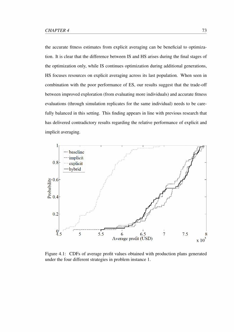
CHAPTER 4 73
the accurate fitness estimates from explicit averaging can be beneficial to optimiza-
tion. It is clear that the difference between IS and HS arises during the final stages of
the optimization only, while IS continues optimization during additional generations,
HS focuses resources on explicit averaging across its last population. When seen in
combination with the poor performance of ES, our results suggest that the trade-off
between improved exploration (from evaluating more individuals) and accurate fitness
evaluations (through simulation replicates for the same individual) needs to be care-
fully balanced in this setting. This finding appears in line with previous research that
has delivered contradictory results regarding the relative performance of explicit and
implicit averaging.
Figure 4.1: CDFs of average profit values obtained with production plans generatedunder the four different strategies in problem instance 1.
CHAPTER 4 74
Figure 4.2: CDFs of average profit values obtained with production plans generatedunder the four different strategies in problem instance 2.
4.7 Conclusion
Implicit averaging strategies reduce the impact of noise by having a sufficiently large
population, which ensures that individuals from promising regions of the search space
are sampled repeatedly (Jin and Branke, 2005; Syberfeldt et al., 2010). On the other
hand, explicit averaging strategies use average fitness values, obtained across a spe-
cific number of fitness evaluations, to ensure that evaluation of individuals is based on
fitness estimates that are more robust to noise (Jin and Branke, 2005).
One of the key findings of this study was that, in the context of our real-world prob-
lem, a noise-handling strategy based on explicit averaging did not provide a competi-
tive performance. More generally, this points to the fact that the computational costs
incurred by simulation replicates may be problematic in constrained time settings.
Furthermore, we found that implicit averaging performed robustly for both of the
CHAPTER 4 75
population sizes used. The performance of our hybrid strategy does indicate that some
effort towards explicit averaging may become important with increasing variability.
Under low levels of fitness variability, the hybrid strategy, implicit averaging and our
baseline showed a comparable performance. This situation changed with increasing
levels of fitness variability, when HS started to enhance overall performance.
Compared to a pure, implicit averaging strategy, the hybrid strategy misses out on
the last few generations of optimization. Our results show, however, that this disad-
vantage is more than counter-balanced by the benefits from an accurate final selection
step that reduces the likelihood of choosing an inferior individual (in terms of average
fitness) as the final solution.
4.8 Limitations and Future Research
The relevance of obtaining more reliable fitness estimates increases with the level of
variability, since there is a higher risk of choosing an inferior solution. It is, therefore,
intuitive that the final selection mechanism implemented in HS would be more bene-
ficial in such circumstances. But at the same time, the number of fitness evaluations
needed to obtain reliable estimates is expected to raise with higher fitness variabil-
ity, leaving to the evolutionary process a smaller share of the computational budget.
Therefore, further research may focus on investigating the right trade-off between ex-
ploration (IS) and accurate fitness evaluation (ES). In this sense, the application of
different sampling techniques (e.g. Latin Hypercube) during the final selection mecha-
nism might be worthy of future investigation, as it may allow a reduction in the number
of fitness evaluations required in this last step.
Our results underline issues around the computational cost of explicit averaging,
but also highlight that sporadic use of this strategy may, nevertheless, be beneficial.
In this study, the use of explicit averaging in the hybrid strategy was limited to the

CHAPTER 4 76
final selection step only. Future research may consider the possibility of using explicit
averaging at earlier points during the optimization process.
Chapter 5
Integrating Meta-Heuristics and Exact
Optimization Techniques (Manuscript
3)
J. E. Diaz, J. Handl, and D.-L. Xu. Integrating Meta-Heuristics, Simulation and Exact
Techniques for Production Planning of Failure-Prone Manufacturing Systems. Euro-
pean Journal of Operational Research, Submitted, 2015.
5.1 Abstract
In this chapter, we are concerned with the optimization of production plans in batch
manufacturing systems that include uncertainties, e.g. due to the possibility of produc-
tion line failures and uncertainty around repair times. In order to account for more re-
alistic situations, here we consider penalties imposed to deviations from a plan, which
is something that was not analysed in previous chapters. We also provide a general
formulation of this problem as an extended knapsack problem and describe a solution
approach based on SBO. Specifically, DES is used to model the existing uncertainty
77
CHAPTER 5 78
of the manufacturing process and to evaluate the average profit for any given produc-
tion plan. A GA is used to optimize across the space of possible production plans,
and we improve the algorithm’s optimization performance through the development
of specialized initialization operators that make use of mathematical programming in
combination with DES. We use our own GA implementation in order to have full
control of all parameters, something that was not possible with the default Matlab im-
plementation used in Chapter 3 and 4. The final models are benchmarked against ILP
and CCP within the context of a real-world production planning problem. We find
that our SBO approaches significantly outperform those exact optimization techniques
under the different levels of uncertainty analysed.
5.2 Introduction
The production planning process is an essential part of manufacturing strategy, since it
enables companies to achieve business objectives. In this study we address the produc-
tion planning problem of a real manufacturing company with insufficient capacity to
fully cover demand requirements. This company has to purchase the materials needed
for the next working month, before the beginning of the production period, and thus a
production plan for the following month must be available in order to make adequate
purchasing decisions. This is a difficult task because by the time a production plan
needs to be developed specific due dates of orders are still unknown and only demand
forecasts are available. Since due date information is not yet available during the spec-
ification of a production plan, scheduling decisions are not considered here (this is not
a scheduling problem).
Another feature of this system that further complicates the development of pro-
duction plans is the failure-prone nature of production lines. The occurrence of pro-
duction line failures reduces the total amount of products that can be manufactured
CHAPTER 5 79
and ultimately sold. Therefore, this company aims to develop production plans that
are not only profitable, but also plans that perform robustly under different realization
of breakdown events. Once a production plan has been decided and a failure occurs,
corrective actions cannot be implemented (at the operational level) without facing neg-
ative consequences. Here we try to incorporate those consequences into the problem
by penalizing any deviation from a production plan. Therefore, not only profitability
and system constraints have to be considered during the specification of a production
plan, but also the uncertainty around the occurrence of failures in production lines.
Given the uncertainty inherent to the system, addressing this problem through
mathematical programming approaches would require a number of assumptions that
may be overly stringent, and therefore, affect the validity of the resulting solutions (Ni-
kolopoulou and Ierapetritou, 2012; Gnoni et al., 2003). This is one of the reasons why
obtaining production plans under realistic assumptions has been a difficult challenge
for manufacturing companies. Overcoming this challenge is essential, especially in
the context of failure-prone manufacturing systems, where the occurrence of failures
in production lines can compromise the development of a production plan. Ignor-
ing the presence of uncertainty and including oversimplifying assumptions during the
problem formulation will inevitably lead to performance levels that deviate from the
original plan (Goh and Tan, 2009, 190). The degree of those deviations will mainly
depend on the levels of uncertainty present in the system or/and on the appropriateness
of the assumptions made.
In such cases, SBO is an interesting alternative because complex system features
can be explicitly and accurately incorporated into the problem via simulation (i.e. not
requiring a closed-form formulation), while an optimizer tries to find near-optimal
solutions. Therefore, in this study we present an effective SBO approach that com-
bines DES together with a meta-heuristic optimizer. Through this approach it is pos-
sible to incorporate via DES the uncertainty derived from production line failures,
CHAPTER 5 80
while optimization is performed by a GA. The optimization performance of this GA is
boosted by specialized initialization operators that combine DES, deterministic ILP
and CCP (Charnes and Cooper, 1959) in a variety of ways, as described in Sec-
tion 5.5.2. We demonstrate that our approach is able to generate better solutions to
the real-world problem analysed than the ones obtained via separate application of
meta-heuristics or mathematical optimization.
The remainder of this chapter is organized as follows: a review of relevant literature
and the contributions of this chapter are presented in Section 5.3. In Section 5.4, we
provide a general formulation of the problem analysed as an extended knapsack prob-
lem in order to demonstrate the wider applicability of our approach. In Section 5.5,
we describe a solution approach based on SBO. We also introduce a repair operator
which tries to fix unfeasible solutions generated during the optimization as well as two
specialized initialization operators which use a combination of mathematical program-
ming techniques (ILP and CCP) and DES to boost the optimization performance of the
SBO model. In Section 5.6, we address a real-world production planning problem of
a failure-prone manufacturing system to benchmark our models against ILP, CCP and
SBO without specialized initialization operators. Finally, conclusions derived from
this study, limitations and future research directions are given in Sections 5.7 and 5.8,
respectively.
5.3 Literature Review
The majority of studies in the existing literature on production planning of failure-
prone manufacturing systems are focused on finding optimal solutions through math-
ematical programming approaches. Those approaches; however, usually address ide-
alized cases where optimality conditions can be satisfied. For instance, Kouedeu et al.
(2014a) presented a hierarchical approach to determine production rates along with
CHAPTER 5 81
corrective and preventive maintenance policies. They aimed to minimize the dis-
counted overall cost of a system that manufactures a single product in a single ma-
chine, subject to random failures and that deteriorates with the number of failures.
Kouedeu et al. (2014b) formulated stochastic dynamic programming equations to de-
termine production rates for a single product manufactured by two machines, one with
production-dependent failure rates and the other with constant failure rates, with the
aim of minimizing inventory and shortage costs over an infinite time horizon. In a very
similar study, Kouedeu et al. (2014c) applied the same approach presented in Kouedeu
et al. (2014b) to minimize the discounted overall cost by specifying production rates
for a manufacturing and for a re-manufacturing machine that produce a single prod-
uct. Shi et al. (2014) proposed a discrete Markovian production model to determine, at
every customer arrival, the production rate and selling price (low or high) of a single
product manufactured by an unreliable machine, based on its inventory level.
Identifying a global optimal solution for real-world problems may often be unre-
alistic, due to the inherent complexity and uncertainty of real systems (Lacksonen,
2001), and thus practitioners are often satisfied with a good (but not necessarily op-
timal) solution that can be implemented in practice (Blum and Roli, 2008). This has
motivated the use of meta-heuristics in this area. For instance, Dahane et al. (2012)
addressed a multi-period multi-product (MPMP) production planning problem where
in each period a single machine, with production-dependent failure rate, first manu-
factures a product covering strategic demand and then a second product covering sec-
ondary demand. The authors applied a GA to simultaneously determine the production
rate of the first product as well as the duration of the production interval allocated in
each period to the manufacturing of the second product, in order to maximize the total
expected profit.
Another interesting alternative for this area is SBO. A smaller proportion of liter-
ature in this area has applied simulation in combination with optimization methods to
CHAPTER 5 82
find (near-optimal) solutions to more complex cases. For instance, Kenne and Gharbi
(2001) employed a combination of stochastic optimal control theory, DES, experimen-
tal design and response surface methodology to determine near-optimal production
rates, for a multi-product manufacturing system with parallel machines subject to fail-
ures and repairs, that minimize the expected discounted cost of inventory/backlog over
an infinite time horizon. Kenne and Gharbi (2004) determined near-optimal produc-
tion and machine repair rates of a multi-product and multi-machine manufacturing
system by applying the method proposed in Kenne and Gharbi (2001). Kenne and
Gharbi (2004) and Kenne and Gharbi (2001) are two papers where DES was used to
represent machine failures and repairs, and where the application of simulation in com-
bination with optimization enabled the analysis of more complex situations. Sel and
Bilgen (2014) iteratively applied mixed integer programming (MIP) based “Fix and
Optimize” heuristic to determine production and distribution plans and then used DES
to adjust capacities of production lines.
5.3.1 Simulation-based optimization
Over the past few decades, there has been a dramatic increase in the number of stud-
ies applying SBO to address different real-world problems (Korytkowski et al., 2013).
Studies applying a combination of simulation and mathematical programming are very
popular in the existing literature. For instance, Byrne and Bakir (1999) proposed a hy-
brid approach that combined LP and simulation to iteratively adjust the right-hand side
(RHS) of capacity constrains in order to obtain feasible solutions for a MPMP produc-
tion problem. Hung and Leachman (1996) applied a similar approach, but to modify
the left-hand side of capacity constraints of a semiconductor manufacturing system,
based on the results for production flow times obtained via DES. Kim and Kim (2001)
CHAPTER 5 83
combined the two former approaches to determine both, the amount of total work-
load per machine as well as the actual machine capacity utilized by the production
plan in each period. Byrne and Hossain (2005) incorporated the unit load concept
into the model proposed by Kim and Kim (2001) to make it suitable for just in time
production (Monden, 2011, p. 8). Lee and Kim (2002) and Safaei et al. (2010) used
a combination of mixed ILP (MILP) and simulation to address a multi-site MPMP
production and distribution planning problem. Almeder et al. (2009) tried to obtain
robust production, stocking and transportation plans to support supply chain decisions
at the operational level by applying a combination of DES and MILP. Ehrenberg and
Zimmermann (2012) presented an approach where input parameters of a MILP model
are specified iteratively via DES, to determine the scheduling of a make-to-order man-
ufacturing system. Arakawa et al. (2003) successfully solved a job shop scheduling
problem by implementing an optimization oriented method combined with simula-
tion. Monostori et al. (2010) applied a branch and cut algorithm to find solutions to
a medium-term production planning problem and to a short-term scheduling problem,
and then used DES to assess the sensitivity of the deterministic production schedules
and improve their robustness by supporting re-scheduling decisions.
Meta-heuristics and simulation techniques have also been combined, but to address
more complex problems where assumptions needed by mathematical programming
approaches cannot be satisfied. For instance, Kampf and Kochel (2006) combined a
GA with an event-oriented simulation model to determine sequencing and lot-sizing
rules for a multi-item production system with limited storage capacity. Li et al. (2009)
used a simulation model together with a cell evaluated GA to optimize resource al-
location, inventory and production policies for a dedicated re-manufacturing system.
Merkuryeva et al. (2010) combined stochastic simulation and multi-objective Pareto-
based GA together with response surface method-based linear search to determine cy-
cles and order-up-to levels of cyclic planning policies in multi-echelon supply chains.
CHAPTER 5 84
Gansterer et al. (2014) investigated different SBO approaches to determine appropriate
settings for planned leadtime, safety stock and lotsizing in a make-to-order environ-
ment, and concluded that a combination of DES with optimization procedures using
variable neighbourhood search provided better results than other SBO approaches anal-
ysed. Taleizadeh et al. (2013) proposed a combination of fuzzy simulation and a GA
to solve a multi-period inventory control problem with stochastic replenishment and
stochastic period length, for multiple products with limited storage and fuzzy customer
demand and showed that this method outperformed a combination of fuzzy simulation
and simulated annealing. Almeder and Hartl (2013) used a DES model as objective
function and proposed a variable neighbourhood search-based solution approach for
an off-line stochastic flexible flow-shop problem with limited buffers. Hong et al.
(2013) proposed a SBO method that combined continuous and discrete simulation with
simulated annealing and meta-models to find optimal design configurations. In their
approach the meta-models reduced the search space by providing good initial solu-
tions and then the meta-heuristic optimizer tried to improve those solutions towards
the optimum. Kose et al. (2015) presented a SBO approach where three meta-heuristic
optimizers (binary GA, binary-simulated annealing and binary-tabu search) were inte-
grated with a simulation model to solve a buffer allocation problem in a heat exchanger
production plant.
More specifically, the integration of DES and GAs has been successfully deployed
in several areas. For instance, Azzaro-Pantel et al. (1998) achieved efficiency im-
provements of a multi-purpose, multi-objective plant with limited storage. The authors
applied DES and a GA to accurately model the dynamic behaviour of the production
system and to solve the scheduling problem, respectively. It has also been applied to
determine robust design parameters as presented by Al-Aomar (2006). In order to en-
hance the selection scheme, the author incorporated Taguchis’s robustness measures
into the GA. The integration of DES and GAs has also been deployed to address other
CHAPTER 5 85
problems such as the one presented by Ding et al. (2005), where the uncertainty in-
volved in the supplier selection process was captured via DES and a GA was used to
optimize the supplier portfolio. Cheng and Yan (2009) applied an integration of DES
and a messy GA to determine the near optimal combination of resources in order to
enhance the performance of construction operations. This approach enabled the au-
thors to cope with the complexity and large dimensionality of the problem. Wu et al.
(2011) integrated DES with a GA to determine the order point for different product
types of a cross-docking center in order to minimize total cost. Through this approach
the solution space was efficiently reduced and more simulation effort was allocated to
promising regions via smart computing budget allocation. Korytkowski et al. (2013)
proposed an evolutionary simulation-based heuristics, where DES and a GA were de-
ployed to find near optimal solutions for dispatching rules allocation. The sequence
of orders determined through this approach improved the performance of a complex
multi-stage, multi-product manufacturing system.
The success of SBO approaches in addressing complex real-world problems moti-
vates us to develop a SBO approach to tackle the production planning problem anal-
ysed in this study. However, rather than combining simulation with a single optimiza-
tion technique, here we also take advantage of mathematical programming to enhance
the performance of our meta-heuristic optimizer, namely a GA. Thus in this chapter,
we highlight the synergies resulting from the integration of simulation techniques with
what could be seen as a matheuristic (Villegas et al., 2013; Boschetti et al., 2009)
optimizer. We test this approach in the context of a real-world production planning
problem, for which we provide a general formulation. We account for the uncertainty
in the problem via simulation and use the simulation model as our solution evaluation.
We use DES as our simulation technique due to its ability to incorporate stochastic
events (Riley, 2013) and to represent functional relationships between variables that are
not explicitly known or for which no analytical formulation exists (Steponavice et al.,
CHAPTER 5 86
2014). As mentioned above, meta-heuristics have been applied to stochastic problems
where the solution evaluation is performed via simulation (across multiple replications)
and are commonly used as optimizers in DES software (Figueira and Almada-Lobo,
2014). The ability of GAs to find near-optimal solutions in large, complex and discrete
solution spaces as well as their robust performance under noisy conditions reported
in previous studies (Mitchell, 1998; Baum et al., 1995), especially in optimization of
DES (Lacksonen, 2001), motivate us to use a GA as our optimizer, although a different
choice of meta-heuristic would also be suitable.
5.3.2 Contributions
The contributions of this chapter are the following: (i) we introduce a generaliza-
tion of a real-world production planning problem as a form of knapsack problem, (ii)
we propose two SBO approaches able to address that problem and (iii) demonstrate
their effectiveness under different uncertainty levels through a benchmark analysis
performed against ILP and CCP. However, we do not only provide evidence of the
poor performance of both exact optimization techniques, (iv) but more importantly we
demonstrate that ILP and CCP can be used to significantly improve the optimization
performance of our SBO approach. More specifically, we illustrate that the implemen-
tation of specialized initialization operators that draw upon the solutions returned by
ILP and CCP combined with DES in a variety of ways is able to significantly improve
the optimization performance of a standard GA. In general, this chapter highlights the
synergies resulting from the combination of simulation, mathematical programming
and meta-heuristic methods.
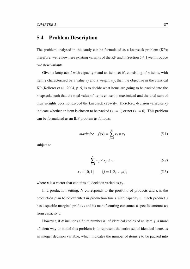
CHAPTER 5 87
5.4 Problem Description
The problem analysed in this study can be formulated as a knapsack problem (KP);
therefore, we review here existing variants of the KP and in Section 5.4.1 we introduce
two new variants.
Given a knapsack l with capacity c and an item set N, consisting of n items, with
item j characterized by a value v j and a weight w j, then the objective in the classical
KP (Kellerer et al., 2004, p. 5) is to decide what items are going to be packed into the
knapsack, such that the total value of items chosen is maximized and the total sum of
their weights does not exceed the knapsack capacity. Therefore, decision variables x j
indicate whether an item is chosen to be packed (x j = 1) or not (x j = 0). This problem
can be formulated as an ILP problem as follows:
maximize f (x) =n
∑j=1
v j× x j (5.1)
subject to
n
∑j=1
w j× x j ≤ c, (5.2)
x j ∈ 0,1 ( j = 1,2, . . . ,n), (5.3)
where x is a vector that contains all decision variables x j.
In a production setting, N corresponds to the portfolio of products and x is the
production plan to be executed in production line l with capacity c. Each product j
has a specific marginal profit v j and its manufacturing consumes a specific amount w j
from capacity c.
However, if N includes a finite number b j of identical copies of an item j, a more
efficient way to model this problem is to represent the entire set of identical items as
an integer decision variable, which indicates the number of items j to be packed into
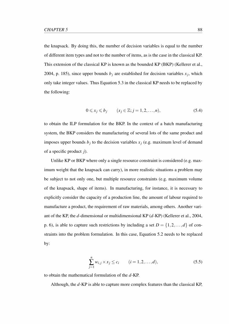
CHAPTER 5 88
the knapsack. By doing this, the number of decision variables is equal to the number
of different item types and not to the number of items, as is the case in the classical KP.
This extension of the classical KP is known as the bounded KP (BKP) (Kellerer et al.,
2004, p. 185), since upper bounds b j are established for decision variables x j, which
only take integer values. Thus Equation 5.3 in the classical KP needs to be replaced by
the following:
0 6 x j 6 b j (x j ∈ Z; j = 1,2, . . . ,n), (5.4)
to obtain the ILP formulation for the BKP. In the context of a batch manufacturing
system, the BKP considers the manufacturing of several lots of the same product and
imposes upper bounds b j to the decision variables x j (e.g. maximum level of demand
of a specific product j).
Unlike KP or BKP where only a single resource constraint is considered (e.g. max-
imum weight that the knapsack can carry), in more realistic situations a problem may
be subject to not only one, but multiple resource constraints (e.g. maximum volume
of the knapsack, shape of items). In manufacturing, for instance, it is necessary to
explicitly consider the capacity of a production line, the amount of labour required to
manufacture a product, the requirement of raw materials, among others. Another vari-
ant of the KP, the d-dimensional or multidimensional KP (d-KP) (Kellerer et al., 2004,
p. 6), is able to capture such restrictions by including a set D = 1,2, . . . ,d of con-
straints into the problem formulation. In this case, Equation 5.2 needs to be replaced
by:
n
∑j=1
wi, j× x j ≤ ci (i = 1,2, . . . ,d), (5.5)
to obtain the mathematical formulation of the d-KP.
Although, the d-KP is able to capture more complex features than the classical KP,
CHAPTER 5 89
it is still unable to model the situation when multiple knapsacks are available. When a
KP includes a set M = 1,2, . . . ,m of knapsacks, where each knapsack l has a given
capacity cl , and every product j has to be packed at most into one knapsack, it is
known as the multiple knapsack problem (MKP) (Kellerer et al., 2004, p. 7). When
only a subset A j ⊆ M of knapsacks can hold a specific item j, then this problem is
referred to as the MKP with assignment restrictions (MKAR) (Dawande et al., 2000).
In a manufacturing context, MKAR extends the MKP to the situation where multiple
production lines are available and where each production line is able to produce only
certain products. The mathematical formulation of the MKAR is as follows:
maximize f (x) =n
∑j=1
∑l∈A j
v j× xl, j (5.6)
subject to
n
∑j=1
w j× xl, j ≤ cl (l = 1,2, . . . ,m), (5.7)
∑l∈A j
xl, j ≤ 1 ( j = 1,2, . . . ,n), (5.8)
xl, j ∈ 0,1 (l ∈ A j; j = 1,2, . . . ,n). (5.9)
5.4.1 New Variants of the KP Problem: d-MBKAR and d-MBKARS
In this section we introduce a deterministic and a stochastic variant of the KP to define
a more general class of problem that can be tackled with our approach. Both vari-
ants generalize features of a real-world production planning problem of a failure-prone
batch manufacturing system, whose details are presented in Chapter 2. In both variants
CHAPTER 5 90
we relax Equation 5.8, so that several identical copies of item j can be packed into dif-
ferent knapsacks. Moreover, instead of binary decision variables, integer variables are
used to represent the number of units of item j to be packed into a specific knapsack l.
We also set upper bounds b j for the total number of copies of item j packed across all
knapsacks (Equation 5.12). Furthermore, we eliminate the general assumption (made
in KPs to avoid trivial situations (Kellerer et al., 2004, p. 10)) that v j, wi, j and ci can
take only positive values, for it precludes the consideration of more complex features
present in real-world problems such as the case of complementary items. In this case,
complementary items must be packed across knapsacks in a specific proportion to de-
rive value from them. For instance, in manufacturing systems, it is common that some
products are employed (in a certain proportion) as raw materials during the manufac-
turing of another product. Representing these constraints in the form of Equation 5.11
requires that: (i) v j can take negative values to represent the marginal cost of products
used as raw materials, (ii) wi, j can take negative values to represent the yield (per lot)
of product j in production line l and positive values to represent the amount of raw
materials needed to manufacture one lot of product j and (iii) ci can be equal to zero.
The ILP formulation of such problem is the following:
maximize f (x) =n
∑j=1
∑l∈A j
v j× xl, j (5.10)
subject to
n
∑j=1
∑l∈A j
wi, j× xl, j ≤ ci (i = 1,2, . . . ,d), (5.11)
∑l∈A j
xl, j 6 b j (xl, j ∈ Z≥0; j = 1,2, . . . ,n). (5.12)
We refer to this deterministic variant of the KP as the multidimensional multiple
CHAPTER 5 91
bounded knapsack problem with assignment restrictions (d-MBKAR).
However, reality is not deterministic, and thus a stochastic version of the d-MBKAR
problem (d-MBKARS) is needed. In the d-MBKARS we consider that knapsacks are
subject to random failures during the packing process. Here, uncertainty is incor-
porated into the problem by considering the reduction in capacity caused by knapsack
failures. Therefore, given a packing plan x, the actual number of units of item j packed
into knapsack l at the end of the packing process, denoted here by sl, j, depends on the
number of failures that have occurred during the packing process and on the capacity
reduction caused by the corresponding repairs. Moreover, we assume that any devia-
tion from the packing plan x is subject to a penalty (k j) proportional to that deviation,
i.e. k j× (xl, j− sl, j), and thus uncertainty needs to be carefully considered during the
specification of a packing plan.
The realization of a packing plan, denoted as s (vector that contains all sl, j), is
obtained here via simulation due to the difficulty of finding a closed-form expression
able to map a packing plan x onto its realization s. In this sense, the simulation model
can be seen here as the function g(x) that enables us to perform such mapping without
the requirement of a closed-form expression. Other parameters such as price volatility,
demand fluctuations and variability in production yields could also be incorporated
into the problem by modelling them via simulation.
The occurrence of a knapsack failure during the packing process of an item is
modelled by a random variable Hl , whose numerical values hl are sampled (every
time an item needs to be packed into a knapsack) from a PMF with sample space
ΩH = 0,1. hl = 1 represents the occurrence of a failure, whereas hl = 0 indicates that
no failure occurred. The probability that hl = 1 is pHl(1) = pl; consequently, pHl(0) =
1− pl . Here, pl is the probability that a knapsack fails during the packing process of
an item, and thus the number of knapsack failures depends on the number of items to
be loaded. After every knapsack failure, a repair service needs to be undertaken. The
CHAPTER 5 92
reduction in capacity λl caused by a repair service is the numerical realization of a
random variable Λl , modelled by an exponential PDF with known mean µl .
The formulation of the d-MBKARS is as follows:
maximize f (x) =n
∑j=1
∑l∈A j
v j× sl, j− k j× (xl, j− sl, j) (5.13)
subject to the set of constraints in the form of Equations 5.11 and 5.12.
Features of the d-MBKARS problem translated to a batch manufacturing system
could be represented by unreliable production lines that require a repair service after
one of its components stopped functioning properly. In this context, pl is the proba-
bility that a failure occurs in production line l during the manufacturing of a product
lot, and the delay λl caused by a repair service is equivalent to the capacity loss in the
d-MBKARS problem. The reduction in capacity caused by production line failures
has the effect that a production plan cannot be fully realized, which means that some
products will not be produced on time. Deviations from the original plan may have se-
rious consequences not only on the company’s profitability, but also on its image and
reputation. Here, we only consider consequences that can be quantified by a penalty
proportional to that deviation.
Note that the RHS of Equation 5.11 is a constant, even with ci related to design
(theoretical) knapsack capacities (Heizer et al., 2004, p. 252). Therefore, a packing
plan x that is feasible according to the set of constraints in the form of Equations 5.11
and 5.12 might not always be realized in the d-MBKARS problem. In other words, xl, j
is not always equal to sl, j in the d-MBKARS because the former is a number, whereas
the latter is the numerical value of the random variable Sl, j.
Although, BKP (Pisinger, 2000), d-KP (Chen and Hao, 2014; Balev et al., 2008;
Wilbaut et al., 2009), MKP (Garcia-Martinez et al., 2014; Yamada and Takeoka, 2009;
Kataoka and Yamada, 2014), MKAR (Dawande et al., 2000) and different stochastic
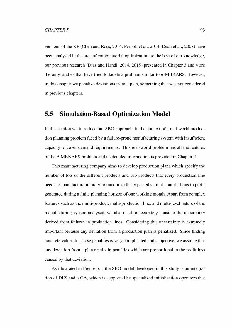
CHAPTER 5 93
versions of the KP (Chen and Ross, 2014; Perboli et al., 2014; Dean et al., 2008) have
been analysed in the area of combinatorial optimization, to the best of our knowledge,
our previous research (Diaz and Handl, 2014, 2015) presented in Chapter 3 and 4 are
the only studies that have tried to tackle a problem similar to d-MBKARS. However,
in this chapter we penalize deviations from a plan, something that was not considered
in previous chapters.
5.5 Simulation-Based Optimization Model
In this section we introduce our SBO approach, in the context of a real-world produc-
tion planning problem faced by a failure-prone manufacturing system with insufficient
capacity to cover demand requirements. This real-world problem has all the features
of the d-MBKARS problem and its detailed information is provided in Chapter 2.
This manufacturing company aims to develop production plans which specify the
number of lots of the different products and sub-products that every production line
needs to manufacture in order to maximize the expected sum of contributions to profit
generated during a finite planning horizon of one working month. Apart from complex
features such as the multi-product, multi-production line, and multi-level nature of the
manufacturing system analysed, we also need to accurately consider the uncertainty
derived from failures in production lines. Considering this uncertainty is extremely
important because any deviation from a production plan is penalized. Since finding
concrete values for those penalties is very complicated and subjective, we assume that
any deviation from a plan results in penalties which are proportional to the profit loss
caused by that deviation.
As illustrated in Figure 5.1, the SBO model developed in this study is an integra-
tion of DES and a GA, which is supported by specialized initialization operators that
CHAPTER 5 94
combine DES with mathematical programming techniques (see Section 5.5.2). Ac-
cording to the taxonomy provided in Figueira and Almada-Lobo (2014), our model
would be classified as an “evaluation function - simulation-based iterations/discrete
heuristic-different - realizations for each solution” (EF-OSI/DH-DR1S) model, since
here optimization is performed by a meta-heuristic optimizer based exclusively on
fitness values computed with responses generated via simulation, across different real-
izations of integer solutions.
Problem GA’s initialization GA
DES
f (·)
ILP CCP DES Uncertainty
x s
f (x)
Figure 5.1: SBO model.
The DES model employed in this study corresponds to the one used in Chapter 4,
which is developed in SimEventsr (The MathWorks, Inc., 2014). It is responsible
for capturing the delays (λl) caused by failures in production lines and provides to
the GA information about the number of lots of a specific product j manufactured by
production line l, which is necessary to compute fitness values.
Since we need to search for a production plan that performs robustly under differ-
ent realizations of orders due dates, in the DES model the production sequence of a
production plan is randomly initialized for every production line, except for products
that are used as raw materials during the manufacturing of other products. In order to
assure the static logic of the model, products used as raw materials are manufactured
before any other product to be manufactured in the same production line.
CHAPTER 5 95
We developed in Matlabr R2014a’s (The MathWorks, Inc., 2014) a real-coded
GA, that employs uniform crossover (crossover probability: 1), Gaussian mutation
(mutation probability: 0.3, mutation fraction: 0.1, scale: 0.4 and shrink: 0.1), tour-
nament selection (tournament size: 2), a population size of 40 individuals, 50 gen-
erations and the final solution selection employs a computational budget (E) of 3000
fitness evaluations (see Section 5.5.1 for more details about E). Here, we used the irace
package (Lopez-Ibanez et al., 2011) to tune the parameters mentioned above, except
for population size, which was determined after extensive experimentation. Table 5.3
in Appendix 5.A presents the possible parameter values given to irace to search for
a tuned configuration for our GA. Those possible parameter values were chosen after
preliminary experiments and the final configuration of parameters was identified by
irace based on 300 experiments.
We implemented in this GA a truncation procedure that rounds each decision
variable after crossover and mutation, in order to ensure compliance with integer
constraints. We also implemented the constraint-handling method proposed by Deb
(2000). Elitism is incorporated into this GA by combining the entire parent and off-
spring populations, and then extracting from this combined population the best indi-
viduals, which will constitute the new population for the next generation. During this
extraction procedure and during tournament selection, feasible solutions are preferred
over unfeasible ones and are ranked according to their fitness values, whereas unfeasi-
ble solutions are ranked first according to the number of constraint violations and then
according to the magnitude of each violation (by how much a constraint was violated).
For this reason fitness is not computed for unfeasible solutions. All computations are
executed in parallel on a 16 core Intel(R) Xeon(R) CPU L5640 @ 2.27GHz with 24
GB of RAM running Scientific Linux, release 6.2.
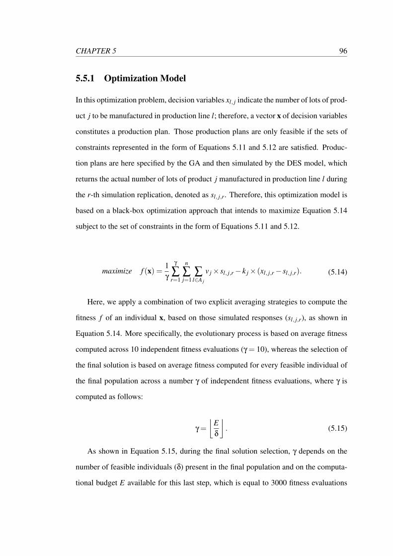
CHAPTER 5 96
5.5.1 Optimization Model
In this optimization problem, decision variables xl, j indicate the number of lots of prod-
uct j to be manufactured in production line l; therefore, a vector x of decision variables
constitutes a production plan. Those production plans are only feasible if the sets of
constraints represented in the form of Equations 5.11 and 5.12 are satisfied. Produc-
tion plans are here specified by the GA and then simulated by the DES model, which
returns the actual number of lots of product j manufactured in production line l during
the r-th simulation replication, denoted as sl, j,r. Therefore, this optimization model is
based on a black-box optimization approach that intends to maximize Equation 5.14
subject to the set of constraints in the form of Equations 5.11 and 5.12.
maximize f (x) =1γ
γ
∑r=1
n
∑j=1
∑l∈A j
v j× sl, j,r− k j× (xl, j,r− sl, j,r). (5.14)
Here, we apply a combination of two explicit averaging strategies to compute the
fitness f of an individual x, based on those simulated responses (sl, j,r), as shown in
Equation 5.14. More specifically, the evolutionary process is based on average fitness
computed across 10 independent fitness evaluations (γ = 10), whereas the selection of
the final solution is based on average fitness computed for every feasible individual of
the final population across a number γ of independent fitness evaluations, where γ is
computed as follows:
γ =
⌊Eδ
⌋. (5.15)
As shown in Equation 5.15, during the final solution selection, γ depends on the
number of feasible individuals (δ) present in the final population and on the computa-
tional budget E available for this last step, which is equal to 3000 fitness evaluations
CHAPTER 5 97
(E = 3000). We used the irace package to determine the computational budget allo-
cated to the final solution selection.
Unlike in Chapter 4, where the optimization started with poor quality solutions
and a very limited computational budget was available, here high quality solutions are
created at the beginning of the optimization by specialized initialization operators (pre-
sented in Section 5.5.2). Therefore, we apply a modified version of the hybrid strategy
proposed in Chapter 4 in order to select individuals based on more reliable fitness es-
timates during the optimization. After extensive experimentation, we concluded that
using 10 fitness evaluations to compute average fitness during the evolutionary process
returned similar solutions in terms of quality compared to using a sample size of 30,
but at a much lower computational cost.
5.5.2 Initialization Operators
Exact and heuristic optimization techniques have been previously combined to take ad-
vantage of the synergies between those approaches. For instance, Gomes and Oliveira
(2006) solved irregular strip packing problems by applying LP to generate neighbour-
hoods, while simulated annealing guided the search over the solution space. Another
example is Reisi-Nafchi and Moslehi (2015), where the authors employed the rounded
solution returned by LP as one of the individuals of the GA’s initial population when
solving the two-agent order acceptance and scheduling problem. Here, we present two
different initialization operators to create part of the GA’s initial population. Solutions
created by the specialized initialization operators through DES or/and mathematical
programming techniques (as described in Sections 5.5.2.1 and 5.5.2.2) are refereed to
as ILP-derived solutions. Both initializations intend to boost the optimization perfor-
mance of the GA by including into the GA’s initial population feasible ILP-derived
CHAPTER 5 98
solutions with high quality alleles, which are likely to be part of a good quality solu-
tion. After extensive experimentation we could determine that given a population size
of 40, the incorporation of up to 4 ILP-derived solutions into the GA’s initial population
promoted the creation of new high quality solutions during the optimization process.
Our preliminary experiments revealed that the incorporation of more ILP-derived so-
lutions into the GA’s initial population had a detrimental effect on the diversity of the
initial population, which mainly led to premature convergence. Therefore, both ini-
tialization procedures incorporate into the GA’s initial population up to 4 ILP-derived
solutions and the rest of individuals are randomly initialized.
5.5.2.1 Initialization 1
Initialization 1 incorporates as part of the GA’s initial population the ILP solution (x∗)
for the d-MBKAR problem (optimize Equation 5.10 subject to constraints in the form
of Equations 5.11 and 5.12). This deterministic ILP solution is a feasible and optimal
solution for a fully reliable system. However, s deviates from x∗ when uncertainty is
present in the system (s 6= x∗). To capture those deviations we employ the DES model
to run one independent simulation of x∗ and obtain its simulated response s, which is
also included as part of the GA’s initial population.
Furthermore, the solution x′∗ obtained via CCP and one simulated response of x′∗
are also incorporated into the GA’s initial population. x′∗ is obtained by optimizing
Equation 5.10 subject to constraints in the form of Equation 5.12 and the following:
n
∑j=1
∑l∈A j
wi, j× xl, j ≤ ci (i = 1,2, . . . ,d−m), (5.16)
P( n
∑j=1
wl, j× xl, j ≤C′l)≥ αl (l = 1,2, . . . ,m), (5.17)
where d−m represents the number of constraints not related to capacities of production
CHAPTER 5 99
lines. All resource constraints are in the form of Equation 5.16, except for those related
to capacity of production lines, which are represented in the form of Equation 5.17. A
constraint formulated in the form of Equation 5.17 is a probabilistic constraint, as C′l is
a random variable with known PDF, which models the number of hours that production
line l is operative during a working month (24 days). This constraint restricts the
probability of infeasibility to be no greater than a specified threshold 1−αl , where
αl can take values between 0 and 1. In order to use an appropriate value for αl , we
computed CCP solutions with αl ∈ [0.95,0.99] and then we calculated average profit
values for each of those CCP solutions, across a sample of 5000 profit values (see
Section 5.6 for more details about the sample size chosen) obtained by simulating
each solution in the DES model. The CCP solution obtained with αl = 0.95 returned
the highest average profit under the three problem instances analysed (see Section 5.6
for more details about problem instances analysed); therefore, in this study x′∗ was
calculated with αl = 0.95.
If FC′lis CDF of C′l , then Equation 5.17 is equivalent to:
FC′l
( n
∑j=1
wl, j× xl, j
)≤ 1−αl ⇔
n
∑j=1
wl, j× xl, j ≤ F−1C′l
(1−αl
)(l = 1,2, . . . ,m).
(5.18)
This means that we first need to obtain the PDF of each C′l before applying an available
method to solve this problem (the reader is referred to Shapiro et al. (2014); Wallace
and Ziemba (2005); Kall and Wallace (1995) for details about CCP). We implemented
timers within the DES model in order to measure the exact number of hours that each
production line was operative during a working month, denoted here as c′l , and used the
DES model to generate 10000 numerical values of each C′l by simulating a production
plan that fully utilizes the design capacity of all production lines. Based on those
simulated responses (c′l) we fitted a PDF to each sample. We used a sample size of
CHAPTER 5 100
10000 numerical values of C′l because, under the highest uncertainty level analysed (see
Section 5.6 for details about problem instance 3), the same solution x′∗ was obtained
when PDFs of C′l were estimated based on a sample size of 10000 and 50000 c′l values.
Any production plan that fully utilizes the design capacity of all production lines can
be simulated to obtain numerical values of C′l , since pl is the probability that a failure
occurs in production line l during the manufacturing of a lot of any product. Here we
used a production plan where all its decision variables were equal to 72 lots, which is
the design capacity of the different production lines (see Chapter 2 for more details).
It is important to note that using the PDFs of C′l to model the uncertainty present in
the system is already a simplified version of the DES model because by doing that, the
occurrence of failures which are production-level dependent and the repair times are
not explicitly considered.
5.5.2.2 Initialization 2
In this initialization we use again the DES model to obtain numerical values of C′l by
simulating a production plan that fully utilizes the design capacity of all production
lines (see Initialization 1 for more details about that production plan), and then we use
those values (c′l) as the RHS of Equation 5.19:
n
∑j=1
wl, j× xl, j ≤ c′l (l = 1,2, . . . ,m). (5.19)
Here, 4 numerical values of each C′l are generated and for each set of c′l values an
ILP solution is found by optimizing Equation 5.10 subject to the sets of constraints
in the form of Equations 5.12, 5.16 and 5.19. In order to maintain diversity, dupli-
cates are eliminated among those 4 ILP solutions and then the remaining solutions are
incorporated into the GA’s initial population.
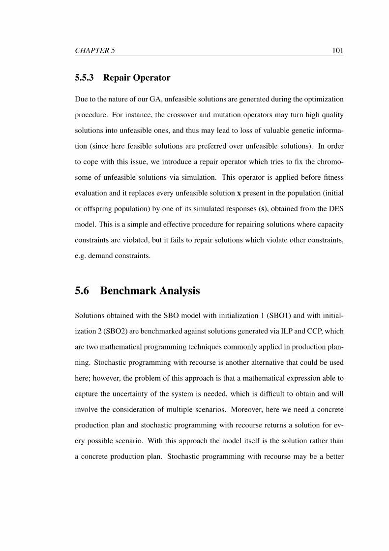
CHAPTER 5 101
5.5.3 Repair Operator
Due to the nature of our GA, unfeasible solutions are generated during the optimization
procedure. For instance, the crossover and mutation operators may turn high quality
solutions into unfeasible ones, and thus may lead to loss of valuable genetic informa-
tion (since here feasible solutions are preferred over unfeasible solutions). In order
to cope with this issue, we introduce a repair operator which tries to fix the chromo-
some of unfeasible solutions via simulation. This operator is applied before fitness
evaluation and it replaces every unfeasible solution x present in the population (initial
or offspring population) by one of its simulated responses (s), obtained from the DES
model. This is a simple and effective procedure for repairing solutions where capacity
constraints are violated, but it fails to repair solutions which violate other constraints,
e.g. demand constraints.
5.6 Benchmark Analysis
Solutions obtained with the SBO model with initialization 1 (SBO1) and with initial-
ization 2 (SBO2) are benchmarked against solutions generated via ILP and CCP, which
are two mathematical programming techniques commonly applied in production plan-
ning. Stochastic programming with recourse is another alternative that could be used
here; however, the problem of this approach is that a mathematical expression able to
capture the uncertainty of the system is needed, which is difficult to obtain and will
involve the consideration of multiple scenarios. Moreover, here we need a concrete
production plan and stochastic programming with recourse returns a solution for ev-
ery possible scenario. With this approach the model itself is the solution rather than
a concrete production plan. Stochastic programming with recourse may be a better
CHAPTER 5 102
alternative to make decisions at the operational level, namely to re-optimize a produc-
tion plan after the occurrence of failures; however, this is outside of the scope of this
study. Additionally, we benchmark SBO1 and SBO2 against the SBO model without
any of the two initialization operators (SBO3). Here, our intention is not only to com-
pare those different strategies, but more importantly, we are interested in understanding
how they perform relative to each other and how performance differences evolve with
increasing uncertainty levels, so we can get a clearer idea about what method is more
appropriate under different circumstances.
Three problem instances are addressed here to evaluate the models mentioned un-
der different levels of uncertainty. Table 5.1 presents the probabilities pl that a failure
occurs during the manufacturing of a product lot in the different production lines per
problem instance, as well as the parameter µl of the exponential PDFs used to model
the random variables Λl , whose numerical values represent the delay caused per repair
service of a production line. Please note that pl values in instance 1 as well as µl val-
ues are based on historical data collected over a period of 54 months. As mentioned
in Chapter 2, pl values in instance 1 are conservative (too optimistic) lower bounds for
such probabilities, since they were calculated based on the number of production line
failures recorded and assuming that every production line remained operative and was
fully utilized during a period of 54 months (number of months for which information is
available), which is an unrealistic assumption; therefore, pl values in problem instance
2 and 3 are the double and triple, respectively, of the corresponding pl values in prob-
lem instance 1. Only production line 2, 3 and 4 have been assigned with a positive pl
because failures in the other lines rarely or never occurred, according to the historical
information provided by the company (see Table 2.5 in Chapter 2).
SBO1, SBO2 and SBO3 are executed 30 times using different seeds for the random
number generator in every run. Average profit values, measured in United States Dollar
(USD), are computed across a sample of 5000 profit values obtained via stochastic
CHAPTER 5 103
Instance 1 Instance 2 Instance 3 Instance 1, 2 and 3Production
pl pl plΛl
line (l) PDF µl (d)1 0.0000 0.0000 0.0000 — —2 0.0355 0.0710 0.1065 Exponential 2.033 0.0468 0.0936 0.1404 Exponential 2.244 0.0471 0.0942 0.1413 Exponential 3.215 0.0000 0.0000 0.0000 — —6 0.0000 0.0000 0.0000 — —7 0.0000 0.0000 0.0000 — —
Table 5.1: pl per problem instance and PDFs specifications to model Λl .
simulation for every final solution of each run performed with SBO1, SBO2 and SBO3.
A sample size of 5000 profit values was chosen because it returned estimates that
were reliable enough for the purpose of our analysis, given that the relative change
of average profit computed across samples of 10000 and 5000 profit values in the
problem instance with highest uncertainty level (problem instance 3) was lower than
1e−2. Additionally, 30 average profit values of the solutions obtained with ILP (x∗) and
with CCP (x′∗) are also computed across a sample size of 5000 profit values obtained
with those solutions via stochastic simulation. Those average profit values are used to
evaluate the optimization performance of the different models.
5.6.1 Results
Under all uncertainty levels analysed, SBO1 and SBO2 were able to generate produc-
tion plans that outperformed in terms of average profitability the solutions given by
ILP, CCP and SBO3. This is according to results from Mann-Whitney U tests (Mann
and Whitney, 1947) presented in Tables 5.4a, 5.4b and 5.4c (Appendix 5.B), which sta-
tistically show that the average profit values obtained with x∗, x′∗ and with production
plans given by SBO3 are stochastically smaller (p < .01) than the ones obtained with
solutions given by SBO1 and SBO2, in all problem instances. The advantage of SBO1
CHAPTER 5 104
and SBO2 over ILP, CCP and SBO3 under the uncertainty levels analysed is also il-
lustrated in Figures 5.2, 5.3 and 5.4, where the CDFs of average profits generated with
x∗, x′∗ and with production plans given by SBO3 are dominated (first-order stochastic
dominance (Hadar and Russell, 1969)) by the CDFs of average profit values obtained
with solutions given by SBO1 and SBO2.
Under low uncertainty levels (problem instance 1), the optimization performance
of SBO1 and SBO2 did not evidence a significant (p > .05) difference. However, un-
der medium and high uncertainty levels (problem instance 2 and 3) SBO1 was clearly
outperformed by SBO2. This is confirmed by results from Mann-Whitney U tests
presented in Tables 5.4a, 5.4b and 5.4c (Appendix 5.B), and are also illustrated in Fig-
ures 5.2, 5.3 and 5.4. These results demonstrate that SBO2 is a more effective strategy
than SBO1 under increasing uncertainty levels. This is because initialization 2 draws
upon simulation responses for the RHSs of capacity constraints (c′l) to return solutions
created according to the level of uncertainty captured by those RHSs, whereas in ini-
tialization 1 uncertainty is simply captured by incorporating x′∗ into the GA’s initial
population as well as the simulated responses (s) of x∗ and x′∗.
Moreover, both specialized initialization operators significantly (p< .01) improved
the optimization performance of the SBO model under all uncertainty levels analysed,
as shown in Tables 5.4a, 5.4b and 5.4c (Appendix 5.B). This is also illustrated in Fig-
ures 5.2, 5.3 and 5.4, where the CDFs of average profits generated with production
plans given by SBO3 are dominated (first-order stochastic dominance) by the CDFs
of average profit values obtained with solutions given by SBO1 and SBO2. We exe-
cuted 30 additional runs of SBO3 in every problem instance, but this time we allocated
100 rather than 50 generations to the optimization procedure of SBO3 (SBO3x2) in
order to investigate whether the performance gap between SBO models with and with-
out specialized initialization operators decreases or not when a bigger computational
budget is available. Our results suggest that SBO1 and SBO2 outperform SBO3 even
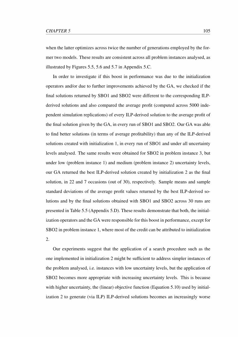
CHAPTER 5 105
when the latter optimizes across twice the number of generations employed by the for-
mer two models. These results are consistent across all problem instances analysed, as
illustrated by Figures 5.5, 5.6 and 5.7 in Appendix 5.C.
In order to investigate if this boost in performance was due to the initialization
operators and/or due to further improvements achieved by the GA, we checked if the
final solutions returned by SBO1 and SBO2 were different to the corresponding ILP-
derived solutions and also compared the average profit (computed across 5000 inde-
pendent simulation replications) of every ILP-derived solution to the average profit of
the final solution given by the GA, in every run of SBO1 and SBO2. Our GA was able
to find better solutions (in terms of average profitability) than any of the ILP-derived
solutions created with initialization 1, in every run of SBO1 and under all uncertainty
levels analysed. The same results were obtained for SBO2 in problem instance 3, but
under low (problem instance 1) and medium (problem instance 2) uncertainty levels,
our GA returned the best ILP-derived solution created by initialization 2 as the final
solution, in 22 and 7 occasions (out of 30), respectively. Sample means and sample
standard deviations of the average profit values returned by the best ILP-derived so-
lutions and by the final solutions obtained with SBO1 and SBO2 across 30 runs are
presented in Table 5.5 (Appendix 5.D). These results demonstrate that both, the initial-
ization operators and the GA were responsible for this boost in performance, except for
SBO2 in problem instance 1, where most of the credit can be attributed to initialization
2.
Our experiments suggest that the application of a search procedure such as the
one implemented in initialization 2 might be sufficient to address simpler instances of
the problem analysed, i.e. instances with low uncertainty levels, but the application of
SBO2 becomes more appropriate with increasing uncertainty levels. This is because
with higher uncertainty, the (linear) objective function (Equation 5.10) used by initial-
ization 2 to generate (via ILP) ILP-derived solutions becomes an increasingly worse
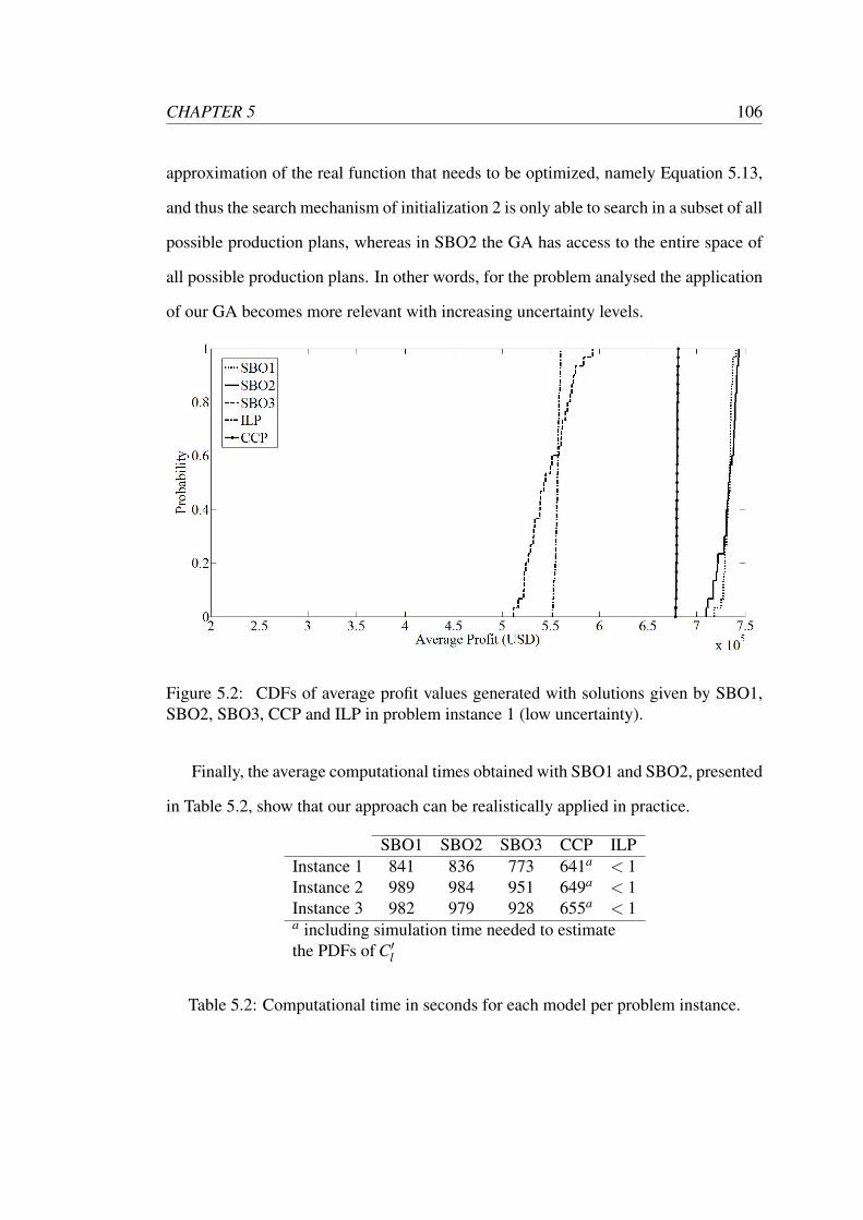
CHAPTER 5 106
approximation of the real function that needs to be optimized, namely Equation 5.13,
and thus the search mechanism of initialization 2 is only able to search in a subset of all
possible production plans, whereas in SBO2 the GA has access to the entire space of
all possible production plans. In other words, for the problem analysed the application
of our GA becomes more relevant with increasing uncertainty levels.
Figure 5.2: CDFs of average profit values generated with solutions given by SBO1,SBO2, SBO3, CCP and ILP in problem instance 1 (low uncertainty).
Finally, the average computational times obtained with SBO1 and SBO2, presented
in Table 5.2, show that our approach can be realistically applied in practice.
SBO1 SBO2 SBO3 CCP ILPInstance 1 841 836 773 641a < 1Instance 2 989 984 951 649a < 1Instance 3 982 979 928 655a < 1a including simulation time needed to estimatethe PDFs of C′l
Table 5.2: Computational time in seconds for each model per problem instance.
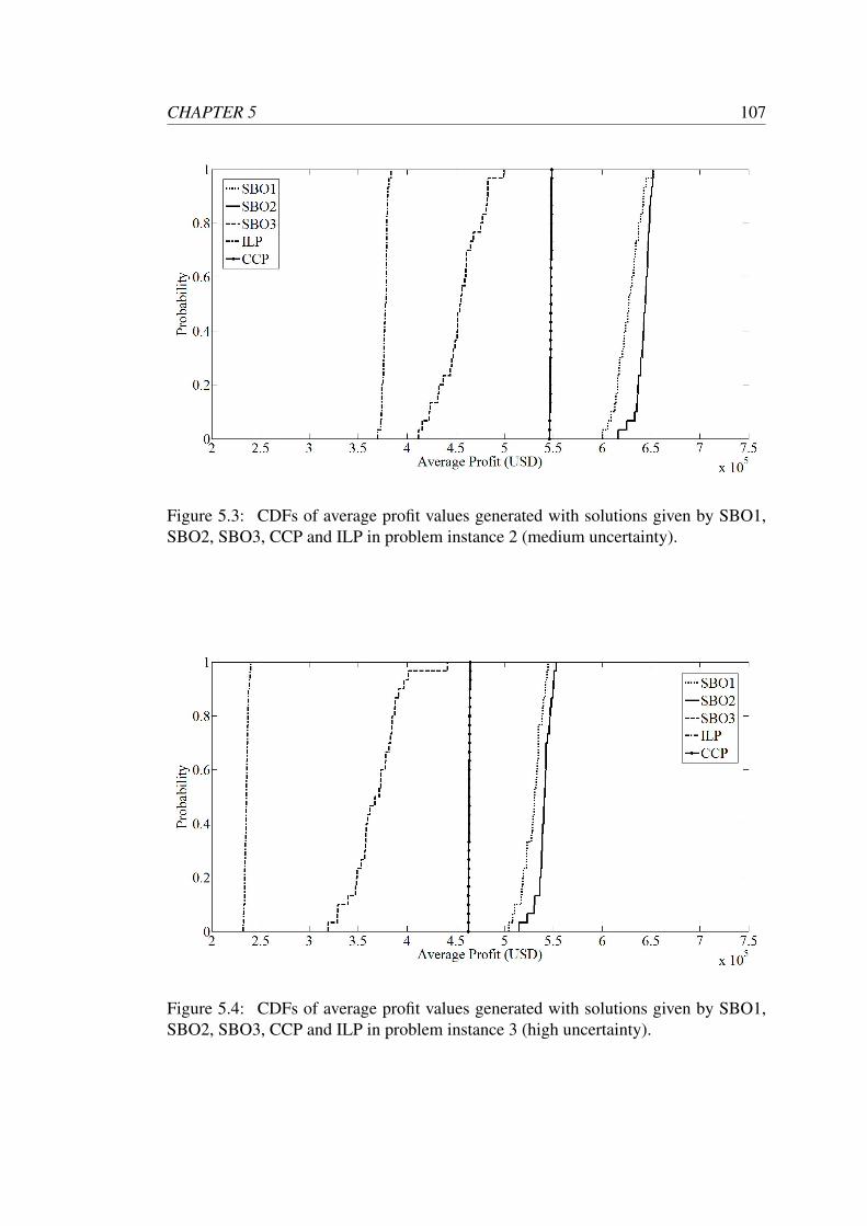
CHAPTER 5 107
Figure 5.3: CDFs of average profit values generated with solutions given by SBO1,SBO2, SBO3, CCP and ILP in problem instance 2 (medium uncertainty).
Figure 5.4: CDFs of average profit values generated with solutions given by SBO1,SBO2, SBO3, CCP and ILP in problem instance 3 (high uncertainty).
CHAPTER 5 108
5.7 Conclusion
Our experiments illustrate how the performance of deterministic and stochastic global
optimal solutions, obtained under overly stringent assumptions, deviates from the opti-
mum in the presence of uncertainty. This finding is in accordance with results reported
by Wang et al. (2015), where the optimal solution for a deterministic travelling sales-
man problem (TSP) evidenced a poor performance in a TSP under uncertainty.
Our results also show, as may be expected, that an accurate incorporation of the
existing uncertainty into the problem formulation becomes more important with in-
creasing uncertainty levels. In this sense, it is worth emphasizing that our SBO ap-
proach explicitly models (via simulation) the key features that bring uncertainty to the
problem, namely the occurrence of failures that are production-level dependent and
the delays caused by the corresponding repair services. CCP, on the other hand, loses
information on those key features that we are interested in capturing, since it tries to
model that uncertainty by using PDFs (which need to be estimated via simulation) of
the RHSs of the capacity constraints (C′l). Furthermore, here CCP has no mechanism
to consider penalties imposed to deviations from a plan during the specification of a
production plan, which is something that can be explicitly considered in our SBO ap-
proach. In this sense, our approach is able to adjust a production plan according to
the penalty level, whereas the production plan obtained with CCP is the same under
different penalty levels.
We also demonstrate how the combined use of simulation (DES) and mathematical
programming techniques (ILP and CCP) to specify part of the GA’s initial popula-
tion significantly (p < .01) enhanced the optimization performance of the SBO model.
These results support the idea that the incorporation of “high quality” alleles (from
ILP-derived solutions created with initializations 1 and 2) into the GA’s initial pop-
ulation takes the GA search straight to a feasible region and guides it towards more
CHAPTER 5 109
promising areas of the solution space, enhancing the performance of the GA and re-
ducing the computational effort needed to find adequate solutions.
Finally, the fact that near-optimal solutions, determined with our approach, outper-
form mathematical programming solutions not only illustrates the importance that ac-
curate incorporation of uncertainty has during the problem formulation, but also shows
how the combination of simulation, mathematical programming and meta-heuristic
methods can generate solutions that outperform the ones obtained via individual appli-
cation of the approaches mentioned. Here we demonstrate that for the real-world prob-
lem analysed, ILP and CCP are limited in their ability to return good quality solutions
compared to our approach; however, the advantage of our approach over mathematical
programming techniques (ILP and CCP) will disappear when the impact of uncertainty
becomes negligible.
5.8 Limitations and Future Research
This study can be extended by considering more realistic features of manufacturing
systems such as deterioration of production lines due to previous failures, different
types of failure as well as different repair types. This could be integrated into the
simulation model by allowing for dynamic, rather than static probabilities of failures.
The inclusion of Markov chains into the DES model is a possible approach to capture
such extensions.
Furthermore, a multi-objective formulation of the problem that explicitly takes into
account the robustness of solutions could be explored. For instance, an additional
objective such as the maximization of the signal-to-noise ratio (Al-Aomar, 2006) or
the minimization of the standard deviation of profit may be used to explicitly account
for the variability in fitness values.
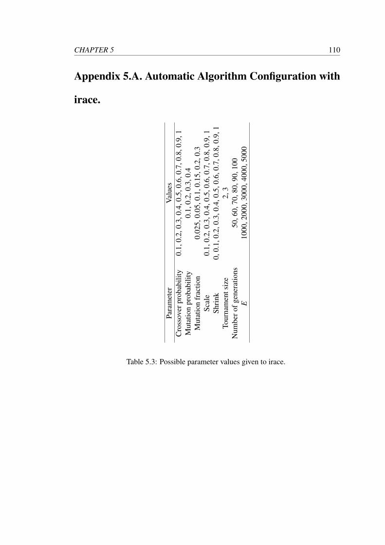
CHAPTER 5 110
Appendix 5.A. Automatic Algorithm Configuration with
irace.
Para
met
erV
alue
sC
ross
over
prob
abili
ty0.
1,0.
2,0.
3,0.
4,0.
5,0.
6,0.
7,0.
8,0.
9,1
Mut
atio
npr
obab
ility
0.1,
0.2,
0.3,
0.4
Mut
atio
nfr
actio
n0.
025,
0.05
,0.1
,0.1
5,0.
2,0.
3Sc
ale
0.1,
0.2,
0.3,
0.4,
0.5,
0.6,
0.7,
0.8,
0.9,
1Sh
rink
0,0.
1,0.
2,0.
3,0.
4,0.
5,0.
6,0.
7,0.
8,0.
9,1
Tour
nam
ents
ize
2,3
Num
bero
fgen
erat
ions
50,6
0,70
,80,
90,1
00E
1000
,200
0,30
00,4
000,
5000
Table 5.3: Possible parameter values given to irace.
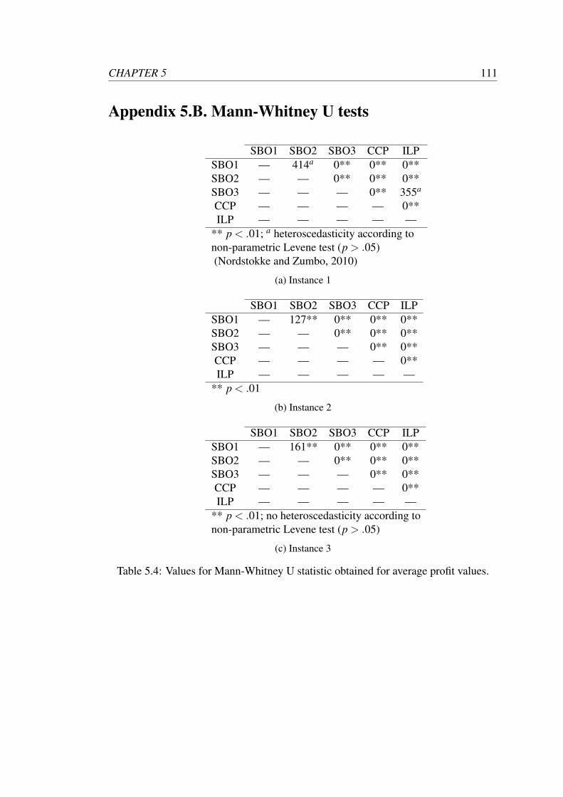
CHAPTER 5 111
Appendix 5.B. Mann-Whitney U tests
SBO1 SBO2 SBO3 CCP ILPSBO1 — 414a 0** 0** 0**SBO2 — — 0** 0** 0**SBO3 — — — 0** 355a
CCP — — — — 0**ILP — — — — —
** p < .01; a heteroscedasticity according tonon-parametric Levene test (p > .05)(Nordstokke and Zumbo, 2010)
(a) Instance 1
SBO1 SBO2 SBO3 CCP ILPSBO1 — 127** 0** 0** 0**SBO2 — — 0** 0** 0**SBO3 — — — 0** 0**CCP — — — — 0**ILP — — — — —
** p < .01
(b) Instance 2
SBO1 SBO2 SBO3 CCP ILPSBO1 — 161** 0** 0** 0**SBO2 — — 0** 0** 0**SBO3 — — — 0** 0**CCP — — — — 0**ILP — — — — —
** p < .01; no heteroscedasticity according tonon-parametric Levene test (p > .05)
(c) Instance 3
Table 5.4: Values for Mann-Whitney U statistic obtained for average profit values.
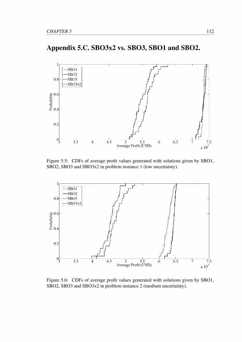
CHAPTER 5 112
Appendix 5.C. SBO3x2 vs. SBO3, SBO1 and SBO2.
Figure 5.5: CDFs of average profit values generated with solutions given by SBO1,SBO2, SBO3 and SBO3x2 in problem instance 1 (low uncertainty).
Figure 5.6: CDFs of average profit values generated with solutions given by SBO1,SBO2, SBO3 and SBO3x2 in problem instance 2 (medium uncertainty).
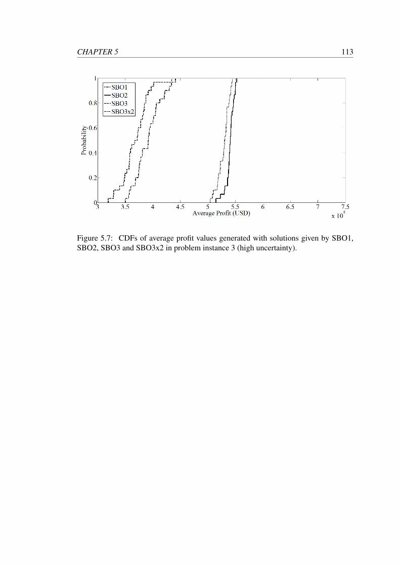
CHAPTER 5 113
Figure 5.7: CDFs of average profit values generated with solutions given by SBO1,SBO2, SBO3 and SBO3x2 in problem instance 3 (high uncertainty).
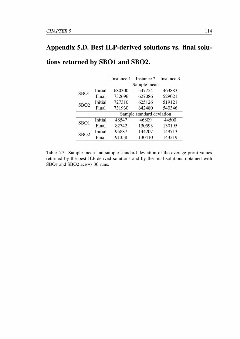
CHAPTER 5 114
Appendix 5.D. Best ILP-derived solutions vs. final solu-
tions returned by SBO1 and SBO2.
Instance 1 Instance 2 Instance 3Sample mean
SBO1Initial 680300 547754 463883Final 732696 627086 529021
SBO2Initial 727310 625126 519121Final 731930 642480 540346
Sample standard deviation
SBO1Initial 48547 46809 44500Final 82742 130593 130195
SBO2Initial 95887 144207 149713Final 91358 130410 143319
Table 5.5: Sample mean and sample standard deviation of the average profit valuesreturned by the best ILP-derived solutions and by the final solutions obtained withSBO1 and SBO2 across 30 runs.
Chapter 6
A Matheuristic Optimizer to Address
the d-MBKARS Problem
6.1 Abstract
In this chapter, we explore the potential of combining the global search mechanism of
a GA with the ability of ILP to generate a feasible (and optimal) production plan for
any given set of constraints. In particular, we use a GA to explore the space of capac-
ity values of failure-prone production lines, rather than searching through the space of
all possible production plans as done in Chapter 5. Here, the application of ILP can
be seen as a translation step that maps a solution given by the GA (genotype) onto
a production plan (phenotype). ILP is thus repeatedly called during the optimization
procedure and not only at the beginning, as occurs with both specialized initialization
operators from Chapter 5. We analyse the performance of this “matheuristic” opti-
mizer in the context of the real-world production planning problem addressed in the
previous chapter. Our results suggest that the approach performs well for problems
with low and medium uncertainty levels as it excludes unfeasible solutions from the
search space. However, we also find that the effectiveness of this approach decreases
115
CHAPTER 6 116
with increasing level of uncertainty. This can be explained by the restriction of the
accessible (phenotypic) search space to those production plans that are determined via
ILP: with increasing uncertainty, the real (non-linear) objective function becomes less
aligned with the (linear) objective function optimized in the ILP problem, limiting the
quality of solutions that can be reached through this search process.
6.2 Introduction
Most of the available techniques to address combinatorial optimization problems (Pin-
tea, 2014, p. 21) can be classified into two main categories: exact and heuristic ap-
proaches (Sorensen, 2015; Raidl and Puchinger, 2008). Exact approaches are able to
find a guaranteed optimal solution, but their computational time increases dramatically
with the scale of the problem, and thus its applicability to address real-world problems
is usually limited. Therefore, in many real-world applications optimality is traded for
acceptable computational times by employing heuristic approaches.
General purpose heuristics are also known as meta-heuristics (Burke et al., 2009).
The term Meta-heuristics, first introduced by Glover (1986), is the composition of
two Greek words: the prefix “meta” and “heuriskein”, which mean “beyond” and “to
find”, respectively. Meta-heuristics are high level search strategies (as revealed by its
meaning), able to return solutions, not necessarily optimal (Caserta and Voß, 2009), in
acceptable computational times by implementing a search that tries to balance diversi-
fication (exploration) and intensification (exploitation) (Blum and Roli, 2008).
The combination of exact and meta-heuristic approaches seems ideal by drawing
upon the strengths of both streams. However, it is only in recent years that the poten-
tial of hybrid meta-heuristics is being recognized in the optimization community (Raidl
and Puchinger, 2008). In the broad sense, the term hybrid meta-heuristic refers to the
CHAPTER 6 117
combination of a meta-heuristic with any other optimization technique, e.g. mathe-
matical programming methods, heuristic methods or other meta-heuristics (Blum and
Roli, 2008). More specifically, approaches that combine meta-heuristics with math-
ematical programming techniques are known as matheuristics (Villegas et al., 2013).
This relatively new area of research has captured the attention of a growing research
community (Boschetti et al., 2009), which is reflected in an increasing number of pub-
lications (Caserta and Voß, 2013; Blum et al., 2011; Blum and Roli, 2008; Raidl and
Puchinger, 2008; Puchinger and Raidl, 2005; Raidl, 2006; Talbi, 2002).
Therefore, in line with this research trend we investigate in this chapter a new SBO
approach that employs a matheuristic optimizer to address the d-MBKARS problem.
The success of the matheuristic approaches (SBO1 and SBO2) introduced in Chap-
ter 5, provided supporting evidence of the synergies resulting from the combination
of mathematical programming techniques with a population-based meta-heuristic op-
timizer, namely a GA. In those approaches, ILP was only called at the beginning of
the optimization to initialize part of the GA initial population. In this chapter, we
investigate whether synergies between both techniques can be further exploited, by
developing a matheuristic optimizer where mathematical programming techniques are
repeatedly called during the optimization (not only at the beginning).
The motivation behind the approach presented here, latter referred to as SBOMat,
is to create a search space for the meta-heuristic, in this case a GA, where all possible
solutions are feasible and then apply ILP as a translation tool able to map every solution
given by the GA onto a feasible production plan. The use of mathematical program-
ming techniques may facilitate the generation of feasible solutions under constrained
settings, a difficult task for meta-heuristics such as GAs, where standard genetic op-
erators like crossover and mutation could potentially turn high quality solutions into
unfeasible ones.
CHAPTER 6 118
6.3 SBOMat Approach
As presented in Chapter 5, the original formulation of the d-MBKARS problem is as
follows:
maximize f (x) =n
∑j=1
∑l∈A j
v j× sl, j− k j× (xl, j− sl, j) (6.1)
subject to
n
∑j=1
∑l∈A j
wi, j× xl, j ≤ ci (i = 1,2, . . . ,d), (6.2)
∑l∈A j
xl, j 6 b j (xl, j ∈ Z≥0; j = 1,2, . . . ,n). (6.3)
In order to introduce the SBOMat approach, it is necessary to add to the original
formulation a new set of constraints in the form of Equation 6.4 to separately capture
the capacity requirements of failure-prone production lines, leaving the rest of resource
constraints represented in the form of Equation 6.2.
n
∑j=1
wl, j× xl, j ≤ c′l (l = 1,2, . . . ,m). (6.4)
The main difference between SBOMat and the SBO approaches presented in Chap-
ter 5 is that the former uses a GA to search for capacity values of failure-prone produc-
tion lines, namely the RHS c′l of Equation 6.4, whereas the latter uses a GA to directly
search for a production plan x. As illustrated in Figure 6.1, the SBOMat approach first
generates a population of solutions, where each solution is denoted here as c’ (vector
of c′l), and then employs ILP as a translation tool able to generate a production plan
x (phenotype), given the set of constraints c’ (genotype) determined by the GA. This
second step is performed by optimizing, via ILP, Equation 6.5 subject to the sets of
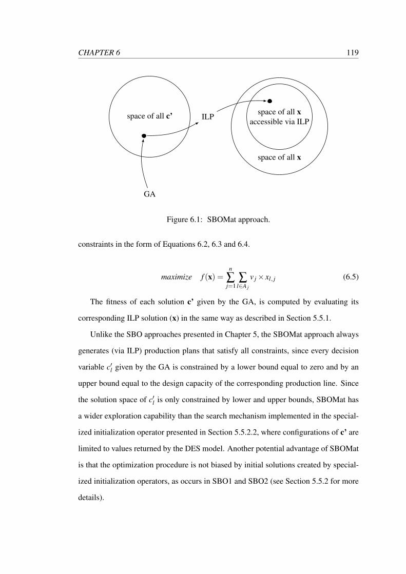
CHAPTER 6 119
space of all c’space of all x
space of all x
space of all xaccessible via ILP
GA
ILP
Figure 6.1: SBOMat approach.
constraints in the form of Equations 6.2, 6.3 and 6.4.
maximize f (x) =n
∑j=1
∑l∈A j
v j× xl, j (6.5)
The fitness of each solution c’ given by the GA, is computed by evaluating its
corresponding ILP solution (x) in the same way as described in Section 5.5.1.
Unlike the SBO approaches presented in Chapter 5, the SBOMat approach always
generates (via ILP) production plans that satisfy all constraints, since every decision
variable c′l given by the GA is constrained by a lower bound equal to zero and by an
upper bound equal to the design capacity of the corresponding production line. Since
the solution space of c′l is only constrained by lower and upper bounds, SBOMat has
a wider exploration capability than the search mechanism implemented in the special-
ized initialization operator presented in Section 5.5.2.2, where configurations of c’ are
limited to values returned by the DES model. Another potential advantage of SBOMat
is that the optimization procedure is not biased by initial solutions created by special-
ized initialization operators, as occurs in SBO1 and SBO2 (see Section 5.5.2 for more
details).
CHAPTER 6 120
6.4 Benchmark Analysis
In order to analyse the performance of SBOMat, we apply it to the real-world problem
analysed in Chapter 5 and compare its results against the ones returned by the SBO1
and SBO2 models, proposed in Chapter 5.
To enable a fair comparison, all different strategies employ the same GA (see Chap-
ter 5 for details about the GA), the optimization is performed across 50 generations
based on a population size of 40 individuals and the computational budget (E) al-
located to the final solution selection is 3000 fitness evaluations. However, neither
the specialized initialization operators (see Section 5.5.2) nor the repair operator (see
Section 5.5.3) are applied to SBOMat. The parameter configuration of this GA was
determined separately for SBOMat based on preliminary experimentation and is as
follows: uniform crossover (crossover probability: 0.8), Gaussian mutation (mutation
probability: 0.2, mutation fraction: 0.33, scale: 0.5 and shrink: 0.1) and tournament
selection (tournament size: 2).
In line with our previous experiments with SBO1 and SBO2, we execute 30 runs of
SBOMat for the three problem instances analysed in Chapter 5. Here, we also use dif-
ferent seeds for the random number generator in every run. We compute average profit
values for every final solution returned by SBOMat, across a sample of 5000 profit
values obtained via stochastic simulation, and then use those estimates to evaluate the
optimization performance of SBOMat against SBO1 and SBO2.
6.5 Results
Our results reveal that under low and medium uncertainty levels (problem instance 1
and 2), the SBOMat approach outperformed (p < .01) SBO1 and SBO2 in terms of op-
timization performance, but evidenced a performance comparable (p > .05) to SBO2
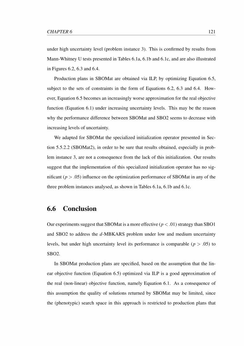
CHAPTER 6 121
under high uncertainty level (problem instance 3). This is confirmed by results from
Mann-Whitney U tests presented in Tables 6.1a, 6.1b and 6.1c, and are also illustrated
in Figures 6.2, 6.3 and 6.4.
Production plans in SBOMat are obtained via ILP, by optimizing Equation 6.5,
subject to the sets of constraints in the form of Equations 6.2, 6.3 and 6.4. How-
ever, Equation 6.5 becomes an increasingly worse approximation for the real objective
function (Equation 6.1) under increasing uncertainty levels. This may be the reason
why the performance difference between SBOMat and SBO2 seems to decrease with
increasing levels of uncertainty.
We adapted for SBOMat the specialized initialization operator presented in Sec-
tion 5.5.2.2 (SBOMat2), in order to be sure that results obtained, especially in prob-
lem instance 3, are not a consequence from the lack of this initialization. Our results
suggest that the implementation of this specialized initialization operator has no sig-
nificant (p > .05) influence on the optimization performance of SBOMat in any of the
three problem instances analysed, as shown in Tables 6.1a, 6.1b and 6.1c.
6.6 Conclusion
Our experiments suggest that SBOMat is a more effective (p< .01) strategy than SBO1
and SBO2 to address the d-MBKARS problem under low and medium uncertainty
levels, but under high uncertainty level its performance is comparable (p > .05) to
SBO2.
In SBOMat production plans are specified, based on the assumption that the lin-
ear objective function (Equation 6.5) optimized via ILP is a good approximation of
the real (non-linear) objective function, namely Equation 6.1. As a consequence of
this assumption the quality of solutions returned by SBOMat may be limited, since
the (phenotypic) search space in this approach is restricted to production plans that
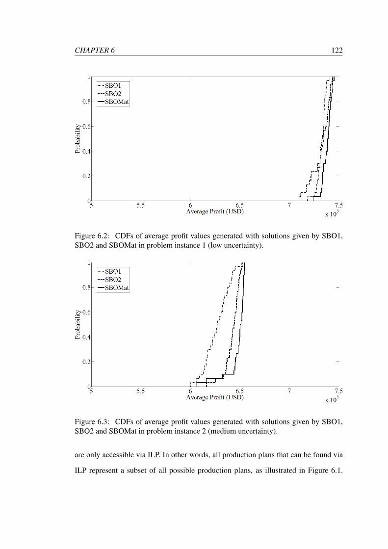
CHAPTER 6 122
Figure 6.2: CDFs of average profit values generated with solutions given by SBO1,SBO2 and SBOMat in problem instance 1 (low uncertainty).
Figure 6.3: CDFs of average profit values generated with solutions given by SBO1,SBO2 and SBOMat in problem instance 2 (medium uncertainty).
are only accessible via ILP. In other words, all production plans that can be found via
ILP represent a subset of all possible production plans, as illustrated in Figure 6.1.
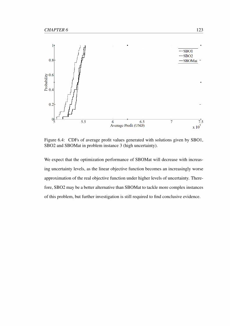
CHAPTER 6 123
Figure 6.4: CDFs of average profit values generated with solutions given by SBO1,SBO2 and SBOMat in problem instance 3 (high uncertainty).
We expect that the optimization performance of SBOMat will decrease with increas-
ing uncertainty levels, as the linear objective function becomes an increasingly worse
approximation of the real objective function under higher levels of uncertainty. There-
fore, SBO2 may be a better alternative than SBOMat to tackle more complex instances
of this problem, but further investigation is still required to find conclusive evidence.
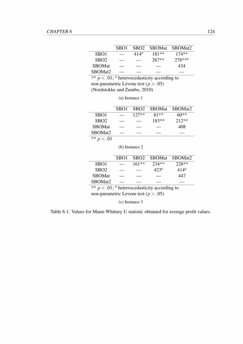
CHAPTER 6 124
SBO1 SBO2 SBOMat SBOMat2SBO1 — 414a 181** 174**SBO2 — — 267** 278**a
SBOMat — — — 434SBOMat2 — — — —** p < .01; a heteroscedasticity according tonon-parametric Levene test (p > .05)(Nordstokke and Zumbo, 2010)
(a) Instance 1
SBO1 SBO2 SBOMat SBOMat2SBO1 — 127** 81** 60**SBO2 — — 183** 212**
SBOMat — — — 408SBOMat2 — — — —** p < .01
(b) Instance 2
SBO1 SBO2 SBOMat SBOMat2SBO1 — 161** 234** 228**SBO2 — — 423a 414a
SBOMat — — — 447SBOMat2 — — — —** p < .01; a heteroscedasticity according tonon-parametric Levene test (p > .05)
(c) Instance 3
Table 6.1: Values for Mann-Whitney U statistic obtained for average profit values.
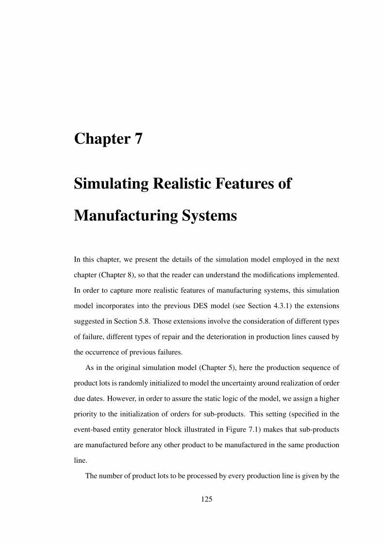
Chapter 7
Simulating Realistic Features of
Manufacturing Systems
In this chapter, we present the details of the simulation model employed in the next
chapter (Chapter 8), so that the reader can understand the modifications implemented.
In order to capture more realistic features of manufacturing systems, this simulation
model incorporates into the previous DES model (see Section 4.3.1) the extensions
suggested in Section 5.8. Those extensions involve the consideration of different types
of failure, different types of repair and the deterioration in production lines caused by
the occurrence of previous failures.
As in the original simulation model (Chapter 5), here the production sequence of
product lots is randomly initialized to model the uncertainty around realization of order
due dates. However, in order to assure the static logic of the model, we assign a higher
priority to the initialization of orders for sub-products. This setting (specified in the
event-based entity generator block illustrated in Figure 7.1) makes that sub-products
are manufactured before any other product to be manufactured in the same production
line.
The number of product lots to be processed by every production line is given by the
125
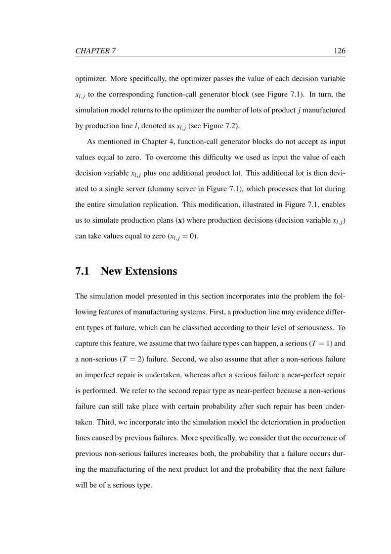
CHAPTER 7 126
optimizer. More specifically, the optimizer passes the value of each decision variable
xl, j to the corresponding function-call generator block (see Figure 7.1). In turn, the
simulation model returns to the optimizer the number of lots of product j manufactured
by production line l, denoted as sl, j (see Figure 7.2).
As mentioned in Chapter 4, function-call generator blocks do not accept as input
values equal to zero. To overcome this difficulty we used as input the value of each
decision variable xl, j plus one additional product lot. This additional lot is then devi-
ated to a single server (dummy server in Figure 7.1), which processes that lot during
the entire simulation replication. This modification, illustrated in Figure 7.1, enables
us to simulate production plans (x) where production decisions (decision variable xl, j)
can take values equal to zero (xl, j = 0).
7.1 New Extensions
The simulation model presented in this section incorporates into the problem the fol-
lowing features of manufacturing systems. First, a production line may evidence differ-
ent types of failure, which can be classified according to their level of seriousness. To
capture this feature, we assume that two failure types can happen, a serious (T = 1) and
a non-serious (T = 2) failure. Second, we also assume that after a non-serious failure
an imperfect repair is undertaken, whereas after a serious failure a near-perfect repair
is performed. We refer to the second repair type as near-perfect because a non-serious
failure can still take place with certain probability after such repair has been under-
taken. Third, we incorporate into the simulation model the deterioration in production
lines caused by previous failures. More specifically, we consider that the occurrence of
previous non-serious failures increases both, the probability that a failure occurs dur-
ing the manufacturing of the next product lot and the probability that the next failure
will be of a serious type.
CHAPTER 7 127
Figure 7.1: Order initialization sub-system of production line 2.
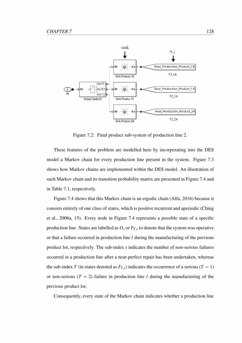
CHAPTER 7 128
Figure 7.2: Final product sub-system of production line 2.
These features of the problem are modelled here by incorporating into the DES
model a Markov chain for every production line present in the system. Figure 7.3
shows how Markov chains are implemented within the DES model. An illustration of
such Markov chain and its transition probability matrix are presented in Figure 7.4 and
in Table 7.1, respectively.
Figure 7.4 shows that this Markov chain is an ergodic chain (Alfa, 2016) because it
consists entirely of one class of states, which is positive recurrent and aperiodic (Ching
et al., 2006a, 15). Every node in Figure 7.4 represents a possible state of a specific
production line. States are labelled as Os or FT,s to denote that the system was operative
or that a failure occurred in production line l during the manufacturing of the previous
product lot, respectively. The sub-index s indicates the number of non-serious failures
occurred in a production line after a near-perfect repair has been undertaken, whereas
the sub-index T (in states denoted as FT,s) indicates the occurrence of a serious (T = 1)
or non-serious (T = 2) failure in production line l during the manufacturing of the
previous product lot.
Consequently, every state of the Markov chain indicates whether a production line
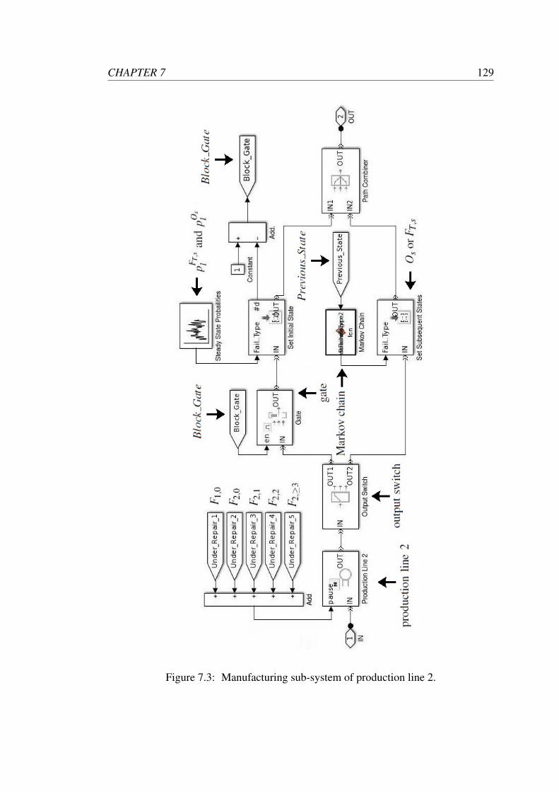
CHAPTER 7 129
Figure 7.3: Manufacturing sub-system of production line 2.
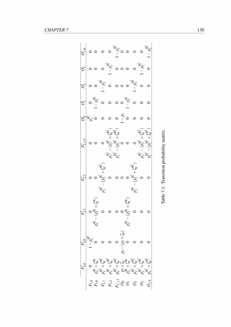
CHAPTER 7 130
F′ 1,
0F′ 2,
0F′ 2,
1F′ 2,
2F′ 2,≥
3O′ 0
O′ 1
O′ 2
O′ 3
O′ ≥
4
F 1,0
01−
pϕ4 l
l0
00
pϕ4 l
l0
00
0F 2
,0pϕ
ll×
ζϕ
ll
0pϕ
ll−(p
ϕl
l×
ζϕ
ll)
00
01−
pϕl
l0
00
F 2,1
pϕ2 l
l×
ζϕ
2 ll
00
pϕ2 l
l−(p
ϕ2 l
l×
ζϕ
2 ll)
00
01−
pϕ2 l
l0
0
F 2,2
pϕ3 l
l×
ζϕ
3 ll
00
0pϕ
3 ll−(p
ϕ3 l
l×
ζϕ
3 ll)
00
01−
pϕ3 l
l0
F 2,≥
3pϕ
4 ll×
ζϕ
4 ll
00
0pϕ
4 ll−(p
ϕ4 l
l×
ζϕ
4 ll)
00
00
1−
pϕ4 l
lO
0p l×
ζl
p l−(p
l×ζ
l)0
00
1−
p l0
00
0O
1pϕ
ll×
ζϕ
ll
0pϕ
ll−(p
ϕl
l×
ζϕ
ll)
00
01−
pϕl
l0
00
O2
pϕ2 l
l×
ζϕ
2 ll
00
pϕ2 l
l−(p
ϕ2 l
l×
ζϕ
2 ll)
00
01−
pϕ2 l
l0
0
O3
pϕ3 l
l×
ζϕ
3 ll
00
0pϕ
3 ll−(p
ϕ3 l
l×
ζϕ
3 ll)
00
01−
pϕ3 l
l0
O≥
4pϕ
4 ll×
ζϕ
4 ll
00
0pϕ
4 ll−(p
ϕ4 l
l×
ζϕ
4 ll)
00
00
1−
pϕ4 l
l
Tabl
e7.
1:Tr
ansi
tion
prob
abili
tym
atri
x.
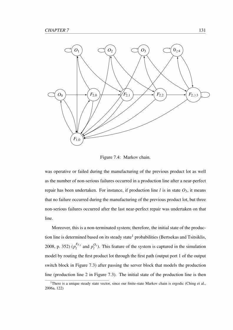
CHAPTER 7 131
F1,0
O0
O1
F2,0
O2
F2,1
O3
F2,2
0≥4
F2,≥3
Figure 7.4: Markov chain.
was operative or failed during the manufacturing of the previous product lot as well
as the number of non-serious failures occurred in a production line after a near-perfect
repair has been undertaken. For instance, if production line l is in state O3, it means
that no failure occurred during the manufacturing of the previous product lot, but three
non-serious failures occurred after the last near-perfect repair was undertaken on that
line.
Moreover, this is a non-terminated system; therefore, the initial state of the produc-
tion line is determined based on its steady state1 probabilities (Bertsekas and Tsitsiklis,
2008, p. 352) (pFT,sl and pOs
l ). This feature of the system is captured in the simulation
model by routing the first product lot through the first path (output port 1 of the output
switch block in Figure 7.3) after passing the server block that models the production
line (production line 2 in Figure 7.3). The initial state of the production line is then
1There is a unique steady state vector, since our finite-state Markov chain is ergodic (Ching et al.,2006a, 122)
CHAPTER 7 132
set as an attribute on that first product lot, based on the realization of a discrete ran-
dom variable. Every outcome of this random variable represents a state in the Markov
chain and it is realized according to the corresponding steady state probabilities. Once
the first product lot has passed through, this first path is no longer accessible to any
subsequent lot until the end of the simulation replication. This first path is blocked by
a gate (see gate block in Figure 7.3) which forbids entity arrivals (product lots) when
Block Gate 6 0 (where the signal Block Gate = 1− number of entities departed from
the attribute block which sets the initial state of the production line).
Except for the initial state, every subsequent state of a production line is determined
by the corresponding Markov chain, based exclusively on the transition probabilities
of its previous state. Here, a Markov chain is triggered every time a product lot needs
to be manufactured by the corresponding production line. The information about the
state of the production line is then passed to the DES model, where it is set as an
attribute on each product lot. Those attributes determine the route to be followed by a
product lot. More specifically, the state (FT,s or Os) of a production line is an attribute
that specifies the output port through which a product lot is routed when it arrives to
the output switch block shown in Figure 7.5.
Information about the previous state of the production line is given by the signal
Previous State (see Figure 7.3 and 7.5), which indicates the input port through which
the previous product lot arrived at the path combiner block illustrated in Figure 7.5.
This signal is then used as input for the Markov chain (see Figure 7.3) when the next
product lot arrives. For simplicity, we assume that the transition probabilities of every
state can be calculated as shown in Table 7.1. pl is the probability that a production
line failure occurs (either serious or non-serious) during the manufacturing of the next
product lot, given that the production line is in state O0 (i.e. no non-serious failure
has occurred after a near-perfect repair and the production line was operative during
the manufacturing of the previous product lot). ζl determines the probability that a
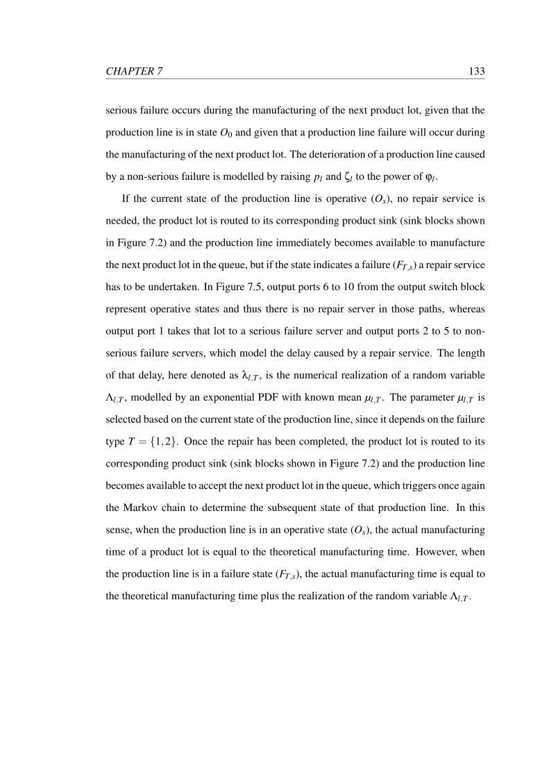
CHAPTER 7 133
serious failure occurs during the manufacturing of the next product lot, given that the
production line is in state O0 and given that a production line failure will occur during
the manufacturing of the next product lot. The deterioration of a production line caused
by a non-serious failure is modelled by raising pl and ζl to the power of ϕl .
If the current state of the production line is operative (Os), no repair service is
needed, the product lot is routed to its corresponding product sink (sink blocks shown
in Figure 7.2) and the production line immediately becomes available to manufacture
the next product lot in the queue, but if the state indicates a failure (FT,s) a repair service
has to be undertaken. In Figure 7.5, output ports 6 to 10 from the output switch block
represent operative states and thus there is no repair server in those paths, whereas
output port 1 takes that lot to a serious failure server and output ports 2 to 5 to non-
serious failure servers, which model the delay caused by a repair service. The length
of that delay, here denoted as λl,T , is the numerical realization of a random variable
Λl,T , modelled by an exponential PDF with known mean µl,T . The parameter µl,T is
selected based on the current state of the production line, since it depends on the failure
type T = 1,2. Once the repair has been completed, the product lot is routed to its
corresponding product sink (sink blocks shown in Figure 7.2) and the production line
becomes available to accept the next product lot in the queue, which triggers once again
the Markov chain to determine the subsequent state of that production line. In this
sense, when the production line is in an operative state (Os), the actual manufacturing
time of a product lot is equal to the theoretical manufacturing time. However, when
the production line is in a failure state (FT,s), the actual manufacturing time is equal to
the theoretical manufacturing time plus the realization of the random variable Λl,T .
CHAPTER 7 134
Figure 7.5: Repair sub-system of production line 2.
CHAPTER 7 135
7.2 Conclusion
The combination of DES and Markov chains provides a great flexibility to model real-
istic features of manufacturing systems. Markov chains enable us to keep track of the
current state of a production line, and based on that information we can dynamically
modify the different probabilities governing the system in order to model the occur-
rence and non-occurrence of failures in a more realistic manner. At the same time, this
simulation approach enables us to consider different types of repair, e.g. near-perfect
and imperfect repairs, and different failure types, i.e. the expected delay caused by
repair services (µl,T ) depends on the failure type T = 1,2, where µl,1 > µl,2. Finally,
given that the probabilities of having serious and non-serious failures depend on the
state of the production line (which accounts for near-perfect and imperfect repairs un-
dertaken as well as the number of non-serious failures occurred previously), we can
incorporate into the simulation model the deterioration caused by previous failures.
Chapter 8
Evolutionary Robust Optimization
(Manuscript 4)
J. E. Diaz, J. Handl, and D.-L. Xu. Single and Multi-objective Formulations for Evo-
lutionary Robust Optimization - Interaction between Sample Size and Choice of Ro-
bustness Measure. Computers & Operations Research, Submitted, 2015.
8.1 Abstract
In this chapter, we aim to find robust solutions in optimization settings where there
is uncertainty associated with the operating/environmental conditions, and the fitness
of a solution is hence best described by a distribution of outcomes. In such settings,
the nature of the fitness distribution (reflecting the performance of a particular solution
across a set of operating scenarios) is of potential interest in deciding solution quality,
and this is something that has not been analysed yet in previous chapters. Previous
work has suggested the inclusion of robustness as an additional optimization objec-
tive. However, there has been limited investigation of different robustness criteria, and
the impact this choice may have on the sample size needed to obtain reliable fitness
136

CHAPTER 8 137
estimates. Here, we investigate different single and multi-objective formulations for
robust optimization, in the context of a real-world problem addressed via SBO. For
the (limited computational budget) setting considered here, our results highlight the
value of an explicit robustness criterion in steering an optimizer towards solutions that
are not only robust (as may be expected), but also associated with a profit that is, on
average, higher than that identified by standard single-objective approaches. We also
observe significant interactions between the choice of robustness measure and the sam-
ple size employed during fitness evaluation, an effect that is more pronounced for our
multi-objective models.
8.2 Introduction
Real-world problems often require the consideration of multiple and often conflict-
ing criteria (Deb, 2014; Wang et al., 2015; Mlakar et al., 2015). When faced with
problems that incorporate uncertainty, one may arguably need to take into account the
robustness of solutions (Branke and Lu, 2015) as an additional criterion of solution
quality. Ideally, robust optimization would identify a solution that simultaneously of-
fers the best and most robust performance; in reality, these two criteria are usually
conflicting (Rooderkerk and Van Heerde, 2016), and a single optimal solution is un-
likely to exist. Due to this expected trade-off between the quality of a solution and its
robustness (Jin and Branke, 2005; Paenke et al., 2006), methodologies that are capable
of identifying a desirable trade-off between these conflicting criteria are of significant
interest in a robust optimization setting.
A complicating factor in robust optimization is the lack of a unique definition of
the robustness of a solution. In some cases a solution is considered to be robust when,
under certain levels of variation in the decision space1, it performs reasonably well in
1Here we deal with variation in the decision space, which in turn generates variation in the objective
CHAPTER 8 138
terms of quality (e.g. expected objective value) (Goh and Tan, 2009, p. 189), feasibility
or optimality (Gabrel et al., 2014). Perhaps a more common idea is to consider as
robust a solution that offers the best performance under the worst-case scenario (Gabrel
et al., 2014) (e.g. maximizing the minimum value of a performance measure).
Independent of the exact definition of robustness, it has been argued that it may be
advantageous to explicitly consider robustness as a separate objective (Jin and Send-
hoff, 2003), instead of optimizing for a single measure that implicitly considers robust-
ness (e.g. the average of a performance measure). This is because, in doing so (using
e.g. a Pareto optimization approach), the trade-off between the main objective and its
robustness measure may become more evident and facilitate decision making. On the
other hand, more implicit considerations of robustness may have advantages in terms
of the associated computational expense and their ease of implementation.
When EAs are applied as optimizers in single and multi-objective optimization
problems, both approaches have a natural tendency to return robust solutions due to
the implicit averaging mechanism intrinsic to an EA (Branke, 1998; Jin and Branke,
2005; Tsutsui and Ghosh, 1997). This tendency is emphasized further when explicit
averaging (Jin and Branke, 2005) is implemented as a noise handling strategy. Given
the above, our study sets out to investigate the extent to which evolutionary single-
objective (ESO) optimization approaches (using an explicit averaging scheme) are al-
ready able to generate trade-off solutions between performance and robustness, and to
what extent (and under what circumstances) these solutions are improved by evolu-
tionary multi-objective (EMO) optimization approaches that consider robustness as a
concrete optimization objective.
space.
CHAPTER 8 139
8.2.1 Robust Optimization
To some extent, robust solutions to a problem may be obtained by replacing the original
objective(s) by its/their “robust” equivalent(s) (Jin and Branke, 2005), e.g. a robustness
measure such as the average value instead of a single evaluation. Alternatively, mea-
sures of robustness may be integrated into the optimization as hard constraints (Goh
and Tan, 2009, p. 216). A third possibility is to consider robustness as part of a compos-
ite function that is the weighted sum of different objectives (Deb, 2014, p. 408; Guo
et al., 2008). This is, of course, a standard approach to transform a multi-objective
optimization problem into a single-objective optimization problem, with a number of
known limitations: the choice of appropriate values for the weight vector can be dif-
ficult and highly subjective, as it requires the translation of qualitative information
into quantitative indicators (Deb, 2014, p. 409). Furthermore, the (single) solution ob-
tained through this approach can be very sensitive to the relative weight assigned to
each objective, and the method may thus be highly-user dependent. Although different
solutions can be found by varying the weights, this approach is unable to find Pareto
optimal solutions that lie on non-convex regions of the Pareto optimal front (Marler
and Arora, 2010).
Pareto optimization overcomes these limitations by exploring different trade-off
solutions between a set of objectives (Handl et al., 2007). This approach requires no
prior knowledge of a preference vector and it returns a set of Pareto-optimal solutions
to the decision maker. Thus, in Pareto optimization the aim is not only to find an op-
timal or near-optimal solution, but a set of diverse solutions of equal quality, called
Pareto-optimal set. Solutions from this set dominate all solutions outside this set and
none of them dominates other solution within this set. A solution dominates other so-
lution if it is strictly better in at least one objective and not worse in any objective (Deb
and Gupta, 2006; Lopez-Ibanez et al., 2010). The reader is referred to Deb (2014)
CHAPTER 8 140
and Coello (2006) for more details about common concepts in Pareto optimization. In
the context of robust optimization, we may use Pareto optimization to simultaneously
optimize the original objective (performance measure) as well as a robustness measure.
The Pareto front then serves to illustrate the trade-off between these objectives, and the
decision maker may choose one solution from the set of Pareto-optimal solutions based
on his experience and specific requirements.
8.2.2 Evolutionary Robust Optimization
Several previous works have searched for robust solutions via ESO optimization. Tsut-
sui and Ghosh (1997) proposed the single-evaluation mode (SEM) for GAs with a ro-
bust solution searching scheme, which consists of adding perturbations to the values of
the decision variables, and then a single fitness evaluation is computed per individual.
Under the SEM approach robust individuals are more likely to survive across genera-
tions than less robust ones. SEM can be seen as an equivalent to an implicit averaging
strategy when uncertainty is present in the decision space. Also a multi-evaluation
mode (MEM), which is equivalent to an explicit averaging strategy, was later proposed
by Tsutsui (1999) to search for robust solutions with GAs. The author also proposed a
MEM where the fitness of an individual corresponds to the worst fitness value (MEM-
W) for situations where robustness is a crucial consideration. Branke (1998) analysed
the potential of EAs to find robust solutions via different explicit averaging strategies.
In Branke (1998), uncertainty is also modelled by adding random perturbations to the
decision space before fitness evaluation. After analysing several strategies, the author
concluded that both, re-evaluating fitter individuals and using previous fitness values
to weight the fitness of those individuals are two promising ways to help EAs in the
search for robust solutions. The MEM-W approach proposed by Tsutsui (1999) is later
applied by Ong et al. (2006) within a max-min surrogate-assisted EA to generate robust
CHAPTER 8 141
solutions for engineering design, since MEM-W was thought to be more conservative
in terms of solution robustness than MEM (explicit averaging).
Considerable research in robust optimization can also be found in the existing EMO
optimization literature. The explicit averaging strategy used in ESO optimization was
extended to EMO optimization by Deb and Gupta (2006). Two approaches to obtain
robust solutions are proposed in Deb and Gupta (2006). In the first approach, fitness
evaluations for the different objectives are computed by averaging a set of neighbour-
ing solutions in order to create perturbations in the decision space, which are later
reflected in the objective space. In the second approach the optimization is performed
based on fitness evaluations of the actual individuals (without perturbations) present in
the population and a constraint is added to the problem per every objective considered.
This constraint limits to a user-defined value the normalized, absolute or average nor-
malized difference between the perturbed fitness (which according to the authors can
be the average fitness or the worst fitness) and the original fitness (fitness of the actual
solution without perturbations). In this second approach the user can define the desired
level of robustness, since it is possible to limit the level of functional change caused
by local perturbations. In both approaches multiple fitness evaluations need to be com-
puted (using neighbouring solutions) to calculate the average fitness and the perturbed
fitness in the first and second case, respectively. In Jin and Sendhoff (2003), trade-off
solutions between robustness and performance were obtained by simultaneously op-
timizing both criteria via EMO optimization. According to Jin and Sendhoff (2003)
expectation measures such as the sample mean cannot sufficiently capture fluctuations
in performance, whereas variance-based measures fail to take into account the absolute
performance of a solution, thus both measures should be considered as two individual
objectives in the search for robust solutions. This idea of simultaneously optimizing
a performance and a robustness measure via EMO optimization has been applied in
several studies to search for robust solutions. For instance, Ray (2002) searched for
CHAPTER 8 142
robust solutions for engineering design problems by simultaneously optimizing via
EMO optimization a performance measure, in this case the average performance of
neighbouring solutions, and the standard deviation of the performance of neighbour-
ing solutions. Goh and Tan (2007) generated trade-off solutions between performance
and robustness via EMO optimization by optimizing a performance measure and the
worst case performance as the robustness measure.
While many single and multi-objective studies have been published in the field of
robust optimization, studies that directly compare ESO and EMO approaches to find
robust solutions for the same problem are rare in the existing literature. Pereira et al.
(2015) compared the ability of evolutionary single and multi-objective algorithms to
find robust solutions (link weight configurations for traffic routing processes). How-
ever, in Pereira et al. (2015) a solution was considered to be robust when it performed
well under two different network conditions; in this sense, two performance measures
(rather than one performance measure and one robustness measure) were optimized.
The weighted sum of two congestion functions (two performance measures) was ap-
plied as fitness function in the ESO algorithm, whereas in both EMO algorithms, the
non-dominated sorting genetic algorithm II (NSGA II) (Deb et al., 2002) and strength
Pareto evolutionary algorithm 2, both congestion functions were optimized separately.
The performance advantage of NSGA II was evident under more complex network
topologies and more demanding traffic requirements.
8.2.3 Contributions
In this chapter, we investigate the extent to which ESO and EMO optimization are
able to generate comparable trade-off solutions between performance and robustness
by analysing the sets of non-dominated solutions obtained with the single and multi-
objective algorithms introduced in Section 8.3.1.1. Those non-dominated solutions are
CHAPTER 8 143
identified based on estimates computed via stochastic simulation for the sample mean,
sample standard deviation and sample minimum of every feasible solution present in
the final population obtained with the different models analysed.
Furthermore, we investigate how the use of the sample minimum as robustness
measure may affect the optimization performance of EAs compared to the use of less
biased statistics such as the sample mean or the sample standard deviation. While,
many measures of robustness have been proposed in the existing literature (Goh et al.,
2010), the sample minimum (worst case scenario for maximization problems) is par-
ticularly popular (Gabrel et al., 2014), see Chen et al. (2016), Zhang et al. (2016), Goh
and Tan (2007), Ong et al. (2006) and Tsutsui (1999) for some examples. It is also often
stated that by using the sample minimum as robustness measure more robust solutions
can be obtained (Ong et al., 2006; Tsutsui, 1999). However, very limited attention has
been given to how the choice of a robustness measure may affect the optimization per-
formance of single and multi-objective EAs, and how the sample minimum compares
to other measures. As statistics tell us that the sample minimum is a biased estimator
for the population (Lopez-Ibanez et al., 2010), it is possible that the use of the sample
minimum as a robustness measure may mislead the selection operator and steer the EA
towards undesirable regions of the objective space.
Finally, we investigate how the level of noise in fitness estimates (which we di-
rectly control through the sample size used during fitness evaluation) affects the op-
timization performance of the single and multi-objective optimizers analysed. Since
we allocate the same computational budget (total number of simulation replications)
to all optimization runs across models, more reliable fitness estimates imply shorter
optimization runs (fewer generations). All three of these questions are considered for
different levels of uncertainty, in order to analyse how their answers may change with
increasing levels of uncertainty.
The remainder of this chapter is organized as follows: In Section 8.3, we introduce
CHAPTER 8 144
the problem analysed and describe the ESO and EMO models. In Section 8.4, we
introduce the details of the benchmark analysis, and the results obtained are presented
in Section 8.6. Finally, conclusions derived from this study are given in Section 8.7.
8.3 Simulation-Based Optimization Model
In production planning, profitability is not the only criterion that needs to be considered
during the specification of a production plan, but the robustness of that plan is also
relevant (Paenke et al., 2006).
In this study we address a production planning problem of a real manufacturing
system. Detailed features of this manufacturing system are presented in Chapter 2. The
robustness of production plans is a criterion that needs to be considered here because
the system analysed is subject to failures of its production lines, which may cause
deviations between a plan and its actual outcome. Consequently, we aim to identify
a set of production plans that makes evident the trade-off between profitability and
robustness, instead of being interested in finding the most profitable production plan in
terms of average profit as in Chapter 5.
Here, a production plan x is a vector of 41 decision variables, where each decision
variable xl, j indicates the number of lots of product j to be manufactured in production
line l during a finite planning horizon of one month. This batch manufacturing system
has a set M = 1,2, . . . ,7 of independent production lines and is able to manufacture
31 different products. A feature of this system is that only a subset A j ⊆ M of pro-
duction lines can manufacture a specific product j. Additionally, this manufacturing
system has insufficient capacity to fully cover demand requirements and is subject to
serious and non-serious failures of its production lines. We also consider that near-
perfect and imperfect repairs can be undertaken after the occurrence of a failure as
well as the deterioration caused by previous failures.
CHAPTER 8 145
SBO is an attractive approach to address this problem, for it can accurately capture
the inherent uncertainty and complexity of the manufacturing system, while searching
for near-optimal solutions for the problem analysed (Figueira and Almada-Lobo, 2014;
Syberfeldt et al., 2010; Ehrenberg and Zimmermann, 2012). The SBO model consists
of a simulation model and an EA coupled in a black-box fashion. Production plans
specified by the optimizer are simulated by the simulation model, which returns the
realization of that production plan. Those simulated responses are then used by the
optimizer to compute the fitness values of a given production plan.
The simulation model used in this study is the one presented in Chapter 7. This
simulation model developed in SimEventsr (The MathWorks, Inc., 2014) models the
manufacturing system analysed. It employs a combination of DES and Markov chains
to model realistic features of manufacturing systems such as different types of pro-
duction line failure, near-perfect and imperfect repairs as well as the deterioration of
production lines due to previous failures.
The reader is referred to Chapter 7 for a detailed description of the simulation
model, whereas further details about the optimization model are provided in Sec-
tion 8.3.1.
8.3.1 Optimization Model
In Chapter 5, we introduced the d-MBKARS problem as a generalization of the pro-
duction planning problem addressed in that chapter. Here, we address an extended
version of that problem that considers a robustness measure as a second objective.
In this problem we do not penalize deviations from a plan and we refer to it as the
multi-objective d-MBKARS (M-d-MBKARS) problem without penalty and its ILP
formulation, in the context of the problem analysed, is as follows:
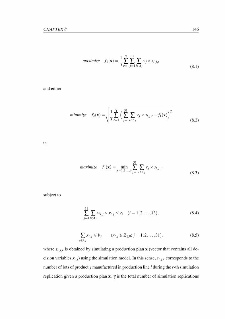
CHAPTER 8 146
maximize f1(x) =1γ
γ
∑r=1
31
∑j=1
∑l∈A j
v j× sl, j,r(8.1)
and either
minimize f2(x) =
√√√√1γ
γ
∑r=1
( 31
∑j=1
∑l∈A j
v j× sl, j,r− f1(x))2
(8.2)
or
maximize f3(x) = minr=1,2,...,γ
31
∑j=1
∑l∈A j
v j× sl, j,r(8.3)
subject to
31
∑j=1
∑l∈A j
wi, j× xl, j ≤ ci (i = 1,2, . . . ,13), (8.4)
∑l∈A j
xl, j 6 b j (xl, j ∈ Z≥0; j = 1,2, . . . ,31). (8.5)
where sl, j,r is obtained by simulating a production plan x (vector that contains all de-
cision variables xl, j) using the simulation model. In this sense, sl, j,r corresponds to the
number of lots of product j manufactured in production line l during the r-th simulation
replication given a production plan x. γ is the total number of simulation replications
CHAPTER 8 147
performed to compute fitness of a production plan, please see Section 8.3.1.1 for de-
tails about γ. The simulation model can be seen here as the function g(x) able to map
a production plan x onto the actual production sr (vector that contains all simulated
responses sl, j,r) without the requirement of a closed form formulation. In other words
sr is the realization of a production plan x during the r-th simulation replication. v j is
the marginal (per lot) contribution to profit of product j, wi, j is the amount of resource
i deployed by manufacturing one lot of product j and ci is the amount of resource i
available at the beginning of the manufacturing process.
We represent in the form of Equation 8.4 the design capacities of production lines,
the amount of labour needed to manufacture one lot of product j in production line l
and the situation where a product manufactured in this system is subsequently used as
raw material during the manufacturing of another product. We also impose additional
constraints in the form of Equation 8.5 to avoid that the production level of product j
exceeds its maximum demand b j. Please note that in this study, a production plan x is
feasible if it satisfies the set of constraints imposed as Equations 8.4 and 8.5.
8.3.1.1 Evolutionary Optimizers
For the multi-objective SBO (MSBO) approach, we require an optimizer able to find a
set of solutions that are non-dominated and are widely spread over the approximated
Pareto front. EAs are attractive optimizers for Pareto optimization not only due to their
wide applicability, flexibility (Coello, 2006) and ease of use (Coello, 2015), but also
because multiple non-dominated solutions can be found in a single iteration (Branke
et al., 2016; Deb, 2014; Coello, 2006). The optimizer used in the MSBO approach is
NSGA II, a well-known EMO algorithm commonly employed as benchmark in multi-
objective optimization (Coello, 2006), that has been successfully used to solve SBO
problems (see Brownlee and Wright (2015) and Sanchez et al. (2010) for recent exam-
ples).
CHAPTER 8 148
In the MSBO approach, in addition to optimizing a performance measure (max-
imize average profit), we simultaneously optimize a robustness measure in order to
explicitly capture as a second objective the robustness of a production plan. Two dif-
ferent measures of robustness are evaluated in the multi-objective approach, the stan-
dard deviation of profit and the minimum profit. The minimization of the standard
deviation tries to reduce the variation in profitability, whereas the maximization of the
minimum profit tries to improve the worst case scenario derived from a production
plan. In this sense the first MSBO model (MSBO-1) tries to simultaneously maximize
average profit (Equation 8.1) and minimize the standard deviation of profit (Equa-
tion 8.2), subject to the set of constraints in the form of Equations 8.4 and 8.5. The
second MSBO model (MSBO-2) differs from MSBO-1 in that, instead of minimiz-
ing the standard deviation, MSBO-2 tries to maximize minimum profit (Equation 8.3).
Both multi-objective models, MSBO-1 and MSBO-2, use NSGA II as optimizer.
Two different single-objective SBO (SSBO) models are also evaluated, the first
SSBO model (SSBO-1) tries to maximize average profit (Equation 8.1) subject to the
set of constraints in the form of Equations 8.4 and 8.5, whereas the second SSBO
model (SSBO-2) tries to maximize minimum profit (Equations 8.3), subject to the same
set of constraints. Both single-objective models employ as optimizer the MI-LXPM
algorithm proposed by Deep et al. (2009), but here, there is no need to implement a
final solution selection procedure (as done in Chapter 5, since we are interested in the
entire final population.
In order to make a fair comparison between MSBO and SSBO approaches, we
use the same parameters and operators for both optimizers, except for unavoidable
discrepancies that arise due to the different mechanics of both GAs. Both optimiz-
ers use a population size of 100 individuals and employ binary tournament selection,
Laplace crossover (crossover probability: 0.8) and power mutation (mutation proba-
bility: 0.005) as operators. See Deep et al. (2009) for more details about the last two
CHAPTER 8 149
operators and the parameter values used. Also the constraint-handling method pro-
posed by Deb (2000) and the truncation procedure described in Deep et al. (2009),
which ensures compliance with integer constraints after crossover and mutation, are
implemented in both optimizers.
It is important to mention that the selection criterion in NSGA II is based on the
crowded-comparison operator (Deb et al., 2002), although it employs a binary tourna-
ment selection operator. Moreover, the way elitism is incorporated in both optimizers
differs. In MI-LXPM, elitism is incorporated by having an elite set with a default size
of one (Deep and Thakur, 2007a,b). We do not adjust this parameter, as we are aiming
to maintain good levels of diversity throughout the optimization process. In NSGA II
elitism is incorporated by combining the entire parent and offspring populations before
extracting the new population.
Given the stochastic nature of simulation responses (sl, j,r) and due to the nature of
the objectives optimized (a sample of independent fitness values is required to com-
pute the fitness of an individual), all fitness values are computed across a number γ of
independent fitness evaluations. Two explicit averaging strategies are implemented in
every single and multi-objective model. In strategy A, fitness is computed across 10
independent fitness evaluations (γ = 10), whereas in strategy B, fitness is computed
across 30 independent fitness evaluations (γ = 30). The letter A or B is added to the
notation of the different models according to the explicit averaging strategy that they
employ, e.g. MSBO-1A and MSBO-1B.
Explicit averaging is a very expensive approach in terms of computational effort.
This computational expense becomes even more critical when explicit averaging is ap-
plied in the context of SBO, where expensive simulation replications are required to
compute multiple fitness values of entire populations. Therefore, in order to boost the
optimization performance of NSGA II and MI-LXPM, and reduce their computational
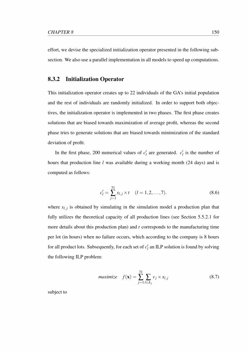
CHAPTER 8 150
effort, we devise the specialized initialization operator presented in the following sub-
section. We also use a parallel implementation in all models to speed up computations.
8.3.2 Initialization Operator
This initialization operator creates up to 22 individuals of the GA’s initial population
and the rest of individuals are randomly initialized. In order to support both objec-
tives, the initialization operator is implemented in two phases. The first phase creates
solutions that are biased towards maximization of average profit, whereas the second
phase tries to generate solutions that are biased towards minimization of the standard
deviation of profit.
In the first phase, 200 numerical values of c′l are generated. c′l is the number of
hours that production line l was available during a working month (24 days) and is
computed as follows:
c′l =31
∑j=1
sl, j× t (l = 1,2, . . . ,7). (8.6)
where sl, j is obtained by simulating in the simulation model a production plan that
fully utilizes the theoretical capacity of all production lines (see Section 5.5.2.1 for
more details about this production plan) and t corresponds to the manufacturing time
per lot (in hours) when no failure occurs, which according to the company is 8 hours
for all product lots. Subsequently, for each set of c′l an ILP solution is found by solving
the following ILP problem:
maximize f (x) =31
∑j=1
∑l∈A j
v j× xl, j (8.7)
subject to
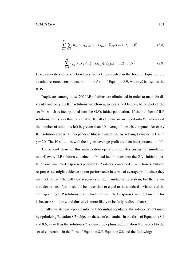
CHAPTER 8 151
31
∑j=1
∑l∈A j
wi, j× xl, j ≤ ci (xl, j ∈ Z≥0; i = 1,2, . . . ,6), (8.8)
31
∑j=1
wl, j× xl, j ≤ c′l (xl, j ∈ Z≥0; l = 1,2, . . . ,7). (8.9)
Here, capacities of production lines are not represented in the form of Equation 8.8
as other resource constraints, but in the form of Equation 8.9, where c′l is used as the
RHS.
Duplicates among those 200 ILP solutions are eliminated in order to maintain di-
versity and only 10 ILP solutions are chosen, as described bellow, to be part of the
set W , which is incorporated into the GA’s initial population. If the number of ILP
solutions left is less than or equal to 10, all of them are included into W , whereas if
the number of solutions left is greater than 10, average fitness is computed for every
ILP solution across 30 independent fitness evaluations by solving Equation 8.1 with
γ = 30. The 10 solutions with the highest average profit are then incorporated into W .
The second phase of this initialization operator simulates (using the simulation
model) every ILP solution contained in W and incorporates into the GA’s initial popu-
lation one simulated response s per each ILP solution contained in W . Those simulated
responses (s) might evidence a poor performance in terms of average profit, since they
may not utilize efficiently the resources of the manufacturing system, but their stan-
dard deviations of profit should be lower than or equal to the standard deviations of the
corresponding ILP solutions from which the simulated responses were obtained. This
is because sl, j ≤ xl, j, and thus sl, j is more likely to be fully realized than xl, j.
Finally, we also incorporate into the GA’s initial population the solution x∗ obtained
by optimizing Equation 8.7 subject to the set of constraints in the form of Equations 8.4
and 8.5, as well as the solution x′∗ obtained by optimizing Equation 8.7, subject to the
set of constraints in the form of Equation 8.5, Equation 8.8 and the following:
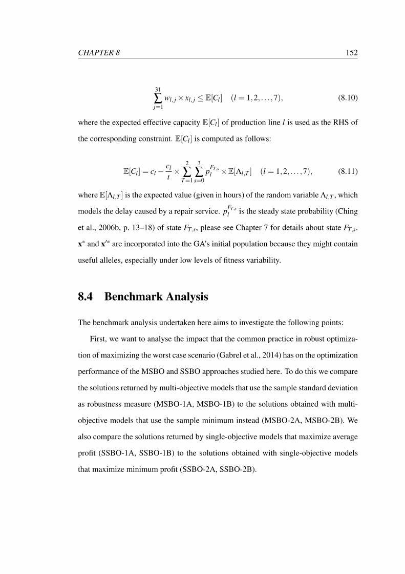
CHAPTER 8 152
31
∑j=1
wl, j× xl, j ≤ E[Cl] (l = 1,2, . . . ,7), (8.10)
where the expected effective capacity E[Cl] of production line l is used as the RHS of
the corresponding constraint. E[Cl] is computed as follows:
E[Cl] = cl−cl
t×
2
∑T=1
3
∑s=0
pFT,sl ×E[Λl,T ] (l = 1,2, . . . ,7), (8.11)
where E[Λl,T ] is the expected value (given in hours) of the random variable Λl,T , which
models the delay caused by a repair service. pFT,sl is the steady state probability (Ching
et al., 2006b, p. 13–18) of state FT,s, please see Chapter 7 for details about state FT,s.
x∗ and x′∗ are incorporated into the GA’s initial population because they might contain
useful alleles, especially under low levels of fitness variability.
8.4 Benchmark Analysis
The benchmark analysis undertaken here aims to investigate the following points:
First, we want to analyse the impact that the common practice in robust optimiza-
tion of maximizing the worst case scenario (Gabrel et al., 2014) has on the optimization
performance of the MSBO and SSBO approaches studied here. To do this we compare
the solutions returned by multi-objective models that use the sample standard deviation
as robustness measure (MSBO-1A, MSBO-1B) to the solutions obtained with multi-
objective models that use the sample minimum instead (MSBO-2A, MSBO-2B). We
also compare the solutions returned by single-objective models that maximize average
profit (SSBO-1A, SSBO-1B) to the solutions obtained with single-objective models
that maximize minimum profit (SSBO-2A, SSBO-2B).
CHAPTER 8 153
Second, we intend to investigate how the allocation of limited computations be-
tween refinement of fitness values and longer optimization runs affects the optimiza-
tion performance of the single and multi-objective models analysed, and whether the
impact of this differs between the different formulations. To do this we compare (for
every single and multi-objective model) two sets of solutions: the ones obtained when
fitness values are computed across 10 (explicit averaging strategy A) and 30 (explicit
averaging strategy B) fitness evaluations.
Third, we want to investigate to what extent ESO optimization is able to generate,
from a diverse final population, trade-off solutions between performance and robust-
ness by optimizing a single measure that implicitly considers robustness, and how this
compares to EMO optimization, where robustness is considered explicitly as an addi-
tional objective. To do this, we compare the solutions returned by the different single
and multi-objective models.
Finally, in order to understand how performance differences evolve with increasing
uncertainty levels across the different models analysed, we address the points men-
tioned above in two different problem instances, presented in Table 8.1. Table 8.1
shows the values assigned to pl , ζl , ϕl and µl,T , which are necessary to compute (as
shown in Chapter 7) the transition probability matrix of each production line for both
problem instances analysed in this study. pl is the probability that a production line
failure occurs (either serious or non-serious) during the manufacturing of the next prod-
uct lot, given that the production line is in state O0 (no non-serious failure has occurred
after a near-perfect repair and the production line was operative during the manufac-
turing of the current product lot). ζl determines the probability that a serious failure
occurs during the manufacturing of the next product lot, given that the production line
is in state O0 and given that a production line failure occurs during the manufacturing
of the next product lot. The deterioration of a production line caused by a non-serious
failure is modelled by raising pl and ζl to the power of ϕl . The random variable Λl,T
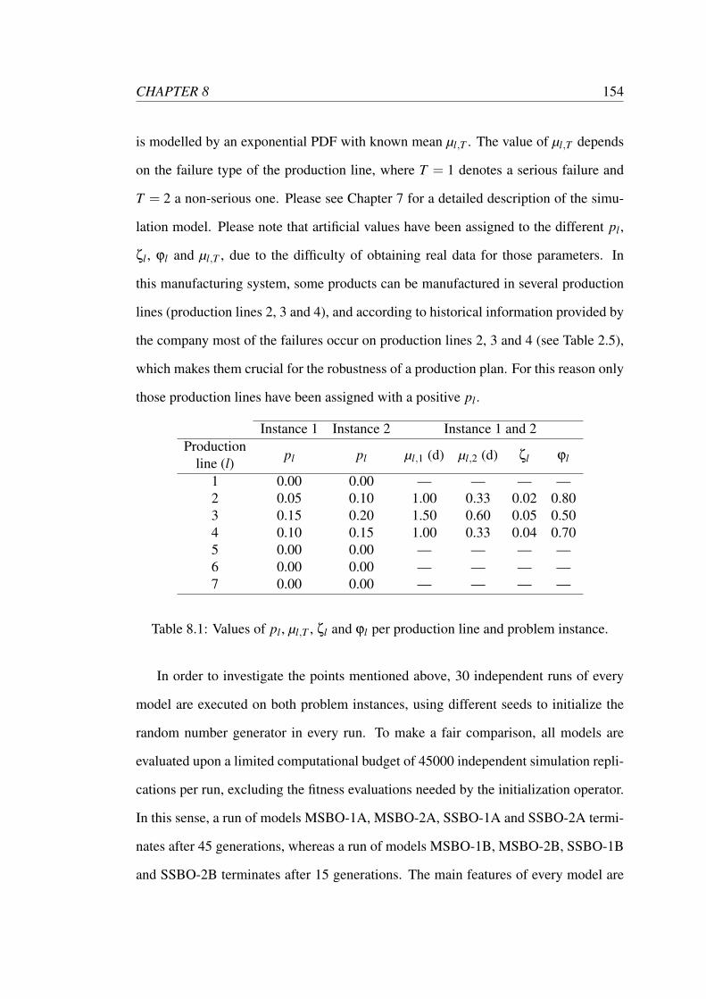
CHAPTER 8 154
is modelled by an exponential PDF with known mean µl,T . The value of µl,T depends
on the failure type of the production line, where T = 1 denotes a serious failure and
T = 2 a non-serious one. Please see Chapter 7 for a detailed description of the simu-
lation model. Please note that artificial values have been assigned to the different pl ,
ζl , ϕl and µl,T , due to the difficulty of obtaining real data for those parameters. In
this manufacturing system, some products can be manufactured in several production
lines (production lines 2, 3 and 4), and according to historical information provided by
the company most of the failures occur on production lines 2, 3 and 4 (see Table 2.5),
which makes them crucial for the robustness of a production plan. For this reason only
those production lines have been assigned with a positive pl .
Instance 1 Instance 2 Instance 1 and 2Production
pl pl µl,1 (d) µl,2 (d) ζl ϕlline (l)1 0.00 0.00 — — — —2 0.05 0.10 1.00 0.33 0.02 0.803 0.15 0.20 1.50 0.60 0.05 0.504 0.10 0.15 1.00 0.33 0.04 0.705 0.00 0.00 — — — —6 0.00 0.00 — — — —7 0.00 0.00 — — — —
Table 8.1: Values of pl , µl,T , ζl and ϕl per production line and problem instance.
In order to investigate the points mentioned above, 30 independent runs of every
model are executed on both problem instances, using different seeds to initialize the
random number generator in every run. To make a fair comparison, all models are
evaluated upon a limited computational budget of 45000 independent simulation repli-
cations per run, excluding the fitness evaluations needed by the initialization operator.
In this sense, a run of models MSBO-1A, MSBO-2A, SSBO-1A and SSBO-2A termi-
nates after 45 generations, whereas a run of models MSBO-1B, MSBO-2B, SSBO-1B
and SSBO-2B terminates after 15 generations. The main features of every model are
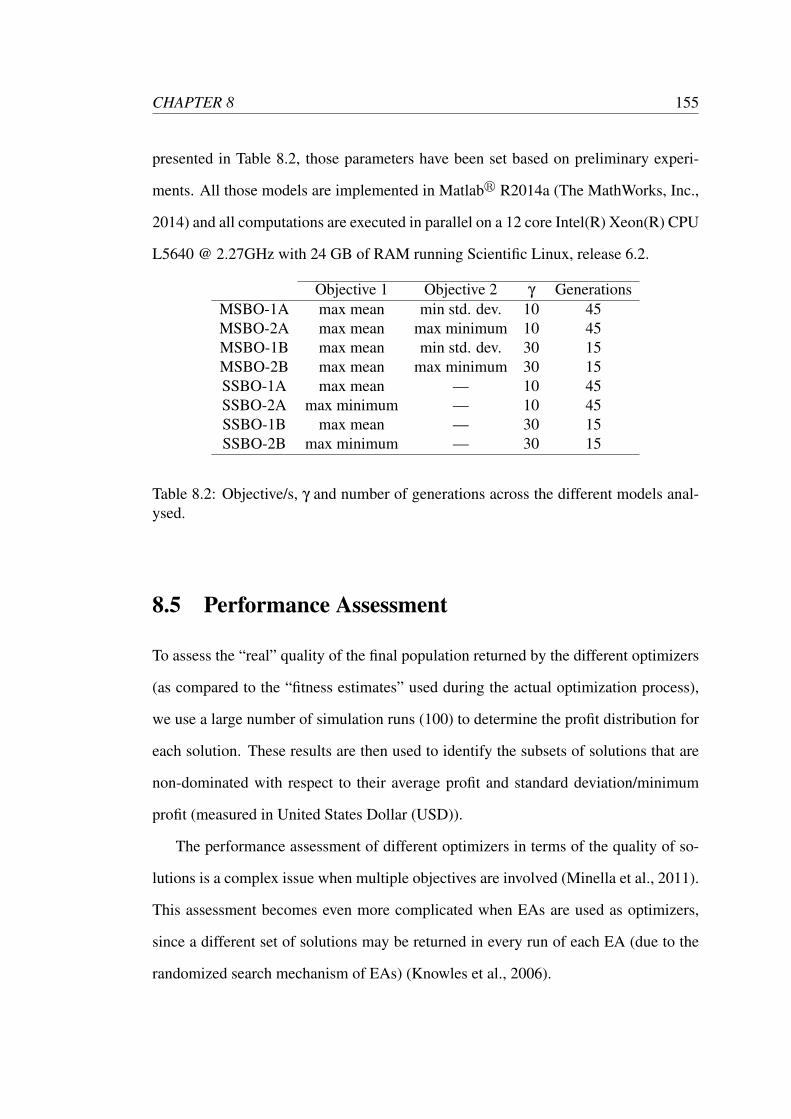
CHAPTER 8 155
presented in Table 8.2, those parameters have been set based on preliminary experi-
ments. All those models are implemented in Matlabr R2014a (The MathWorks, Inc.,
2014) and all computations are executed in parallel on a 12 core Intel(R) Xeon(R) CPU
L5640 @ 2.27GHz with 24 GB of RAM running Scientific Linux, release 6.2.
Objective 1 Objective 2 γ GenerationsMSBO-1A max mean min std. dev. 10 45MSBO-2A max mean max minimum 10 45MSBO-1B max mean min std. dev. 30 15MSBO-2B max mean max minimum 30 15SSBO-1A max mean — 10 45SSBO-2A max minimum — 10 45SSBO-1B max mean — 30 15SSBO-2B max minimum — 30 15
Table 8.2: Objective/s, γ and number of generations across the different models anal-ysed.
8.5 Performance Assessment
To assess the “real” quality of the final population returned by the different optimizers
(as compared to the “fitness estimates” used during the actual optimization process),
we use a large number of simulation runs (100) to determine the profit distribution for
each solution. These results are then used to identify the subsets of solutions that are
non-dominated with respect to their average profit and standard deviation/minimum
profit (measured in United States Dollar (USD)).
The performance assessment of different optimizers in terms of the quality of so-
lutions is a complex issue when multiple objectives are involved (Minella et al., 2011).
This assessment becomes even more complicated when EAs are used as optimizers,
since a different set of solutions may be returned in every run of each EA (due to the
randomized search mechanism of EAs) (Knowles et al., 2006).
CHAPTER 8 156
Different approaches to assess performance of multi-objective optimizers have been
proposed in the existing literature, the reader is referred to Knowles et al. (2006) for a
comprehensive review of existing techniques. Here, in order to evaluate the points of
interest mentioned at the beginning of this section (Section 8.4), we use the multiple
sets of non-dominated solutions obtained with every model (MSBO-1A, MSBO-1B,
MSBO-2A, MSBO-2B, SSBO-1A, SSBO-1B, SSBO-2A and SSBO-2B) to compute
samples of values for the hypervolume indicator (Fleischer, 2003). We then conduct
Mann-Whitney U tests (Mann and Whitney, 1947) on the samples of hypervolume
values in order to derive statistical inferences about the relative performance of two
models expressed in the form of the following hypotheses:
Ho : stochastic homogeneity of hypervolume values
Ha : stochastic heterogeneity of hypervolume values
In this sense, Mann-Whitney U tests tell us if one model outperforms other model
in terms of the quality of approximation sets generated, under the assumption that the
hypervolume indicator reflects the preference of the decision maker (Knowles et al.,
2006). A non-parametric test (Mann-Whitney U test) is employed because distribu-
tions of the samples analysed do not fulfil the normality assumption.
The use of the hypervolume indicator might favour multi-objective formulations
over single-objective formulations given that diversity is explicitly considered in the
former models, but not in the latter ones. In order to resolve this potential issue and
make a fair comparison between single and multi-objective models, we apply the at-
tainment function approach (da Fonseca and Fonseca, 2010; da Fonseca et al., 2001).
This approach summarizes the outcome of multiple runs of the different models in the
form of empirical attainment functions 2 (EAF) (Binois et al., 2015), and thus enable
2An attainment function describes the probability of an algorithm finding at least one solution whoseobjective vector dominates or is equal to a specific objective vector in a single run (da Fonseca et al.,2001; Fonseca and Fleming, 1996). The attainment function can be approximated from the outcomesof several independent runs of an algorithm, such approximation is known as the empirical attainmentfunction (Lopez-Ibanez et al., 2010)
CHAPTER 8 157
us to identify the region/s where performance differences arise between single and
multi-objective models, in both objective spaces analysed (i average profit vs. stan-
dard deviation of profit and ii average profit vs. minimum profit). We employ the eaf
package presented in Lopez-Ibanez et al. (2010) to create plots of the median (objec-
tive vectors attained by at least half of the runs) and best (best objective vector ever
achieved) attainment surfaces as well as to illustrate the differences between EAFs
obtained with different models.
8.6 Results
Yet, given that the sample minimum presents a biased estimator for the population (Lopez-
Ibanez et al., 2010), it is possible that its as a robustness measure may mislead selec-
tion operators and steer an EA towards undesirable regions of the objective space.
Our results provide evidence supporting the idea that the use of less biased statistics
as robustness measures reduces the computational effort needed to obtain reliable fit-
ness estimates, thus reducing the likelihood of choosing bad solutions over good ones
during the optimization and making it possible to allocate more computational effort
to the optimization procedure. This can be seen in results from Mann-Whitney U
tests (presented in Tables 8.3 and 8.4 for problem instance 1 and Tables 8.5 and 8.6
for problem instance 2 located Appendix 8.A), which statistically show that in both
objective spaces analysed (i average profit vs. standard deviation of profit and ii aver-
age profit vs. minimum profit) multi-objective models that used the sample standard
deviation as robustness measure (MSBO-1A and MSBO-1B) achieved stochastically
larger (p < .01) hypervolume values than their counterparts (MSBO-2A and MSBO-
2B) that used the sample minimum as robustness measure. Figures 8.1 and 8.2 also
support this finding in problem instance 1, by showing that the CDFs of hypervolume
values obtained with MSBO-2A and MSBO-2B are dominated (first and second-order
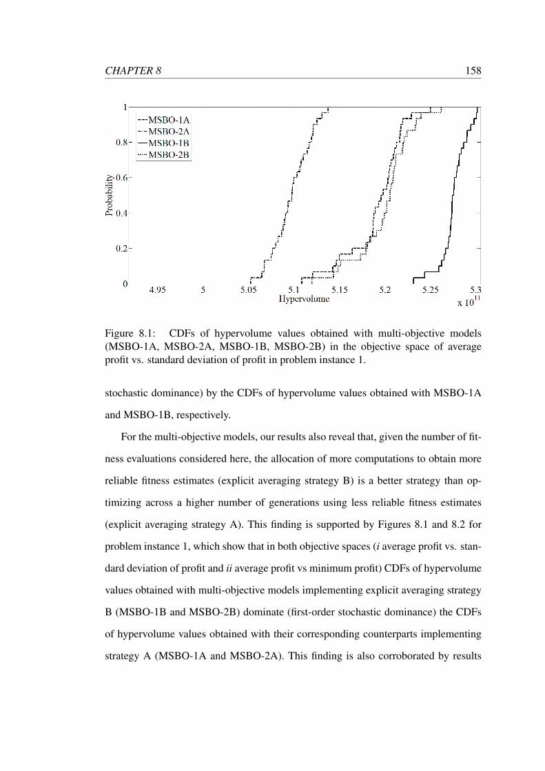
CHAPTER 8 158
Figure 8.1: CDFs of hypervolume values obtained with multi-objective models(MSBO-1A, MSBO-2A, MSBO-1B, MSBO-2B) in the objective space of averageprofit vs. standard deviation of profit in problem instance 1.
stochastic dominance) by the CDFs of hypervolume values obtained with MSBO-1A
and MSBO-1B, respectively.
For the multi-objective models, our results also reveal that, given the number of fit-
ness evaluations considered here, the allocation of more computations to obtain more
reliable fitness estimates (explicit averaging strategy B) is a better strategy than op-
timizing across a higher number of generations using less reliable fitness estimates
(explicit averaging strategy A). This finding is supported by Figures 8.1 and 8.2 for
problem instance 1, which show that in both objective spaces (i average profit vs. stan-
dard deviation of profit and ii average profit vs minimum profit) CDFs of hypervolume
values obtained with multi-objective models implementing explicit averaging strategy
B (MSBO-1B and MSBO-2B) dominate (first-order stochastic dominance) the CDFs
of hypervolume values obtained with their corresponding counterparts implementing
strategy A (MSBO-1A and MSBO-2A). This finding is also corroborated by results
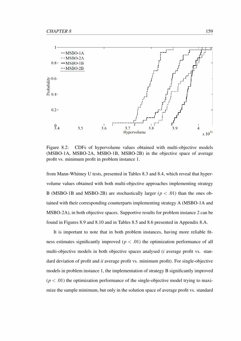
CHAPTER 8 159
Figure 8.2: CDFs of hypervolume values obtained with multi-objective models(MSBO-1A, MSBO-2A, MSBO-1B, MSBO-2B) in the objective space of averageprofit vs. minimum profit in problem instance 1.
from Mann-Whitney U tests, presented in Tables 8.3 and 8.4, which reveal that hyper-
volume values obtained with both multi-objective approaches implementing strategy
B (MSBO-1B and MSBO-2B) are stochastically larger (p < .01) than the ones ob-
tained with their corresponding counterparts implementing strategy A (MSBO-1A and
MSBO-2A), in both objective spaces. Supportive results for problem instance 2 can be
found in Figures 8.9 and 8.10 and in Tables 8.5 and 8.6 presented in Appendix 8.A.
It is important to note that in both problem instances, having more reliable fit-
ness estimates significantly improved (p < .01) the optimization performance of all
multi-objective models in both objective spaces analysed (i average profit vs. stan-
dard deviation of profit and ii average profit vs. minimum profit). For single-objective
models in problem instance 1, the implementation of strategy B significantly improved
(p < .01) the optimization performance of the single-objective model trying to maxi-
mize the sample minimum, but only in the solution space of average profit vs. standard
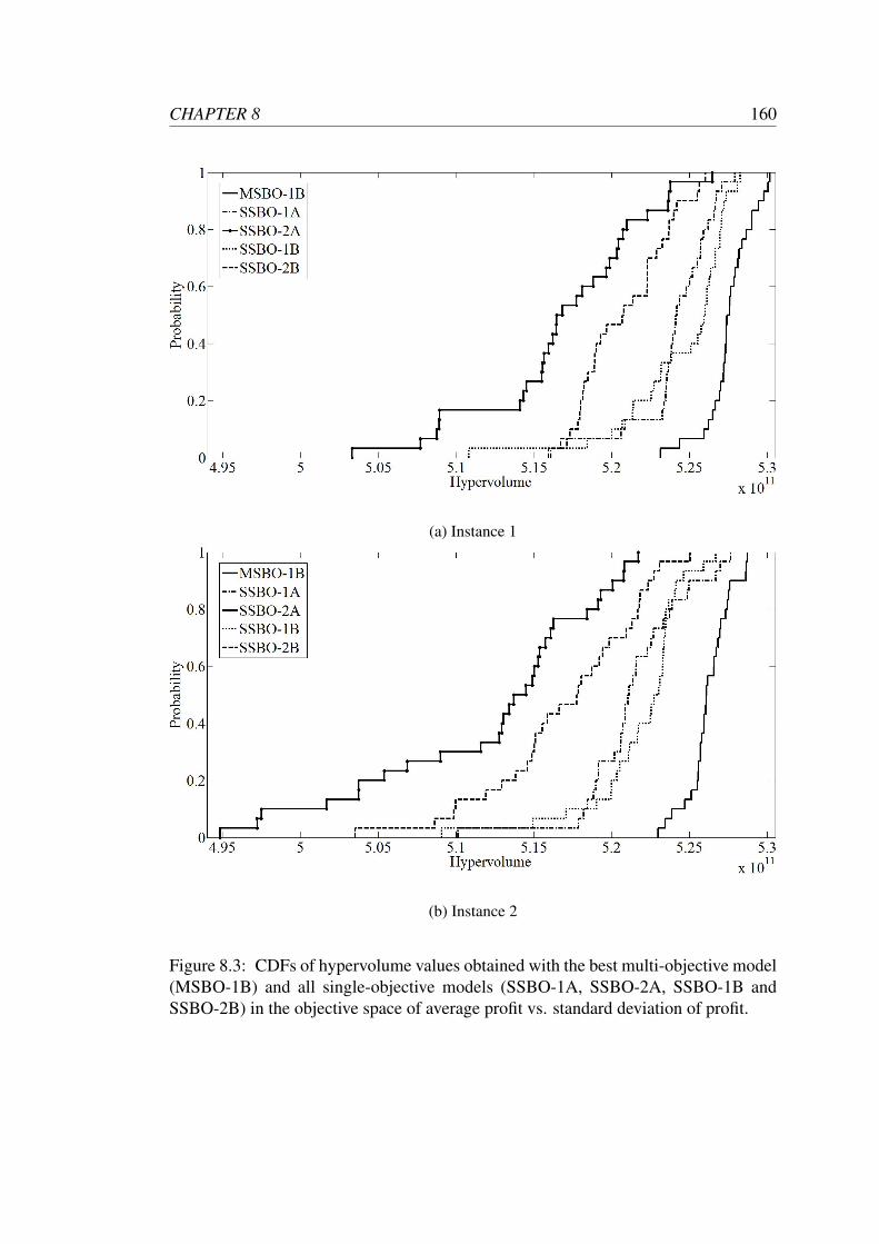
CHAPTER 8 160
(a) Instance 1
(b) Instance 2
Figure 8.3: CDFs of hypervolume values obtained with the best multi-objective model(MSBO-1B) and all single-objective models (SSBO-1A, SSBO-2A, SSBO-1B andSSBO-2B) in the objective space of average profit vs. standard deviation of profit.
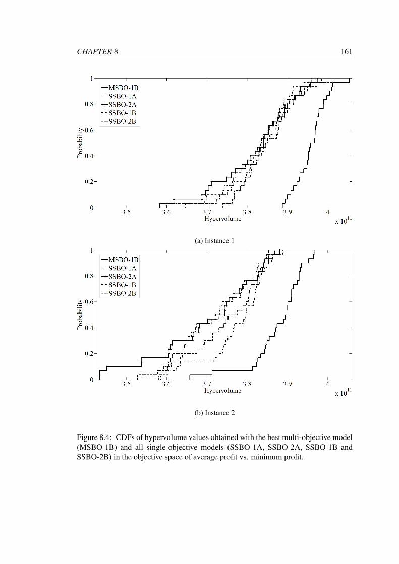
CHAPTER 8 161
(a) Instance 1
(b) Instance 2
Figure 8.4: CDFs of hypervolume values obtained with the best multi-objective model(MSBO-1B) and all single-objective models (SSBO-1A, SSBO-2A, SSBO-1B andSSBO-2B) in the objective space of average profit vs. minimum profit.
CHAPTER 8 162
deviation (see Table 8.3 and 8.5, where SSBO-2B achieved stochastically larger hy-
pervolume values (p < .01) than SSBO-2A), whereas under higher uncertainty level
(problem instance 2), strategy B improved the optimization performance of the model
mentioned above not only in the solution space of average profit vs. standard devi-
ation, but also in the solution space of average profit vs. minimum profit (see Fig-
ures 8.3b and 8.4b, where the CDF of hypervolume values obtained with SSBO-2B
dominate the CDFs of hypervolume values obtained with SSBO-2A - first and second-
order stochastic dominance, respectively). These results are interesting because they
provide evidence that using less biased statistics as objective/s might reduce the com-
putational effort (number of samples) needed to obtain reliable fitness estimates, and
thus demonstrate that not only the level of uncertainty, but also the choice of objec-
tive/s have an impact on the noise sensitivity of the optimization approach. Our results
also seem to suggest that the multi-objective approach is more sensitive to noise than
the single-objective approach, but further investigation is still required to support this
claim. This may occur because in the single-objective case the solution selection dur-
ing the optimization procedure only considers one noisy fitness estimate, whereas in
the multi-objective case the noise affecting the optimization comes from two different
noisy fitness estimates, which makes the solution selection more difficult. Although
we cannot claim that multi-objective approaches are in general more noise sensitive
than the single-objective approaches, as this will highly depend on the choice of objec-
tive/s, we can say that our experiments demonstrate that for the multi-objective models
considered here, allocating more computational effort towards the generation of more
reliable fitness estimates seems to be more beneficial than optimizing across more gen-
erations.
Our results identified MSBO-1B as the best multi-objective model in both objective
spaces analysed in problem instance 1 and 2. In the solution space of average profit vs.
standard deviation of profit, this finding is confirmed by results from Mann-Whitney
CHAPTER 8 163
U tests (Tables 8.3 and 8.5) and by analysing Figures 8.1 and 8.9, which indicate
that MSBO-1B outperformed all its multi-objective contestants (MSBO-1A, MSBO-
2A and MSBO-2B). Furthermore, hypervolume values from non-dominated solutions
found with MSBO-1B in the solution space of average profit vs. minimum profit were
stochastically larger (p < .01) (see Tables 8.4 and 8.6) than hypervolume values ob-
tained with any other multi-objective model (MSBO-1A, MSBO-2A and MSBO-2B),
in both problem instances. For problem instance 1, these results are corroborated by
Figure 8.2, where the CDF of hypervolume values obtained with MSBO-1B domi-
nates the CDFs obtained with MSBO-1A (first-order stochastic dominance), MSBO-
2A (first-order stochastic dominance) and MSBO-2B (second-order stochastic domi-
nance).
It is not surprising that MSBO-1B outperforms both, MSBO-2A and MSBO-2B,
in the solution space of average profit vs. standard deviation of profit, since MSBO-1B
explicitly optimizes both criteria. However, it is surprising that MSBO-1B also outper-
forms MSBO-2A and MSBO-2B in the solution space of average profit vs. minimum
profit, considering that maximization of minimum profit is an objective in MSBO-2A
and MSBO-2B, but not in MSBO-1B. This counter-intuitive result further supports our
finding that the use of the sample minimum as robustness measure may undermine the
optimization performance of the EAs analysed, instead of returning more robust so-
lutions, as reported in Ong et al. (2006) and Tsutsui (1999), compared to less biased
statistics such as the sample mean or the sample standard deviation. Having a more
biased statistic (sample minimum) as one of the two noisy fitness estimates may be the
reason why MSBO-2B was outperformed in both objective spaces (based on CDFs and
results from Mann-Whitney U tests) by MSBO-1B, which uses a less biased statistic
(sample standard deviation) as fitness estimate. It is probably due to the less reliable
fitness estimates that MSBO-1A performed so badly (based on CDFs and results from
CHAPTER 8 164
Mann-Whitney U tests) in both objective spaces in terms of hypervolume values com-
pared to MSBO-1B, which has more refined fitness estimates.
Our results also demonstrate that the simultaneous optimization of average profit
as a performance measure and standard deviation of profit as a robustness measure
(MSBO-1B) consistently generated better sets of trade-off solutions not only between
average profit and standard deviation of profit, but also between average profit and
minimum profit, than any other model here analysed. The supporting evidence for
this finding is provided by results from Mann-Whitney U tests (Tables 8.3 and 8.4 for
problem instance 1 and Tables 8.5 and 8.6 for problem instance 2), which determined
that MSBO-1B achieved stochastically larger (p < .01) hypervolume values than any
of the single-objective models in both objective spaces analysed. The superiority of
MSBO-1B is also illustrated in Figures 8.3 and 8.4, where the CDFs of hypervolume
values obtained with MSBO-1B dominate (first-order stochastic dominance) all the
CDFs obtained with the single-objective models (SSBO-1A, SSBO-2A, SSBO-1B and
SSBO-2B).
Finally, the median and best attainment surfaces, presented in Figures 8.5, 8.6, 8.7
and 8.8, illustrate that in problem instance 1 and 2, respectively, the regions attained
in both objective spaces with the best multi-objective model (MSBO-1B) are more
attractive than the ones attained with the different single-objective models (SSBO-
1A, SSBO-2A, SSBO-1B and SSBO-2B). The advantage of MSBO-1B over single-
objective models is also confirmed by looking at the shaded areas in those figures.
Shaded areas point out the regions of the objective space where the EAF of one model
is larger by at least 20% than the EAF of the other model, and thus dark regions in-
dicate the location in the objective space where one model outperformed the other.
Darker areas indicate larger differences between the estimated probability values of
two models.
This finding is somewhat surprising when considering performance for one of the
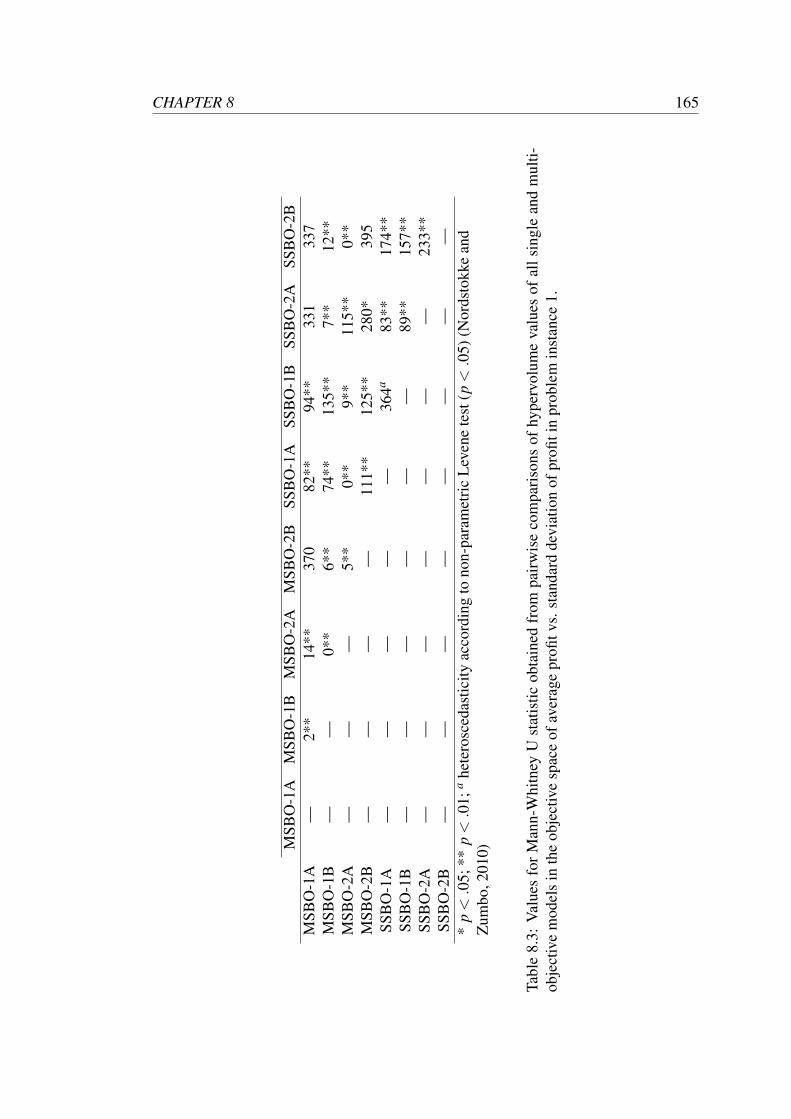
CHAPTER 8 165
MSB
O-1
AM
SBO
-1B
MSB
O-2
AM
SBO
-2B
SSB
O-1
ASS
BO
-1B
SSB
O-2
ASS
BO
-2B
MSB
O-1
A—
2**
14**
370
82**
94**
331
337
MSB
O-1
B—
—0*
*6*
*74
**13
5**
7**
12**
MSB
O-2
A—
——
5**
0**
9**
115*
*0*
*M
SBO
-2B
——
——
111*
*12
5**
280*
395
SSB
O-1
A—
——
——
364a
83**
174*
*SS
BO
-1B
——
——
——
89**
157*
*SS
BO
-2A
——
——
——
—23
3**
SSB
O-2
B—
——
——
——
—*
p<.0
5;**
p<.0
1;a
hete
rosc
edas
ticity
acco
rdin
gto
non-
para
met
ric
Lev
ene
test
(p<.0
5)(N
ords
tokk
ean
dZ
umbo
,201
0)
Tabl
e8.
3:V
alue
sfo
rM
ann-
Whi
tney
Ust
atis
ticob
tain
edfr
ompa
irw
ise
com
pari
sons
ofhy
perv
olum
eva
lues
ofal
lsin
gle
and
mul
ti-ob
ject
ive
mod
els
inth
eob
ject
ive
spac
eof
aver
age
profi
tvs.
stan
dard
devi
atio
nof
profi
tin
prob
lem
inst
ance
1.
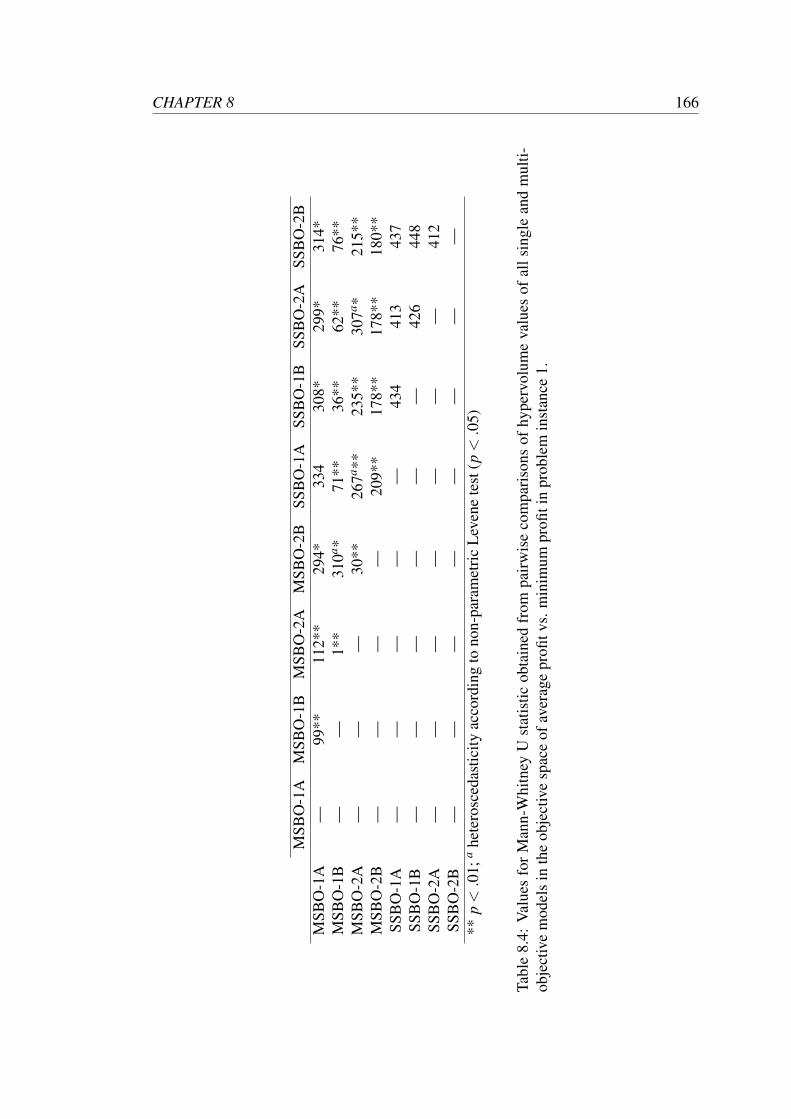
CHAPTER 8 166
MSB
O-1
AM
SBO
-1B
MSB
O-2
AM
SBO
-2B
SSB
O-1
ASS
BO
-1B
SSB
O-2
ASS
BO
-2B
MSB
O-1
A—
99**
112*
*29
4*33
430
8*29
9*31
4*M
SBO
-1B
——
1**
310a *
71**
36**
62**
76**
MSB
O-2
A—
——
30**
267a **
235*
*30
7a *21
5**
MSB
O-2
B—
——
—20
9**
178*
*17
8**
180*
*SS
BO
-1A
——
——
—43
441
343
7SS
BO
-1B
——
——
——
426
448
SSB
O-2
A—
——
——
——
412
SSB
O-2
B—
——
——
——
—**
p<.0
1;a
hete
rosc
edas
ticity
acco
rdin
gto
non-
para
met
ric
Lev
ene
test
(p<.0
5)
Tabl
e8.
4:V
alue
sfo
rM
ann-
Whi
tney
Ust
atis
ticob
tain
edfr
ompa
irw
ise
com
pari
sons
ofhy
perv
olum
eva
lues
ofal
lsin
gle
and
mul
ti-ob
ject
ive
mod
els
inth
eob
ject
ive
spac
eof
aver
age
profi
tvs.
min
imum
profi
tin
prob
lem
inst
ance
1.
CHAPTER 8 167
extremes of the (approximated) Pareto front (e.g. high average profit, high minimum
profit): as the single-objective optimizer is focusing on the optimization of a specific
criterion, we may expect it to outperform the multi-objective optimizer in the corre-
sponding region of the front. However, this does not occur. This appears to indicate
that the simultaneous consideration of multiple objectives allows for a more compre-
hensive description (and recognition) of good solutions during the optimization: the
solutions identified by the multi-objective approach “stand up” to the scrutiny of 100
simulations during final performance assessment, while the single-objective solutions
“drop” in performance.
8.7 Conclusion
As may be expected, our results suggest that a dedicated multi-objective approach is
able to consistently generate sets of solutions that present better trade-offs between per-
formance and robustness than a single-objective approach. More surprisingly though,
we observe that the single-objective models do not outperform the multi-objective ones
in extreme regions of the Pareto front, indicating that the multi-objective approach is
able to benefit from a more comprehensive description of solution quality.
We further establish that optimization performance for this problem is significantly
affected by the choice of robustness measure. In particular, the use of the sample
minimum as the robustness measure negatively impacts on the quality of the final so-
lutions, for both single-objective and multi-objective optimizers. In conjunction with
our experiments with sample size, we find that a larger number of evaluation replicates
(i.e. more computational effort) is needed to obtain reliable estimates for this measure,
compared to less biased statistics such as the sample mean or the sample standard
deviation.
While our results for the multi-objective optimizers are generally positive, we do
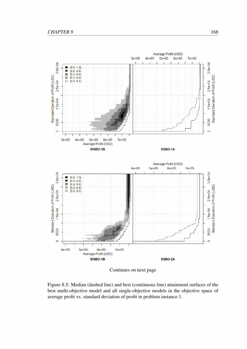
CHAPTER 8 168
Continues on next page
Figure 8.5: Median (dashed line) and best (continuous line) attainment surfaces of thebest multi-objective model and all single-objective models in the objective space ofaverage profit vs. standard deviation of profit in problem instance 1.
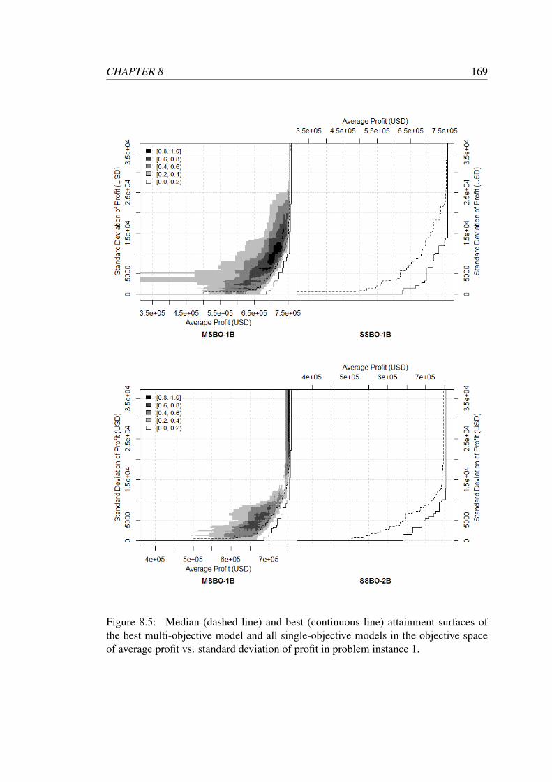
CHAPTER 8 169
Figure 8.5: Median (dashed line) and best (continuous line) attainment surfaces ofthe best multi-objective model and all single-objective models in the objective spaceof average profit vs. standard deviation of profit in problem instance 1.
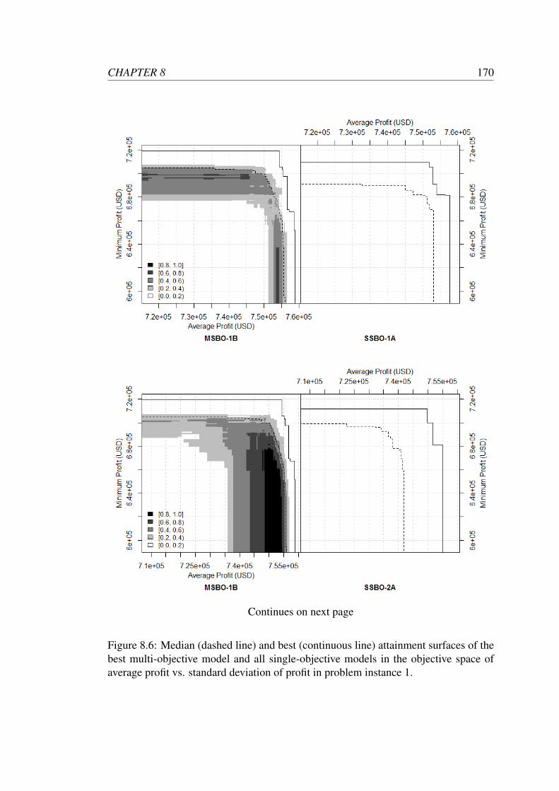
CHAPTER 8 170
Continues on next page
Figure 8.6: Median (dashed line) and best (continuous line) attainment surfaces of thebest multi-objective model and all single-objective models in the objective space ofaverage profit vs. standard deviation of profit in problem instance 1.
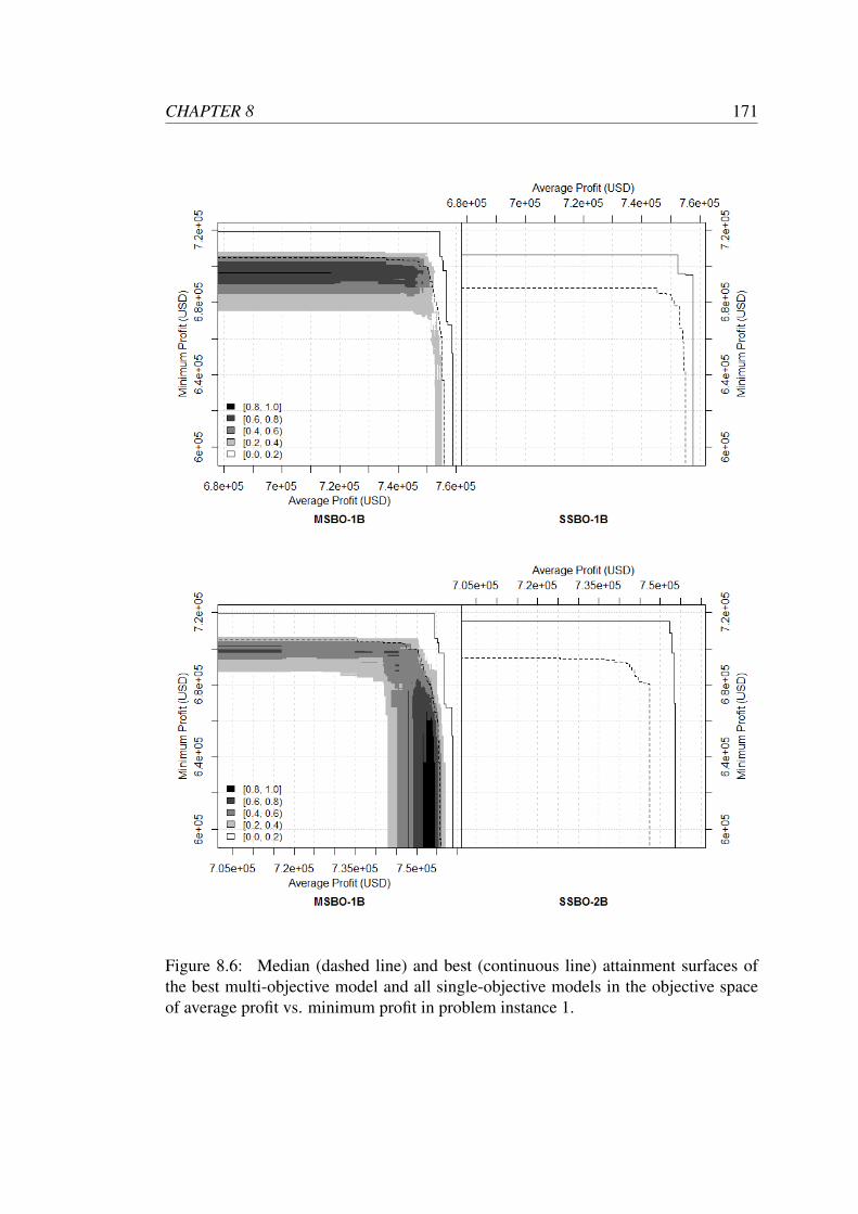
CHAPTER 8 171
Figure 8.6: Median (dashed line) and best (continuous line) attainment surfaces ofthe best multi-objective model and all single-objective models in the objective spaceof average profit vs. minimum profit in problem instance 1.
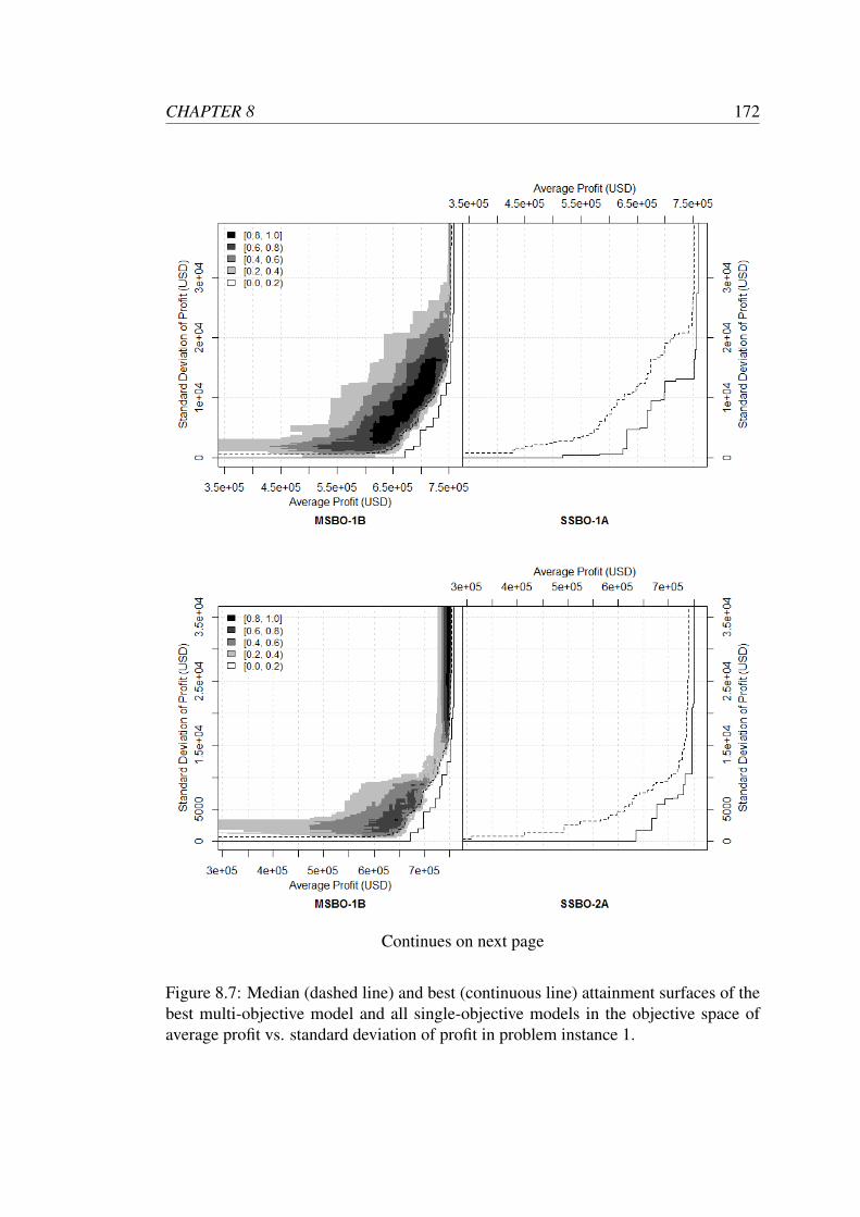
CHAPTER 8 172
Continues on next page
Figure 8.7: Median (dashed line) and best (continuous line) attainment surfaces of thebest multi-objective model and all single-objective models in the objective space ofaverage profit vs. standard deviation of profit in problem instance 1.
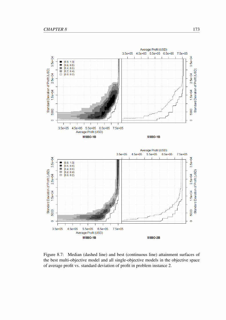
CHAPTER 8 173
Figure 8.7: Median (dashed line) and best (continuous line) attainment surfaces ofthe best multi-objective model and all single-objective models in the objective spaceof average profit vs. standard deviation of profit in problem instance 2.
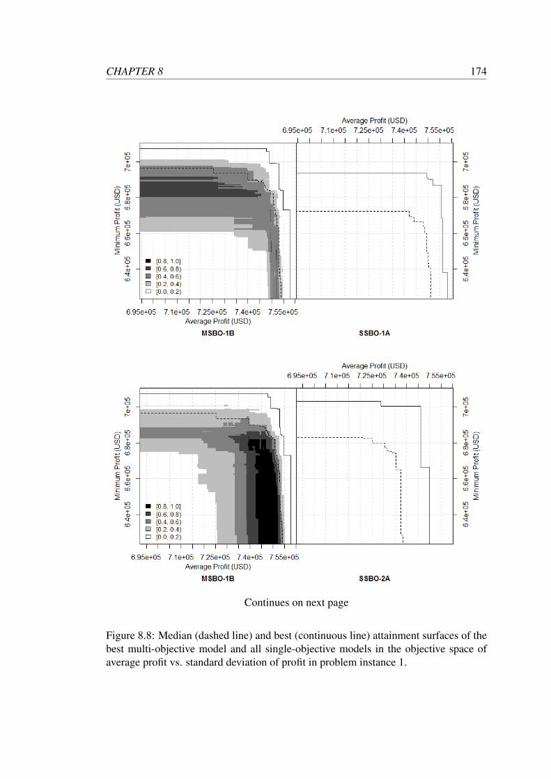
CHAPTER 8 174
Continues on next page
Figure 8.8: Median (dashed line) and best (continuous line) attainment surfaces of thebest multi-objective model and all single-objective models in the objective space ofaverage profit vs. standard deviation of profit in problem instance 1.
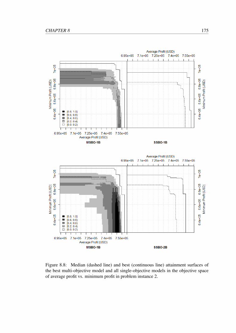
CHAPTER 8 175
Figure 8.8: Median (dashed line) and best (continuous line) attainment surfaces ofthe best multi-objective model and all single-objective models in the objective spaceof average profit vs. minimum profit in problem instance 2.

CHAPTER 8 176
identify a sensitivity of this approach to the number of evaluation replicates employed
in estimating fitness values, which highlights the importance of carefully adjusting
this parameter in multi-objective formulations for similar problems. In particular, our
results show that an increase in sample size (from 10 to 30) leads to a distinct per-
formance improvement for all multi-objective models, while this effect is much less
pronounced for the comparable single-objective models. We speculate that this may
be due to the simultaneous impact of noise in two objectives.
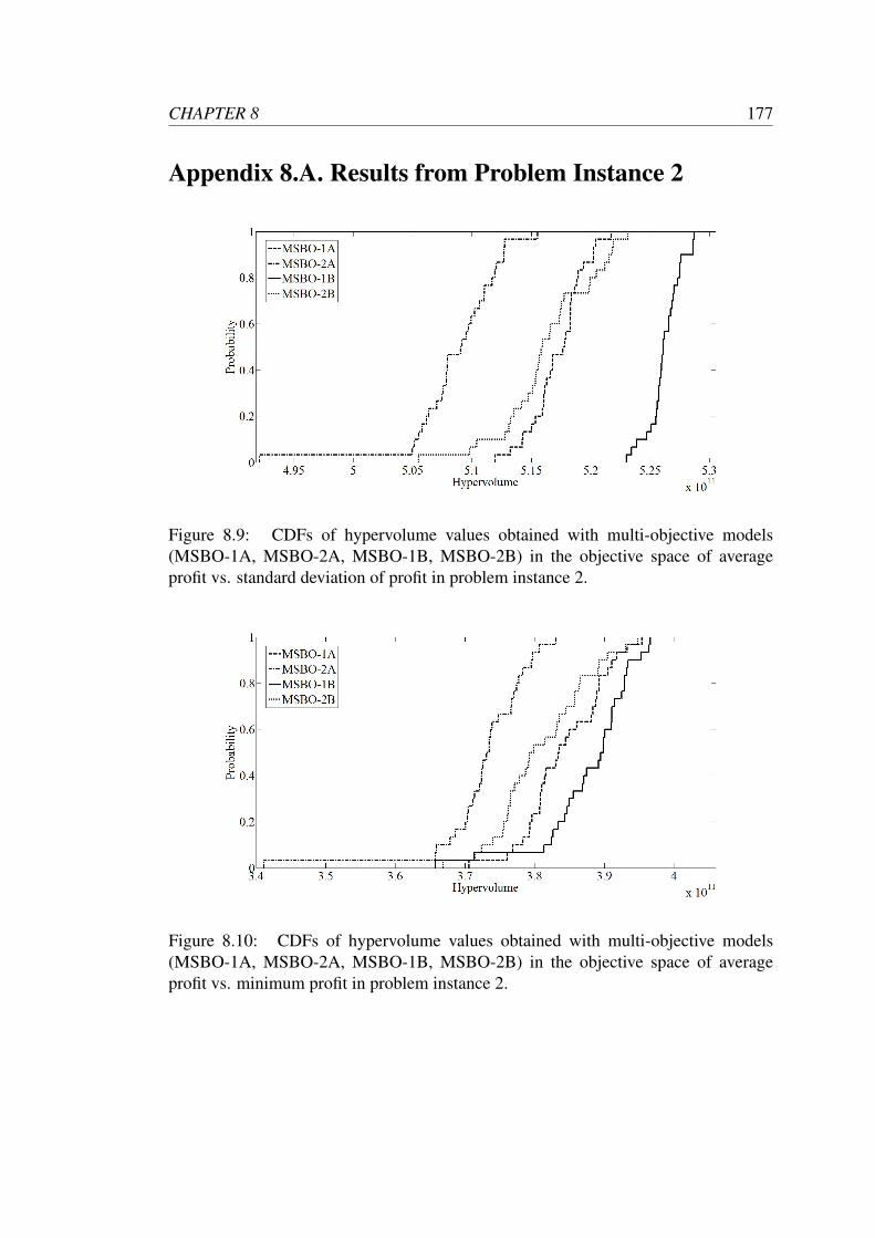
CHAPTER 8 177
Appendix 8.A. Results from Problem Instance 2
Figure 8.9: CDFs of hypervolume values obtained with multi-objective models(MSBO-1A, MSBO-2A, MSBO-1B, MSBO-2B) in the objective space of averageprofit vs. standard deviation of profit in problem instance 2.
Figure 8.10: CDFs of hypervolume values obtained with multi-objective models(MSBO-1A, MSBO-2A, MSBO-1B, MSBO-2B) in the objective space of averageprofit vs. minimum profit in problem instance 2.
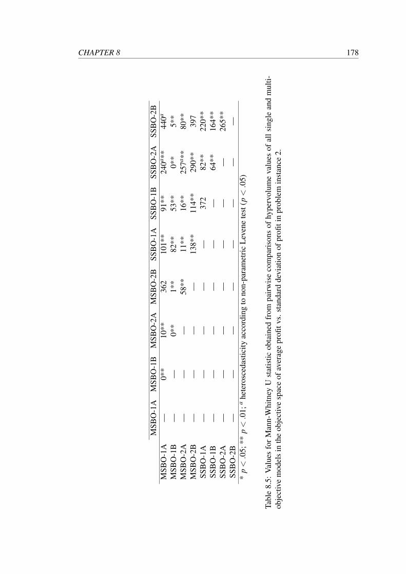
CHAPTER 8 178
MSB
O-1
AM
SBO
-1B
MSB
O-2
AM
SBO
-2B
SSB
O-1
ASS
BO
-1B
SSB
O-2
ASS
BO
-2B
MSB
O-1
A—
0**
10**
362
101*
*91
**24
0a **44
0a
MSB
O-1
B—
—0*
*1*
*82
**53
**0*
*5*
*M
SBO
-2A
——
—58
**11
**16
**25
7a **80
**M
SBO
-2B
——
——
138*
*11
4**
290*
*39
7SS
BO
-1A
——
——
—37
282
**22
0**
SSB
O-1
B—
——
——
—64
**16
4**
SSB
O-2
A—
——
——
——
265*
*SS
BO
-2B
——
——
——
——
*p<.0
5;**
p<.0
1;a
hete
rosc
edas
ticity
acco
rdin
gto
non-
para
met
ric
Lev
ene
test
(p<.0
5)
Tabl
e8.
5:V
alue
sfo
rM
ann-
Whi
tney
Ust
atis
ticob
tain
edfr
ompa
irw
ise
com
pari
sons
ofhy
perv
olum
eva
lues
ofal
lsin
gle
and
mul
ti-ob
ject
ive
mod
els
inth
eob
ject
ive
spac
eof
aver
age
profi
tvs.
stan
dard
devi
atio
nof
profi
tin
prob
lem
inst
ance
2.

CHAPTER 8 179
MSB
O-1
AM
SBO
-1B
MSB
O-2
AM
SBO
-2B
SSB
O-1
ASS
BO
-1B
SSB
O-2
ASS
BO
-2B
MSB
O-1
A—
264*
*62
**31
3**
127*
*23
8**
135*
*17
3**
MSB
O-1
B—
—52
**19
4**
62**
105*
*76
**79
**M
SBO
-2A
——
—16
4**
419a
241*
*42
7a36
1a
MSB
O-2
B—
——
—20
9**
360
215*
*27
5**
SSB
O-1
A—
——
——
295*
*43
738
0SS
BO
-1B
——
——
——
300*
*36
3SS
BO
-2A
——
——
——
—37
6SS
BO
-2B
——
——
——
——
**p<.0
1;a
hete
rosc
edas
ticity
acco
rdin
gto
non-
para
met
ric
Lev
ene
test
(p<.0
5)
Tabl
e8.
6:V
alue
sfo
rM
ann-
Whi
tney
Ust
atis
ticob
tain
edfr
ompa
irw
ise
com
pari
sons
ofhy
perv
olum
eva
lues
ofal
lsin
gle
and
mul
ti-ob
ject
ive
mod
els
inth
eob
ject
ive
spac
eof
aver
age
profi
tvs.
min
imum
profi
tin
prob
lem
inst
ance
2.
Chapter 9
Conclusion
Throughout this doctoral thesis we have investigated SBO as an alternative to conven-
tional optimization approaches to address real-world production planning problems,
where uncertainty and complexity are inherent features. We demonstrate that, for the
real-world production planning problem analysed in Chapter 5, both of our SBO ap-
proaches outperform two exact optimization techniques commonly applied in produc-
tion planning, namely ILP and CCP. We do not only provide concrete evidence of the
poor performance of those two exact techniques, but more importantly we demonstrate
that ILP and CCP can be used to significantly improve the optimization performance
of our SBO approach. More specifically, we illustrate that the implementation of spe-
cialized initialization operators that draw upon the solutions returned by ILP and CCP
combined with DES in a variety of ways is able to significantly improve the optimiza-
tion performance of a standard GA. This is an important finding that not only shows
the advantages of SBO approaches, but also highlights the synergies resulting from
the combination of population-based meta-heuristics with mathematical programming
methods. The use of specialized initialization operators to partially initialize the GA
population can be seen as a form of matheuristic (Villegas et al., 2013). Matheuristic
approaches are a relatively new area of research that is capturing the attention of a
180
CHAPTER 9 181
growing research community (Boschetti et al., 2009) due to its potential.
In Chapter 6, we further demonstrate the potential of matheuristics by implement-
ing an approach where all unfeasible solutions are removed from the search space.
In this approach a GA searches for capacity values of failure-prone production lines,
rather than directly searching for possible production plans. ILP in this approach acts
as a translation tool able to map every solution given by the GA onto a production plan.
Our specialized initialization operators from Chapter 5 and the matheuristic optimizer
proposed in Chapter 6 offer an opportunity to reduce the computational requirement
of EAs working in black-box optimization settings, which according to Coello (2006)
is an essential issue that deserves further investigation. We also introduce (Chapter 5)
an effective repair operator, which employs simulation to repair solutions that violate
capacity constraints, and propose a procedure based on explicit averaging (Jin and
Branke, 2005) to support the final solution selection of ESO (Chapters 4 and 5) and
EMO algorithms (Chapter 8).
In Chapter 8, we provide evidence for the advantages of a multi-objective formu-
lation over a single-objective formulation within the context of robust optimization.
Concretely, we illustrate that, for the real-world problem analysed, single-objective
approaches are limited in their ability to steer the search towards optimal trade-off so-
lutions between solution quality and robustness. As may be expected and suggested
in previous studies (Jin and Sendhoff, 2003), an explicit consideration of robustness
in the form of an additional objective proved to be a better alternative than optimizing
for a single objective that implicitly considers robustness (e.g. sample mean, sample
standard deviation or sample minimum). However, surprisingly our results also indi-
cate that the use of the sample minimum as a robustness measure has a detrimental
impact on the optimization performance of single and multi-objective formulations.
This may be because it increases the computational effort required to obtain reliable
estimates, compared to less biased statistics such as the sample mean or the sample
CHAPTER 9 182
standard deviation. This is a controversial finding, since some previous studies (Ong
et al., 2006; Tsutsui, 1999) have reported that more robust solutions can be obtained
by using the sample minimum as a robustness measure, and because the sample mini-
mum (worst case scenario for maximization problems) is a popular robustness measure
used in the search for robust solutions (Gabrel et al., 2014), some examples of this can
be found in Chen et al. (2016), Zhang et al. (2016), Goh and Tan (2007), Ong et al.
(2006) and Tsutsui (1999). Our experiments also seem to indicate that, in the context
of the problem analysed, multi-objective formulations may be more sensitive to noise
than single-objective formulations. This may occur because in the multi-objective case
the noise affecting the optimization comes from two different noisy fitness estimates,
which makes the solution selection more difficult than in the single-objective case,
where the solution selection only considers one noisy fitness estimate. For these rea-
sons, the choice of robustness measure and the sample size used during fitness evalua-
tion are essential considerations in designing a successful multi-objective approach for
robust optimization. Chapter 8 is focused on the interactions between the choice of op-
timization paradigm (multi-objective versus single-objective), robustness criterion and
sample size in the context of a production planning problem that is subject to machine
failures. This problem is an example of a much larger set of problems in which the
performance of a solution is subject to uncertainty in the operating or environmental
conditions (Lim et al., 2007, 2006; Jin and Branke, 2005).
In this thesis, we have aimed to illustrate the generality of our findings by proposing
general formulations of the problems analysed (Chapters 5, 6 and 8), by considering
results across a variety of uncertainty levels (Chapters 4, 5, 6 and 8) and by explor-
ing different levels of model complexity to model realistic features of manufacturing
systems (Chapter 7). Nevertheless, a remaining limitation of this doctoral thesis is the
fact that all of our experiments are performed in the context of a single real-world sys-
tem. Future research may therefore focus on validating the findings of this work in the
CHAPTER 9 183
context of different systems and different application areas.
We provide evidence that exact optimization techniques are limited in their ability
to accurately capture the complexity and uncertainty intrinsic to the real-world sys-
tem analysed (Chu et al., 2015; Guller et al., 2015). This is mainly because the level
of mathematical sophistication needed to model those complex features is no longer
within the framework of exact optimization techniques (Figueira and Almada-Lobo,
2014; Sel and Bilgen, 2014). Consequently, exact optimization techniques may need
to rely on overly stringent assumptions to cope with that complexity and keep the
problem computationally tractable (Gosavi, 2014, p. 31). However, the use of overly
stringent assumptions compromises the real applicability of solutions obtained (Niko-
lopoulou and Ierapetritou, 2012; Gnoni et al., 2003), basically because those are the
right solutions, but to the wrong problems. Therefore, we believe that the SBO ap-
proaches explored throughout this work may contribute to a wide range of real-world
applications, as we present some general ideas related to the incorporation of uncer-
tainty and complex features into the problem formulation as well as different solution
procedures that could be tailored to areas where mathematical programming methods
are being used to address problems where uncertainty is an inherent feature. Further-
more, the simultaneous consideration of tactical and operational decisions, e.g. having
the ability to re-optimize the problem after deviations have occurred, could further ex-
tend the applicability of our approaches to other areas. Stochastic programming with
recourse is an alternative worth exploring in this respect.
This thesis also provides general insights about the combined use of meta-heuristics
and exact optimization techniques. This combination of techniques is of particular in-
terest because of its potential to speed up convergence, which is utmost important when
function evaluations are expensive in terms of computational effort. Our experiments
suggest that when the problem formulation is beyond the framework of exact optimiza-
tion techniques, mathematical programming could be used to create initial solutions by
CHAPTER 9 184
solving a simplified formulation of the real problem, and then further improve those
initial solutions by applying meta-heuristic approaches that operate upon a more accu-
rate problem formulation. Given that evolutionary approaches are a common choice of
meta-heuristic, the development of specialized crossover and mutation operators able
to preserve the feasibility of solutions is an interesting avenue to improve the search
mechanism of those approaches. The design of feasibility-preserving operators would
be extremely useful to deal with constrained optimization problems, as turning good
solutions into unfeasible ones is one of the drawbacks of applying crossover or muta-
tion. Moreover, the elimination of unfeasible solutions from the search space by hav-
ing a meta-heuristic finding solutions in the genotypic search space and then applying
mathematical programming techniques to map a given genotype onto its phenotype
is also a promising alternative to deal with constrained optimization settings, espe-
cially when the problem formulation addressed by the exact optimization method is a
good approximation of the real problem. Finally, having an algorithm with the ability
to adapt its parameter values during the optimization is extremely important for the
case of meta-heuristics, where appropriate parameter tuning has a substantial impact
on algorithmic performance. Therefore, on-line parameter tuning is another interest-
ing topic that could be further explored towards the development of more effective
meta-heuristics, as this self-adaptation ability may cause substantial improvements in
the search mechanism and performance of the algorithm. For instance, it would be
advantageous to have a GA able to alter its mutation probability as well as the magni-
tude of those mutations along the path towards the optimum, as at the beginning of the
optimization big jumps might be beneficial (e.g. preventing getting trapped in local
optima), whereas at latter stages such big jumps might preclude finding the (global)
optimum.
Bibliography
F. Akhoondi and M. Lotfi. A heuristic algorithm for master production scheduling
problem with controllable processing times and scenario-based demands. Interna-
tional Journal of Production Research, pages 1–18, 2016.
R. Al-Aomar. Incorporating robustness into genetic algorithm search of stochastic sim-
ulation outputs. Simulation Modelling Practice and Theory, 14(3):201–223, 2006.
A. S. Alfa. Discrete-time markov chains. In Applied Discrete-Time Queues, pages
57–90. Springer, 2016.
C. Almeder and R. F. Hartl. A metaheuristic optimization approach for a real-world
stochastic flexible flow shop problem with limited buffer. International Journal of
Production Economics, 145(1):88–95, 2013.
C. Almeder, M. Preusser, and R. F. Hartl. Simulation and optimization of supply
chains: alternative or complementary approaches? OR spectrum, 31(1):95–119,
2009.
J. April, M. Better, F. Glover, J. Kelly, and M. Laguna. Enhancing business process
management with simulation optimization. In Proceedings of the 38th conference
on Winter simulation, pages 642–649. Winter Simulation Conference, 2006.
M. Arakawa, M. Fuyuki, and I. Inoue. An optimization-oriented method for
185
BIBLIOGRAPHY 186
simulation-based job shop scheduling incorporating capacity adjustment function.
International Journal of Production Economics, 85(3):359–369, 2003.
C. Azzaro-Pantel, L. Bernal-Haro, P. Baudet, S. Domenech, and L. Pibouleau. A two-
stage methodology for short-term batch plant scheduling: discrete-event simula-
tion and genetic algorithm. Computers & chemical engineering, 22(10):1461–1481,
1998.
S. Balev, N. Yanev, A. Frville, and R. Andonov. A dynamic programming based reduc-
tion procedure for the multidimensional 01 knapsack problem. European Journal of
Operational Research, 186(1):63–76, 2008.
E. B. Baum, D. Boneh, and C. Garrett. On genetic algorithms. In Proceedings of the
eighth annual conference on Computational learning theory, pages 230–239. ACM,
1995.
D. P. Bertsekas and J. N. Tsitsiklis. Introduction to Probability. Athena Scientific,
2008.
M. Bhattacharya, R. Islam, and A. N. Mahmood. Uncertainty and evolutionary opti-
mization: A novel approach. In Industrial Electronics and Applications (ICIEA),
2014 IEEE 9th Conference on, pages 988–993, June 2014.
M. Binois, D. Ginsbourger, and O. Roustant. Quantifying uncertainty on pareto fronts
with gaussian process conditional simulations. European Journal of Operational
Research, 243(2):386–394, 2015.
C. Blum and A. Roli. Hybrid metaheuristics: an introduction. In Hybrid Metaheuris-
tics, pages 1–30. Springer, 2008.
C. Blum, J. Puchinger, G. R. Raidl, and A. Roli. Hybrid metaheuristics in combinato-
rial optimization: A survey. Applied Soft Computing, 11(6):4135–4151, 2011.
BIBLIOGRAPHY 187
M. A. Boschetti, V. Maniezzo, M. Roffilli, and A. B. Rohler. Matheuristics: Optimiza-
tion, simulation and control. In Hybrid Metaheuristics, pages 171–177. Springer,
2009.
J. Branke. Creating robust solutions by means of evolutionary algorithms. In Parallel
Problem Solving from Nature PPSN V, pages 119–128. Springer, 1998.
J. Branke and K. Lu. Finding the trade-off between robustness and worst-case quality.
In Proceedings of the 2015 on Genetic and Evolutionary Computation Conference,
pages 623–630. ACM, 2015.
J. Branke and C. Schmidt. Selection in the presence of noise. In Genetic and Evolu-
tionary ComputationGECCO 2003, pages 766–777. Springer, 2003.
J. Branke, C. Schmidt, and H. Schmec. Efficient fitness estimation in noisy environ-
ments. In Proceedings of genetic and evolutionary computation. Citeseer, 2001.
J. Branke, S. Corrente, S. Greco, R. Słowinski, and P. Zielniewicz. Using choquet
integral as preference model in interactive evolutionary multiobjective optimization.
European Journal of Operational Research, 250(3):884–901, 2016.
A. E. Brownlee and J. A. Wright. Constrained, mixed-integer and multi-objective
optimisation of building designs by nsga-ii with fitness approximation. Applied Soft
Computing, 33(0):114–126, 2015.
E. K. Burke, T. Curtois, G. Kendall, M. Hyde, G. Ochoa, and J. A. Vazquez-Rodriguez.
Towards the decathlon challenge of search heuristics. In Proceedings of the 11th
Annual Conference Companion on Genetic and Evolutionary Computation Confer-
ence: Late Breaking Papers, pages 2205–2208. ACM, 2009.
M. Byrne and M. Bakir. Production planning using a hybrid simulation–analytical
approach. International Journal of Production Economics, 59(1):305–311, 1999.
BIBLIOGRAPHY 188
M. Byrne and M. Hossain. Production planning: An improved hybrid approach. Inter-
national Journal of Production Economics, 93:225–229, 2005.
M. Caserta and S. Voß. Metaheuristics: intelligent problem solving. In Matheuristics,
pages 1–38. Springer, 2009.
M. Caserta and S. Voß. A math-heuristic dantzig-wolfe algorithm for capacitated lot
sizing. Annals of Mathematics and Artificial Intelligence, 69(2):207–224, 2013.
A. Charnes and W. W. Cooper. Chance-constrained programming. Management sci-
ence, 6(1):73–79, 1959.
K. Chen and S. M. Ross. An adaptive stochastic knapsack problem. European Journal
of Operational Research, 239(3):625–635, 2014.
L. Chen, M. Gendreau, M. H. Ha, and A. Langevin. A robust optimization approach
for the road network daily maintenance routing problem with uncertain service time.
Transportation Research Part E: Logistics and Transportation Review, 85:40–51,
2016.
Y. Chen and J.-K. Hao. A reduce and solve approach for the multiple-choice multidi-
mensional knapsack problem. European Journal of Operational Research, 239(2):
313–322, 2014.
T.-m. Cheng and R.-z. Yan. Integrating messy genetic algorithms and simulation to op-
timize resource utilization. Computer-Aided Civil and Infrastructure Engineering,
24(6):401–415, 2009.
W.-K. Ching, X. Huang, M. K. Ng, and T.-K. Siu. Markov chains. Springer, 2006a.
W. K. Ching, X. Huang, M. K. Ng, and T.-K. Siu. Markov chains. Springer, 2006b.
BIBLIOGRAPHY 189
Y. Chu, F. You, J. M. Wassick, and A. Agarwal. Simulation-based optimization frame-
work for multi-echelon inventory systems under uncertainty. Computers & Chemi-
cal Engineering, 73(0):1–16, 2015.
C. A. C. Coello. Evolutionary multi-objective optimization: a historical view of the
field. Computational Intelligence Magazine, IEEE, 1(1):28–36, 2006.
C. A. C. Coello. Multi-objective evolutionary algorithms in real-world applications:
Some recent results and current challenges. In Advances in Evolutionary and De-
terministic Methods for Design, Optimization and Control in Engineering and Sci-
ences, pages 3–18. Springer, 2015.
J. B. Copas. Regression, prediction and shrinkage. Journal of the Royal Statistical
Society. Series B (Methodological), pages 311–354, 1983.
V. G. da Fonseca and C. M. Fonseca. The attainment-function approach to stochastic
multiobjective optimizer assessment and comparison. In Experimental methods for
the analysis of optimization algorithms, pages 103–130. Springer, 2010.
V. G. da Fonseca, C. M. Fonseca, and A. O. Hall. Inferential performance assessment
of stochastic optimisers and the attainment function. In Evolutionary multi-criterion
optimization, pages 213–225. Springer, 2001.
M. Dahane, N. Rezg, and A. Chelbi. Optimal production plan for a multi-products
manufacturing system with production rate dependent failure rate. International
Journal of Production Research, 50(13):3517–3528, 2012.
M. Dawande, J. Kalagnanam, P. Keskinocak, F. S. Salman, and R. Ravi. Approxi-
mation algorithms for the multiple knapsack problem with assignment restrictions.
Journal of combinatorial optimization, 4(2):171–186, 2000.
BIBLIOGRAPHY 190
B. C. Dean, M. X. Goemans, and J. Vondrak. Approximating the stochastic knapsack
problem: The benefit of adaptivity. Mathematics of Operations Research, 33(4):
945–964, 2008.
K. Deb. An efficient constraint handling method for genetic algorithms. Computer
methods in applied mechanics and engineering, 186(2):311–338, 2000.
K. Deb. Multi-objective optimization. In Search methodologies, pages 403–449.
Springer, 2014.
K. Deb and H. Gupta. Introducing robustness in multi-objective optimization. Evolu-
tionary Computation, 14(4):463–494, 2006.
K. Deb, A. Pratap, S. Agarwal, and T. Meyarivan. A fast and elitist multiobjective
genetic algorithm: Nsga-ii. Evolutionary Computation, IEEE Transactions on, 6(2):
182–197, 2002.
K. Deep and M. Thakur. A new crossover operator for real coded genetic algorithms.
Applied Mathematics and Computation, 188(1):895–911, 2007a.
K. Deep and M. Thakur. A new mutation operator for real coded genetic algorithms.
Applied mathematics and Computation, 193(1):211–230, 2007b.
K. Deep, K. P. Singh, M. Kansal, and C. Mohan. A real coded genetic algorithm for
solving integer and mixed integer optimization problems. Applied Mathematics and
Computation, 212(2):505–518, 2009.
J. E. Diaz and J. Handl. Simulation-based ga optimization for production planning.
In Bioinspired Optimization Methods and their Applications, pages 27–39. Jozef
Stefan Institute, 2014.
BIBLIOGRAPHY 191
J. E. Diaz and J. Handl. Implicit and explicit averaging strategies for simulation-
based optimization of a real-world production planning problem. Informatica: An
International Journal of Computing and Informatics, 39(2):161–168, 2015.
J. E. Diaz, J. Handl, and D.-L. Xu. Integrating meta-heuristics, simulation and exact
techniques for production planning of failure-prone manufacturing systems. Euro-
pean Journal of Operational Research, Submitted, 2015a.
J. E. Diaz, J. Handl, and D.-L. Xu. Single and multi-objective formulations for evolu-
tionary robust optimization - interaction between sample size and choice of robust-
ness measure. Computers & Operations Research, Submitted, 2015b.
M. Dıaz-Madronero, J. Mula, and D. Peidro. A review of discrete-time optimization
models for tactical production planning. International Journal of Production Re-
search, 52(17):5171–5205, 2014.
H. Ding, L. Benyoucef, and X. Xie. A simulation optimization methodology for sup-
plier selection problem. International Journal of Computer Integrated Manufactur-
ing, 18(2-3):210–224, 2005.
C. Ehrenberg and J. Zimmermann. Simulation-based optimization in make-to-order
production: scheduling for a special-purpose glass manufacturer. In Simulation
Conference (WSC), Proceedings of the 2012 Winter, pages 1–12. IEEE, 2012.
J. R. Evans. Applied production and operations management. West Publishing Com-
pany, 1990.
G. Figueira and B. Almada-Lobo. Hybrid simulation–optimization methods: A tax-
onomy and discussion. Simulation Modelling Practice and Theory, 46:118–134,
2014.
BIBLIOGRAPHY 192
M. Fleischer. The measure of pareto optima applications to multi-objective meta-
heuristics. In Evolutionary multi-criterion optimization, pages 519–533. Springer,
2003.
C. M. Fonseca and P. J. Fleming. On the performance assessment and comparison of
stochastic multiobjective optimizers. In Parallel problem solving from natureppsn
iv, pages 584–593. Springer, 1996.
V. Gabrel, C. Murat, and A. Thiele. Recent advances in robust optimization: An
overview. European Journal of Operational Research, 235(3):471–483, 2014.
M. Gansterer, C. Almeder, and R. F. Hartl. Simulation-based optimization methods
for setting production planning parameters. International Journal of Production
Economics, 151:206–213, 2014.
C. Garcia-Martinez, F. Rodriguez, and M. Lozano. Tabu-enhanced iterated greedy
algorithm: A case study in the quadratic multiple knapsack problem. European
Journal of Operational Research, 232(3):454–463, 2014.
M.-R. Ghasemi, J. Ignatius, and A. Emrouznejad. A bi-objective weighted model for
improving the discrimination power in MCDEA. European Journal of Operational
Research, 233(3):640–650, 2014.
F. Glover. Future paths for integer programming and links to artificial intelligence.
Computers & operations research, 13(5):533–549, 1986.
M. Gnoni, R. Iavagnilio, G. Mossa, G. Mummolo, and A. Di Leva. Production plan-
ning of a multi-site manufacturing system by hybrid modelling: A case study from
the automotive industry. International Journal of production economics, 85(2):251–
262, 2003.
BIBLIOGRAPHY 193
C. K. Goh and K. C. Tan. Evolving the tradeoffs between pareto-optimality and ro-
bustness in multi-objective evolutionary algorithms. In Evolutionary computation
in dynamic and uncertain environments, pages 457–478. Springer, 2007.
C.-K. Goh and K. C. Tan. Evolutionary multi-objective optimization in uncertain en-
vironments: issues and algorithms, volume 186. Springer, 2009.
C. K. Goh, K. C. Tan, C. Y. Cheong, and Y.-S. Ong. An investigation on noise-induced
features in robust evolutionary multi-objective optimization. Expert Systems with
Applications, 37(8):5960–5980, 2010.
A. M. Gomes and J. F. Oliveira. Solving irregular strip packing problems by hybridis-
ing simulated annealing and linear programming. European Journal of Operational
Research, 171(3):811–829, 2006. Feature Cluster: Heuristic and Stochastic Meth-
ods in Optimization Feature Cluster: New Opportunities for Operations Research.
A. Gosavi. Simulation-based optimization: parametric optimization techniques and
reinforcement learning, volume 55. Springer, 2014.
G. Gray, K. Fowler, and J. Griffin. Hybrid optimization schemes for simulation-based
problems. Procedia Computer Science, 1(1):1349–1357, 2010.
M. Guller, Y. Uygun, and B. Noche. Simulation-based optimization for a capacitated
multi-echelon production-inventory system. Journal of Simulation, 9(4):325–336,
2015.
Z. Guo, W. Wong, S. Leung, J. Fan, and S. Chan. A genetic-algorithm-based opti-
mization model for solving the flexible assembly line balancing problem with work
sharing and workstation revisiting. Systems, Man, and Cybernetics, Part C: Appli-
cations and Reviews, IEEE Transactions on, 38(2):218–228, March 2008.
BIBLIOGRAPHY 194
J. Hadar and W. R. Russell. Rules for ordering uncertain prospects. The American
Economic Review, 59(1):25–34, 1969.
J. Handl, D. B. Kell, and J. Knowles. Multiobjective optimization in bioinformatics
and computational biology. IEEE/ACM Transactions on Computational Biology and
Bioinformatics (TCBB), 4(2):279–292, 2007.
J. H. Heizer, B. Render, and H. J. Weiss. Operations management. Prentice Hall, 2004.
J. H. Hong, K.-M. Seo, and T. G. Kim. Simulation-based optimization for design
parameter exploration in hybrid system: a defense system example. Simulation,
pages 1–19, 2013.
S.-J. Hsieh. Hybrid analytic and simulation models for assembly line design and
production planning. Simulation Modelling Practice and Theory, 10(1-2):87–108,
2002.
Y.-F. Hung and R. C. Leachman. A production planning methodology for semicon-
ductor manufacturing based on iterative simulation and linear programming calcu-
lations. Semiconductor Manufacturing, IEEE Transactions on, 9(2):257–269, 1996.
Y. Jin and J. Branke. Evolutionary optimization in uncertain environments-a survey.
Evolutionary Computation, IEEE Transactions on, 9(3):303–317, 2005.
Y. Jin and B. Sendhoff. Trade-off between performance and robustness: an evolution-
ary multiobjective approach. In Evolutionary Multi-Criterion Optimization, pages
237–251. Springer, 2003.
P. Kall and S. Wallace. sw wallace. stochastic programming. Jonh Wiley & Sons,
Chichester, 1995.
BIBLIOGRAPHY 195
M. Kampf and P. Kochel. Simulation-based sequencing and lot size optimisation for
a production-and-inventory system with multiple items. International Journal of
Production Economics, 104(1):191–200, 2006.
U. S. Karmarkar and K. Rajaram. Aggregate production planning for process industries
under oligopolistic competition. European Journal of Operational Research, 223(3):
680–689, 2012.
S. Kataoka and T. Yamada. Upper and lower bounding procedures for the multiple
knapsack assignment problem. European Journal of Operational Research, 237(2):
440–447, 2014.
H. Kellerer, U. Pferschy, and D. Pisinger. Knapsack problems. Springer Science &
Business Media, 2004.
J. Kenne and A. Gharbi. Stohastic optimal production control problem with corrective
maintenance. Computers & industrial engineering, 46(4):865–875, 2004.
J.-P. Kenne and A. Gharbi. A simulation optimization approach in production planning
of failure prone manufacturing systems. Journal of intelligent manufacturing, 12(5-
6):421–431, 2001.
M. Khakdaman, K. Y. Wong, B. Zohoori, M. K. Tiwari, and R. Merkert. Tactical pro-
duction planning in a hybrid make-to-stock–make-to-order environment under sup-
ply, process and demand uncertainties: a robust optimisation model. International
Journal of Production Research, (ahead-of-print):1–29, 2014.
B. Kim and S. Kim. Extended model for a hybrid production planning approach.
International Journal of Production Economics, 73(2):165–173, 2001.
J. Knowles, L. Thiele, and E. Zitzler. A tutorial on the performance assessment of
stochastic multiobjective optimizers. Tik report, 214:327–332, 2006.
BIBLIOGRAPHY 196
P. Korytkowski, T. Wisniewski, and S. Rymaszewski. An evolutionary simulation-
based optimization approach for dispatching scheduling. Simulation Modelling
Practice and Theory, 35:69–85, 2013.
S. Y. Kose, L. Demir, S. Tunalı, and D. T. Eliiyi. Capacity improvement using sim-
ulation optimization approaches: A case study in the thermotechnology industry.
Engineering Optimization, 47(2):149–164, 2015.
A. Kouedeu, J.-P. Kenne, P. Dejax, V. Songmene, and V. Polotski. Production and
maintenance planning for a failure-prone deteriorating manufacturing system: a hi-
erarchical control approach. The International Journal of Advanced Manufacturing
Technology, pages 1–13, 2014a.
A. F. Kouedeu, K. Jean-Pierre, D. Pierre, S. Victor, and P. Vladimir. Stochastic op-
timal control of manufacturing systems under production-dependent failure rates.
International Journal of Production Economics, 150:174–187, 2014b.
A. F. Kouedeu, J.-P. Kenne, P. Dejax, V. Songmene, and V. Polotski. Production
planning of a failure-prone manufacturing/remanufacturing system with production-
dependent failure rates. Applied Mathematics, 5(10):1557–1572, 2014c.
T. Lacksonen. Empirical comparison of search algorithms for discrete event simula-
tion. Computers & Industrial Engineering, 40(1):133–148, 2001.
L. H. Lee, E. P. Chew, S. Teng, and Y. Chen. Multi-objective simulation-based evolu-
tionary algorithm for an aircraft spare parts allocation problem. European Journal
of Operational Research, 189(2):476–491, 2008.
Y. H. Lee and S. H. Kim. Production–distribution planning in supply chain considering
capacity constraints. Computers & industrial engineering, 43(1):169–190, 2002.
BIBLIOGRAPHY 197
J. Li, M. Gonzalez, and Y. Zhu. A hybrid simulation optimization method for produc-
tion planning of dedicated remanufacturing. International Journal of Production
Economics, 117(2):286–301, 2009.
P. Li, M. Wendt, and G. Wozny. Optimal production planning for chemical processes
under uncertain market conditions. Chemical engineering & technology, 27(6):641–
651, 2004.
D. Lim, Y.-S. Ong, Y. Jin, B. Sendhoff, and B. S. Lee. Inverse multi-objective robust
evolutionary design. Genetic Programming and Evolvable Machines, 7(4):383–404,
2006.
D. Lim, Y.-S. Ong, M.-H. Lim, and Y. Jin. Single/multi-objective inverse robust evo-
lutionary design methodology in the presence of uncertainty. In Evolutionary Com-
putation in Dynamic and Uncertain Environments, pages 437–456. Springer, 2007.
M. Lopez-Ibanez, L. Paquete, and T. Stutzle. Exploratory analysis of stochastic lo-
cal search algorithms in biobjective optimization. In Experimental methods for the
analysis of optimization algorithms, pages 209–222. Springer, 2010.
M. Lopez-Ibanez, J. Dubois-Lacoste, T. Stutzle, and M. Birattari. The irace package,
iterated race for automatic algorithm configuration. Technical report, Citeseer, 2011.
H. B. Mann and D. R. Whitney. On a test of whether one of two random variables
is stochastically larger than the other. The annals of mathematical statistics, pages
50–60, 1947.
R. T. Marler and J. S. Arora. The weighted sum method for multi-objective optimiza-
tion: new insights. Structural and multidisciplinary optimization, 41(6):853–862,
2010.
BIBLIOGRAPHY 198
G. Merkuryeva, Y. Merkuryev, and H. Vanmaele. Simulation-based planning and op-
timization in multi-echelon supply chains. Simulation, pages 680–695, 2010.
G. Minella, R. Ruiz, and M. Ciavotta. Restarted iterated pareto greedy algorithm for
multi-objective flowshop scheduling problems. Computers & Operations Research,
38(11):1521–1533, 2011.
M. Mitchell. An introduction to genetic algorithms. MIT press, 1998.
M. Mlakar, D. Petelin, T. Tuar, and B. Filipi. Gp-demo: Differential evolution for
multiobjective optimization based on gaussian process models. European Journal
of Operational Research, 243(2):347–361, 2015.
Y. Monden. Toyota production system: an integrated approach to just-in-time. CRC
Press, 2011.
L. Monostori, G. Erdos, B. Kadar, T. Kis, A. Kovacs, A. Pfeiffer, and J. Vancza. Digital
enterprise solution for integrated production planning and control. Computers in
Industry, 61(2):112–126, 2010.
F. Neri, X. del Toro Garcia, G. L. Cascella, and N. Salvatore. Surrogate assisted local
search in pmsm drive design. COMPEL: The International Journal for Computation
and Mathematics in Electrical and Electronic Engineering, 27(3):573–592, 2008.
A. Nikolopoulou and M. G. Ierapetritou. Hybrid simulation based optimization ap-
proach for supply chain management. Computers & Chemical Engineering, 47:
183–193, 2012.
D. W. Nordstokke and B. D. Zumbo. A new nonparametric levene test for equal vari-
ances. Psicologica, 31(2):401–430, 2010.
BIBLIOGRAPHY 199
Y.-S. Ong, P. B. Nair, and K. Lum. Max-min surrogate-assisted evolutionary algorithm
for robust design. Evolutionary Computation, IEEE Transactions on, 10(4):392–
404, 2006.
I. Paenke, J. Branke, and Y. Jin. Efficient search for robust solutions by means of evo-
lutionary algorithms and fitness approximation. Evolutionary Computation, IEEE
Transactions on, 10(4):405–420, 2006.
G. Perboli, R. Tadei, and L. Gobbato. The multi-handler knapsack problem under
uncertainty. European Journal of Operational Research, 236(3):1000–1007, 2014.
Vehicle Routing and Distribution Logistics.
V. Pereira, P. Sousa, P. Cortez, M. Rio, and M. Rocha. Comparison of single and
multi-objective evolutionary algorithms for robust link-state routing. In Evolution-
ary Multi-Criterion Optimization, pages 573–587. Springer, 2015.
C.-M. Pintea. Advances in bio-inspired computing for combinatorial optimization
problems. Springer, 2014.
D. Pisinger. A minimal algorithm for the bounded knapsack problem. INFORMS
Journal on Computing, 12(1):75–82, 2000.
Y. Pochet. Mathematical programming models and formulations for deterministic pro-
duction planning problems. In Computational combinatorial optimization, pages
57–111. Springer, 2001.
J. Puchinger and G. R. Raidl. Combining metaheuristics and exact algorithms in
combinatorial optimization: A survey and classification. In Artificial Intelligence
and Knowledge Engineering Applications: A Bioinspired Approach, pages 41–53.
Springer, 2005.
BIBLIOGRAPHY 200
C. Qian, Y. Yu, Y. Jin, and Z.-H. Zhou. On the effectiveness of sampling for evolution-
ary optimization in noisy environments. In Parallel Problem Solving from Nature
PPSN XIII, volume 8672, pages 302–311. 2014.
G. R. Raidl. A unified view on hybrid metaheuristics. In Hybrid Metaheuristics, pages
1–12. Springer, 2006.
G. R. Raidl and J. Puchinger. Combining (integer) linear programming techniques
and metaheuristics for combinatorial optimization. In Hybrid metaheuristics, pages
31–62. Springer, 2008.
T. Ray. Constrained robust optimal design using a multiobjective evolutionary algo-
rithm. In Proceedings of the 2002 Congress on Evolutionary Computation, vol-
ume 1, pages 419–424. IEEE, 2002.
M. Reisi-Nafchi and G. Moslehi. A hybrid genetic and linear programming algorithm
for two-agent order acceptance and scheduling problem. Applied Soft Computing,
33(0):37–47, 2015.
L. A. Riley. Discrete-event simulation optimization: a review of past approaches and
propositions for future direction. In Proceedings of the 2013 Summer Computer
Simulation Conference, page Article 47. Society for Modeling & Simulation Inter-
national, 2013.
R. P. Rooderkerk and H. J. Van Heerde. Robust optimization of the 0–1 knapsack
problem: Balancing risk and return in assortment optimization. European Journal
of Operational Research, 250(3):842–854, 2016.
G. Rudolph. A partial order approach to noisy fitness functions. In Evolutionary
Computation, 2001. Proceedings of the 2001 Congress on, volume 1, pages 318–
325. IEEE, 2001.
BIBLIOGRAPHY 201
A. Safaei, S. Moattar Husseini, R. Z.-Farahani, F. Jolai, and S. Ghodsypour. Integrated
multi-site production-distribution planning in supply chain by hybrid modelling. In-
ternational Journal of Production Research, 48(14):4043–4069, 2010.
D. Sanchez, L. Amodeo, and C. Prins. Meta-heuristic approaches for multi-objective
simulation-based optimization in supply chain inventory management. In Arti-
ficial Intelligence Techniques for Networked Manufacturing Enterprises Manage-
ment, pages 249–269. Springer, 2010.
Y. Sano, H. Kita, I. Kamihira, and M. Yamaguchi. Online optimization of an engine
controller by means of a genetic algorithm using history of search. In Industrial
Electronics Society, 2000. IECON 2000. 26th Annual Confjerence of the IEEE, vol-
ume 4, pages 2929–2934. IEEE, 2000.
C. Sel and B. Bilgen. Hybrid simulation and mip based heuristic algorithm for the
production and distribution planning in the soft drink industry. Journal of Manufac-
turing Systems, 33(3):385–399, 2014.
A. Shapiro, D. Dentcheva, et al. Lectures on stochastic programming: modeling and
theory, volume 16. SIAM, 2014.
X. Shi, H. Shen, T. Wu, and T. Cheng. Production planning and pricing policy in a
make-to-stock system with uncertain demand subject to machine breakdowns. Eu-
ropean Journal of Operational Research, 238(1):122–129, 2014.
N. Slack, A. Brandon-Jones, and R. Johnston. Operations management. Pearson,
2013.
K. Sorensen. Metaheuristicsthe metaphor exposed. International Transactions in Op-
erational Research, 22(1):3–18, 2015.
BIBLIOGRAPHY 202
H. Stadtler, B. Fleischmann, M. Grunow, H. Meyr, and C. Surie. Advanced planning in
supply chains: Illustrating the concepts using an SAP® APO case study. Springer,
2011.
I. Steponavice, S. Ruuska, and K. Miettinen. A solution process for simulation-
based multiobjective design optimization with an application in the paper industry.
Computer-Aided Design, 47:45–58, 2014.
T. J. Stewart. Dealing with uncertainties in mcda. In Multiple criteria decision analy-
sis: state of the art surveys, pages 445–466. Springer, 2005.
A. Syberfeldt, A. Ng, R. I. John, and P. Moore. Evolutionary optimisation of noisy
multi-objective problems using confidence-based dynamic resampling. European
Journal of Operational Research, 204(3):533–544, 2010.
E.-G. Talbi. A taxonomy of hybrid metaheuristics. Journal of heuristics, 8(5):541–564,
2002.
A. A. Taleizadeh, S. T. A. Niaki, M.-B. Aryanezhad, and N. Shafii. A hybrid method
of fuzzy simulation and genetic algorithm to optimize constrained inventory control
systems with stochastic replenishments and fuzzy demand. Information Sciences,
220:425–441, 2013.
S. Tsutsui. A comparative study on the effects of adding perturbations to phenotypic
parameters in genetic algorithms with a robust solution searching scheme. In Sys-
tems, Man, and Cybernetics, 1999. IEEE SMC’99 Conference Proceedings. 1999
IEEE International Conference on, volume 3, pages 585–591. IEEE, 1999.
S. Tsutsui and A. Ghosh. Genetic algorithms with a robust solution searching scheme.
Evolutionary Computation, IEEE Transactions on, 1(3):201–208, 1997.
BIBLIOGRAPHY 203
J. K. Vaurio and K. E. Jankala. Evaluation and comparison of estimation methods
for failure rates and probabilities. Reliability Engineering & System Safety, 91(2):
209–221, 2006.
J. G. Villegas, C. Prins, C. Prodhon, A. L. Medaglia, and N. Velasco. A matheuristic for
the truck and trailer routing problem. European Journal of Operational Research,
230(2):231–244, 2013.
S. W. Wallace and W. T. Ziemba. Applications of stochastic programming, volume 5.
Siam, 2005.
Z. Wang, J. Guo, M. Zheng, and Y. Wang. Uncertain multiobjective traveling salesman
problem. European Journal of Operational Research, 241(2):478–489, 2015.
C. Wilbaut, S. Salhi, and S. Hanafi. An iterative variable-based fixation heuristic for
the 0-1 multidimensional knapsack problem. European Journal of Operational Re-
search, 199(2):339–348, 2009.
C. Wolosewicz, S. Dauzere-Peres, and R. Aggoune. A lagrangian heuristic for an in-
tegrated lot-sizing and fixed scheduling problem. European Journal of Operational
Research, 244(1):3–12, 2015.
Y. Wu, M. Dong, and D. Yang. Cross-docking centre operation optimization using
simulation-based genetic algorithm. Proceedings of the Institution of Mechanical
Engineers, Part B: Journal of Engineering Manufacture, 225(7):1175–1187, 2011.
X. Xiao and M. Xie. A shrinkage approach for failure rate estimation of rare events.
Quality and Reliability Engineering International, 2014.
T. Yamada and T. Takeoka. An exact algorithm for the fixed-charge multiple knapsack
problem. European Journal of Operational Research, 192(2):700–705, 2009.

BIBLIOGRAPHY 204
S. Yitzhaki. Stochastic dominance, mean variance, and gini’s mean difference. The
American Economic Review, 72(1):pp. 178–185, 1982.
Q. Zhang, M. F. Morari, I. E. Grossmann, A. Sundaramoorthy, and J. M. Pinto. An
adjustable robust optimization approach to scheduling of continuous industrial pro-
cesses providing interruptible load. Computers & Chemical Engineering, 86:106–
119, 2016.