SIMULATION EXAMPLES

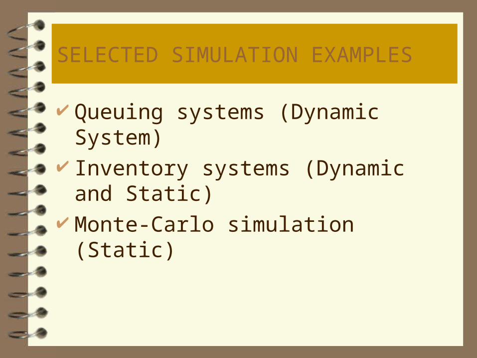
SELECTED SIMULATION EXAMPLES

Queuing systems (Dynamic System) Inventory systems (Dynamic and Static) Monte-Carlo simulation (Static)

Example: A Doctor Office

Elements of the system

Entities:– patients

Characteristics of the system

:

– Arrival process (Random Interarrivals 1-6)

– Examination or service process (Random Service Times 1-4)

– Infinite line length

– FCFS queue discipline

Elements of the system

Events:– Arrival of patients

– Completion of service (examination)

State variables:– Number of patients in the system

– Number of patients in the waiting line

– Status of doctor

Performance measures:– Time in System

– Waiting time in the line

– Utilization

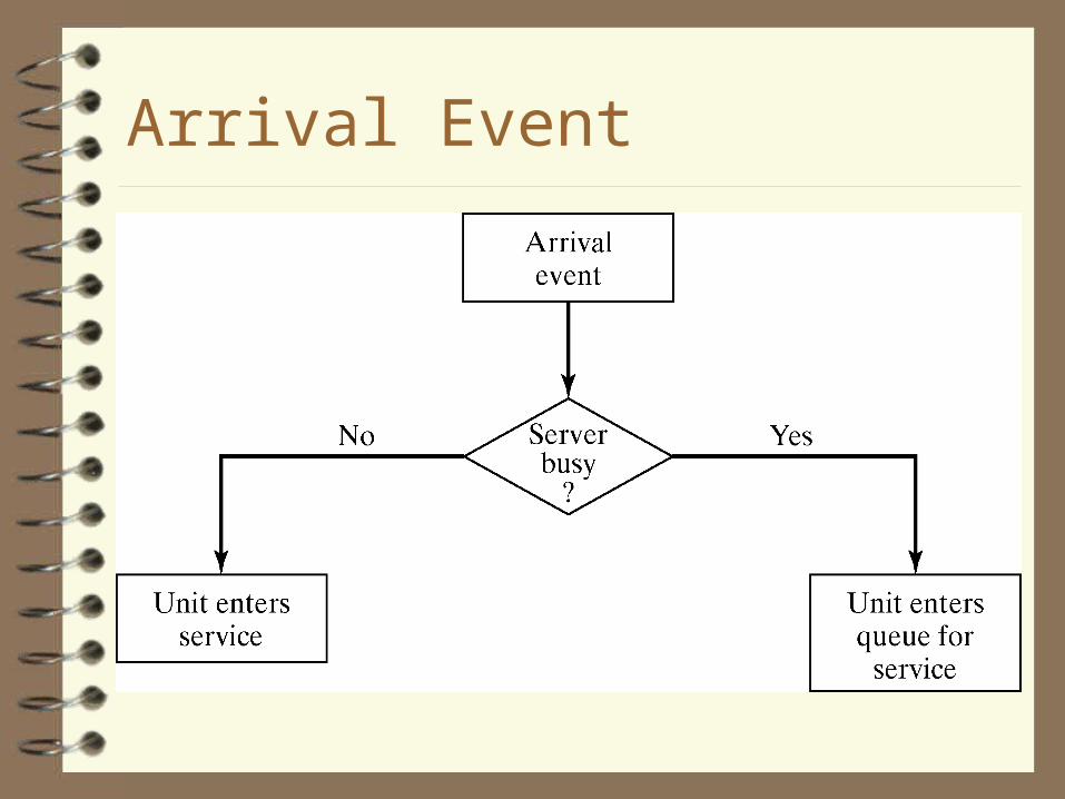
Arrival Event

Service Completion Event

Interarrival and Clock Times

Customer Interarrival Time

Arrival

Time on Clock

1 - 0

2 2 2

3 4 6

4 1 7

5 2 9

6 6 15

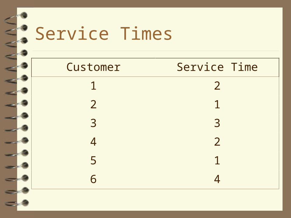
Service Times

Customer Service Time

1 2

2 1

3 3

4 2

5 1

6 4

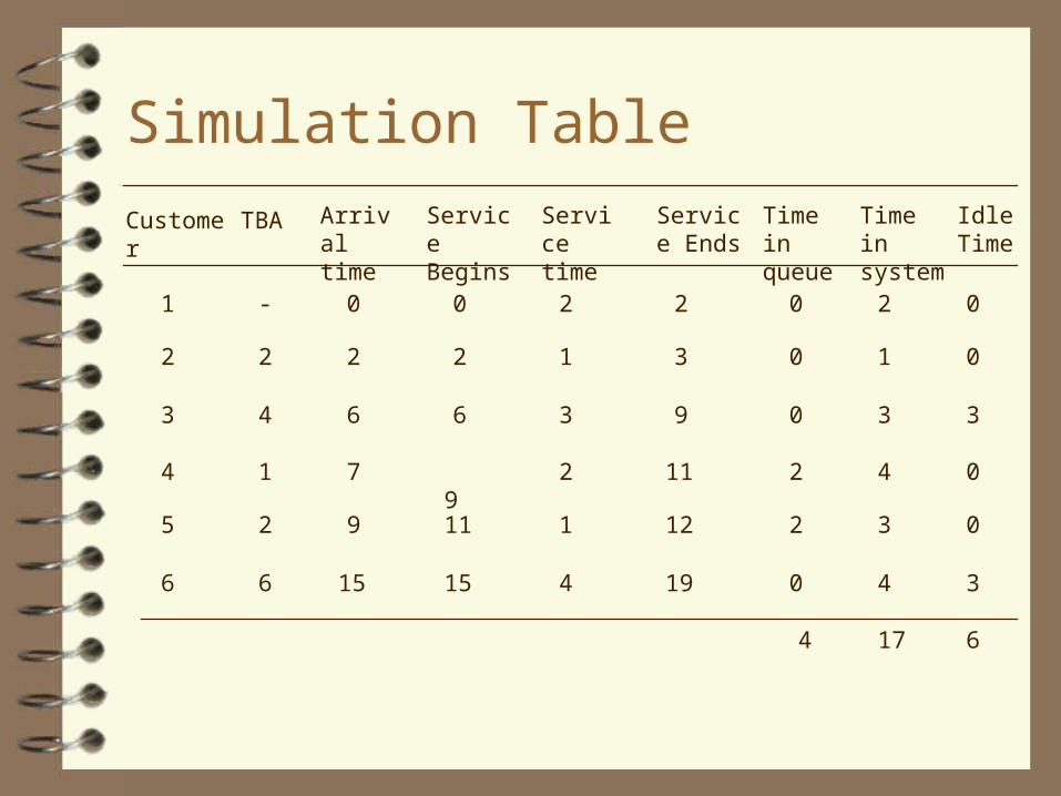
Simulation Table

1 - 0 0 2 2 0 2

2 2 2 2 1 3 0 1

3 4 6 6 3 9 0 3

Customer Arrival time

Service Begins

Service time

Service Ends

Time in queue

Time in system

Idle Time

4 17

TBA

0

0

3

4 1 7 9 2 11 2 4

5 2 9 11 1 12 2 3

6 6 15 15 4 19 0 4

0

0

3

6

Chronological Ordering of Events

Event Type Customer Number Clock Time

Arrival 1 0

Departure 1 2

Arrival 2 2

Departure 2 3

Arrival 3 6

Arrival 4 7

Departure 3 9

Arrival 5 9

Departure 4 11

Departure 5 12

Arrival 6 15

Departure 6 19

Number of Customers in the SystemN

umbe

r of

cus

tom

ers

in t

he s

yste

m

Clock Time4 8 12 16 20

2 3 5 6

4 5

4

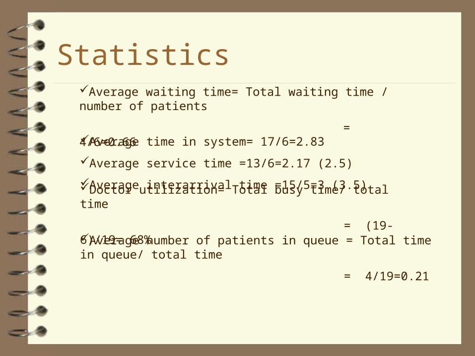
Statistics

Average waiting time= Total waiting time / number of patients

= 4/6=0.66Average time in system= 17/6=2.83

Average service time =13/6=2.17 (2.5)

Average interarrival time =15/5=3 (3.5)

Doctor utilization= Total busy time/ total time

= (19-6)/19= 68%

Average number of patients in queue = Total time in queue/ total time

= 4/19=0.21

Further questions

Can we simulate the system 10,000 patients?

How about more complex systems?

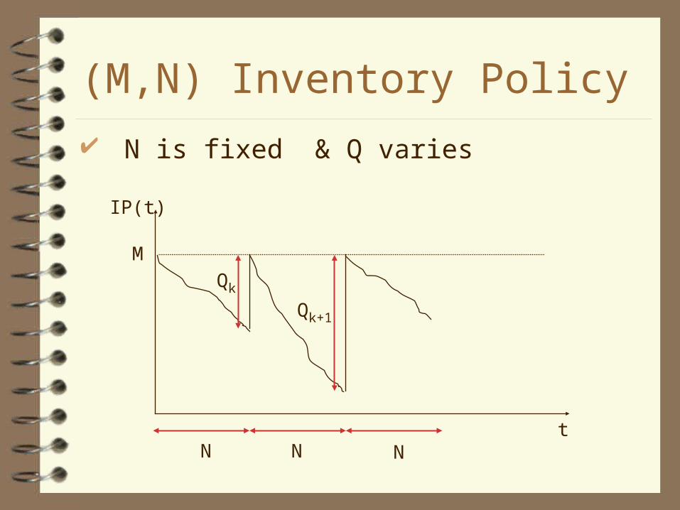
(M,N) Inventory Policy

N is fixed & Q varies

IP(t)

t

M

Qk

Qk+1

N N N

(M,N) Policy Example Review period N=5 days, Order-up-to level M=11 units (The order is given at the end of the review day and arrives at the beginning of the day after the lead-time elapses) The shortages are backordered and instantaneously satisfied the moment the replenishment order arrives Beginning inventory = 3 units; 8 units scheduled to arrive in two days Holding cost h = $1 per unit per day Shortage cost s = $2 per unit per day Ordering cost K = $10 per order

t

Question: based on 5 cycles of simulation, calculate– Average number of on-hand inventory at the end of the day– Average number of shortage per day– Average cost per day

INPUT DATA

1. Demand Distribution

Demand Probability Cumulative RD Probability Assignment 0 0.10 0.10 01-10 1 0.25 0.35 11-35 2 0.35 0.70 36-70 3 0.21 0.91 71-91 4 0.09 1.00 92-00

2. Lead Time Distribution

Lead Time Probability Cumulative RDProbability Assignment

1 0.6 0.6 1-62 0.3 0.9 7-93 0.1 1.0 0

c

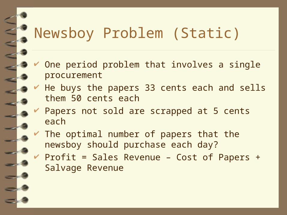
Newsboy Problem (Static)

One period problem that involves a single procurement He buys the papers 33 cents each and sells them 50 cents each Papers not sold are scrapped at 5 cents each The optimal number of papers that the newsboy should purchase

each day? Profit = Sales Revenue – Cost of Papers + Salvage Revenue

Distribution of Newspapers Demanded

Demand Probability

Cumulative

Probability

Random-Digit Assignment

40 0.03 0.03 01-03

50 0.05 0.08 04-08

60 0.15 0.23 09-23

70 0.20 0.43 24-43

80 0.35 0.78 44-78

90 0.15 0.93 79-93

100 0.07 1.00 94-00

Simulation Table

Simulation Table in Excel

MONTE-CARLO SIMULATION

Use random numbers and random sampling to approximate the outcome– stochastic and static simulation

– consists of a series random events with each event unaffected by the prior events

– (the passage of time is not a part of simulation)

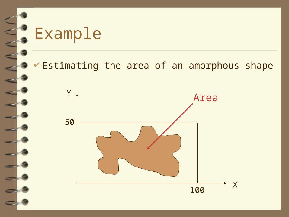
Example

Estimating the area of an amorphous shape

Y

X

50

100

Area

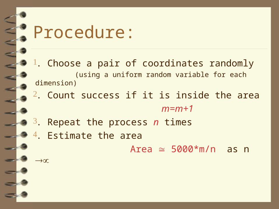
Procedure:

. Choose a pair of coordinates randomly (using a uniform random variable for each dimension)

. Count success if it is inside the area

m=m+1. Repeat the process n times. Estimate the area

Area 5000*m/n as n

Estimating the Value of

4)1Pr( 22 YX

0 1

1

X, Y ~ uniform (0,1)

Estimate value by simulation

Convergence to Point Estimates for Pi

2.90

2.95

3.00

3.05

3.10

3.15

3.20

3.25

3.30

Replications

Esti

mate

Example: Approximating integrals

One of the earliest applications

kasab

ugEk

ug

yprobabilitwiththatfollowsitnumberseloflawstrongByab

mean

withddistributeyidenticallandtindependenareugugugthen

iablesrandombaUNuniformtindependenareuuuifNow

ugEab

dxxgab

ugEbaUNuLet

dxxg

k

i

i

k

k

b

a

b

a

1

21

21

)(

,1,arg

)(...,),(),(

,var),(...,,,

1),(

Summary

Applications can be found in many areas The ad hoc methodology applied for

obtaining the simulation tables is not suitable for more complex models of dynamic systems

A more systematic methodology: event-scheduling