simulation model of the hydro-thermal power system … 1 / 18 simulation model of the hydro-thermal...
TRANSCRIPT

Page 1 / 18
Simulation Model of the Hydro-Thermal Power System in Iceland
Skuli Johannsson, Annad veldi ehf, Reykjavik, Iceland, [email protected]
Elias B Eliasson, The National Power Company, Iceland, [email protected]
14-June-2002
Introduction
Encouraged by the current trend in the European Union and the rest of the world Iceland
is on the threshold of deregulating the energy sector. The Icelandic government has
already prepared the transition from the current monopolistic system to a deregulated
system. A bill has been put forward in the Althing (the Icelandic Parliament) but it has
not yet been passed and further discussion and studies on the matter have been
postponed and are awaiting the autumn session.
The basic idea of deregulation is that instead of following an operation and expansion
plan produced by central agencies, private agents will decide on construction of
generating units and compete on an open market fore sale of power. This is supposed
to create favorable economic signals from customers and the open market to guarantee
more optimal operation and expansion than under the old system.
The small size of the Icelandic Power System and also the small population of only
270.000 has created worries if the deregulating models of the big national blocks could
be implemented in this small island in the middle of the North Atlantic. There are no
electrical connections to other countries and even though projects of submarine
transmission cables have been studied, there are vanishing probabilities that the project
will be realized in the near future.
All this is not proof that a free market can not exist in Iceland, but it is more likely here
than elsewhere, that the only possibility for both stable and beneficial solution will be
in the form of controlled oligopoly rather than unregulated competition.
The electricity sector has some characteristics that differ from other sectors and in a
considerable more complicated manner. A few such examples are:
Electricity from one producer to a customer can not be differentiated and
electricity flows through the transmission networks only according to the laws
of physics rather than commercial contractual agreements.
Electricity can not be stored economically and there has to be continuous
balance between demand and supply.
The way to store power in a hydro-thermal power system is to store excess water
in reservoir storage to be used in periods of low water supply.
There are very high requirements to reliability and costs of power shortage
accordingly high.

Page 2 / 18
There are increasing problems associated with building new hydro power plants
because of environmental considerations. In Iceland the vegetation rich dips in
the lava covered highlands are also the best places for new water reservoirs. It
is by no means guaranteed that privately owned new hydro would receive a
different attitude from the environmental movements, the political system or the
general public than under the current system.
As a consequence this sector has to be carefully monitored at all times and radical
changes in the business environment must be thoroughly prepared. Access to a good
decision support system is of paramount importance. The central part of such a system
is a simulation model to study the operational characteristics of the power system.
In this report a new simulation model of a hydro-thermal power system is presented.
The model includes all features of former models that have been used in Iceland and
also includes several new important features i.e. taking account of congestions in the
transmission system. The model is considered well suited for studies on the Icelandic
Power system in order to analyze consequences of necessary decisions when changing
the order from monopoly to deregulation.
The Icelandic Power System

Page 3 / 18
The Electrical Power System used to demonstrate the model is shown in figure 1. The
year is 2013 and the scenario includes the Karahjukar project and a new aluminium
factory in East-Iceland, both fully operational.
The system is divided into 3 subsystems: South-West, North and East. Transmission
capacity between subsystems is not sufficient for free interchange of power.
The main characteristics of this power system are shown in table 1.
Table 1 Main characteristics of the Icelandic power system 2013
Item Unit Total S-West North East
Energy inflow to reservoirs GWh/y 9,020 2,565 875 5,580
Energy in other inflow GWh/y 6,475 5,285 1,030 160
Total inflow of energy GWh/y 15,495 7,850 1,905 5,740
Energy demand GWh/y 14,975 7,925 840 6,210
Energy balance GWh/y 520 -75 1,065 -470
Reservoir storage capacity GWh 4,395 1,395 285 2,715
Storage in % of demand % 29% 18% 34% 44%
Hydro plants MW 1,760 876 193 691
Geothermal plants MW 237 151 86 0
Total Hydro and Geothermal MW 1,997 1,027 279 691
Interruptible power, class A a) MW 162 63 21 78
Interruptible power, class B MW 49 49 0 0
Thermal reserve power MW 104 47 41 16
Interruptible power, class C MW 91 39 0 52 a) time dependent series
The three big reservoirs are glacier fed so inflow is highly correlated with yearly
temperature distribution.
The limited storage capacity in the South-West is compensated by a substantial
groundwater flow from the porous lava covered highlands throughout the winter.
The geothermal plants get steam from over 2000 meters deep boreholes and are
unaffected by weather conditions. Thus synergy is created between those power
resources by relatively diminishing the extent of shortage in extreme low water years
while preserving the flexibility of the hydro.
The transmission system is modelled as a three-node network and 132 kV transmission
lines between subsystems are defined by the figures in the parenthesis:
(Capacity in GWh/week; Energy losses in %).
(13.45; 5%) North (14.83; 6%)
South-West East
(11.55; 5%)

Page 4 / 18
Hydrothermal Scheduling
Hydrothermal Scheduling models aim at optimal use of hydro and geothermal
resources, in relation to the characteristics of the generation capacity, uncertain future
inflows, thermal generation, power demand and costs of transmission between
subsystems.
The most important aspect of the Icelandic Power System is the utilization of water
stored in reservoirs under the constraints of isolation from other systems and limited
backup capacity in the form of fossil plants.
Traditional water value methods involve using a strategic part to create an optimal
operations policy for the hydro-thermal power system in Iceland. There after
simulations are performed for the purpose of mapping the characteristics of the system,
creating probabilistic views into the future for the purpose of operation planning,
expansion planning and optimization of hydro plants and their components.
The current method is based on the concept of a monopolistic system and only one
overall water value is calculated for the whole country. Some important factors are
obscured by this simplification, like:
different hydrological conditions in different parts of the country
geographical distribution of the power demand and production
power exchanges
effects of transmission losses and congestions.
The model presented here is meant to take all this into account , thus in effect creating
coherent operation policies although independent for each part of the country. The
model has features to make studies possible in an open market condition. Its main
features are:
The system can be divided into subsystems of any number and connected by
power lines in any configuration.
Transmission constraints and losses between subsystems can be defined.
Water values are calculated for each subsystem taking into account local market,
local production and energy transmission in and out of the subsystem.
Time unit in the model is one week and calculations are based on river flow series for
the years 1950-2000, totaling 51 years.
Page 5 / 18
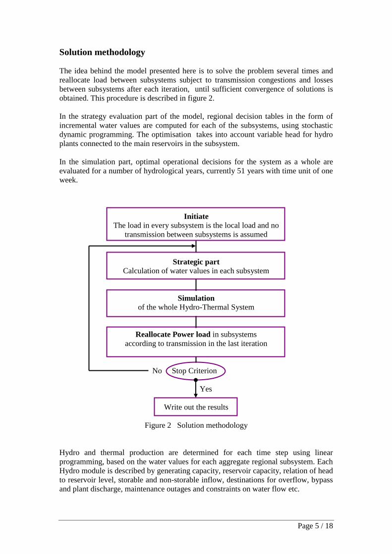
Solution methodology
The idea behind the model presented here is to solve the problem several times and
reallocate load between subsystems subject to transmission congestions and losses
between subsystems after each iteration, until sufficient convergence of solutions is
obtained. This procedure is described in figure 2.
In the strategy evaluation part of the model, regional decision tables in the form of
incremental water values are computed for each of the subsystems, using stochastic
dynamic programming. The optimisation takes into account variable head for hydro
plants connected to the main reservoirs in the subsystem.
In the simulation part, optimal operational decisions for the system as a whole are
evaluated for a number of hydrological years, currently 51 years with time unit of one
week.
Initiate
The load in every subsystem is the local load and no
transmission between subsystems is assumed
Strategic part
Calculation of water values in each subsystem
Simulation
of the whole Hydro-Thermal System
Reallocate Power load in subsystems
according to transmission in the last iteration
No Stop Criterion
Yes
Write out the results
Figure 2 Solution methodology
Hydro and thermal production are determined for each time step using linear
programming, based on the water values for each aggregate regional subsystem. Each
Hydro module is described by generating capacity, reservoir capacity, relation of head
to reservoir level, storable and non-storable inflow, destinations for overflow, bypass
and plant discharge, maintenance outages and constraints on water flow etc.

Page 6 / 18
The new model will after completion be used for studying the operation of the Power
System and for expansion studies both for generation and transmission capacity
alternatives.
Some of the categories of intended studies are as follows:
Market
Spot price forecasting in deregulated markets
Risk assessment in dry water years
Price evaluation for financial contracts with large industries
Generating system
Long-term operational scheduling of hydropower
Reservoir operation
Analysis of overflow losses
Calculation of probability of power production in the hydro-, geothermal and
thermal power plants in each subsystem
Maintenance planning
Expansion planning of generating capacity
Probability distribution of operational costs within each area
Transmission System
Utilization of transmission capacity between subsystems – duration curves.
Expansion planning of transmission capacity between subsystems.
Calculation of Water Values
With reservoirs it is possible to store excess water in the summertime when demand is
minimal to be used in the wintertime when demand is high.
In the strategic part of the problem as described in figure 2 the value of water in
reservoirs is calculated.
Water value is an evaluation of operational cost for the power system in the future that
can be avoided by storing water in reservoirs for later use instead of using it
immediately.
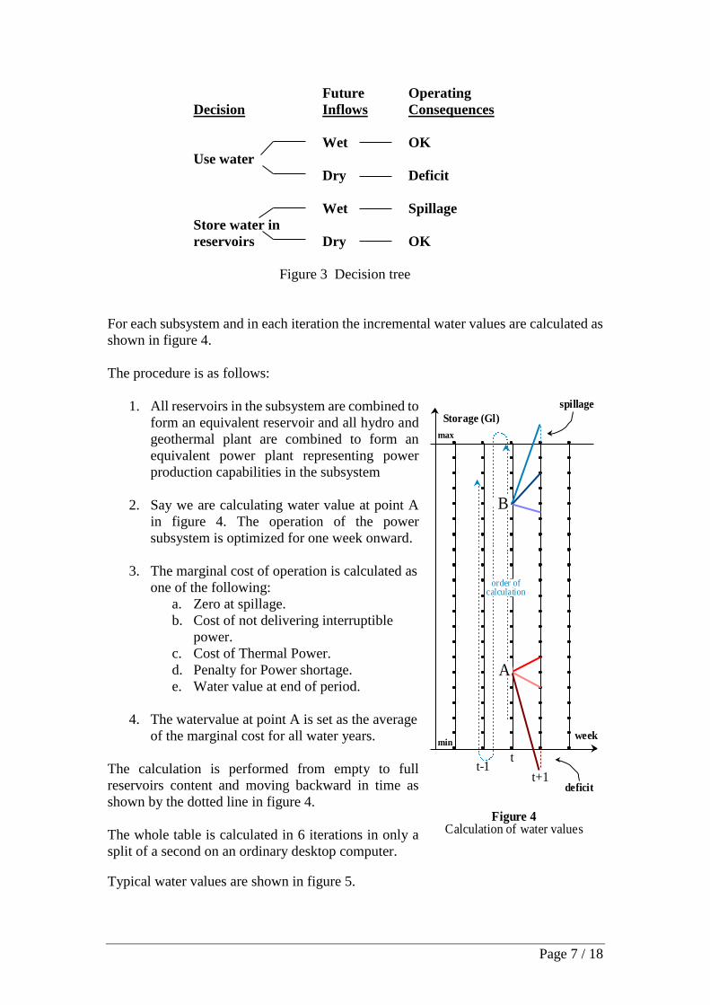
The decision process can be explained in a decision tree:
Page 7 / 18
Future Operating
Decision Inflows Consequences
Wet OK
Use water
Dry Deficit
Wet Spillage
Store water in
reservoirs Dry OK
Figure 3 Decision tree
For each subsystem and in each iteration the incremental water values are calculated as
shown in figure 4.
The procedure is as follows:
1. All reservoirs in the subsystem are combined to
form an equivalent reservoir and all hydro and
geothermal plant are combined to form an
equivalent power plant representing power
production capabilities in the subsystem
2. Say we are calculating water value at point A
in figure 4. The operation of the power
subsystem is optimized for one week onward.
3. The marginal cost of operation is calculated as
one of the following:
a. Zero at spillage.
b. Cost of not delivering interruptible
power.
c. Cost of Thermal Power.
d. Penalty for Power shortage.
e. Water value at end of period.
4. The watervalue at point A is set as the average
of the marginal cost for all water years.
The calculation is performed from empty to full
reservoirs content and moving backward in time as
shown by the dotted line in figure 4.
The whole table is calculated in 6 iterations in only a
split of a second on an ordinary desktop computer.
Typical water values are shown in figure 5.
Figure 4Calculation of water values
max
week
Storage (Gl)
spillage
t
t+1t-1
deficit
min
order ofcalculation
A
B

Page 8 / 18
Formulation of the Hydrothermal Dispatch
Objective Function
Given the water values for reservoirs in each subsystem the objective is to minimize
the sum of immediate and future operating costs:
min c(j) gt(j) + (k,vt+1) t+1(k) vt+1(k) (1)
c(j)gt(j) the immediate cost is given by the thermal operating costs in stage t
(k,vt+1) t+1(k) vt+1(k) the future cost is represented by:
(k,vt+1) production coefficient of reservoir k (GWh/Gl);
can vary with reservoir content.
t+1(k) the water value function of reservoir content in
(Mkr/Gwh=kr/kWh)
vt+1(k) reservoir volume at the end of stage t (start of stage t+1)
in (Gl).
The operating constraints are as follows:
Load Supply
For each subsystem:
(i,vt+1) ut(i) +gt(j) - (1+) L++ L- = dt (2)
where:
(i,vt+1) ut(i) Hydro production in the subsystem
gt(j) Thermal production in the subsystem
(1+) L+ Sum of all power exports from the subsystem incl losses
L- Sum of all power imports to the subsystem
The transmission L in each power line between subsystems is represented by two
components one in each direction:
L = L+ + L- (3)
Water balance.
The water balance equation relates storage and outflow. Reservoir storage at the end of
stage t (beginning of stage t+1) is equal to initial storage minus outflow volumes
(turbined and spilled) plus inflow volumes (lateral inflow plus releases from upstream
plants):
Page 9 / 18
vt+1(i) = vt(i) - ut(i) - st(i) + at(i) + [ut(m) + st(m)] (4)
mU(i)
where:
i index for hydro plants
vt+1(i) stored volume in plant i at the end of stage t
vt(i) stored volume in plant i at the beginning of stage t
at(i) lateral stream flow arriving at plant i in stage t
ut(i) turbined outflow during stage t
st(i) spilled outflow volume in plant i during stage t
mU(i) set of plants immediately upstream of plant i
Limits on Storage and Outflow
vt(i) v(i)
(5)
ut(i) u(i)
where v(i) and u(i) are respectively the maximum storage and turbine capacities.
Limits on Thermal Generation
gt(j) g (j) (6)
The objective function with the operational constraints represent a standard linear
programming optimisation problem that can be easily solved with software packages
that are commercially available.
The signature in the formulation of the problem is taken from [1].
Case study
A case study was performed based on a scenario of the Icelandic Power system in the
year 2013 as shown in figure 1.
The overall demand in this case is actually very high compared to the power production
capability of the system. As seen in table 1 there is an excessive production capability
in the North but an insufficient production capability in the South-West and the East.
The model balances this incompatibility by simulating transmission of power between
the subsystems.
The simulation uses river flow series for the water years 1950-2000 (51 years) and the
model is based on the methodology shown in figure 2. Time unit is one week.

Page 10 / 18
It is worth observing that one simulation, which reallocates load 5 times to iterate to a
stable solution according to figure 2, takes about 70 seconds on a small desktop IBM
computer NetVista with a 733 Mhz Pentium 3 processor and 384 Mb RAM. This
includes reading in data of river flow and demand, calculating water values 90 times,
solving 13.260 linear optimisations (40 rows and 60 columns) and writing out extensive
files than can be imported easily to EXCEL.
The program is written in C++ and uses a DLL linear programming package from
Frontline Systems Inc in USA.
In the simulation, volume of the reservoir at the end of one water year was used as the
volume in the beginning of the following water year.
The system was divided into three subsystems according to figure 1. Main
characteristics of the power system used in the simulation are described in table 1.
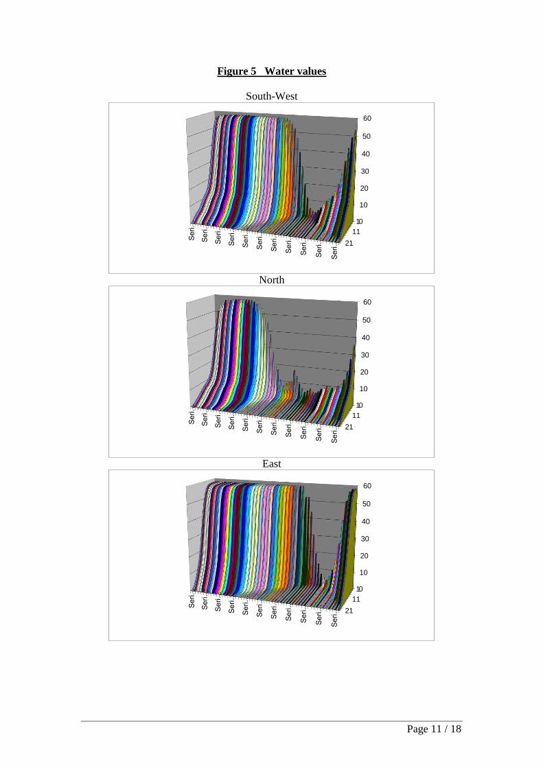
Figure 5 shows the resulting water values of each subsystem after the 5 iterations.
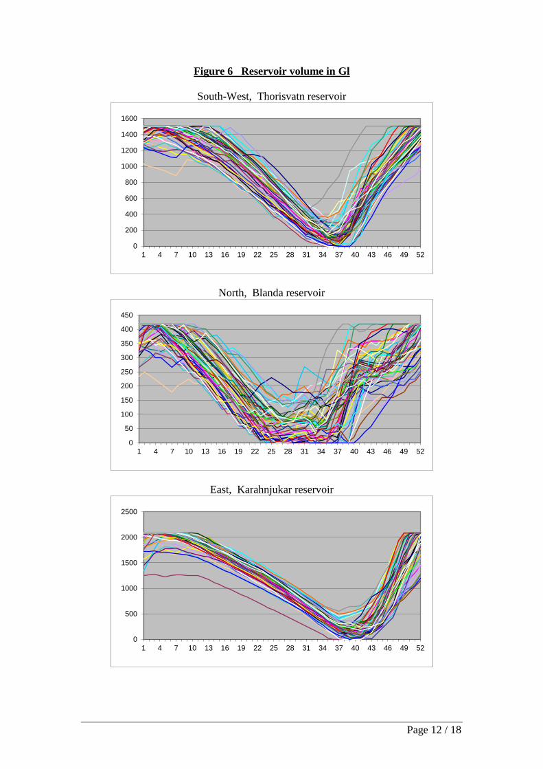
Figure 6 shows the volume of the three reservoirs in the subsystems as a group of
curves, one curve for each of the 51 water years used in the simulation model. The
group of curves reflects visually the expected mean and variation and also the extreme
values of reservoir content within the year.
Figure 7 shows the resulting shadow prices for energy market in each subsystem, also
as a group of curves.
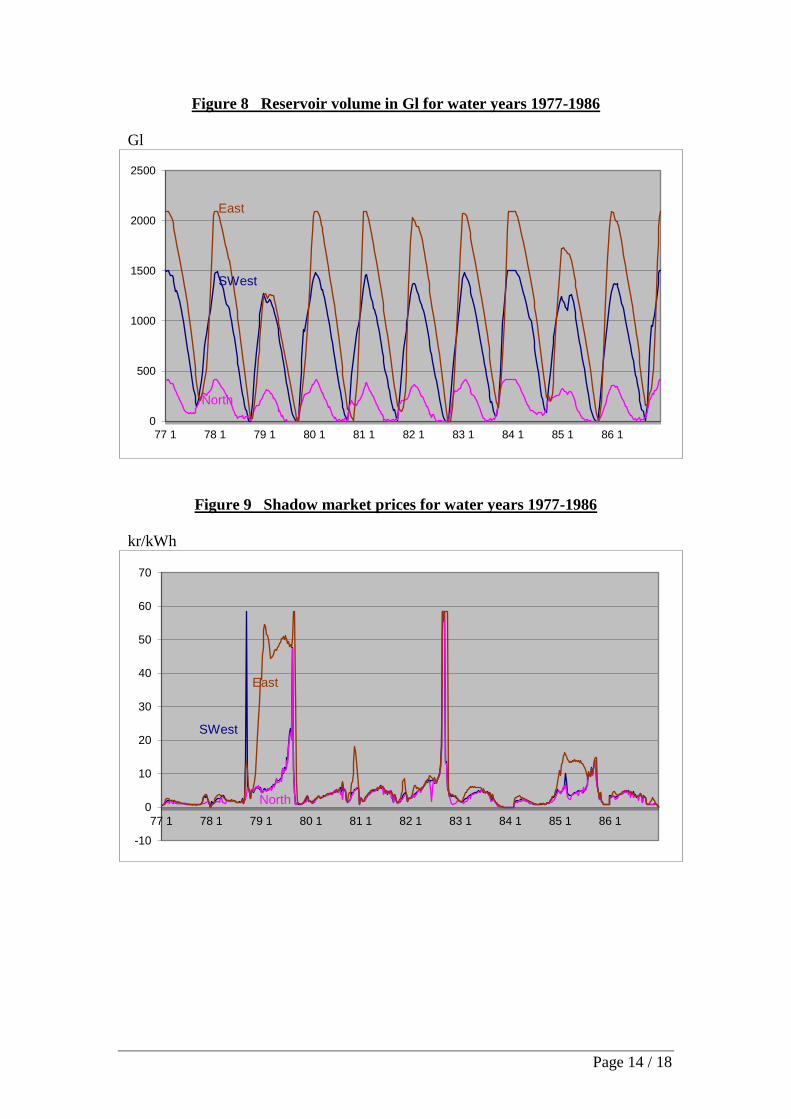
Figure 8 shows in more detail 10 years (1977-1986) of the 51 water years used in the
simulation. As shown the drawdown of the reservoir in the East is 4-5 weeks later than
in the South-West reflecting that spring arrives that much later. This explains one of
the most important feature of the model i.e. how it takes account of different
hydrological conditions in the subsystems and the operation is optimised according to
that.
Figure 9 shows for the same years the evaluation of the market shadow prices. The
heavier demand compared to production capability in the East results in higher shadow
prices caused by bottlenecks in the transmission system. Most of the time the three
subsystems have the same shadow price reflecting that during that time congestions in
the transmission network do not limit exchange of power as needed for cost
minimization.
Simulation results have shown that if transmission constraints are eliminated by
doubling or tripling the transmission capabilities between the subsystems the shadow
prices will be the same in all the subsystems. The resulting values are actually the
trajectory of water values throughout the simulation, and those water values are actually
the marginal cost of the system at every time.
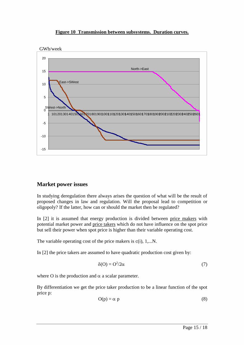
Figure 10 shows transmission in the high voltage power lines between subsystems as
duration curves. This is very important piece of information regarding feasibility
studies in expansion planning of the overall transmission network.
Page 11 / 18
Figure 5 Water values
South-West
North
East
Seri…
Seri…
Seri…
Seri…
Seri…
Seri…
Seri…
Seri…
Seri…
Seri…
Seri…
0
10
20
30
40
50
60
1
11
21
Seri…
Seri…
Seri…
Seri…
Seri…
Seri…
Seri…
Seri…
Seri…
Seri…
Seri…
0
10
20
30
40
50
60
1
11
21
Seri…
Seri…
Seri…
Seri…
Seri…
Seri…
Seri…
Seri…
Seri…
Seri…
Seri…
0
10
20
30
40
50
60
1
11
21
Page 12 / 18
Figure 6 Reservoir volume in Gl
South-West, Thorisvatn reservoir
North, Blanda reservoir
East, Karahnjukar reservoir
0
200
400
600
800
1000
1200
1400
1600
1 4 7 10 13 16 19 22 25 28 31 34 37 40 43 46 49 52
0
50
100
150
200
250
300
350
400
450
1 4 7 10 13 16 19 22 25 28 31 34 37 40 43 46 49 52
0
500
1000
1500
2000
2500
1 4 7 10 13 16 19 22 25 28 31 34 37 40 43 46 49 52

Page 13 / 18
Figure 7 Shadow prices in kr/kwh or Mkr/GWh
South-West
North
East
-10
0
10
20
30
40
50
60
70
1 4 7 10 13 16 19 22 25 28 31 34 37 40 43 46 49 52
-10
0
10
20
30
40
50
60
70
1 4 7 10 13 16 19 22 25 28 31 34 37 40 43 46 49 52
-10
0
10
20
30
40
50
60
70
1 4 7 10 13 16 19 22 25 28 31 34 37 40 43 46 49 52
Page 14 / 18
Figure 8 Reservoir volume in Gl for water years 1977-1986
Gl
Figure 9 Shadow market prices for water years 1977-1986
kr/kWh
0
500
1000
1500
2000
2500
77 1 78 1 79 1 80 1 81 1 82 1 83 1 84 1 85 1 86 1
East
SWest
North
-10
0
10
20
30
40
50
60
70
77 1 78 1 79 1 80 1 81 1 82 1 83 1 84 1 85 1 86 1
East
North
SWest
Page 15 / 18
Figure 10 Transmission between subsystems. Duration curves.
GWh/week
Market power issues
In studying deregulation there always arises the question of what will be the result of
proposed changes in law and regulation. Will the proposal lead to competition or
oligopoly? If the latter, how can or should the market then be regulated?
In [2] it is assumed that energy production is divided between price makers with
potential market power and price takers which do not have influence on the spot price
but sell their power when spot price is higher than their variable operating cost.
The variable operating cost of the price makers is c(i), 1,...N.
In [2] the price takers are assumed to have quadratic production cost given by:
(O) = O2/2 (7)
where O is the production and a scalar parameter.
By differentiation we get the price taker production to be a linear function of the spot
price p:
O(p) = p (8)
-15
-10
-5
0
5
10
15
20
1 10120130140150160170180190110011101120113011401150116011701180119012001210122012301240125012601
North->East
SWest->North
East->SWest
Page 16 / 18
The spot price can be related to the total price makers production Q:
p(Q) = (D-Q)/ (9)
where D is the total demand.
By using the Nash-Cournot equilibrium in [2] the total price makers energy production
is given by:
ND - c(i)
Q = (10)
N+1
Lets assume there are three main players (N = 3) on the Icelandic power market, one in
each subsystem, and their variable cost of production c(i) is defined by the market
shadow prices that have now been calculated by the simulation model.
One way to identify the price takers is to arrange all classes of interruptible power,
thermal plants and penalty cost for shortage in increasing order by price and capacity
and approximate it with a quadratic cost function . The result for whole of Iceland is a
rough estimate of 40.
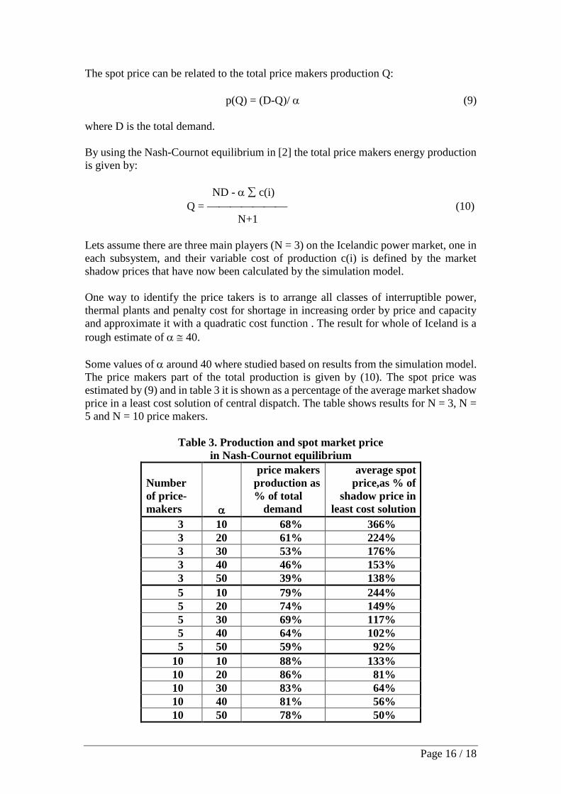
Some values of around 40 where studied based on results from the simulation model.
The price makers part of the total production is given by (10). The spot price was
estimated by (9) and in table 3 it is shown as a percentage of the average market shadow
price in a least cost solution of central dispatch. The table shows results for N = 3, N =
5 and N = 10 price makers.
Table 3. Production and spot market price
in Nash-Cournot equilibrium
Number
of price-
makers
price makers
production as
% of total
demand
average spot
price,as % of
shadow price in
least cost solution
3 10 68% 366%
3 20 61% 224%
3 30 53% 176%
3 40 46% 153%
3 50 39% 138%
5 10 79% 244%
5 20 74% 149%
5 30 69% 117%
5 40 64% 102%
5 50 59% 92%
10 10 88% 133%
10 20 86% 81%
10 30 83% 64%
10 40 81% 56%
10 50 78% 50%

Page 17 / 18
We notice from table 3 that for N = 3 and =40 we get the average spot price as 1,53
times the average shadow price. At the same time the production level of the price
makers is down to only 46% of the total demand which is inconceivable in the Icelandic
market.
Table 3 shows that only three price makers competing in the market are too few to
establish a real competition. The spot market tends to be all too high. The rule of thumb
is that to create some kind of genuine competition there must be at least 5 equally sized
price makers acting on the market which is more than the foreseeable number.
The National Power Company could eventually sell some of its power plants to
investors or the aluminium industries could be allowed to become active players on
the market by decreasing their production level in times of increasing demand and spot
market price. Thereby enabling them to sell their buying rights to other agents in the
market. Neither arrangement has yet been considered nor a plausible method to find the
market value of each plant has been realized.
In Iceland long-term contracts with the heavy industries at a fixed price already make
up a large proportion of energy transactions. If the heavy industries are allowed to sell
parts of their power contracts on the market can this be regulated so that the resulting
price distortions do not become intolerable to other players?
The Nash-Cournot competition model is based on the assumption that agents on the
market will compete in quantities which is also the probable outcome after deregulation
in Iceland. It can be argued that the large water reservoirs feeding downstream hydro
plants play a significant role in that respect. The owners of the reservoirs have the
possibility to regulate water use from the reservoirs in a different way than would be
practiced by a central dispatch aiming at overall cost minimization. In that way situation
of water shortage and therefore rise in energy prices could be easily manipulated by the
reservoir owners. They also have the market power to offer very cheap energy on the
market in times of water spillage to play the competition out of the market.
The only substantial owner of water reservoirs in Iceland today is the National Power
Company, Landsvirkjun, and then they have the potential of becoming the sole price
maker in the country. The question arises, what the terms are under which this can be
allowed and still having some form of a competition on the power market.

Page 18 / 18
References.
[1] Mario Pereira, Nora Campodonico, Rafael Kelman: “Longterm Hydro
Scheduling based on Stochastic Models” Power Systems Research Inc,
PSRI Rio de Janeiro, Brazil.
[2] Rafael Kelman, Luiz Augosto N. Barroso, Mario Veiga Pereira: “Market
Power Assessment and Mitigation in Hydrothermal Systems”.
[3] Skuli Johannsson, Annad veldi ehf, Reykjavik: “Nytt hermilikan fyrir
raforkukerfi Landsvirkjunar”. Prepared for the National Power Company in
Iceland, March 2002. (In Icelandic).
[4] Skuli Johannsson, Annad veldi ehf, Reykjavik and Elias B Eliasson, the
National Power Company: “Fakeppni a frjalsum raforkumarkadi”. Prepared
for the National Power Company in Iceland, April 2002. (In Icelandic).