simulation of beamforming by massive mimo antennas...
TRANSCRIPT

Simulation of Beamforming by Massive MIMO Antennas in Dense
Urban EnvironmentsAuthors: Greg Skidmore, Dr. Gary Bedrosian
Speaker: Greg Skidmore, Remcom, Inc.
Sep 20, 2016
Introduction
• This paper presents innovative and optimized approach to channel modeling for massive MIMO, a key technology for 5G
• Our approach:– Extends 3D ray-tracing, and addresses shortfalls identified in literature– Significant optimizations allow simulations between each Transmit and
Receive antenna in reasonable time (this is critical!)
• Study: uses to simulate beamforming with MRT and ZFBF– Calculate power, SINR, and interference– Predict impact of pilot contamination
Overall: provides new insight into the nature of beams in urban settings and demonstrates value of new MIMO simulation capability
2

Objectives of 5G
3
Key Objectives Move Toward Connected Information Society [1]
Massive Growth in Mobile Data Demand
Massive Growth in Connected Devices
Increasingly Diverse Use Cases &
Requirements
10-100x Data Rates (~10 Gbps)
1000x Capacity
10-100x Devices (50-500B)
5x Lower Latency
100x Energy Efficiency
10x Longer Battery Life for Low-power Devices
Challenges Objectives
Potential Benefits of Massive MIMO[1]-[3]
• Increases capacity 10x via spatial multiplexing
• Improves radiated energy-efficiency 100x
– Directs signal to user, reducing power & interference
• Can use inexpensive, low-power components
• Reduces latency, eliminates fading
• More robust to interference and jamming
4
Channel Modeling for 5G
• Organizations such as 3GPP and METIS have researched channel modeling requirements; METIS* requirements for 5G include [4]:– Very high bandwidths (hundreds of MHz)– Full three-dimensional & accurate polarization modeling– Massive MIMO: spherical waves and high spatial resolution– Extremely large array antennas– Spatial consistency as points move or are in close proximity– Wide range of propagation scenarios– Wide frequency range (<1GHz up to 86+ GHz)– Dual-mobility for D2D, M2M, V2V– Importance of diffuse vs. specular scattering at mm wave
5
Our approach focuses on these MIMO-relevant requirements* Mobile and wireless communications Enablers for Twenty-
twenty (2020) Information Society

Simulating MIMO with 3D Ray-Tracing
• Use Wireless InSite® to simulate MIMO channels
• 3D ray-tracing provides data required by MIMO algorithms– Complex path gain– Full resolution of spherical &
diffracted waves across array– 3D path data w/full time, angle
& polarization information– Complete spatial consistency
throughout complex scenes
• But: out-of-box, very complex for traditional ray-tracers
6
Propagation Paths for Channel between 1 Transmit/Receive MIMO Antenna Pair

New Wireless InSite® MIMO Capability
• New capability offers innovative optimizations that made several parts of study possible– Starting Point: GPU-accelerated / multithreaded X3D ray model
in Wireless InSite as starting point– Optimizations: Two key optimizations allow calculations within
timeframes on same order as single-antenna simulations:• Adjacent Path Generation (APG): leverages path data for coarse points• MIMO exact path correction: finds precise paths to array elements
– Result: precise path data between each Tx-Rx MIMO antenna pair while minimizing additional ray-tracing calculations
• These optimizations were critical for simulating a 128-element MIMO array
7
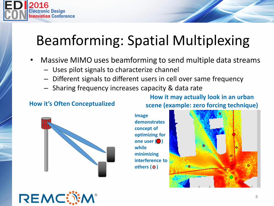
Beamforming: Spatial Multiplexing• Massive MIMO uses beamforming to send multiple data streams
– Uses pilot signals to characterize channel– Different signals to different users in cell over same frequency– Sharing frequency increases capacity & data rate
8
How it’s Often ConceptualizedHow it may actually look in an urban
scene (example: zero forcing technique)
Image demonstrates concept of optimizing for one user ( ) while minimizing interference to others ( )

Beamforming Techniques in this Study
• Investigated two techniques: 1) Max. Ratio Transmission (MRT)
Sets beamforming weights for device to maximize sum of channel gains
2) Zero Forcing (ZF)Sets beamforming weights to minimize interference to all other users in cell, placing them within local nulls
• Post-processed Results – Developed tools to extract
simulation results and calculate beamforming weights
– Used Matlab scripts provided by authors of [5] to calculate MRT and ZF weighting vectors
9
Intended device(otherdevices)
Maximum Ratio Transmission
Intended device(otherdevices)
Zero Forcing

10
MIMO Simulation Scenario:Urban Small Cell in Rosslyn, Virginia
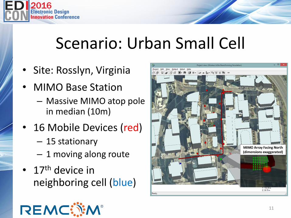
Scenario: Urban Small Cell
• Site: Rosslyn, Virginia
• MIMO Base Station– Massive MIMO atop pole
in median (10m)
• 16 Mobile Devices (red)– 15 stationary
– 1 moving along route
• 17th device in neighboring cell (blue)
11

Massive MIMO Antenna
• Frequency: 28 GHz
• 128 antennas
– 8x8 w/cross-pol
– Dipoles (for simplicity)
• Dimensions
– ½-λ spacing (1.07cm)
– 4.3cm x 4.3cm
12

Field Map for a Single Element
• Field map shows significant multipath– Strongest in LOS North &
West of base station
– Multipath extends into street to Northwest
13
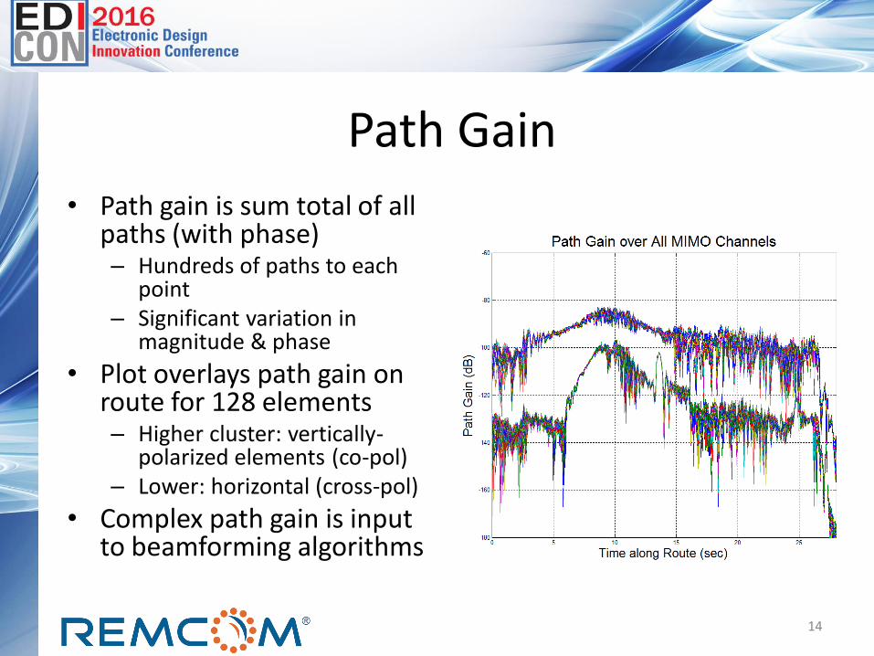
Path Gain
• Path gain is sum total of all paths (with phase)– Hundreds of paths to each
point– Significant variation in
magnitude & phase
• Plot overlays path gain on route for 128 elements– Higher cluster: vertically-
polarized elements (co-pol)– Lower: horizontal (cross-pol)
• Complex path gain is input to beamforming algorithms
14

Comparing Beamforming TechniquesMRT: maximizes beam to device, ignoring interference to others
Zero-Forcing: minimizes interference to other devices (clear difference)
15

Comparing Beamforming TechniquesMRT: maximizes beam to device, ignoring interference to others
Zero-Forcing: minimizes interference to other devices (clear difference)
16

Movies: MIMO Beamforming in MotionMaximum Ratio Transmission
(MRT) Beamforming Zero Forcing (ZF) Beamforming
17
Click to watch the movie. Click to watch the movie.

Signal-to-Interference+Noise (SINR)
• SINR is a key measure for determining capacity of a channel
• Interference is the total power of signals received by a device that are part of beams directed to other devices
18
Dev 1Dev 2
Signal
Interference + NoiseSINR =

Signal-to-Interference+Noise
• Calculated SINR– Power: assumed 10W
over Tx array
– Interference: summed power of beams to all other devices
– Noise: -87dBm, using [6]
• ZF much better than MRT for this scenario– 15-40dB higher over
most of route
19
Comparing SINR for MRT and ZF Beamforming Techniques

Details on Power, Interference & SINR
• MRT delivers more power, but ZF suppresses interference, providing much higher SINR
20
Mean Over Route MRT ZFReceived Power (dBm) -49.0 -63.0Interference (dBm) -47.9 Negl.*SINR (dB) -3.7 21.6
Table 2: Received Power and SINR for moving Device
*Interference for ZF was negligible (well below noise floor)
MRT: 14dB higher power
ZF: 25dB higher SINR

Pilot Contamination
• MIMO system uses pilot sequences to estimate channels– Because possible orthogonal sequences limited by channel coherence
time, adjacent cells likely to overlap
• Same pilot from multiple terminals degrades channel estimate– May reduce SINR to user in cell– May direct more interference toward user in adjacent cell
21
Base Station 1
Base Station 2
Pilot sequence to Local Base StationPilot Contamination (nearby B.S.)

Pilot Contamination Scenario
Device in nearby cell shares pilot signal with moving device (pilot contamination)
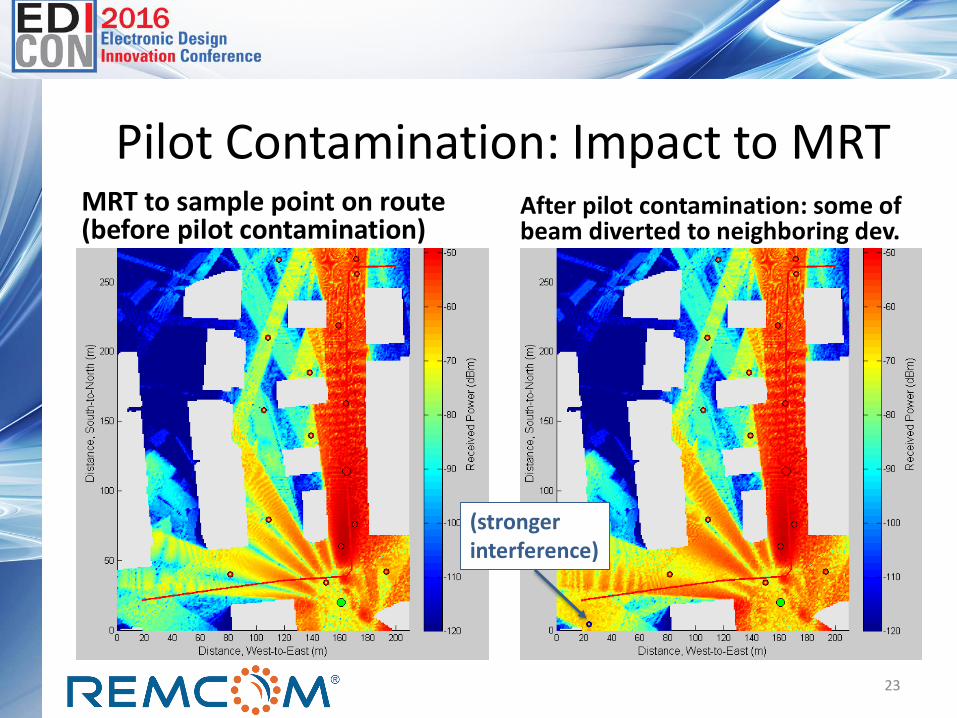
Pilot Contamination: Impact to MRTMRT to sample point on route (before pilot contamination)
After pilot contamination: some of beam diverted to neighboring dev.
23
(strongerinterference)
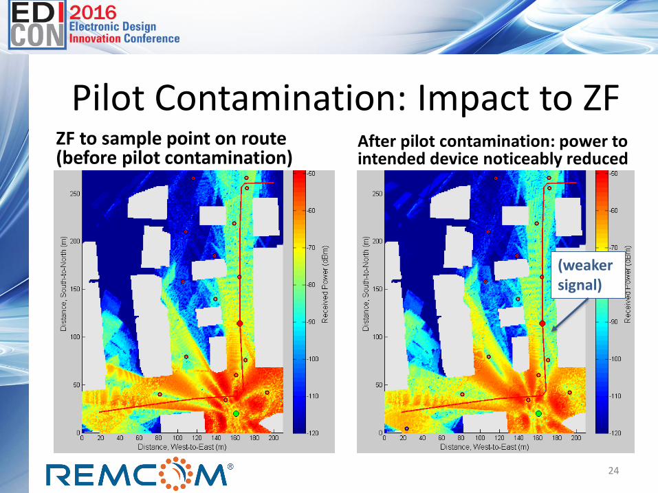
Pilot Contamination: Impact to ZFZF to sample point on route (before pilot contamination)
After pilot contamination: power to intended device noticeably reduced
24
(weaker signal)
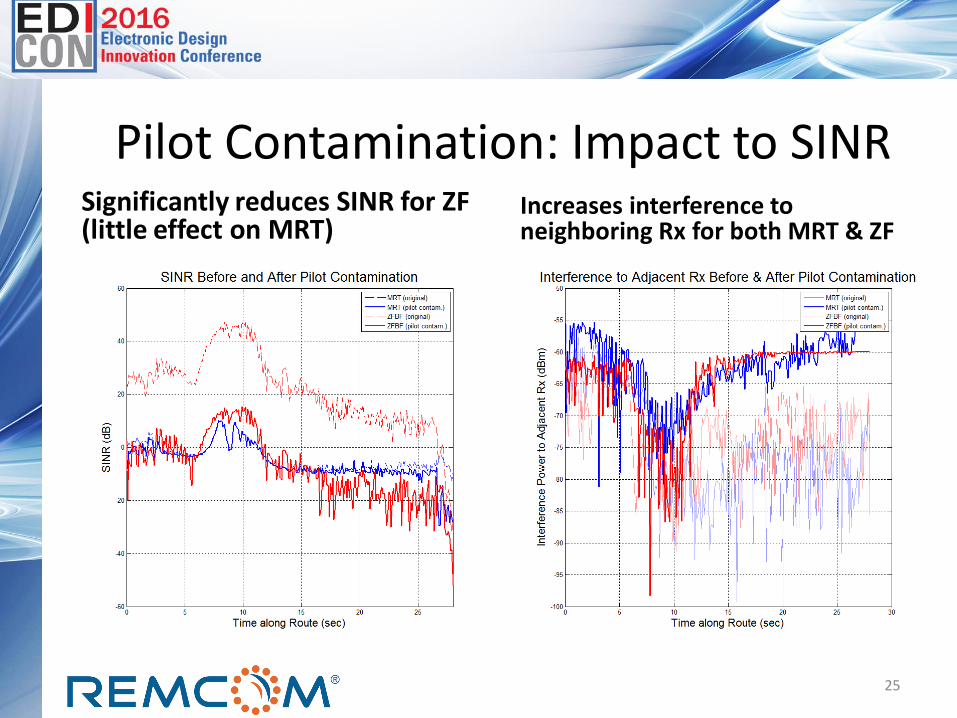
Pilot Contamination: Impact to SINRSignificantly reduces SINR for ZF (little effect on MRT)
Increases interference to neighboring Rx for both MRT & ZF
25

Pilot Contamination: Impact to SINR
26
Table 1: Effect on Local Cell
*Interference for ZF increases from well below noise floor
to above signal, significantly reducing SINR.
Beam Mean Values Over Route
Orig. PilotCont
Change
MRT Interference (dBm) -75.1 -62.6 +12.4
ZF Interference (dBm) -73.3 -64.5 +8.8
Beam Mean Values Over Route
Orig. PilotCont
Change
MRT Rcvd. Pwr. (dBm) -49.0 -51.0 -1.9Interference (dBm) -47.9 -47.9 0SINR (dB) -3.7 -5.6 -1.9
ZF Rcvd. Pwr. (dBm) -63.0 -68.6 -5.6Interference (dBm) Neg.* -64.2 High*SINR (dB) 21.6 -7.6 -29.1
Table 2: Interference to Neighboring Device
MRT: minor impact to SINR
ZF: small reduction in power; big increase to interferenceResult: SINR 29dB lower!
Both techniques increase interference (9-12dB)

Value of Simulation Optimizations• Recorded run times for sims in
this study
– High-end PC: Intel i7-3770, 32GB RAM, Quadro K620 GPU
– Recorded sim times for 3 cases
• Estimated baseline without optimizations (1 sim/antenna)
• Result: 51X – 94X faster than traditional (brute-force) approach
• Makes sims like beamforming field map possible
Simulation Case MobileDevices317 pts
FieldMap66K pts
Single Antenna (SISO) Before optimizations APG accelerated
36 sec30 sec
36 min9 min
Optimized MIMO 96 sec 49 min
MIMO estimate without optimizations
79 min 4,572 min(~3 days)
Speed improvement 51X 94X
27
Table: Estimated Run Time Optimization
Conclusions
• Presented new, efficient method for predicting detailed channel characteristics for massive MIMO– Optimizations to Wireless InSite model allow results with only small
increase in run time over un-optimized, single-antenna sims
• Study: extracted channel matrices from simulations and computed beams using MRT & ZF beamforming– Evaluated power, interference, SINR– Showed how pilot contamination degrades performance– Study provides insight into MIMO beams in urban settings
• Results demonstrate value of new MIMO capability and show how it can be applied to practical problems for research and assessment of MIMO performance
28

References• [1] A. Osserian, F. Boccardi, V. Braun, K. Kusume, P. Marsch, M. Maternia, O. Queseth, M.
Schellmann, H. Schotten, H. Taoka, H. Tullberg, M. A. Uusitalo, B. Timus, and M. Fallgren, “Scenarios for the 5G Mobile and Wireless Communications: the Vision of the METIS Project,“ IEEE Communications Magazine, Vol. 52, Issue 5, May 2014, pp. 26-35.
• [2] E. G. Larsson, F. Tufvesson, O. Edfors, and T. L. Marzetta, “Massive MIMO for next generation wireless systems,” IEEE Commun. Mag., vol. 52, no. 2, pp. 186–195, Feb. 2014.
• [3] L. Lu, G. Y. Li, A. L. Swindlehurst, A. Ashikhmin, and R. Zhang, “An Overview of Massive MIMO: Benefits and Challenges,” IEEE Journal of Selected Topics in Signal Processing, Vol. 8, No. 5, October 2014, pp. 742-758.
• [4] METIS2020, “METIS Channel Model,” Tech. Rep. METIS2020, Deliverable D1.4 v3, July 2015. Available: https://www.metis2020.com/wp-content/uploads/METIS_D1.4_v3.pdf.
• [5] E. Björnson, M. Bengtsson, and B. Ottersten, “Optimal Multiuser Transmit Beamforming: A Difficult Problem with a Simple Solution Structure”, IEEE Signal Processing Magazine, Vol. 31, No. 4, 2014, pp. 142-148. Also available arXiv:1404.0408v2 [cs.IT] 23 Apr 2014.
• [6] R. Beck, “Results of Ambient RF Environment and Noise Floor Measurements Taken in the U.S. in 2004 and 2005,” World Meteorological Organization Report, CBS/SG-RFC 2005/Doc. 5(1), March 2006.
29