simulation of boundary layer tramnsition induced by preiodically passing wakes jacobs xiaohua hunt...

J. Fluid Mech. (1999), vol. 398, pp. 109–153. Printed in the United Kingdom

c© 1999 Cambridge University Press

109

Simulation of boundary layer transition inducedby periodically passing wakes

By X I A O H U A W U 1, R O B E R T G. J A C O B S 1,J U L I A N C. R. H U N T 2 AND P A U L A. D U R B I N 1

1Center for Integrated Turbulence Simulations, Flow Physics and Computation Division,Department of Mechanical Engineering, Stanford University, Building 500, Stanford,

CA 94305-3030, USAe-mail: [email protected]; [email protected]; [email protected]

2Department of Applied Mathematics and Theoretical Physics,University of Cambridge, Cambridge CB3 9EW, UK

e-mail: [email protected]

(Received 9 September 1998 and in revised form 1 June 1999)

The interaction between an initially laminar boundary layer developing spatially ona flat plate and wakes traversing the inlet periodically has been simulated numer-ically. The three-dimensional, time-dependent Navier–Stokes equations were solvedwith 5.24 × 107 grid points using a message passing interface on a scalable parallelcomputer. The flow bears a close resemblance to the transitional boundary layer onturbomachinery blades and was designed following, in outline, the experiments by Liu& Rodi (1991). The momentum thickness Reynolds number evolves from Reθ = 80to 1120. Mean and second-order statistics downstream of Reθ = 800 are of canonicalflat-plate turbulent boundary layers and are in good agreement with Spalart (1988).

In many important aspects the mechanism leading to the inception of turbulence isin agreement with previous fundamental studies on boundary layer bypass transition,as summarized in Alfredsson & Matsubara (1996). Inlet wake disturbances insidethe boundary layer evolve rapidly into longitudinal puffs during an initial receptivityphase. In the absence of strong forcing from free-stream vortices, these structures ex-hibit streamwise elongation with gradual decay in amplitude. Selective intensificationof the puffs occurs when certain types of turbulent eddies from the free-stream wakeinteract with the boundary layer flow through a localized instability. Breakdown ofthe puffs into young turbulent spots is preceded by a wavy motion in the velocityfield in the outer part of the boundary layer.

Properties and streamwise evolution of the turbulent spots following breakdown,as well as the process of completion of transition to turbulence, are in agreement withprevious engineering turbomachinery flow studies. The overall geometrical character-istics of the matured turbulent spot are in good agreement with those observed in theexperiments of Zhong et al. (1998). When breakdown occurs in the outer layer, wherelocal convection speed is large, as in the present case, the spots broaden downstream,having the vague appearance of an arrowhead pointing upstream.

The flow has also been studied statistically. Phase-averaged velocity fields and skin-friction coefficients in the transitional region show similar features to previous cascadeexperiments. Selected results from additional thought experiments and simulations arealso presented to illustrate the effects of streamwise pressure gradient and free-streamturbulence.

110 X. Wu, R. G. Jacobs, J. C. R. Hunt and P. A. Durbin

Tangential

Axial

y

x

Rotor

Wake

Stator

Urotor

U out

U ref

–Uwake

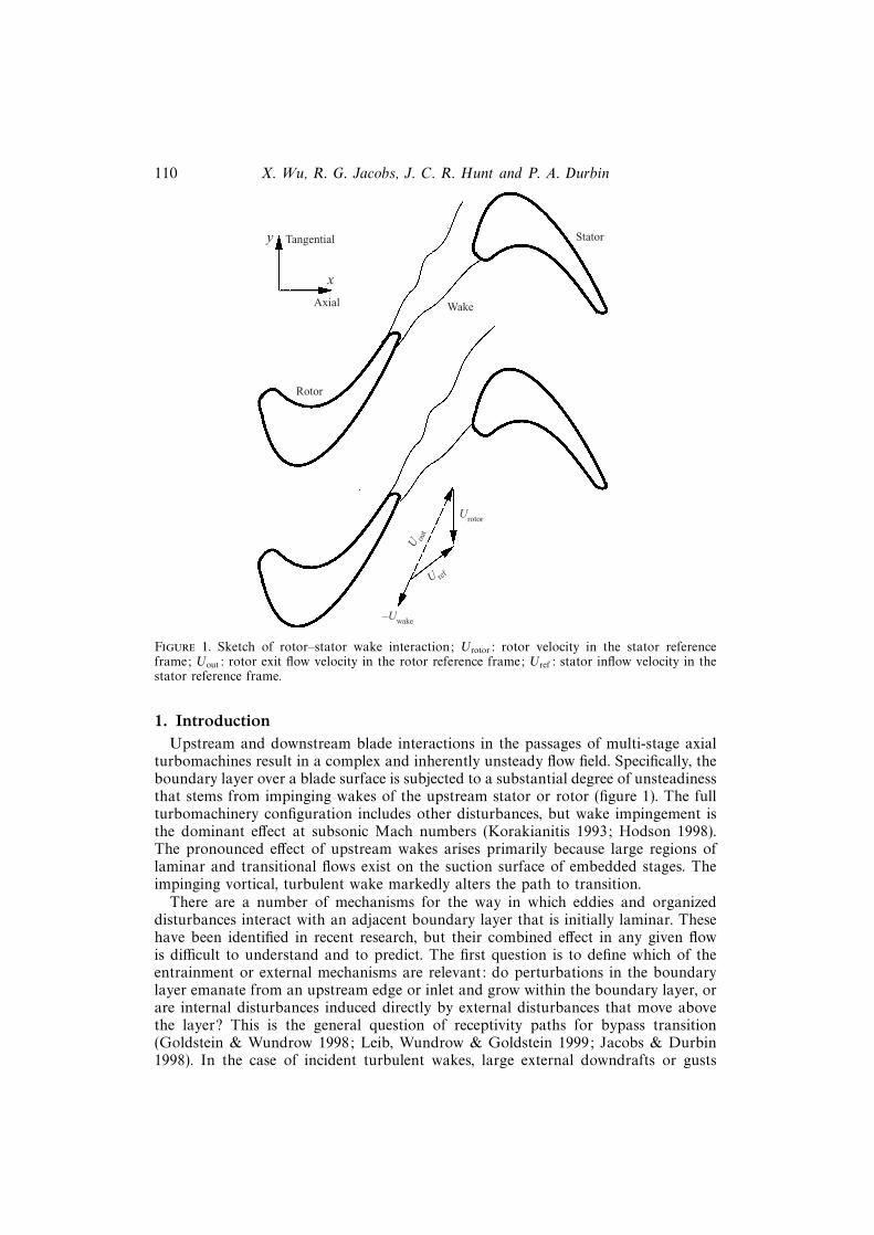
Figure 1. Sketch of rotor–stator wake interaction; Urotor: rotor velocity in the stator referenceframe; Uout: rotor exit flow velocity in the rotor reference frame; Uref : stator inflow velocity in thestator reference frame.

1. IntroductionUpstream and downstream blade interactions in the passages of multi-stage axial

turbomachines result in a complex and inherently unsteady flow field. Specifically, theboundary layer over a blade surface is subjected to a substantial degree of unsteadinessthat stems from impinging wakes of the upstream stator or rotor (figure 1). The fullturbomachinery configuration includes other disturbances, but wake impingement isthe dominant effect at subsonic Mach numbers (Korakianitis 1993; Hodson 1998).The pronounced effect of upstream wakes arises primarily because large regions oflaminar and transitional flows exist on the suction surface of embedded stages. Theimpinging vortical, turbulent wake markedly alters the path to transition.

There are a number of mechanisms for the way in which eddies and organizeddisturbances interact with an adjacent boundary layer that is initially laminar. Thesehave been identified in recent research, but their combined effect in any given flowis difficult to understand and to predict. The first question is to define which of theentrainment or external mechanisms are relevant: do perturbations in the boundarylayer emanate from an upstream edge or inlet and grow within the boundary layer, orare internal disturbances induced directly by external disturbances that move abovethe layer? This is the general question of receptivity paths for bypass transition(Goldstein & Wundrow 1998; Leib, Wundrow & Goldstein 1999; Jacobs & Durbin1998). In the case of incident turbulent wakes, large external downdrafts or gusts

Boundary layer transition induced by passing wakes 111

may be deflected by the vorticity of the layer through the sheltering mechanism ofHunt & Durbin (1999), or they may penetrate the boundary layer to produce locallyamplifying turbulent spots.

The second question concerns how the fluctuations are transformed within theboundary layer and how the layer itself is changed. Instabilities may be triggered atsubcritical Reynolds numbers (Corral & Jimenez 1994) through the action of finite-amplitude disturbances. Only very low level forcing produces transition via Tollmein–Schlichting waves. Moderate or high level forcing leads to transition via formationof localized turbulent spots without Tollmein–Schlichting precursors (Mayle 1991).Once induced, these disturbances grow within the boundary layer, although theirdevelopment may be influenced by modulation of the boundary layer by the free-stream distortion.

The specific receptivity path and internal growth mechanics depend on the particularflow configuration (Hunt & Durbin 1999). However, general questions can be askedwithin the scope of transition induced by localized, convected external disturbancesthat either enter the flow domain abruptly or are rapidly distorted at a leading edge.

There are several mechanisms operative in passing wake-induced bypass transition.The mean wakes distort boundary layer profiles and the wakes are distorted by thewall: does this significantly alter the receptivity and transition processes? Fluctuationsare created as the turbulent wake enters the flow domain: are these the origin of tur-bulent spots, or do their long-wavelength components just modulate the downstreamtransition mechanism? The convected wakes carry free-stream turbulence over theboundary layer: are these free-stream eddies the primary source of transitional spots?The present simulations address these questions.

This paper describes a spatially developing, three-dimensional, time-accurate DNSof boundary layer transition induced by periodically passing wakes (figure 2). Theincident wakes are generated as self-similar free shear flows, but the manner of theirintroduction into the flow domain requires an inevitable distortion near the wall.However, that distortion is well defined and reproducible.

1.1. The connection with some fundamental work on bypass transition

There is now a sizable body of literature from fundamental studies of boundary layerbypass transition due to moderate-amplitude free-stream turbulence. It was realizedby us, only retrospectively, that the problem at hand shares important features withsome of the previous experimental, theoretical and numerical studies. These commoncharacteristics are related to the physical mechanisms leading to the inception ofturbulent spots, their growth through the transition region, and the manner in whichthey maintain the downstream turbulent region.

Experiments by Alfredsson & Matsubara (1996) in a laminar boundary layersubjected to 1.5% and 6% free-stream turbulence showed that during the initialreceptivity and evolution phase, free-stream turbulence induces longitudinal streakswith a fairly periodic, spanwise regularity inside the boundary layer. These structuresgrow downstream both in length and amplitude. Breakdown to turbulent spots wasobserved to occur in the regions where smoke visualization exhibited intensive streaks.The breakdown of streaks often occurs after a wavy motion of the streaks, althoughspots occur locally and abruptly, not via amplification of the wavy motion to the pointof breakdown. The turbulent spots grow in number and size downstream, until theboundary layer becomes fully turbulent. Similar streaky structures inside laminar andtransitional boundary layers were observed by Grek, Kozlov & Ramazanov (1985)and termed puffs; streaks were also found in transitional channel flow (Klingmann


x

uwake

xwake

ywake

vwake

α

Uref

y

L

Ucyl

(a)

x

Uref =1

y

L =1

Ucyl = –0.7 Uref

(b)

0

Figure 2. (a) Layout in the experiments of Liu & Rodi (1991); (b) layout in the present numericalsimulation; the computational domain is defined as 0.1 6 x/L 6 3.5, 0 6 y/L 6 0.8, 0 6 z/L 6 0.2.

1992; Henningson, Lundbladh & Johansson 1993) and in flows experiencing obliquetransition (Berlin, Lundbladh & Henningson 1994).

Previous research on bypass transition induced by free-stream turbulence left opento interpretation the issue of whether intensification and ultimate destruction of thestreaky structures arises from boundary layer internal dynamics, or from forcing byfree-stream eddies. Such ambiguity is primarily due to experimental difficulties infollowing the details of the generation and growth of disturbances because of theirrandomness in space and time.

Figure 3(a–c) illustrates three scenarios observed in the present investigation (see§ 4). In the most interesting case of those drawn in figure 3, inlet wake disturbancesrapidly evolve into puffs similar to those found in Westin et al. (1994) and Alfredsson& Matsubara (1996) and turbulent spots appear downstream. More usually, the puffsdecay as in figure 3(b), at least below the critical Reynolds number Reθ = 200.Turbulent eddies inside the passing free-stream wake impinge on the boundary layerand sometimes interact with its outer part, such as to subject the flow to a rapidlygrowing instability (§ 4). This involves an intensification of the near-wall streakystructures, and eventually the breakdown into young turbulent spots. Figures 3(d)and 3(e) depict two other scenarios in which the flow is subjected to very strongor extremely weak disturbances from the passing wake. Observations concerning the


(a)

Puff

Forcing

Breakdown(young spot)

Turbulentspot

Turbulentstrip

Further decayDecay(b)

(c)

Forcing

Young spotDecay

(d)

Turbulent patch

(e)

Elongated structure with spanwise modulation

z

x

Figure 3. Several possibilities for the downstream propagation of certain types of inlet distur-bances. The sketches represent u′ in an (x, z)-plane very close to the wall: (a) intermediate-strengthdisturbance and strong forcing; (b) intermediate-strength disturbance and weak forcing; (c) inter-mediate-strength disturbance with downstream strong forcing; (d) strong disturbance; (e) very weakdisturbance.

last two instances have been made in the present study through additional numericalsimulations and ‘thought’ experiments (see § 7).

1.2. The connection with some engineering turbomachinery research

Experiments on wake-induced periodic unsteady transition in turbomachinery bladerows were reported by Dring et al. (1982), Dong & Cumpsty (1990), Addison &Hodson (1990), Mayle & Dullenkopf (1991), and Halstead et al. (1997) (see also


the reviews by Mayle 1991 and Walker 1993). Halstead et al. (1996) reported mea-surements in compressors and low-pressure turbines. Their experiments showed thattransition in unsteady, turbomachine boundary layers develops along two different,but coupled, paths. These consist of a wake-induced strip under the convecting waketrajectory, and a path between wakes that is caused by other disturbances. Alongboth paths the boundary layer goes from laminar to transitional to turbulent, withlarge regions of laminar and transitional flow. The switch from the non-wake pathto the wake-induced strip was found to occur in a small fraction of a blade passingperiod. Halstead et al. noted that assumptions of predominantly turbulent boundarylayers on multi-stage turbomachine blading are incorrect.

Although turbine and compressor experiments have indicated that the effects ofwake passing can be substantial and have provided useful guidelines for furtherresearch, the technical complexities involved in obtaining detailed quantitative datafrom rotating turbine/compressor stages make it difficult to isolate physical mecha-nisms. Realizing such complexities, a number of investigators have considered simplergeometries. In the simplest of these (Pfeil, Herbst & Schroder 1983; Liu & Rodi 1991;Orth 1993; Zhong et al. 1998) the unsteady blade row interaction was simulated bysweeping a row of wake-generating cylinders past a flat plate (figure 2). Liu & Rodi(1991) obtained time- and phase-averaged mean and fluctuating streamwise velocityprofiles for four different wake passing frequencies. In their experiments, the Reynoldsnumber was fairly low so that the boundary layer remained laminar over the full platelength when no disturbing wakes were present. They found that the wake-producedturbulent strips grew together and caused the boundary layer to become fully turbu-lent. The streamwise location of the merger moved upstream with increasing wakepassing frequency.

Using experimental data gathered from a similar flow configuration, Orth (1993)concluded that in turbomachinery flows periodically disturbed by passing wakes,the disturbance enters the boundary layer very early on, and convects within itbefore leading to transition. Periodic fluctuation in the velocity profile, as opposedto stochastic fluctuation, does not have a major influence on the transition. This isconsistent with the present study. Orth (1993) also suggested that the location wheretransition takes place is only dependent on inlet turbulence intensity: the passingwake exerts no effect on the process. Our study shows that this needs qualification.Inception of turbulent spots in wake-induced transitional flows is intimately linkedwith turbulent eddies of the travelling free-stream wake. One additional pleasantconnection of the present study with turbomachinery research concerns the recentliquid crystal visualization experiments of Zhong et al. (1998) and Kittichaikarn etal. (1999). This work was communicated to us by Prof. Hodson. Our turbulent spots,as well as their embryo precursors, resemble those observed by Zhong et al. (1998)and Kittichaikarn et al. (1999) to a remarkable degree (see § 3 and § 4).

2. Mathematical and numerical considerations2.1. Problem definition

Consider the evolution of an incompressible flow over a smooth flat plate withupstream wakes passing periodically (figure 2b). The origin of the coordinate systemis at the leading edge of the plate. The wakes are assumed to be generated byimaginary circular cylinders positioned in the plane x = −L and moving in the y-direction at Ucyl, which can be either positive or negative, corresponding to inlet wakes


traversing away from, or towards, the flat plate. The velocity of the flow upstreamof the cylinder is Uref . The cylinders are equally spaced so that they cut throughthe y = 0 plane at a specified passing period T. The characteristic velocity scale isUref , the characteristic length scale is L, the Reynolds number is then Re = UrefL/νwhere ν is the kinematic viscosity of the fluid. Throughout this study Re = 1.5× 105,as in Liu & Rodi (1991). The mean flow properties of the wake are determined byfree-stream velocity, cylinder velocity and cylinder diameter.

The computational domain for the DNS is defined as 0.1 6 x/L 6 3.5, 0 6 y/L 60.8, and 0 6 z/L 6 0.2. The inlet momentum thickness Reynolds number is Reθ = 80in all the simulations. Unless otherwise noted, all velocities are normalized by thereference velocity Uref and all lengths by the characteristic length scale L.

2.2. Governing equations and notation

Mass and momentum conservation is enforced for flow over the flat plate by solvingthe full time-dependent, mass-conservation and Navier–Stokes equations in Cartesiancoordinates,

div u = 0, (1)

∂u

∂t+ div (uu) = −1

ρgrad p+ div

{1

Re

[grad u+ (grad u)S

]}, (2)

where u is the velocity vector with Cartesian components (u, v, w) or ui, i = 1, 2, 3.Superscript S denotes transpose. The equations are in non-dimensional form.

In this paper, time-averaging is represented by · . Averaging at a particular phase,tmnT = mT + nTT, is denoted by 〈·〉, where m is any integer and 0 6 nT 6 1 is thefraction of the wake passing period. For example, the phase-averaged mean velocitycomponents are evaluated as

〈ui〉(tnT) =1

M

M∑m=1

ui(tmnT), (3)

where M is the total number of periods within which phase averaging is per-formed. Averaging over the homogeneous spanwise z-direction is implied in bothtime-averaging and phase-averaging. Time-averaged and phase-averaged mean veloc-ities are related via ui = 〈ui〉. Thus the instantaneous velocity can be decomposedas

ui = 〈ui〉(tnT) + u′i(tnT) = ui + ui(tnT) + u′i(tnT), (4)

where ui(tnT) = 〈ui〉(tnT) − ui is the periodic velocity fluctuation with respect tothe time-averaged mean, and u′i(tnT) is the true stochastic turbulence fluctuation.

Consequently, the time-averaged Reynolds stresses 〈u′iu′j〉 can be calculated as

〈u′iu′j〉 =

∫ 1

0

⟨[ui − 〈ui〉(tnT)

][uj − 〈uj〉(tnT)

]⟩dnT. (5)

2.3. Inflow and other boundary conditions

For all the simulations described in this paper, the height of the computationaldomain 0.8L is approximately 200δ at the inlet x = 0.1L, 20δ in the middle of theplate x = 1.75L, and 11δ at the exit x = 3.5L. δ(x) is the 99% boundary layerthickness. The width of the computational domain 0.2L is equivalent to 40δ at theinlet, 5δ in the middle of the plate and 3δ at the exit.


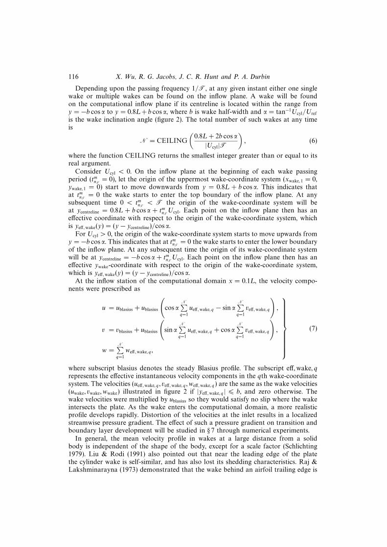
Depending upon the passing frequency 1/T, at any given instant either one singlewake or multiple wakes can be found on the inflow plane. A wake will be foundon the computational inflow plane if its centreline is located within the range fromy = −b cos α to y = 0.8L+ b cos α, where b is wake half-width and α = tan−1Ucyl/Uref

is the wake inclination angle (figure 2). The total number of such wakes at any timeis

N = CEILING

(0.8L+ 2b cos α

|Ucyl|T), (6)

where the function CEILING returns the smallest integer greater than or equal to itsreal argument.

Consider Ucyl < 0. On the inflow plane at the beginning of each wake passingperiod (tmnT = 0), let the origin of the uppermost wake-coordinate system (xwake, 1 = 0,ywake, 1 = 0) start to move downwards from y = 0.8L + b cos α. This indicates thatat tmnT = 0 the wake starts to enter the top boundary of the inflow plane. At anysubsequent time 0 < tmnT < T the origin of the wake-coordinate system will beat ycentreline = 0.8L + b cos α + tmnTUcyl. Each point on the inflow plane then has aneffective coordinate with respect to the origin of the wake-coordinate system, whichis yeff ,wake(y) = (y − ycentreline)/cos α.

For Ucyl > 0, the origin of the wake-coordinate system starts to move upwards fromy = −b cos α. This indicates that at tmnT = 0 the wake starts to enter the lower boundaryof the inflow plane. At any subsequent time the origin of its wake-coordinate systemwill be at ycentreline = −b cos α + tmnTUcyl. Each point on the inflow plane then has aneffective ywake-coordinate with respect to the origin of the wake-coordinate system,which is yeff ,wake(y) = (y − ycentreline)/cos α.

At the inflow station of the computational domain x = 0.1L, the velocity compo-nents were prescribed as

u = ublasius + ublasius

(cos α

N∑q=1

ueff ,wake, q − sin αN∑q=1

veff ,wake, q

),

v = vblasius + ublasius

(sin α

N∑q=1

ueff ,wake, q + cos αN∑q=1

veff ,wake, q

),

w =N∑q=1

weff ,wake, q ,

(7)

where subscript blasius denotes the steady Blasius profile. The subscript eff, wake, qrepresents the effective instantaneous velocity components in the qth wake-coordinatesystem. The velocities (ueff ,wake, q , veff ,wake, q , weff ,wake, q ) are the same as the wake velocities(uwake, vwake, wwake) illustrated in figure 2 if |yeff ,wake, q | 6 b, and zero otherwise. Thewake velocities were multiplied by ublasius so they would satisfy no slip where the wakeintersects the plate. As the wake enters the computational domain, a more realisticprofile develops rapidly. Distortion of the velocities at the inlet results in a localizedstreamwise pressure gradient. The effect of such a pressure gradient on transition andboundary layer development will be studied in § 7 through numerical experiments.

In general, the mean velocity profile in wakes at a large distance from a solidbody is independent of the shape of the body, except for a scale factor (Schlichting1979). Liu & Rodi (1991) also pointed out that near the leading edge of the platethe cylinder wake is self-similar, and has also lost its shedding characteristics. Raj &Lakshminarayna (1973) demonstrated that the wake behind an airfoil trailing edge is


similar to that of a two-dimensional cylinder wake. Invoking self-similarity allows thewake introduced at the inlet to be obtained more simply than by actually computinga real cylinder wake.

The turbulent wake velocities (uwake, vwake, wwake) appearing in (7) were generatedfrom a separate precomputation of a temporally decaying, self-similar plane wake,following the work of Moser, Rogers & Ewing (1998) and Ghosal & Rogers (1997) .In a temporally decaying wake, the flow is statistically homogeneous in the streamwiseand spanwise directions, and inhomogeneous in the cross-stream direction. The initialconditions for the temporally decaying plane wake simulation were generated from aturbulent channel flow simulation at Reynolds number 3300 based on the centrelinemean velocity and channel half-height. The procedure involved taking two realizationsof half-channel flow and ‘fusing’ them together. Physically this corresponds to asituation in which two half-channel flows exist on either side of a rigid plate andthe plate is instantaneously removed. This simulation was performed on a grid sizeof (65, 128, 128) using an LES code (Wu & Squires 1997). The grid sizes used byGhosal & Rogers (1997) and Moser et al. (1998) were (65, 48, 16) and (512, 195, 128),respectively.

Mean flow and turbulence statistics of the simulated plane wake are presented infigure 4. All velocities in the figure are normalized by the maximum mean velocitydeficit uwake,max; lengths are normalized by the wake half-width b. Following Ghosal& Rogers (1997) , the half-width b is defined as the distance between the two points atwhich the mean velocity deficit is 50%uwake,max. This is slightly larger than the distancebetween the wake centreline and the first point with effectively zero mean velocitydeficit. Figure 4(a) shows that mean velocity profiles obtained at the three differentinstants (indicated in the caption by their descending maximum velocity deficits)collapse. These mean profiles are also in excellent agreement with experimentalmeasurements and the data correlation of Schlichting (1979), i.e. uwake/uwake,max =[1 − (ywake/1.1338b)1.5]2. This demonstrates that the simulated wake has reached aself-similar state and that the mean flow has lost its memory of the initial condition.At these and subsequent instants, the product of the wake width and maximum deficitremains constant.

Figure 4(b, c) show the r.m.s. turbulence intensities for the decaying plane wakeat the same three instants. Turbulent shear stress profiles are given in figure 4(d).The turbulence intensities obtained by Moser et al. (1998) and Ghosal & Rogers(1997) have two distinct features: double peaks occur in the streamwise component,and the wall-normal component is slightly higher than the spanwise component.In addition, the results of Ghosal & Rogers show that unlike the mean flow andthe anti-symmetrical Reynolds shear stress profiles, the turbulence intensities arenot self-similar as time proceeds. It is evident from figure 4(b–d) that the presentprecomputation reproduced all these essential features. Figure 4(e) presents profilesof the rate of turbulence kinetic energy dissipation. Spanwise energy spectra of theturbulence kinetic energy are given in figure 4(f) for completeness. Note that theresults in figure 4 are presented in the wake-coordinate system (see figure 2). Thefluctuating wake velocities obtained from the precomputation are rescaled by thewake maximum deficit uwake,max and half-width b before they are applied to (7).Using the experimental correlation of Schlichting (1979) for far wakes, at x/L = 0.1uwake,max = 0.14Uref and b ≈ 0.1L for the present flow conditions.

At the top surface of the computational domain the following boundary conditionswere applied: v = vblasius, ∂u/∂y = ∂v/∂x, and ∂w/∂y = ∂v/∂z. This is artificial, butgiven the substantial distance between the top surface and the wall, the effect of the


(e)0.20

0.16

0.12

0.08

0.04

0–2 –1 0 1 2

y/b

εb/u

3 wak

e, m

ax

( f )

10–10

1 10 100 1000

kzb

(c)

0.8

0.6

0.4

0.2

0–2 –1 0 1 2

y/b

(d )0.10

0.06

0.02

–0.02

–0.06

–0.1–2 –1 0 1 2

y/b

(a)

0.1

–0.1

–0.3

–0.5

–0.7

–1.1–2 –1 0 1 2

y/b

(b)

0.8

0.6

0.4

0.2

0–2 –1 0 1 2

y/b

10–8

10–6

10–4

10–2

100

E/b

u2 w

ake,

max

–0.9

u wak

e/u w

ake,

max

u′21/

2

wak

e, w

′21/

2

wak

e/u w

ake,

max

u′ wak

e v′ w

ake/

u2 w

ake,

max

v′21/

2

wak

e/u w

ake,

max

Figure 4. Characteristics of the simulated temporally decaying plane wake for the generation ofinflow turbulence: ——, uwake,max = 0.12; · · · · ·, uwake,max = 0.10; – – – –, uwake,max = 0.08; �, plane

cylinder wake of Schlichting (1979); — ·—, E ∝ k−5/3z law. (a) Mean velocity; (b) streamwise and

spanwise fluctuations; (c) wall-normal fluctuations; (d) turbulent shear stress; (e) viscous dissipationrate of turbulence kinetic energy; (f) spanwise spectrum of turbulence kinetic energy.

top boundary condition on boundary layer development should be extremely small.At the exit of the computational domain, convective boundary conditions were used.Mass flux at the inflow plane was made constant in time by rescaling the velocitiesobtained from (7), and corrections to the velocities at the exit plane are also madeto ensure global mass conservation. Periodic boundary conditions were applied in thehomogeneous, spanwise z-direction; u = 0 was applied on the wall.


(c)2.0

1.5

1.0

0.5

0 0.02 0.04 0.06 0.08y

⟨v′2

⟩1/2,

+

(d )2.0

1.5

1.0

0.5

0 0.02 0.04 0.06 0.08y

(a)0.8

0.6

0.4

0.2

010–1

(b)3

2

1

0 0.02 0.04 0.06 0.08

⟨u′2

⟩1/2,

+⟨w

′2⟩1/

2,+

10–210–310–410–5

1.0

u

Figure 5. Resolution check: symbols, baseline case with ∆x+x= 3 = 24 (∆x+

x= 1 = 18.3) and ∆z+x= 3 = 11

(∆z+x= 1 = 8.4): e, during transition x = 1.0; �, after transition x = 3.0; — —, spanwise resolution

refined by 50%; · · · · ·, streamwise resolution coarsened by 50%.

2.4. Numerical method

The numerical scheme for the DNS is a parallelized version (by Charles D. Pierce atStanford) of the method used by Akselvoll & Moin (1996) and Pierce & Moin (1998).Convection and diffusion terms that involve only derivatives in the wall-normaldirection are treated implicitly, whereas all other terms are treated explicitly. Allspatial derivatives are approximated with a second-order central difference scheme.A third-order Runge–Kutta scheme (Spalart, Moser & Rogers 1991) is used forterms treated explicitly and a second-order Crank–Nicolson scheme is used for termstreated implicitly. The fractional step method is used to remove the implicit pressuredependence in the momentum equations. Further details can be found in Akselvoll& Moin (1996). For parallel computation the computational domain is decomposedin two directions whereas a third direction is complete. When solving the Poissonequation using fast transforms, a transpose is necessary to switch the un-decomposeddirection. Scalable parallelization is achieved using message passing interface (MPI)libraries.

2.5. Computational details and resolution check

The governing equations are solved on a rectangular staggered grid. The grid spacingsare uniform in the streamwise and spanwise directions.

Simulation results to be presented in the following sections were obtained on a(1024, 400, 128) grid in the streamwise, wall-normal and spanwise directions, respec-


(c) t/4 = 32.9

0.6

0.4

0 0.5 1.0 1.5x

0.2

y

2.0 2.5 3.0 3.5

wake 3

wake 2wake 1

(b) t/4 = 32.7

0.6

0.4

0 0.5 1.0 1.5

0.2

y

2.0 2.5 3.0 3.5

wake 3

wake 2wake 1

(a) t/4= 32.5

0.6

0.4

0 0.5 1.0 1.5

0.2

y

2.0 2.5 3.0 3.5

wake 3

wake 2wake 1

Figure 6. Contours of u over one (x, y)-plane.

tively. The total of 52.4 million grid points is one of the largest that has ever beenreported: compare to 11.0 million, 6.2 million and 17.3 million used by Spalart (1988),Yang, Spalart & Ferziger (1992) and Rai & Moin (1993), respectively.

In terms of viscous wall units based on the time-averaged local friction velocityafter transition, ∆x+

x= 3 = 24 and ∆z+x= 3 = 11. When measured using a friction velocity

during transition, ∆x+x= 1 = 18.3 and ∆z+

x= 1 = 8.4. At the exit, there are 16 pointsdistributed along the wall-normal direction below y+ = 9, and a total of 191 pointsbelow y = δ. The resolution used in Spalart (1988) was ∆x+ ≈ 20±1, ∆z+ ≈ 6.7±0.34,with 10 points within 9 wall units.

In order to check the adequacy of the streamwise and spanwise grid resolution,two complete additional simulations were performed. It was difficult to use a grid sizelarger than (1024, 400, 128) due to memory constraints of the computer. Therefore, inthe first additional simulation the spanwise dimension of the computational domainwas reduced from 0.2L to 0.15L, which is equivalent to 30δ at the inlet, 3.94δ in themiddle of the plate and 2.18δ at the exit. Even such a reduced spanwise dimensionis still sufficiently wide and we therefore assume most of the differences, if any,between the two sets of results are due to the spanwise grid resolution change from∆z+

x= 1 = 8.4 to ∆z+x= 1 = 6.3. In the second additional simulation, the number of grid

points in the streamwise direction was reduced by 50% from 1024 to 768. Except forthese changes, all the other parameters were kept the same as the baseline simulation.Results from the resolution check are presented in figure 5. Figure 5(a) compares thethree sets of mean velocity profiles at two streamwise stations: the first, at x = 1.0,is in the transitional region; and the second, at x = 3.0, is in the turbulent region.


(c) t/4 = 32.9

0.6

0.4

0 0.5 1.0 1.5x

0.2

y

2.0 2.5 3.0 3.5

wake 3

wake 2wake 1

(b) t/4 = 32.7

0.6

0.4

0 0.5 1.0 1.5

0.2

y

2.0 2.5 3.0 3.5

wake 3

wake 2wake 1

(a) t/4 = 32.5

0.6

0.4

0 0.5 1.0 1.5

0.2

y

2.0 2.5 3.0 3.5

wake 3wake 2

wake 1

Figure 7. Contours of v over one (x, y)-plane. In this and subsequent similar figures, negativevalues are contoured by solid lines; positive values are contoured by dashed lines.

The curves show good numerical resolution. Figures 5(b), 5(c) and 5(d) comparethe streamwise, wall-normal and spanwise r.m.s. turbulent intensities, respectively.Differences among the three simulations are small. Additional resolution checks canbe found in § 5. In addition to these resolution checks, we also build confidence on oursimulation through extensive comparison, presented in § 5, with well-accepted DNSand experimental data. Comparison with the resolution used in previous channel flowturbulent spot simulations (e.g. Henningson & Kim 1991) gives further confidence thatthe present resolution is adequate. Years of turbulence simulation research at StanfordUniversity has shown that, despite the slow convergence rate with grid refinement,second-order central differencing has several attractive features. It is energy conservingand does not carry inherent numerical diffusion, as do many high-order upwind biasedschemes.

The time step was fixed to be dt = 10−3T=0.00167L/Uref , which is equivalent to0.59 ν/u2

τ, x= 3. Initial velocities were set to the laminar Blasius profile. The flow wasthen allowed to evolve for 20 wake passing periods (20 000 dt), and statistics werethen collected for another 20 wake passing periods. Phase averaging was performedby dividing each pass period into 50 equal subdivisions. The computation was carriedout on the scalable parallel Cray T3E at the Pittsburgh Supercomputing Center, usingup to 512 processors.

3. Visualization of a matured turbulent spotAt the beginning of each period tmnT = 0, the passing wake starts to enter the

computational inflow plane at the top boundary y = 0.8L. Since the cylinder travels


(a)0.10

0.05

0.625 0.750x

0.00

z

0.875 1.000 1.125

(b)

Flow

Figure 8. (a) Contours of u′ at t/T = 32.5 over the (x, z)-plane y = 7.38 × 10−4 (y+ = 5.4 atx = 1.75) – negative u′ represented by dashed lines; (b) visualization from the experiments of Zhonget al. (1998).

at −0.7Uref , it takes 1.143L/Uref or 0.684T before the wake reaches the flat plate.After entering the computational domain, the wake is advected at the referencevelocity Uref in the free stream and interacts with the boundary layer in the near-wallregion. An important grid resolution requirement is that it be adequate to ensure thatno vorticity is spuriously left in the free stream after the wake has passed.

An overall view of the wake evolution as it is advected along the plate and thelaminar to turbulent transition can be seen in figures 6 and 7. Figure 6 presentscontours of instantaneous streamwise velocity over one random (x, y)-plane at threeconsecutive instants: t = 32.5T, 32.7T and 32.9T. It is seen from the figure that inthe free stream the wake angle remains the same at all the three instants, and thatthere is no residual velocity gradient left by the passing wake. The small effects of theupper boundary show that the computational domain is sufficiently high compared tothe boundary layer thickness. Between the wakes the near-wall velocity contours fromthe inlet to x ≈ 1.0 are straight, indicating that the flows in these moving regions arepredominantly laminar. Beyond x = 1.75 the contours are chaotic in the near-wallregion at all the instants, and there is also apparent thickening in the boundary layer.This indicates that laminar-to-turbulent transition has been nearly completed.

Figure 7 presents contours of instantaneous wall-normal velocity v at the samelocations and instants as in figure 6. The wall-normal velocity inside the wake issignificantly larger than that in the free stream of a normal laminar or turbulentboundary layer because of the wake angle α. The figure shows that downstream


0.2

0.1

1.75 2.00 2.25x

0

z

2.50 2.75

Figure 9. Contours of u′ at t/T = 32.5 over the (x, z)-plane of y = 7.38 × 10−4 (y+ = 5.4 atx = 1.75) showing turbulent streaks in the turbulent region – negative u′ represented by darkercontours.

Wall

Speaker

y

x

Ub

Breakdown (source)

U

UaA

y

xAUb–Ua

Breakdown (source)

z

x

Wall

y

x

Ub

Breakdown

U

UaA

y

xA

Ub–UaBreakdown

z

x

Wall Wall

Figure 10. One possible reconciliation of the spot arrowhead direction found inthe present study with that in previous boundary layer studies.

0.05

0.03

0.7 0.8 0.9x

y

1.0 1.1

0.01

1.2

Figure 11. Side-view of the turbulent spot at t/T = 32.5 over the (x, y)-plane of z = 0.03: ——,−0.20Uref < v′ < −0.01Uref ; - - - -, 0.01Uref < v′ < 0.20Uref ; increment 0.005Uref .

of x ≈ 2.0 the instantaneous wall-normal velocity is chaotic near the wall, withsubstantial magnitude all the time, as would be found inside a turbulent boundarylayer. It is interesting to note that, upstream of x ≈ 1.75L, an isolated spot nearthe wall containing large-amplitude and chaotic vertical velocities is developing on


(c) t/4= 32.90.2

0.1

0 0.5 1.0 1.5x

z

2.0 2.5 3.0 3.5

(b) t/4 = 32.70.2

0.1

0 0.5 1.0 1.5

z

2.0 2.5 3.0 3.5

(a) t/4 = 32.50.2

0.1

0 0.5 1.0 1.5

z

2.0 2.5 3.0 3.5

Figure 12 (a–c). For caption see facing page.

the upstream side of the free-stream wake. It can be seen from the contours that asthe spot propagates downstream, its streamwise dimension lengthens. The evolutionof this particular turbulent spot, as well as its connection to the overall unsteadyboundary layer transition, will be examined in the remainder of this subsection.

Figure 8(a) provides a close-up plan view of the turbulent spot indicated byfigure 7(a). Shown in the figure are contours of u′ at t = 32.5T over the (x, z)-plane of y = 7.38×10−4. The spot has an arrowhead shape pointing upstream, withstreamwise elongation. Because u′ represents turbulence fluctuations with respect tothe phase-averaged mean, the contours are predominantly positive inside the spot. Ifu′ is computed with respect to a conditional mean, averaged only inside the spot, therewill be both positive and negative fluctuations. This can also be inferred from thehigh-speed and low-speed streaks inside the spot in figure 8(a). Figure 8(b) presentsa flow visualization picture obtained by Zhong et al. (1998) in an experimentalconfiguration similar to ours (figure 2b). Good agreement between the DNS spot andthe experimental visualization is evident. Figure 9 shows contours of u′ at the sametime and (x, z)-plane as in figure 8(a), but within a further downstream, fully turbulentregion. The most distinctive feature found in the figure is the existence of low- andhigh-speed streaks. These streaks and their associated streamwise vortices have beenrecognized as a signature of fully developed near-wall turbulence (Hamilton, Kim &


( f ) t/4 = 33.60.2

0.1

0 0.5 1.0 1.5x

z

2.0 2.5 3.0 3.5

(e) t/4 = 33.5

0.2

0.1

0 0.5 1.0 1.5

z

2.0 2.5 3.0 3.5

(d ) t/4 = 33.4

0.2

0.1

0 0.5 1.0 1.5

z

2.0 2.5 3.0 3.5

Figure 12. Visualization of spot growth and transition to turbulence using v′ over the (x, z)-plane of y = 7.38× 10−4 (y+ = 5.4 at x = 1.75); contours represent 0.005Uref 6 |v′| 6 0.2Uref withincrement 0.005Uref .

Waleffe 1995). The commonly accepted characteristic wavelength of such streaks isabout 100 wall units. The entire spanwise dimension in figure 9 is about 1400 wallunits. Such turbulent streaks should not to be confused with the puffs existing in thelaminar region prior to the occurrence of turbulent spots, as drawn in figure 3.

Our turbulent spot and that of Zhong et al. (1998) have an arrowhead pointingupstream, in the reverse direction to that reported in many previous boundary layerstudies (Henningson, Spalart & Kim 1987; Jahanmiri, Prabhu & Narasimha 1996).This discrepancy is too glaring to be left uncommented on.

Figure 10 depicts a simple rationale for the difference. The breakdown fluid parcelscontain the ‘source’ of turbulence, which is spread to form a spot as the parcelsthemselves are convected downstream. In many previous boundary layer turbulentspot studies breakdown takes place near the wall, where the local convection velocityis small. At the position, A, located higher above the wall than the source, theturbulent fluid parcels travel downstream relative to the source. At any given instantfluid parcels at smaller xA have a longer time to spread laterally, thus forming anarrowhead pointing downstream.


Breakdown provoked by free-stream turbulence occurs in the outer part of thelayer where the local convection velocity is large (see § 4 for further discussion). Inthe reference frame of observer A, nearer to the wall than the breakdown location,the highly turbulent breakdown fluid parcels are convected downstream. At any giveninstant, fluid parcels at larger xA have had longer to spread laterally, thus forming anarrowhead pointing upstream. Alternatively, in the frame of reference of the source,the boundary layer flow is increasingly in the −x-direction as the wall is approached.Thus the spot is sheared towards the upstream direction near the wall: the verticalsection in figure 11 illustrates this structure.

Evolution of a turbulent spot and the process of unsteady periodic transition isportrayed in figure 12. Presented in this figure are visualizations of the instantaneouswall-normal fluctuation v′ over the (x, z)-plane, y = 7.38× 10−4, which is equivalentto y+

x= 1.75 = 5.4. A total of six consecutive realizations are given from t = 32.5Tto t = 33.6T, covering more than a full wake passing period. In the figure, thebackground is used to represent negligible fluctuations with −0.005 6 v′ 6 0.005.Other contours represent stronger fluctuations 0.005 < |v′| < 0.2 with an incrementof 0.005. Note that the spanwise dimension in figure 12 has been magnified by afactor of four in order to show the full streamwise dimension. The spot appearing infigure 12(a) is the same as that presented in figure 8(a), except that the contours arenow drawn using v′. Because of the enlarged z-dimension, the spot dimensions aredistorted. Their real physical shape is as in figure 8(a).

In figure 12(b) a small patch of large turbulent fluctuations exists near the upperboundary (z ≈ 0.2, x ≈ 1.0). This is part of the wing tip of the turbulent spot nearthe lower boundary, extended via the periodic boundary condition in the spanwisedirection. From t = 32.5T to 32.7T the arrowhead of the turbulent spot broadens,but is still pointing upstream. In the meantime the flank of the spot becomes sharper,making a well-defined angle with respect to the flow direction. As the wing tipexpands, more fluctuations stronger than the background level are seen to appearnear z = 0.2 as well. Along the z = 0 boundary, the downstream turbulent regionretreats from x ≈ 1.65 at 32.5T to x ≈ 1.75 at 32.7T.

At t = 32.7T the next wake starts to touch the flat plate. Large turbulencefluctuations advected into the near-wall region of the computational domain by thewake can be seen in figure 12(c) near x = 0.25. These fluctuations decay rapidlyso that in figure 12(d) they have entirely disappeared. This provides evidence thatturbulent spots are not produced immediately where impact occurs.

From t = 32.7T to 32.9T, the shape of the turbulent spot transforms from awell-defined wedge to a two-dimensional strip. This process occurs through a rapidincrease in the angle which the flank makes with the streamwise direction. Eventuallythe arrowhead shape disappears, resulting from a tendency towards equalization ofthe dimensions of the leading and trailing edges of the spot.

Formation of a full two-dimensional strip, and catching up the downstream tur-bulent region by the strip, are shown in figure 12(d). The two-dimensional strip doesnot extend over the whole spanwise dimension until t = 33.4T, nearly 0.9 passingperiod after the appearance of the spot in figure 12(a). Relative to the given pass-ing frequency, the evolution from isolated turbulent spots to a full two-dimensionalstrip is rather gradual. Prior to being caught by the turbulent strip, the continuouslyturbulent region had moved to x ≈ 2.4L; through the act of being caught, the contin-uously turbulent region jumps back to 1.6L, restoring its position of figure 12(a). Thetransition cycle is begun anew by the emergence of two small turbulent spots nearx ≈ 0.9L in figure 12(e). Figure 12(f) shows the state of these two young turbulentspots after another 0.1 passing period.


(a)

0.10

0.05

0.0 0.25x

z

0.5 0.75

(b)

Flowx

z

0.15

0.20

Figure 13. ‘Puff’ prior to the emergence of turbulent spot: (a) u′ at t/T = 33.2 over the (x, z)-planeof y = 7.38× 10−4 (y+ = 5.4 at x = 1.75). (b) Visualization from the experiments of Kittichaikarnet al. (1999).

4. The search for the origin of a young turbulent spotWe have argued in § 1 and § 3 that inlet disturbances develop into streaky structures

(puffs) inside the boundary layer. Selective amplification of the puffs in the transitionalregion occurs when certain types of free-stream wake eddies interact with boundarylayer flow. Breakdown starts near the boundary layer edge. We are now ready toprovide supportive evidence for this argument.

Figure 13(a) demonstrates the existence of streaky structures in the transitionalregion. Shown in the figure are u′ contours at t = 33.2T over the same (x, z)-plane as in figure 12. This particular instant is 0.3T prior to the emergence ofyoung spots in figure 12(e). The elongated positive and negative u′ contours resem-ble the puff sketched in figure 3, and are essentially the same as those observedby Alfredsson & Matsubara (1996) in a boundary layer under continuous free-stream turbulence. Figure 13(b) presents one interesting flow visualization pictureobtained by Kittichaikarn et al. (1999) that compares favourably with our simulation.The three streaky structures are precursors of turbulent spots. Additional visualiza-tions show the occurrence of three well-defined turbulent spots some time followingfigure 13(b).

Figure 14 follows the three puffs of figure 13(a) through their earlier history. It startswith their inception, near the inlet, and follows them to their ultimate breakdown


(c) t/4 = 33.10.20

0.15

0 0.25x

z

0.50 0.75

0.10

0.05

(b) t/4 = 32.90.20

0.15

0 0.25

z

0.50 0.75

0.10

0.05

(a) t/4 = 32.8

0.20

0.15

0 0.25

z

0.50 0.75

0.10

0.05


near x = 1.0. That is the point of the emergence of young spots in figure 12(e). Inthis figure the contour plots of v′ have the threshold level reduced by a factor often compared to figure 12 (from 0.005 to 0.0005). Near-wall inlet wake disturbancesshown in figure 14(a) rapidly evolve into three patches in figure 14(b). Each of thesethree patches is made of elongated structures with upward and downward motions,suggesting an association with streamwise vortices. Figure 14(c) shows that the toppuff (near z = 0.175) and lower puff (near z = 0.025) decay from 32.9T to 33.1T,whereas the middle puff (near z = 0.1) intensifies. Attenuation or amplification ofthe near-wall puff is dependent upon the type of forcing from free-stream eddies.Figure 15 illustrates such forcing. Figure 15(a) shows u′ in an (x, y)-plane cut throughthe centre of the top puff, at an instant midway between figure 14(b) and figure 14(c).The time-averaged boundary layer thickness in this region is about 0.006. Positiveu′ are found behind the wake inside the boundary layer (0.25 < x < 0.4), implyingthe absence of inflectional instability. Figure 15(c) shows u′ in an (x, y)-plane cutthrough the centre of the lower puff. Again, positive u′ is evident. The lack of forcingthrough inflectional instability in figures 15(a, c) corresponds to the decay of the top


( f ) t/4 = 33.50.20

0.15

0.50 0.75x

z

1.00 1.25

0.10

0.05

(e) t/4 = 33.40.20

0.15

0.50 0.75

z

1.00 1.25

0.10

0.05

(d) t/4 = 33.30.20

0.15

0.50 0.75

z

1.00 1.25

0.10

0.05

Figure 14. Visualization of the evolution of puffs and breakdown to young turbulent spots usingv′ over the (x, z)-plane of y = 7.38× 10−4 (y+ = 5.4 at x = 1.75); 0.0005Uref 6 |v′| 6 0.008Uref withincrement 0.0005.

and lower puff shown in figure 14(c). Figure 15(b) presents contours of u′ in an(x, y)-plane cut through the centre of the middle puff. Evident from the figure arethe negative u′ contours in the region where free-stream wake eddies interact withboundary layer flow. This corresponds to the amplification of the middle puff seen infigure 14(c).

Figure 14(d–f) shows variations of the three puffs before breakdown. The trendtoward attenuation of the top puff is reversed. This is because the free-stream forcingshown in figure 16(a) is of the opposite sign to that in figure 15(a). u′ is stronglynegative. Strong negative u′ is also seen in figure 16(b). Under such forcing, the topand middle puff break up at t = 33.5T. In contrast, figure 16(c) shows there is veryweak forcing in the lower puff. This corresponds to its monotonic decay as seen infigure 14(b–f). Figure 17 visualizes the evolution of the three puffs by way of contoursof streamwise fluctuations.

Figure 18 shows the breakdown using contours of u′. Again, the three (x, y)-planesz = 0.175, 0.11 and 0.025 cut through the centres of the three puffs. Due to thenegative u′, the boundary layers in figure 18(a) and figure 18(b) have inflectional


(c) z = 0.025, t/4 = 33.0

0.25 0.5x

y

0.75 1.0

0.10

0.08

0.06

0.04

0.02

(b) z = 0.11, t/4 = 33.0

0.25 0.5

y

0.75 1.0

0.10

0.08

0.06

0.04

0.02

(a) z = 0.175, t/4 = 33.0

0.25 0.5

y

0.75 1.0

0.10

0.08

0.06

0.04

0.02

Figure 15. Visualization of the forcing by free-stream eddies through localized instability using u′over three (x, y)-planes at t/T=33.0; 0.02Uref 6 |u′| 6 0.34Uref with increment 0.04.

profiles. The wavy structures in the velocity field are the signature of their instability.Figure 18(b) suggests that breakdown occurs first in the outer part of the layer. Whenbreakdown takes place, the negative streamwise fluctuations are replaced by positivefluctuations (compare figure 18(b) and figure 19(b) at x = 1.0). A turbulent spotis made of predominantly positive u′ (see figure 8a), thus high local skin friction.Near the downstream end of the turbulent spot, positive u′ of the spot collides withnegative u′ associated with the forcing (see figure 19b at x = 1.05). Continuity thusresults in a high positive wall-normal fluctuation v′ in this region. The strong upwardmotion near the downstream end of the spot results in an overhang, which is clearlyvisible in figure 7(c).

One final observation to be made is that figure 18(b) shows more conclusivelythat breakdown starts from the outer layer than figure 18(a). Our reasoning in § 3concerning the arrowhead direction of the spot associated with the middle puff is thatit should have a more well-defined arrowhead pointing upstream than the top one.This is indeed the case. See the two young spots in figure 12(f) and note again thatthe spanwise dimension has been enlarged by a factor of four.


(c) z = 0.025, t/4 = 33.4

0.75 1.00x

y

1.25 1.50

0.10

0.08

0.06

0.04

0.02

(b) z = 0.11, t/4 = 33.4

0.75 1.00

y

1.25 1.50

0.10

0.08

0.06

0.04

0.02

(a) z = 0.175, t/4 = 33.4

0.75 1.00

y

1.25 1.50

0.10

0.08

0.06

0.04

0.02

Figure 16. Visualization of the forcing by free-stream eddies through localized instabilityusing u′ over three (x, y)-planes at t/T=33.4; 0.02Uref 6 |u′| 6 0.34Uref with increment 0.04.

5. Time-averaged boundary layer propertiesTime-averaged boundary layer integral parameters are presented in figure 20. In

addition to the laminar Blasius solution, two sets of DNS results are shown: thesimulation with ∆z+

x= 3 = 11 and an additional simulation with ∆z+x= 3 = 8.25. The

laminar-flow momentum thickness Reynolds number Reθ is 80 at the inflow station(x = 0.1). This is dictated by the assumption that the Blasius boundary layer isinitiated from the leading edge with the prescribed length Reynolds number. Atthe exit of the computational domain (x = 3.5) the turbulent boundary layer hasReθ = 1120. It is seen from the figure that upstream of x ≈ 0.75 the simulationsfollow the Blasius solution quite nicely with only very small deviations. The minordifferences are due to the impact of the wake on the flat plate. Onset of transitionstarts at about x ≈ 0.7 and by x ≈ 2.0 the shape factor has dropped from 2.59to 1.45. Further downstream the shape factor remains nearly the same, decreasingonly slightly from 1.45 to 1.42 at the exit. Coles’ (1956) correlation shows that in aturbulent boundary layer the shape factor drops from 1.48 at Reθ = 600 to 1.44 atReθ = 1100.

Quantitative time-averaged skin-friction data are not available in most experiments


(c) t/4 = 33.1

0 0.25x

z

0.50 0.75

0.20

0.15

0.10

0.05

(b) t/4 = 32.9

0 0.25

z

0.50 0.75

0.20

0.15

0.10

0.05

(a) t/4 = 32.8

0 0.25

z

0.50 0.75

0.20

0.15

0.10

0.05


on wake-induced transition. Nevertheless, wall shear stress information is crucial sinceit provides an important velocity scale for boundary layer theory as well as a necessaryquantity for engineering drag estimation. Figure 21 shows Cf . Similar to the previousfigure, the Blasius solution and the results from the two simulations are presented.Within 0.1 6 x 6 0.5, profiles of the computed skin-friction coefficient follow theBlasius solution with only a minor over-shoot near the inlet because of the impact ofthe wake on the flat-plate. Cf starts to rise beyond x ≈ 0.7 and attains a maximumat approximately 2.15. The streamwise location of the maximum skin friction maybe used as a convenient, well-defined, indicator for the completion of the transitionprocess. As will be shown next, time-averaged mean streamwise velocity and Reynoldsshear stresses attain their corresponding fully turbulent profiles at approximately thesame streamwise station. At the exit, x = 3.5, the computed skin-friction coefficient Cfis 0.00479, 10% higher than that given by Coles’ correlation. Free-stream turbulencefluctuations, such as those carried by the passing wake in the present case, tend toincrease skin-friction (Hancock & Bradshaw 1989).

Time-averaged streamwise velocities at seven streamwise stations are shown infigure 22. Figure 22(a) plots u+ in inner coordinates. The three profiles upstream of x =


( f ) t/4 = 33.5

0.50 0.75x

z

1.00 1.25

0.20

0.15

0.10

0.05

(e) t/4 = 33.4

0.50 0.75

z

1.00 1.25

0.20

0.15

0.10

0.05

(d ) t/4 = 33.3

0.50 0.75

z

1.00 1.25

0.20

0.15

0.10

0.05

Figure 17. Visualization of the evolution of puffs using u′ over the (x, z)-plane ofy = 7.38× 10−4 (y+ = 5.4 at x = 1.75); 0.02Uref 6 |u′| 6 0.14Uref with increment 0.02.

1.5 display large deviations from the standard logarithmic profile u+ = 2.44 ln y+ +5.0,though the degree of deviation decreases along the streamwise direction. At x = 2.0the profile of u+ still does not possess a well-defined logarithmic slope, indicating thaton average transition is not complete at this station. Further downstream, the threeprofiles at x = 2.5, 3.0 and the exit (3.5) nearly collapse within 0 6 y+ 6 300. In theviscous region they follow the law of the wall u+ = y+. In the logarithmic region theslopes of these profiles are in excellent agreement with that of the log law, i.e. 1/κwith κ = 0.41. The intercept of the profiles is lower than the standard value 5.0 byapproximately 0.8. This might be attributed to the higher time-averaged skin-frictionvalue discussed in figure 21. The logarithmic velocity profiles produced by the presentsimulation are clearly defined. Interestingly, the ‘wake’ component (Coles 1956) inthe outer part of the boundary layer is also well-defined even though Hancock &Bradshaw (1989) showed this tends to be suppressed when the intensity of free-streamturbulence exceeds the friction velocity uτ. Our numerical experiments show that theabsence or existence of Coles ‘wake’ component depends upon wake orientation andpassing frequency (see Wu & Durbin 1999b for further discussion).


(c) z = 0.025

0.75 1.00x

y

1.25 1.50

0.10

0.08

0.06

0.04

0.02

(b) z = 0.11

0.75 1.00

y

1.25 1.50

0.10

0.08

0.06

0.04

0.02

(a) z = 0.175

0.75 1.00

y

1.25 1.50

0.10

0.08

0.06

0.04

0.02


Figure 22(b) plots u/Uref in outer coordinates. Also shown in the figure are theexperimental measurements of Webster, DeGraff & Eaton (1996) on a flat plate atReθ = 1500. In the transitional region, the profiles of u/Uref become fuller with theincrease of streamwise coordinate. A noticeable characteristic of these profiles is thatvelocities in the inner and outer regions of the boundary layer approach the fullyturbulent experimental data differently. Close to the wall u increases monotonicallywith x. However, there is an over-shoot of u in the outer region of the boundarylayer. The degree of over-shoot is the largest at x = 1.5, where the boundary layer isin the midst of its transitional state (see figure 27), and where there are large wall-normal velocity gradients in the region connecting the inner and outer parts of theboundary layer. The over-shoot decreases further downstream as the flow becomesfully turbulent. At the exit x = 3.5 (Reθ = 1120) the computed mean velocityprofile u/Uref is in excellent agreement with the experimental data of Webster et al.Figure 22(c) plots u/Uref with respect to y to show the absolute change. Away fromthe wall the variation with streamwise distance is monotonic, corresponding to thegrowth of the boundary layer shown in figure 20. The inner part drops from x = 0.5to 1.0 first, before u starts to increase. This is entirely consistent with the skin frictionvariation shown in figure 21.


(c) z = 0.025

0.75 1.00x

y

1.25 1.50

0.10

0.08

0.06

0.04

0.02

(b) z = 0.11

0.75 1.00

y

1.25 1.50

0.10

0.08

0.06

0.04

0.02

(a) z = 0.175

0.75 1.00

y

1.25 1.50

0.10

0.08

0.06

0.04

0.02


Time-averaged turbulence intensities and Reynolds shear stress at six streamwisestations are presented in figure 23, together with the DNS data of Spalart (1988)obtained from a turbulent flat-plate boundary layer at Reθ = 1410. Figure 23(a)shows that even at the early stage of transition x = 0.5 there exist relatively largestreamwise fluctuations in the outer part of the boundary layer, but the levels ofwall-normal intensity and Reynolds shear stress are very low. This is consistent withprevious studies discussed by Alfredsson & Matsubara where streamwise intensitywas found to have a maximum in the centre of the boundary layer. At x = 1.0 and

1.5 the profiles of 〈u′2〉1/2,+ exhibit large over-shoots in the outer region compared tothe fully turbulent profile. Significantly the peaks are also located away from the wall,e.g. 0.15δ for x = 1.0. Unlike the three turbulence intensities, Reynolds shear stressincreases from x = 0.5 to 1.5 almost monotonically throughout the boundary layerand asymptotes to that of Spalart (1988). Note, however, that all the profiles shownin figure 23 are normalized by the local friction velocity, which masks the absolutechanges between different streamwise stations (see figure 25). Figure 23(e) shows thatat x = 2.5, after the end of transition, profiles of turbulence intensities and Reynolds


0.5 1.5x

Inte

gral

par

amet

ers

2.5

12

10

4

2

0 1.0 2.0 3.0 3.5

8

6

Figure 20. Time-averaged mean boundary layer integral parameters: ——, Blasius solution withoutwake; — —, simulation with ∆z+

x= 3 = 11 (∆z+x= 1 = 8.4); symbols, simulation with ∆z+

x= 3 = 8.25(∆z+

x= 1 = 6.3): •, 102δ; �, 102δ∗; 4, δ∗/θ; ×, 10−2Reθ .

0.5 1.5x

Cf

2.5

0.006

0.005

0.002

0.001

0 1.0 2.0 3.0 3.5

0.004

0.003

Figure 21. Time-averaged mean skin-friction coefficient: · · · · ·, Blasius solution without wake;——, simulation with ∆z+

x= 3 = 11 (∆z+x= 1 = 8.4); — —, simulation with ∆z+

x= 3 = 8.25 (∆z+x= 1 = 6.3).

shear stress are in very good agreement with Spalart’s DNS. As expected, the free-stream intensities are higher than Spalart (1988) because of the passing wake. Fromx = 2.5 on downstream, changes in the profiles are minimal. At the exit (figure 23f)

the maximum value of 〈u′2〉1/2,+ and its location are in excellent agreement withSpalart (1988). The profile also develops a shoulder near 0.15δ which is commonlyfound in low Reynolds number boundary layer flows.


0.04y

0.06

1.0

0.4

0.2

0 0.02

0.8

0.6

(c)

u

1.0

y/δ1.2

1.0

0.4

0.2

00.6

0.8

0.6

(b)

u

10y+

100

30

10

01

20

(a)

1000

u+ = y+ oru+ = 2.44 ln y+ + 5.0

0.80.40.20

Webster et al. (1996)

u+

Figure 22. Time-averaged mean streamwise velocity: · · · · ·, x = 0.5; – – – –, x = 1.0;— —, x = 1.5; — - —, x = 2.0; �, x = 2.5; 4, x = 3.0; e, x = 3.5 (exit).


(e) x = 2.5

3

2

1

0

–10 0.4 0.8 1.2 1.6

y/δ

Rey

nold

s st

ress

es

( f ) x = 3.5 (exit)

3

2

1

0

–10 0.4 0.8 1.2 1.6

y/δ

(c) x =1.53

2

1

0

–10 0.4 0.8 1.2 1.6

Rey

nold

s st

ress

es

(d ) x = 2.0

3

2

1

0

–10 0.4 0.8 1.2 1.6

(a) x = 0.5

3

2

1

0

–10 0.4 0.8 1.2 1.6

Rey

nold

s st

ress

es(b) x =1.0

3

2

1

0

–10 0.4 0.8 1.2 1.6

Figure 23. Time-averaged Reynolds stresses in outer coordinates; ——, 〈u′2〉1/2,+; · · · · ·, 〈v′2〉1/2,+;

– – – –, 〈w′2〉1/2,+; — —, 〈u′v′〉+; symbols: flat-plate boundary layer of Spalart (1988) at Reθ = 1410.

Profiles of the time-averaged and normalized (on wall parameters) turbulence

kinetic energy production rate P+ = −〈u′v′〉+∂u+/∂y+ at eight streamwise stationsare compared to the DNS of Spalart (1988) and the experimental data of Kim, Kline& Reynolds (1968) in figure 24. Spalart noticed that his DNS profiles of P+ at threedifferent momentum thickness Reynolds numbers are self-similar and also agree verywell with Kim et al. He attributed this to the fact that at such relatively low Reynoldsnumbers the decrease of Reynolds shear stress and the increase of mean velocitygradient cancel each other in the product to a remarkable degree. It is clear fromfigure 24 that the present computation faithfully reproduces this feature, as evidentin the self-similarity of the profiles at x = 2.5, 3.0 and 3.5 and the agreement withSpalart (1988) and Kim et al. (1968).


0.1

0 10 20 30 40

y+50 60 70 80

0.2

0.3

0.4

–⟨u

′ v′ ⟩+

¦u

+/¦

y+

Figure 24. Time-averaged non-dimensional turbulence kinetic energy production near the wall: •,Spalart (1988); e, Kim, Kline & Reynolds (1968); · · · · ·, x = 0.5; O, x = 0.75; – – – –, x = 1.0; — —,x = 1.5; — - –, x = 2.0; �, x = 2.5; 4, x = 3.0; ——, x = 3.5 (exit).

In the transition region the peak of P+ is located away from the wall and there isalso a large over-shoot. This is consistent with the turbulence intensity and Reynoldsshear stress profiles presented in figure 23. As the flow approaches the end of transition,the peak shifts towards the wall and the maximum value of P+ drops. Again, notethat the profiles are normalized by the local friction velocity. A clearer picture ofthe streamwise evolution of the absolute peak values is given in figure 25. Thisfigure shows local maxima of time-averaged turbulence kinetic energy, wall-normalfluctuations, Reynolds shear stress and turbulence kinetic energy production. A largeover-shoot in turbulence kinetic energy is seen prior to the completion of transition.The peak is located at x ≈ 1.85. The time-averaged wall-normal fluctuations donot show as noticeable an over-shoot as the turbulence kinetic energy. Productionof turbulence kinetic energy and Reynolds shear stress peak at the same location,though the degree of over-shoot is much stronger for the former. The location wherethe Reynolds shear stress attains its maximum value is the same as the time-averagedmean skin friction, i.e. x ≈ 2.15. In the time-averaged sense this also correspondsto the end of transition as indicated by the results shown in figures 22, 23 and24.

Overall, the results presented in this section demonstrate that the present simula-tions yield correct time-averaged flow statistical properties in the laminar regimenear the inlet and the fully turbulent regime near the exit. Between these twoends time-averaged mean and second-order statistics profiles across the boundarylayer seldom vary monotonically with the increase of x. Completion of transition,in a time-averaged sense, can be defined as where the mean skin friction reachesits peak value. At this location (Reθ ≈ 660) Reynolds shear stress and produc-tion of turbulence kinetic energy also attain their peak values. Downstream profilesof the mean and turbulence statistics are in good agreement with previous DNSand experimental data for fully turbulent flat-plate boundary layers. In the work


0.1

0 1 2

x3

0.2

0.3

0.4

–102 ⟨

u′ v′ ⟩ m

ax, –

⟨u′ v

′ ⟩¦u/

¦y

| max

⟨K⟩ m

ax, ⟨

v′2⟩ m

ax

(b)

0 1 2 3

0.005

0.010

0.015

(a)

Figure 25. Streamwise evolution of maximum Reynolds stresses: — - –, turbulence kinetic energy;· · · · ·, wall-normal fluctuation; — —, shear stress; ——, production of turbulence kinetic energy.

of Liu & Rodi (1991), the location of transition was considered to be where theturbulent strips merge, and where the turbulence intensity reaches the level pre-vailing in turbulent boundary layers. The location of merging is difficult to define,since it involves transient behaviour and many other subjective factors. Turbulenceintensities also develop over-shoot characteristics in the process of transition. Atthe given passing frequency their estimated transition location is x ∼ 1.85. Takinginto account the different definitions, there is an overall agreement in the transi-tion location between the present computation and the experiments of Liu & Rodi(1991).


0

0 1 2

x3

0.002

0.004

0.006

⟨Cf⟩,

–⟨K

⟩

(b)

–0.002

0.5 passing periods

0.7 passing periods

0.9 passing periods

0

0 1 2 3

0.002

0.004

0.006

⟨Cf⟩,

–⟨K

⟩

(a)

–0.002

0 passing periods

0.2 passing periods

0.4 passing periods

Figure 26. Streamwise distributions of phase-averaged skin-friction coefficient and free-streamturbulence kinetic energy; upper curves: 〈Cf〉; lower curves: −〈K〉 at y = 0.1.

6. Phase-averaged boundary layer propertiesTime averaging is not equivalent to ensemble averaging in this non-stationary flow.

The phase average gives a fuller statistical picture. At tnT = 0.9 and 0 the wakeis completely outside the (computational) inflow plane. At these two instants thevelocity profiles simply follow the Blasius solution. Beginning from tnT = 0 the wakestarts to enter from the top boundary of the inflow plane and descends towardsthe flat plate. Touch-down occurs slightly before tnT = 0.7. Streamwise variations ofthe phase-averaged skin friction and turbulence kinetic energy in the free stream (aty = 0.1) are shown in figure 26. As the wake passes along the plate its strength isattenuated, which is also accompanied by a spread in wake width. This effect is seenin the K versus x plots. The 〈Cf〉 versus x plot shows a local rise in the laminar region


0.1

0 1 2

x3

0.2

0.3

0.4

γcf, γ

st

Figure 27. Streamwise profiles of the parameter γ indicating boundary layer transitional state: ——,based on r.m.s. periodic skin-friction fluctuation; — —, based on r.m.s. periodic Stanton numberfluctuation.

when the wake buffets the layer. This is distinct from the larger, sustained rise furtherdownstream where transition occurs, and the boundary layer becomes fully turbulent.The location of the rise lags the free-stream wake passage as previously discussed.After the completion of transition no distinct peaks can be seen in the phase-averagedr.m.s. skin-friction fluctuations even though the turbulent layer is still buffeted by thewake. Over the distance where the rise is observed there is a change in the natureof the fluctuations that occurs at around 0.4 passing periods, when the wake reachesx ≈ 0.7. At that point, turbulent spots begin to appear and the fluctuation profilespeak deeper in the boundary layer. The appearance changes from that of a buffetedlayer to one with self-sustained turbulence. Similar features have also been reportedby Halstead et al. (1997) in multi-stage compressor/turbine measurements.

Figure 27 shows the streamwise distribution of the r.m.s. periodic skin-frictionfluctuation coefficient γCf defined as

γCf ={(〈Cf〉 − Cf

)2}1/2/Cf. (8)

This coefficient is a good indicator for the boundary layer’s transitional state. Alsopresented in the figure is the streamwise distribution of the r.m.s. periodic Stantonnumber fluctuation coefficient γSt, obtained from a heat transfer simulation in whichthe wall was slightly heated (Wu & Durbin 1999a). In a laminar flow γCf = 0;after completion of transition in a fully turbulent flow γCf → 0 if the sample sizeis sufficiently large. The definition of γCf is precise and does not involve arbitrarilychosen threshold values. The spike at the inlet station is due to impact of the passingwake on the flat plate. The small peak quickly decays and reaches a local minimumat x ≈ 0.3. The transitional state of the boundary layer at this location is the lowestprior to the completion of transition. This is again consistent with the notion thatturbulence directly carried by the wake into the near-wall region decays rapidly. γCfreaches its global maximum at x ≈ 1.2, indicating that at this station the boundary


(e)0.3

0.2

0.1

0

0 0.2 0.4 0.6 0.8tn4

102 ⟨

u′ v′ ⟩

–0.1

–0.2

–0.3

–0.41.0

( f )0.3

0.2

0.1

0

0 0.2 0.4 0.6 0.8tn4

–0.1

–0.2

–0.3

–0.41.0

(c)

1.6

1.2

0.8

0 0.2 0.4 0.6 0.8

102 ⟨

K⟩

0.4

1.0

(d )

1.6

1.2

0.8

0 0.2 0.4 0.6 0.8

0.4

1.0

(a)

0.12

0.08

0.04

0

0 0.2 0.4 0.6 0.8

⟨u⟩–

u

–0.04

–0.08

–0.121.0

(b)0.12

0.08

0.04

0

0 0.2 0.4 0.6 0.8

–0.04

–0.08

–0.121.0

Figure 28. Periodic fluctuation of streamwise velocity, phase-averaged turbulence kinetic energyand Reynolds shear stress: e, y = 0.002; �, y = 0.02; 4, y = 0.04; +, y = 0.1; (a, c, e) x = 1.0;(b, d, f) x = 1.5.

layer has the strongest transitional state, in the sense that the properties of theboundary layer are most distant from those in either the laminar or turbulent regime.Figure 27 also shows that within the transition region the degree of upstream anddownstream asymmetry of γCf with respect to its peak location is relatively small.

In the remainder of this section we focus on space–time characteristics of the phase-averaged mean velocity and second-order turbulence statistics in the transitionalregion. Figure 28(a, b) presents the periodic streamwise velocity fluctuation 〈u〉 − u atx = 1.0 and 1.5 as a function of phase tnT . At each streamwise station four profilesare shown which are taken from y = 0.002, 0.02, 0.04 and 0.1. Figures 28(c, d) andfigure 28(e, f) present profiles of the phase-averaged turbulence kinetic energy 〈K〉and turbulent shear stress 〈u′v′〉 at the same locations, respectively.


The highest wall-normal location y = 0.1 in the figure remains outside the time-averaged boundary layer at both streamwise stations. The variations obtained aty = 0.1 then simply reflect, for the most part, the free-stream wake passing. Profiles of〈u〉−u at the most inner wall-normal location y = 0.002 display sine wave behaviour.The amplitude of the sine wave motion is strongest when the flow has the largestγCf , and decreases towards zero in laminar and fully turbulent regions. The peak inthe sine wave has a phase lag behind the free-stream wake. The variation of 〈K〉 aty = 0.002 shows the statistically averaged effect of turbulent spots. Since at x = 1.0transition is still in the early stage, 〈K〉 and 〈u′v′〉 in figure 28(c, e) return to zero afterthe statistically averaged effect of turbulent spots has passed. This is different fromthe situations shown in figure 28(d, f) where turbulence fluctuations do not returnto zero for the whole period because transition is already at its late stage. In thefully turbulent region 〈u〉 − u, 〈K〉 and 〈u′v′〉 inside the boundary layer approachtheir time-averaged mean with little sign of phase dependence. Note that the shearstress inside the free-stream wake is positive. This is a consequence of the wakeorientation.

In the transitional region, the behaviour of 〈u〉 − u in the central part of theboundary layer obtained from y = 0.02 is interesting. Figure 28(b) shows the profilehas two dips within one passing period. These two dips correspond to the two peaksof 〈K〉 at the same wall-normal location shown in figure 28(d). The peak of 〈K〉between tnT ≈ 0.5 and 0.6 is clearly from the free-stream passing wake, and the otherone between tnT ≈ 0.9 and 1.0 is from the statistically averaged effect of turbulentspots. Thus the early dip in 〈u〉−u is from the wake deficit, and the late dip is becauseof the temporal thickening of boundary layer arising from the statistically averagedeffect of turbulent spots. These dips do not appear before the onset, or after the end,of transition. Liu & Rodi (1991) also discussed similar dips in their experimentalresults. They offered two possible explanations, the first being that upward cylindermotion at the far end of the rotating disk caused secondary wakes and the secondbeing that near-wall turbulent spots cause temporal thickening of boundary layer.Our results demonstrate that the latter is the major cause.

7. Additional simulations and thought experiments

7.1. Effect of periodic velocity fluctuation on transition

The experimental measurements of Orth (1993) suggest that periodic velocity fluctu-ations caused by the passing wake have negligible effect on transition. Our thoughtexperiment presented in this subsection supports his conclusion.

Additional DNS simulations were performed on two hypothetical flows. In thefirst, the wake turbulence was discarded and only the mean profiles were fed intothe flow domain. No turbulent fluctuations occurred over the computational region.A phase-averaged mean flow perturbation was seen immediately beneath the wake,but this was localized and did not lead to instability (which could only be inducedby numerics). A comparison between the phase-averaged velocity distortions underthe zero and normal turbulence wakes is made in figure 29. The boundary layerlies below y = 0.0076. A weak inflection of the instantaneous boundary layer profilewas noticed in the zero intensity case. This transient inflection was insufficient toproduce breakdown to turbulence inside the boundary layer (in the case when lowlevel turbulence was added to the wake).

In the second additional simulation the wake turbulence was reduced to 1% of


0.02

0–0.08 –0.04

y

0

0.04

0.06

0.08

0.04 0.08

0.10

⟨u⟩ – u

Figure 29. Periodic velocity fluctuation profiles at x = 0.5 in the baseline simulation with full waketurbulence and in the additional simulation where the inlet wake turbulence is reduced to zero. Fullwake turbulence (δ = 0.0086): ——, tnT = 0.9; · · · · ·, tnT = 0.05. Zero wake turbulence (δ = 0.0076):— —, tnT = 0.9; — - –, tnT = 0.05.

its natural level. Figure 30(a) presents contours of instantaneous streamwise velocity,u − Uref over an (x, y)-plane at t/T = 8.0. The velocity contours show no signof turbulent spots or of transition. Figure 30(b) presents contours of u′ over the(x, z)-plane at y/L = 7.38× 10−4 at the same instant. The near-wall disturbancesgenerated at the inlet evolve toward long-streamwise-wavelength waves, with spanwisemodulation. The wake passage is seen more clearly in the v′ profiles of figure 30(c).These figures show that the boundary layer filters out short-wave inlet disturbances(Jacobs & Durbin 1998). They decay rapidly and are not the origin of the small-scalespots that occur beneath higher free-stream wake turbulence.

7.2. Effect of streamwise pressure gradient on transition

Streamwise pressure gradient exerts an overwhelming influence on the stability ofa laminar boundary layer. A decrease in pressure in the downstream direction, i.e.favourable gradient, has a stabilizing effect. In the case of a flat plate this causesthe critical Reynolds number to become larger than Reθ = 200. An adverse gradientleads to instability.

The manner in which the wakes are introduced at the inlet causes a localizedstreamwise pressure gradient. The inlet velocity distribution is a superposition ofBlasius and wake velocity profiles. This distribution is forced to satisfy the no-slipboundary condition at the inflow station by an artificial damping through the useof (7).

It has been suggested in the literature that passing wakes produce streamwisepressure gradients of opposite sign depending upon the sign of Ucyl (see figure 2).Hodson (1985) and Hodson & Dawes (1998) discussed a ‘negative jet’ concept relatedto this subject. They argued that a negative vertical velocity component inside the


(c)0.20

0.15

0 0.5x

z

1.0 3.0

0.10

0.05

1.5 2.0 2.5 3.5

(b)0.20

0.15

0 0.5

z

1.0 3.0

0.10

0.05

1.5 2.0 2.5 3.5

(a)0.6

0 0.5

y

1.0 3.0

0.4

0.2

1.5 2.0 2.5 3.5

Figure 30. Instantaneous velocity fields at t/T = 8.0 in the additional simulation where the inletwake turbulence is reduced by a factor of 100: (a) u−Uref over one (x, y)-plane; (b) 102u′ over the(x, z)-plane of y = 7.38× 10−4; (c) 102v′ over the (x, z)-plane of y = 7.38× 10−4.

wake causes a high-pressure stagnation point on the wall. Thus there exists a localizedfavourable pressure gradient near the wake. When Ucyl is positive instead of negative,they argued that the positive vertical velocity component inside the wake results ina low-pressure point on the wall, causing a localized adverse pressure gradient nearthe wake. However, Hunt, Durbin & Wu (1998) have shown that the pressure changeassociated with this ‘negative jet’ effect is quite small since its magnitude is dependentto the square of the wake velocity deficit. Nevertheless, the reasoning of Hodson(1985) may still be helpful in understanding the inlet pressure gradient encounteredin the current study.

At the inlet, when Ucyl < 0 the mass contained inside the ‘negative jet’ is forced toenter the computational domain as the wall is approached because the wake deficitis damped by Blasius to satisfy no slip. This results in a localized high pressure.When Ucyl > 0 the mass contained inside the ‘negative jet’ is sucked away fromthe computational domain as the wall is approached, thus producing a localizedlow pressure at the wall. We will present three additional numerical experiments inthis subsection to demonstrate and quantify the effect of inlet streamwise pressuregradient on wake-induced boundary layer transition.

Pictures of the three boundary layers, drawn using contours of the instantaneousstreamwise velocity u over one random x, y cross-section, are shown in figure 31.


(c)0.8

0.6

0 0.5x

y

1.0 3.0

0.4

0.2

1.5 2.0 2.5 3.5

(b)0.8

0.6

0 0.5

y

1.0 3.0

0.4

0.2

1.5 2.0 2.5 3.5

(a)0.8

0.6

0 0.5

y

1.0 3.0

0.4

0.2

1.5 2.0 2.5 3.5

Figure 31. Instantaneous velocity u over one (x, y)-plane: (a) additional simulation withUcyl = +0.7Uref ; (b) additional thought experiment with inlet mean wake deficit set to zero(Ucyl = −0.7); (c) additional thought experiment with inlet mean wake deficit set to zero(Ucyl = +0.7).

Figure 31(a) corresponds to a simulation in which Ucyl = +0.7Uref as opposedto −0.7Uref in the baseline case. Figure 31(b) and figure 31(c) correspond to twothought experiments with inlet mean wake deficit being set to zero and Ucyl = ±0.7,respectively. The inlet wakes in figures 31(b) and 31(c) are therefore of shear-freetype, i.e. mean wake velocities 〈uwake〉z and 〈vwake〉z have been subtracted from thecorresponding inlet wake profiles while retaining only the turbulence fluctuations.

Figure 32 shows the time-averaged streamwise pressure coefficient in the threecases, together with that in the baseline case. Cpw is defined as 2(pwall− pwall, inlet)/U

2ref .

It is seen from figure 32 that when inlet mean wake deficit is retained, damping usingBlasius of the downward-moving wake results in a mild favourable pressure gradientin the region x < 0.75. Damping using Blasius of the upward-moving wake producesa mild adverse pressure gradient in the same region. Also evident from figure 32 isthat a nearly zero streamwise pressure gradient is achieved beyond x = 0.75 for all thecases, except for near the exit where a slight favourable pressure gradient is visible.Streamwise pressure gradients in both of the shear-free wake cases are nearly identicaland essentially zero across the whole computational domain. Without a mean wake


0

0 1x

Cpw

–0.1

–0.22 3

0.1

0.2

Figure 32. Time-averaged wall static pressure coefficient: ——, baseline case Ucyl = −0.7; · · · · ·,additional simulation Ucyl = +0.7; – – –, additional simulation with inlet mean wake deficit set tozero (Ucyl = −0.7); — —, additional simulation with inlet mean wake deficit set to zero (Ucyl = +0.7).

deficit, the no-slip condition forced at the inlet by Blasius damping results in minimaldistortion of the flow.

Figure 33 compares visualizations of the boundary layer transition processes. Shownin the figure are contours of instantaneous wall-normal velocity fluctuation v′ over the(x, z)-plane of y = 7.38 × 10−4. Fluctuations with magnitude smaller than 0.005 aregrouped into the background. Figure 33(a) shows that under a mild localized adversepressure gradient, wake turbulence introduced from the inlet does not exhibit rapiddecay in the near-wall region. A quasi-two-dimensional turbulent strip forms rightfrom the inlet. No isolated turbulent spots emerge in this instance. At the instantshown on figure 33(a), three turbulent regions co-exist and are separated streamwiseby relatively ‘quiet’ laminar-like strips. In the baseline case only two streamwiseseparated turbulent regions co-exist at any time despite the fact that the passingfrequency T is the same in both cases.

Figures 33(b) and 33(c) visualize the boundary layer transition processes for thetwo shear-free wake cases. The emergence of turbulent spots occurs closer to theinlet than in the baseline case. For both of the shear-free wake cases there are twofull turbulent strips plus isolated turbulent spots over the entire (x, z)-plane. Thuselimination of the streamwise pressure gradients makes the transition processes nearlythe same, regardless of the wake orientation. Such a characteristic is also manifestedin statistically averaged boundary layer properties. Figure 34 shows the time-averagedskin-friction coefficient for all the four cases. A localized favourable pressure gradientdelays the minimal skin-friction location but with a higher over-shoot. A localizedadverse pressure gradient makes the minimal skin friction occur closer to the inlet butwith a lower Cf in the turbulent region. Removing the mean wake deficit producesan intermediate skin-friction distribution.


(c)0.20

0.15

0 0.5x

z

1.0 3.0

0.10

0.05

1.5 2.0 2.5 3.5

(b)0.20

0.15

0 0.5

z

1.0 3.0

0.10

0.05

1.5 2.0 2.5 3.5

(a)0.20

0.15

0 0.5

z

1.0 3.0

0.10

0.05

1.5 2.0 2.5 3.5

Figure 33. Instantaneous wall-normal fluctuation v′ over the (x, z)-plane of y = 7.38 × 10−4: (a)additional simulation with Ucyl = +0.7Uref ; (b) additional thought experiment with inlet mean wakedeficit set to zero (Ucyl = −0.7); (c) additional thought experiment with inlet mean wake deficit setto zero (Ucyl = +0.7).

8. SummaryA notable feature of the present study is its dual relevance to the fundamental

subject of boundary layer instability under moderate levels of disturbance, and theengineering subject of turbomachinery aerodynamics.

The concept of puffs has proven to be relevant in passing wake-induced bypass tran-sition. Such structures evolve from near-wall leading-edge (inlet) disturbances througha receptivity phase. They have a tendency to elongate and decay. Amplification isobserved when certain types of free-stream vortices interact with the boundary layerflow through a local Kelvin–Helmholtz-like instability. Breakdown in wake-inducedbypass transition usually occurs in the outer part of the boundary layer, following thetypical Kelvin–Helmholtz-type wavy motion in the velocity field. When this happens,negative streamwise fluctuations associated with the inflectional profiles evolve intostrong forward eddying motions, producing young turbulent spots. Violent upwardmotion exists near the interface of the positive/negative streamwise fluctuations. Thisinterface also forms the downstream edge of the turbulent spot. Thought experimentsshow mean wake distortion of the boundary layer is less important in receptivityand transition compared to the interaction between boundary layer and free-stream


0.002

0 1x

Cf

2 3

0.004

0.008

0.006

Figure 34. Time-averaged skin-friction coefficient: e, baseline case Ucyl = −0.7; 4, additional sim-ulation Ucyl = +0.7; �, additional simulation with inlet mean wake deficit set to zero (Ucyl = −0.7);O, additional simulation with inlet mean wake deficit set to zero (Ucyl = +0.7); ——, Blasius solutionwithout wake; every other 20 points are shown.

turbulent eddies carried by the passing wakes. These findings have answered, to asatisfactory degree, all the questions we have raised in § 1.

Visualizations obtained from this study have been compared to the liquid crystalexperiments of Zhong et al. (1998) and Kittichaikaran et al. (1999). Specifically,geometrical characteristics of the simulated and measured puffs prior to breakdown,as well as the matured turbulent spot, are found to be in good agreement. Theturbulent spot has an arrowhead pointing upstream, in the reverse direction to manyprevious fundamental studies on boundary layer instability. We discovered that whenbreakdown occurs in the outer layer, where the local convection speed is large, asin the present case, the arrowhead points upstream. This often happens when theboundary layer is subjected to perturbation by free-stream eddies. When breakdownoccurs near the wall, e.g. as a result of a disturbance artificially introduced at thewall, the turbulent spot has an arrowhead pointing downstream.

We have also studied the wake-induced transition problem from a statistical pointof view. The computed boundary layer properties upstream of the onset of transitionfollow the Blasius solution, and those after the completion of transition followfully developed canonical turbulent boundary layers. During transition the peakof turbulence kinetic energy is displaced away from the wall, in agreement withAlfredsson & Matsubara (1996). Completion of transition is marked by the streamwiselocation where the time-averaged mean skin friction reaches its maximum. Reynoldsshear stress and production of turbulence kinetic energy also attain their maxima atthe same location, while turbulence kinetic energy peaks further upstream. Duringtransition phase-averaged mean streamwise velocity in the near-wall region displayssinusoidal behaviour in time. The amplitude of such sine wave motion peaks whenthe boundary layer is most distant from both laminar and turbulent regimes. In


the central part of the boundary layer, the phase-averaged mean streamwise velocityexhibits two dips for each passing cycle, one from the passing wake deficit, the otherfrom the statistically averaged effect of turbulent spot growth. These features are inagreement with the experiments of Liu & Rodi (1991). Unsteady Reynolds-averagedNavier–Stokes (RANS) computations of this wake-induced transitional boundarylayer have also been conducted, and the predictions compared with present DNSdata. That work was reported in Wu & Durbin (1998, 1999a, b).

We thank Charles D. Pierce for the use of his code. This work is supported by theAcademic Strategic Alliance Program of the US Department of Energy AcceleratedStrategic Computing Initiative. The simulations were performed on the Cray T3E atthe Pittsburgh Supercomputing Center (PSC). Discussions with D. S. Henningson,H. P. Hodson, S. K. Lele, P. Moin, W. C. Reynolds and M. M. Rogers are gratefullyacknowledged. The computer hardware support from M. Fatica and R. Subramanya(PSC) is gratefully acknowledged. J.C.R.H. is grateful to the Center for TurbulenceResearch for support during this work.

REFERENCES

Addison, J. S. & Hodson, H. P. 1990 Unsteady transition in an axial flow turbine, part 1:measurements on the turbine rotor; part 2: cascade measurements and modeling. Trans. ASME:J. Turbomachinery 112, 206–214.

Akselvoll, K. & Moin, P. 1996 Large eddy simulation of turbulent confined coannular jets. J. FluidMech. 315, 387–411.

Alfredsson, P. H. & Matsubara, M. 1996 Streaky structures in transition. In Transitional BoundaryLayers in Aeronautics (ed. R. A. W. M. Henkes & J. L. Ingen), pp. 374–386. Elsevier.

Berlin, S., Lundbladh, A. & Henningson, D. S. 1994 Spatial simulations of oblique transition.Phys. Fluids 6, 1949–1951.

Coles, D. 1956 The law of the wake in the turbulent boundary layer. J. Fluid Mech. 1, 191–226.

Corral, R. & Jimenez, J. 1994 Direct numerical determination of the minimum bypass Reynoldsnumber in boundary layers. 74th Fluid Dynamics Symp., Chania, Crete, Greece, pp. 19-1–19-9.

Dong, Y. & Cumpsty, N. A. 1990 Compressor blade boundary layers, part 1: test facility and mea-surements with no incident wakes; part 2: measurements with incident wakes. Trans. ASME:J. Turbomachinery 112, 222–240.

Dring, R. P., Joslyn, H. D., Hardin, L. W. & Wagner, J. H. 1982 Turbine rotor-stator interaction.Trans. ASME: J. Engng Power 104, 729–742.

Ghosal, S. & Rogers, M. M. 1997 A numerical study of self-similarity in a turbulent plane wakeusing large-eddy simulation. Phys. Fluids 9, 1729–1739.

Goldstein, M. E. & Wundrow, D. W. 1998 On the environmental realizability of algebraicallygrowing disturbances and their relation to Klebanoff modes. Theor. Comput. Fluid Dyn. 10,171–186.

Grek, H. R., Kozlov, V. V. & Ramazanov, M. P. 1985 Three types of disturbances from thepoint source in the boundary layer. In Laminar Turbulent Transition 2 (ed. V. V. Kozlov), pp.267–272. Springer.

Halstead, D. E., Wisler, D. C., Okiishi, T. H., Walker, G. J., Hodson, H. P. & Shin, H. W. 1997Boundary layer development in axial compressors and turbines – part 1: composite picture;part 2: compressors; part 3: LP turbines; part 4: computations and analysis. Trans. ASME:J. Turbomachinery 119, 114–127, 128–138, 225–237, 426–443.

Hamilton, J. M., Kim, J. & Waleffe, F. 1995 Regeneration mechanisms of near-wall turbulencestructures. J. Fluid Mech. 287, 317–348.

Hancock, P. E. & Bradshaw, P. 1989 Turbulence structure of a boundary layer beneath a turbulentfree stream. J. Fluid Mech. 205, 45–76.

Henningson, D. S. & Kim, J. 1991 On turbulent spots in plane Poiseuille flow. J. Fluid Mech. 228,183–205.


Henningson, D. S., Lundbladh, A. & Johansson, A. V. 1993 A mechanism for bypass transitionfrom localized disturbances in wall-bounded shear flows. J. Fluid Mech. 250, 169–207.

Henningson, D. S., Spalart, P. R. & Kim, J. 1987 Numerical simulations of turbulent spots inplane Poiseuille and boundary layer flow. Phys. Fluids 30, 2914–2917.

Hodson, H. P. 1985 Measurements of wake-generated unsteadiness in the rotor passage of axialflow turbines. Trans. ASME: J. Engng Gas Turbine Power 107, 467–476.

Hodson, H. P. 1998 Blade row interactions in low pressure turbines. In Blade Row InterferenceEffects in Axial Turbomachinery Stages (ed. C. H. Sieverding & H. P. Hodson). Von KarmanInstitute for Fluid Dynamics Lecture Series 1998-02.

Hodson, H. P. & Dawes, W. N. 1998 On the interpretation of measured profile losses in unsteadywake-turbine blade interaction studies. Trans. ASME: J. Turbomachinery 120, 276–284.

Hunt, J. C. R. & Durbin, P. A. 1999 Perturbed vortical layers and shear sheltering. Fluid Dyn. Res.24, 375–404.

Hunt, J. C. R., Durbin, P. A. & Wu, X. 1998 Interaction between free-stream turbulence andboundary layers. In Annual Research Briefs, pp. 113–124. Center for Turbulence Research,Stanford University,

Jacobs, R. G. & Durbin, P. A. 1998 Shear sheltering and the continuous spectrum of the Orr–Sommerfeld equation. Phys. Fluids 10, 2006–2011.

Jahanmiri, M., Prabhu, A. & Narasimha, R. 1996 Experimental studies of a distorted turbulentspot in a three-dimensional flow. J. Fluid Mech. 329, 1–24.

Kim, H. T., Kline, S. J. & Reynolds, W. C. 1968 An experimental study of turbulence productionnear a smooth wall in a turbulent boundary layer with zero pressure gradient. Rep. MD-20.Stanford University.

Kittichaikarn, C., Ireland, P. T., Zhong, S. & Hodson, H. P. 1999 An investigation on the onsetof wake-induced transition and turbulent spot production rate using thermochromic liquidcrystals. ASME Turbo Expo ’99, Indianapolis, Indiana (submitted).

Klingmann, B. G. B. 1992 On transition due to three-dimensional disturbances in plane Poiseuilleflow. J. Fluid Mech. 240, 167–195.

Korakianitis, T. 1993 On the propagation of viscous wakes and potential flow in axial-turbinecascades. Trans. ASME: J. Turbomachinery 115, 118–127.

Leib, S. J., Wundrow, D. W. & Goldstein, M. E. 1999 Effect of free-stream turbulence and othervortical disturbances on a laminar boundary layer. J. Fluid Mech. 380, 169–203.

Liu, X. & Rodi, W. 1991 Experiments on transitional boundary layers with wake-induced unsteadi-ness. J. Fluid Mech. 231, 229–256.

Mayle, R. E. 1991 The role of laminar turbulent transition in gas turbine engines. Trans. ASME:J. Turbomachinery 113, 509–537.

Mayle, R. E. & Dullenkopf, K. 1991 More on the turbulent-strip theory for wake-inducedtransition. Trans. ASME: J. Turbomachinery 113, 428–432.

Moser, R. D., Rogers, M. M. & Ewing, D. W. 1998 Direct simulation of a self-similar plane wake.J. Fluid Mech. 368, 255–289.

Orth, U. 1993 Unsteady boundary layer transition in flow periodically disturbed by wakes.Trans. ASME: J. Turbomachinery 115, 707–713.

Pfeil, H., Herbst, R. & Schroder, T. 1983 Investigation of the laminar turbulent transition ofboundary layers disturbed by wakes. Trans. ASME: J. Engng Power 105, 130–137.

Pierce, C. D. & Moin, P. 1998 Large eddy simulation of a confined coaxial jet with swirl and heatrelease. AIAA Paper 98-2892.

Rai, M. M. & Moin, P. 1993 Direct numerical simulation of transition and turbulence in a spatiallyevolving boundary layer. J. Comput. Phys. 109, 169–192.

Raj, R. & Lakshminarayna, B. 1973 Characteristics of the wake behind a cascade of airfoils.J. Fluid Mech. 61, 707–730.

Schlichting, H. 1979 Boundary Layer Theory, 7th Edn. McGraw-Hill.

Spalart, P. R. 1988 Direct simulation of a turbulent boundary layer up to Reθ = 1410. J. FluidMech. 187, 61–98.

Spalart, P. R., Moser, R. D. & Rogers, M. M. 1991 Spectral methods for the Navier–Stokesequations with one infinite and two periodic directions. J. Comput. Phys. 96, 297–324.

Walker, G. J. 1993 The role of laminar turbulent transition in gas turbine engines: a discussion.Trans. ASME: J. Turbomachinery 115, 207–217.


Webster, D. R., DeGraaff, D. B. & Eaton, J. K. 1996 Turbulence characteristics of a boundarylayer over a two-dimensional bump. J. Fluid Mech. 320, 53–69.

Westin, K. J. A., Boiko, A. V., Klingmann, B. G. B., Kozlov, V. V. & Alfredsson, P. H. 1994Experiments in a boundary layer subjected to free-stream turbulence. Part 1. Boundary layerstructure and receptivity. J. Fluid Mech. 281, 193–218.

Wu, X. & Durbin, P. A. 1998 Boundary layer transition induced by periodic wakes. Trans.ASME: J. Turbomachinery. (submitted).

Wu, X. & Durbin, P. A. 1999a Numerical simulation of heat transfer in a transitional boundarylayer with passing wakes. Trans. ASME: J. Heat Transfer (submitted).

Wu, X. & Durbin, P. A. 1999b Numerical experiments and modeling of the transitional andturbulent boundary layers induced by periodically passing wakes. Rep. Center for IntegratedTurbulence Simulation, Stanford University.

Wu, X. & Squires, K. D. 1997 Large eddy simulation of an equilibrium three-dimensional turbulentboundary layer. AIAA J. 35, 67–74.

Yang, K. S., Spalart, P. R. & Ferziger, J. H. 1992 Numerical studies of natural transition in adecelerating boundary layer. J. Fluid Mech. 240, 433–468.

Zhong, S., Kittichaikarn, C., Hodson, H. P. & Ireland, P. T. 1998 Visualization of turbulent spotsunder the influence of adverse pressure gradients. In Proc. 8th Intl Conf. on Flow Visualization,Italy.

simulation of boundary layer tramnsition induced by preiodically passing wakes jacobs xiaohua hunt...

Documents

boundary layer flow

laminar boundary layer

outer layer

flow physics

h u n t

d u r b i n

university of cambridge

good agreement