simulation of railway rolling noise emission:...

Simulation of railway rolling noise emission: determination of the average wheel roughness of a vehicle

G. Desanghere1, B. Stallaert

2, H. Masoumi

2

1 Akron

Mechelsevest 18/0301, B-3000, Leuven, Belgium,

2 D2S international

Jules Vandenbemptlaan 71, B-3001, Heverlee, Belgium

e-mail: [email protected]

Abstract Noise mitigation systems for reducing the railway noise level, especially in urban areas, have received

considerable attention in recent years and were the subject of several research programs. One of the most

important sources of railway noise is rolling noise. Rolling noise is caused by the vibrations of the wheel

and track structures, generated by the dynamic interaction at the wheel-rail contact area due to the

irregularities in the wheel and the rail surfaces.

The European project Quiet-Track investigates track based noise mitigation systems and maintenance

schemes and provides improved TSI based rolling noise calculation procedures. Since the irregularities at

the wheel-rail contact are the excitation mechanism for the rolling noise, both the wheel and rail roughness

are important input parameters for rolling noise calculation models.

Both rail and wheel roughness can be determined experimentally using dedicated measurement devices.

Rail roughness can be easily measured at a specific location and there is a clear relation between the rail

roughness and the measured noise level at a given distance from the track. The situation however is less

obvious when it comes to wheel roughness. Firstly, it is practically not feasible to measure the wheel

roughness of all wheels of all passing vehicles. Secondly, since multiple wheels may contribute to the

measured noise at a given distance from the track, the relation between the roughness of an individual

wheel and the measured noise is not trivial.

Therefore, this paper presents an inverse method to determine the average wheel roughness in terms of

pass-by noise measurements and the dynamic characteristics of the vehicle and the track. The paper

presents the software that is used to predict the rolling noise based on known input parameters and

proposes the inverse calculation method. The results are experimentally validated with pass-by

measurements on tangent ballast track types and with different vehicles.

1 Introduction

The biggest part of the noise generated by light metros and passenger trains, which are generally running

at low to medium speed (30 - 100 km/h) is due to the rolling contact between the vehicle and the track.

Named as the rolling noise, it disturbs people and often causes complaints in urban areas. This is the

reason why ways of controlling rolling noise have received considerable attention in recent years, [1, 2].

In the absence of discontinuities on rails and wheels such as rail joints and wheel flats, wheel/rail rolling

noise dominates on tangent track and is caused by the wheel and rail vibrations generated by the small-

scale roughness on the running surfaces of the wheel and the rail, [1]. Therefore, the quality of the track

3459

and wheel contact surface is expected to be the main issue for controlling rolling noise. In fact, the level of

rolling noise strongly depends on the train speed and the wheel/rail roughness.

In practice, different measurement techniques are used for monitoring the wheel/rail roughness. In a direct

way, for instance trolley-based devices are employed for rail roughness measurements in a network. The

wheel roughness however, is measured by a special device in the workshop.

Since it is practically not feasible to measure the wheel roughness of all wheels of all passing vehicles and

since multiple wheels may contribute to the measured noise at a given distance from the track, making the

relation between the roughness of an individual wheel and the measured noise far from trivial, this project

aims to determine the average wheel roughness in terms of the noise level measured along the railway

tracks.

An inverse computation technique was developed to evaluate the wheel roughness using the measured

sound pressure at receivers in an array of microphones along the tracks. The track-vehicle interaction

parameters such as the rail and the wheel receptances, the track decay rate (TDR), and the rail roughness

are the other parameters needed for the inverse computation.

For this purpose, the software WRNOISE that is actually used for prediction of railway rolling noise

emissions was considerably improved and modified. It is planned to employ this program first, to

determine the rolling noise emitted due to unit combined rail/wheel roughness, and then, to determine the

average wheel roughness based on the measured rail roughness as well as the measured sound pressure

level at 7.5 m from the track.

The first version of WRNOISE was based on Remington’s formula [1]. Although, this version shows a

reasonable agreement with the measurements, in order to be compatible with the purposes of the QUIET-

TRACK project, some improvements in the wheel/rail interaction model, the radiation coefficient for the

wheel, and the directivity effect were implemented.

Before using the software for the prediction of the average wheel roughness, a validation procedure was

followed to demonstrate the reasonable agreement between the results of the field measurements and those

obtained with the new version of the WRNOISE software.

A reference site in Gent (BE) was selected for the validation where tramway vehicles (type Hermelijn

6300) of De Lijn are running on a ballasted tangent track. The field tests include measurements of pass-by

noise and a complete dynamic characterization of the track and the wheel behaviour.

2 Rolling noise prediction

A numerical modeling for the prediction of rolling noise emission is introduced. The model assumes that

the small-scale roughness on the running surfaces of the wheel and rail is the primary mechanism for the

vibration generation. The wheel and rail roughness are measured in the field and are employed as the input

for the computation model.

The wheel roughness is naturally periodic with respect to the wheel circumference, whereas the rail

roughness has a random nature. Since the rail and the wheel irregularities are uncorrelated, the combined

rail/wheel irregularities can be reasonably obtained by the superposition of their spectra. In the combined

value, generally, the wheel roughness values are dominant for the case of freight trains where block or

cast-iron brakes are used. In the case of passenger trains where disc brakes are used, the rail roughness

values are mostly dominant.

It should be mentioned that the induced wheel/rail vibrations predicted by the numerical model are only

valid in a certain frequency band. This frequency band depends on the train speed and the minimum and

maximum measurable and perceptible roughness on the contact surface, which in turn is based on the

limitations of the roughness measurement device(s) and the wheel/rail contact condition.

Applying the combined wheel/rail roughness at the contact point, the rail and wheel vibrations are

obtained in terms of the rail and the wheel dynamic characteristics by introducing an interaction model at

the contact point. This interaction model uses the compatibility of the displacement and the equilibrium of

3460 PROCEEDINGS OF ISMA2014 INCLUDING USD2014

forces to calculate the contact force as well as the wheel and rail response at the contact point. Then, the

average vibration of the wheel and the track components (rail and sleeper) are calculated based on the

wheel/rail contact responses as well as the receptance functions.

Finally, a vibro-acoustic model is introduced for the determination of the noise emission at a certain

distance from the track, based on the vibrations of the wheels and the track components.

2.1 Track-vehicle dynamic interaction

First, the rail and the wheel vibration levels due to passage of a train are investigated. The dynamic

interaction between the running wheel and the rail results in the train (contact) force at the wheel/rail

contact point that depends on the track and the vehicle receptances, the irregularities on the rail and the

wheel contact surfaces, and the train speed.

The evaluation of the dynamic axle load is based on an assumption of a perfect contact between the train

wheel and the rail. To simplify the vehicle interaction, the dynamic system of the vehicle is reduced to the

wheelset system, [3].

Figure 1: Scheme of wheel-rail interaction

It the following, x-direction is defined along the track, y-direction refers to the horizontal direction

perpendicular to the railway, and z-direction is the vertical direction perpendicular to the track.

Figure 1 shows the scheme of the wheel-rail interaction, where the solid lines represent irregularities on

the rail and wheel surfaces, and the dashed lines show the reference position of the rail and the wheel.

In the presence of rail/wheel roughness, the compatibility of the displacement for each axle at the contact

point results in:

( ) ( ) ( ) ( ) (1)

where ( ) is the displacement of the train axle, ( ) denotes to the rail displacement, ( )

represents the combined wheel/rail roughness, and ( ) is the relative displacement across the contact

spring.

Assuming a longitudinally invariant track, the rail displacement at the contact point can be computed from

the dynamic axle loads as follows:

( ) ( ) ( ) (2)

where ( ) is ( ) vector that collects the rail displacements at all axles in y- and z-direction, the

vector ( ) collects dynamic load components, and ( ) is the ( ) rail compliance

matrix.

y

z

x

x

RAILWAY DYNAMICS AND GROUND VIBRATIONS 3461

In a similar way, the wheel displacement is obtained in terms of the vehicle compliance matrix ( ) and

the axle load ( ):

( ) ( ) ( ) (3)

At low frequencies, the vehicle‘s primary and secondary suspension isolate the car-body and the bogie

from the wheelset and then the radial vehicle compliance matrix is a diagonal matrix of the wheel

compliance that only takes into account the inertia of the unsprung mass of the train axles. At higher

frequencies (around 500 Hz), an anti-resonance occurs and above this frequency the compliance is

controlled by the stiffness, rising to a first peak at around 2 kHz.

The axial wheel compliance is dominated by peaks associated with the zero-nodal-circle axial modes, [2].

The displacement vector ( ) is defined in terms of the Hertzian contact stiffness as:

( ) ( ) ( ) (4)

Substituting the equations (2), (3) and (4) in the equation (1), the contact force in terms of the rail/wheel

roughness is obtained as follows:

( ) ⁄( ) ( ) (5)

where ⁄( ) collects the combined wheel/rail roughness at all axles and ( ) ( ) ( )

is the combined compliance of the rail-wheel system.

The inverse matrix of the combined rail and the vehicle compliance can be considered as the dynamic

stiffness of the coupled vehicle-rail system.

The rail and the wheel roughness are generally modelled as a stationary Gaussian random process,

characterized by its one-sided power spectral density (PSD) function in the wavelength domain ( )

[m²/m]. When a wavelength , in [m], is travelled at a speed , in [m/s], the associated excitation

frequency (in [Hz]) is obtained by . According to Parseval’s theorem, the rail/wheel roughness in

frequency domain ( ) [m²/(rad/s)] can be written in terms of ( ) and the train speed as:

( ) ( ) .

Therefore, the cross-PSD matrix ( ) of all axle loads can be presented in terms of the rail/wheel

compliance and roughness, [3], as follows:

( ) {[ ( ) ]

( )

( )[ ( )]

} ( ) (6)

where ( ) is a ( ) vector that collects the phase shift for each axle and the superscript H

denotes the Hermitian or conjugate transpose of a matrix.

Generally, the combined rail/wheel roughness only has a vertical component (in z-direction), therefore the

vector ( ) can be written as:

( ) { (

) }

(7)

where (with ) denotes to the axle’s position.

According to the effect of contact condition, the roughness wavelengths shorter than the contact patch area

dimension are not completely felt by the rail and the wheel. This effect acts as a high pass filter in the

wavelength domain and is represented by the so-called contact patch filter. Therefore, the real combined

wheel/rail roughness is obtained after filtering with a contact patch filter.

Remington et al. [1] have proposed a mathematical form for the derivation of the characteristics of the

contact patch filter. He showed that for a circular contact patch of radius ”a”, the filter transfer function

can be given by:

| ( )|

( ) ∫

( )

(8)


where is the wavenumber along the length of the rail or around the circumference of the wheel,

is a constant value determining the degree of the correlation between the parallel roughness profiles at a

given wavenumber, is the Bessel function, is a variable, and “a” is the contact path radius.

It can be seen that a large implies poor correlation and a small implies strong correlation. Although it

is unclear what value of should be used, it was shown that gives a reasonable agreement

with the measurements reported by Remington [1], and Thompson [2]. In the following equations, the

rail/wheel roughness ( ) refers to the filtered roughness as: ( ) | ( )| ( ).

Substituting the dynamic load equation (6) in the equations (2) and (3), the cross-PSD matrix of the rail

and wheel displacements at the contact points are presented as:

( ) {[ ( ) ( ) ]

( ) ( )[ ( ) ( )]

} ( ) (9)

and,

( ) {[ ( ) ( )]

( ) ( )[ ( ) ( )]

} ( ) (10)

where the superscript “pc” denotes the “Point of Contact”.

The above equations can be reformulated as:

( )

( ) (11)

and,

( )

( ) (12)

where {[ ( ) ( ) ] ( )} and {[ ( ) ( ) ]

( )} are vectors of

( ), and ( ) and

( ) are matrices of ( ). The diagonal components of these

matrices represent the PSD of the rail or wheel displacement at the contact points.

The rail and the vehicle compliance matrices are obtained by dynamic testing of the track in the field and

the wheel in the workshop.

The rail vibration model as an infinite vibrating beam under a moving contact force can be introduced as

several incoherent oscillating spheres (monopoles), [4]. The rail vibration at a certain distance from the

contact point (along the track direction) is simplified by an attenuation function in terms of the rail

vibration at the contact point as: ( ) ( ) , where ( ) is the rail loss factor and

√ denotes to the rail wavenumber as a function of the frequency “ ”, the radius of gyration “ ” for the bending in vertical plane and the longitudinal wave velocity “ “ in the rail.

To have just one representative value for the rail response, Remington [1], has proposed an averaged rail

response by transient and spatial averaging of the rail vibrations ( ) in terms of the rail response at

the contact point, the train velocity (V) and the rail decay rate ratio:

( )

( )

( ) (13)

where the averaged response function

( ) is determined as:

( ) [ ] (14)

where T is the measurement time interval that is slightly longer than the pass-by time and the frequency

dependent loss factor ( ) is defined as:

where with a unit of dB/m is the slope of the rail

vibration decay function versus the distance from the contact point along the rail.

The parameter is obtained by curve fitting over the rail vibration as a function of distance from the

contact point obtained by exciting the rail with an impact hammer in the vertical direction, the so-called

track decay-rate test.

The rate of vibration decay along the rail influences the noise radiated by the rail such that if the vibration

decays slowly, a longer part of the rail can vibrate and more sound power is radiated.


For the wheel, three main sources are defined as the radial-tread vibration, the axial-tread vibration and the

axial-web vibration. Since the tread and web responses are different and change by changing the position

of the contact force, average radial and axial responses must be determined.

Therefore, the average tread and web responses are obtained as:

( )

∑

( ) ( )

∑ ( )

( ) ( ) (15)

( )

∑

( ) ( )

∑ ( )

( ) ( ) (16)

(a) (b)

Figure 2: Segmentation of (a) the tread and (b) the web

where ( )

and ( )

are the response of each segment of the web and the tread, ( ) and ( )

are the

compliance obtained for the segment “(i)” of the web and the tread due to the force applied at the contact

point.

By introducing the impact force (equation (6)) in the above equations, the PSD of the average tread and

web responses are determined:

( )

∑{

}

( ) ( ) (17)

( )

∑{

}

( ) ( ) (18)

where [ ]

( ) [ ( )

( ) ( ) ] ( ) , and [ ]

( ) [ ( )

( ) ( ) ] ( ).

2.2 Vibro-acoustic model

In a general form, for a vibrating source as a finite monopole (e.g. a pulsating or oscillating sphere), the

radiated sound pressure received at a distance of from the source can be presented as:

( )

( ) ( ) ( ) (19)

where is known as the acoustic impedance with the air density of and the acoustic wave

velocity , ( ) denotes to the level of vibration velocity at the source point ,

is the surface

area of the radiation.

In addition, ( )

(with ) is defined as a Green’s function of the acoustic

wave propagation, and ( ) is the directivity factor and depends on the position of the receiver from

the source that can be defined by two angles: the elevation and the azimuth .

The directivity factor refers to the spatial distribution of the sound wave field. For an omnidirectional

radiation from a monopole sphere, the sound is radiated uniformly throughout all directions and the

directivity factor is equal to one.

The factor in the equation (19) is known as the radiation coefficient and is frequency dependent. The

radiation pattern depends on the excitation frequency and the vibration source type e.g. point source or


line source, oscillating or pulsating. The radiation ratio is generally small at low frequencies and tends to

one at high frequencies. In the mid-frequency range, it depends on the size of the structure (the rail, wheel

or sleeper) and on the vibration wavelength in the structure (compared to the acoustic wavelength), [5].

According to Remington [1], the radiation efficiency of the wheel and the rail are defined as ( )

( ) , and ( ) ( ) , with and .

These ratios were obtained by means of the Rayleigh integral technique. This model does not take into

account the vibration distribution due to the mode shapes where a monopole model is used for the

determination of the wheel and rail radiation ratio.

Using a BEM approach, Thompson [6], showed that the radiation ratio can be significantly smaller at low

frequencies than that obtained by the Rayleigh integral method, whereas at high frequencies a difference

around 2 dB was found. He showed that the radiation of the wheel is close to that of a dipole model rather

than a monopole.

For the rail, however, he proposed a radiation ratio proportional to at low frequency corresponding to a

line dipole (an oscillating cylinder). Therefore, the same formulation as proposed by Remington et al. [1]

is used.

Accounting for the influence of the vibration modes of the wheel, Thompson et al. [6], proposed an

engineering formula for axial and radial motion of the wheel with a limited frequency range between 100

to 2000 Hz. However, higher than 2000 Hz, the radiation ratio tends to unity.

For the axial modes, the radiation ratio is defined as:

(

) (20)

where “n” denotes to the order of the axial mode, and .

For radial motion of the tread, the radiation ratio is defined as:

(

)

(

) (21)

with √( ) and √( ) Hz.

Note that the axial motion of the wheel at frequencies lower than 3000 Hz is mostly dominated by the

modes with the order of n = 0 and 1.

Assuming a stationary vibration source and regarding the shielding effect of the car-body on the wheel,

Zhang et al. (2010) [7] proposed a combination of monopole and dipole functions for the determination of

the horizontal ( ) and vertical directivity ( ) in which the vertical directivity of rolling noise for A-

weighted total level is determined as:

( ) ( ) ( ) (22)

with , and the horizontal directivity:

( ) ( ) (23)

In the new version of WRNOISE, the above directivity factors are added to the sound pressure level in the

free field at high frequencies where the wavelength of the acoustic wave is much shorter than the distance

between the receiver (the microphone) and the track e.g. .

2.2.1 Sound pressure due to rail and wheel

Different scenarios can be considered. Assuming the rail vibration as a finite line source, Remington et al.

[1] introduced the sound pressure due to running Na axle loads on two rails, which is obtained by:

( )

(24)


where is the perpendicular distance between the receiver and the average sound power per unit length of

the rail

( )

( ) , with the radiation area per unit length of the rail (rail head or

rail foot width).

In a similar way, he proposed the sound pressure due to the wheels in terms of the average sound power of

the wheel as follows [1]:

( )

(25)

where

( )

( ) , V is train speed, and T is slightly larger than the train pass-by

duration.

The average rail and wheel responses ( ) and

( ) are determined by means of equations (13),

(17) and (18) in the rail-wheel interaction model.

Considering an incoherency between the sources, the total sound pressure at the receiver can be obtained

by superposition of the sound pressure due to each source as follows:

( ) ( ) ( ) ( ) ( ) (26)

where ( ) and ( ) are the ground reflection effect.

The ground reflection effect depends on the distance between the receiver and the source ( ), the

frequency of radiating sound, and the ground or the pavement characteristics. Since the source is located

above the ground, the sound level can be amplified by the ground reflections. According to Remington

[1], at frequencies higher than 250 Hz, the filed measurements confirm an average increase of 3 dB.

However, the ground reflection is frequency dependent and varies by increasing the distance between the

source and the receiver, [2].

For a tangent track placed in the same level as the surrounding ground, the sound from the rail is highly

absorbed by the ballast and only the direct wave reaches the receivers, whereas the acoustic waves due to

the wheel vibrations can be amplified by the ground reflection. Therefore, in the following, the quantities

( ) and ( ) are used.

The numerical approach presented in this paper was implemented in a Matlab code and will be used for

the prediction of the wheel/rail rolling noise.

2.3 Inverse computation procedure

An inverse computation procedure is proposed to predict the average wheel roughness based on the rolling

noise level measured at receivers along an array of microphones besides the tracks.

In the inverse procedure, first, the noise level is predicted for a unit combined rail/wheel roughness and

then, the combined roughness is obtained by subtraction of the measured sound pressure from that

predicted due to unit roughness. By having the rail roughness from the measurement, the wheel roughness

will be determined by subtraction of the rail roughness from the combined wheel/rail roughness. In

general, several vehicle pass-bys are recorded, and an average value of the wheel roughness is obtained.

In the inverse procedure, the sound pressure due to the unit combined rail/wheel roughness is computed

using the numerical method implemented in the software WRNOISE. As mentioned before, in this method

the rail and the wheel characteristics such as the receptance of the wheel and the track, the track decay rate

(TDR), and the rail roughness are used as inputs and are obtained by measurements.

The inverse procedure was implemented in a Matlab code and integrated in a new software so-called INV-

WRNOISE. Figure 3 shows the computation flowchart that summarizes the numerical model used in the

software INV-WRNOISE.


3 Experimental validation

The prediction model for determination of the wheel roughness based on the measured rolling noise is

examined. A reference site is selected along tramline 1 between Evergem and Flanders Expo in Gent (BE).

First, the track and the wheel dynamic characterizations as well as the rail roughness are determined by

experimental measurements. Then, the pass-by noise for different vehicle speeds from 30 to 42 km/h was

measured by a microphone placed at 7.5 m from the track centreline. The measurement site was selected

far from the main road to minimize the influence of road traffic noise.

Figure 3. Flowchart of the wheel roughness prediction model in the INV-WRNOISE software

3.1 Experimental characterization of the track

The track is a ballasted track. The sleepers as well as the rail foot are completely covered by the ballast.

The vehicles are the low-floor trams type Hermelijn with three bogies (series 6300) from the Flemish

public transport company “De Lijn”. The selected vehicle (with 6 axles) has a total length of about 29 m.

The average axle load (without passengers) is about 5 tons.

Average

Wheel Roughness

Unit combined Wheel/Rail Roughness

Measured

Wheel Admittance Wheel/Rail Interaction

Measured

Track Admittance

Wheel Reponse Rail Response

Wheel Vibration Rail Vibration Sleeper Vibration

Wheel Radiation Rail Radiation Sleeper Radiation

Sound Propagation

Computed

Wheel/Rail Rolling Noise

for unit combined roughness

Average combined

Wheel/Rail Roughness

Measured

Wheel/Rail Rolling Noise

subtraction

Measured

Rail Roughness subtraction

Contact Area Filter


Figure 4. Track admittance measured at two different positions. The grey lines display the results obtained

in the second position.

The track admittance was measured by exciting the railhead using an instrumented impact hammer and

measuring the rail vibration response at the same point in vertical and horizontal direction. Figure 4 shows

the admittance functions. In comparison to the vertical and horizontal admittance, the cross admittance has

a much lower amplitude. The measurement procedure was repeated in two points with a distance of about

45 cm from each other to identify “pinned-pinned” mode of the rail vibration. However, since the most

flexible part of the rail is covered by the ballast, we cannot clearly identify the vertical pinned-pinned

modes of the rail (around 1 kHz) in none of two measurement points.

To compute the average rail velocity (equation 13), the rail loss factor must be computed. As mentioned

before, the loss factor is related to the slope of the vibration decay function of the track. The vertical and

horizontal track decay functions were measured by measuring the rail responses at the reference point (e.g.

at x0 = 0 m) resulting from an excitation applied with an impact hammer on the rail head at different

locations over a distance from 0 to 10 m from the reference point, figure 5.

Figure 5. Decay rate measurement by hammer impact excitation at different distances

Figure 6 shows the rail decay functions versus the distance from the excitation point at different

frequencies. The slope of the decay function is obtained by curve fitting over the rail vibration as a

function of distance from the contact point [5].


Figure 6. Rail decay functions versus distance from excitation point at different frequencies

3.2 Experimental characterization of the wheel

The wheel admittance was measured in the workshop. The measurements were performed on a wheel

mounted on a complete bogie placed on a wooden platform to avoid contact between the wheels and the

ground, figure 7.

Figure 7. Wheel admittance measurement setup

Figure 8 shows the radial and the axial admittance functions of the tread segments by hammer impacting

at different positions around the wheel circumference. The tread responses at 0° denotes to the wheel

admittance at contact point and are used to build the wheel admittance matrix ( ) in equation (3).


(a) (b)

Figure 8. (a) Radial and (b) axial tread admittance at different position around the wheel circumference

For the wheel web, only the axial responses are taken into account. In a similar way, the wheel web is

divided into three rings according to the position of the three sensors on the web.

3.3 The rail/wheel roughness

The rail roughness was measured on both rails of the track with a special measurement equipment (RSA)

developed by APT, [8]. The roughness is measured simultaneously in three different parallel positions on

the railhead by three displacement transducers. An average roughness spectrum was calculated for each

rail by energy wise averaging the three measured lines (three transducers). Figure 9 shows the average

spectrum of the measured rail roughness compared to the limit spectrum proposed by the standard ISO

3095:2005. The wheel roughness was measured in the workshop. The wheel roughness was measured on

four wheels with a special measurement equipment (WSA) developed by APT. The roughness is measured

simultaneously in three different parallel positions on the tread using three displacement transducers,

figure 10.

Figure 9. Averaged roughness spectrum compared with the limit spectrum proposed by ISO3095-2005.


Figure 10. Wheel roughness measurement using three displacement transducers

An average roughness spectrum was calculated for each wheel by energy wise averaging the three

measured lines (three transducers). Figure 11 shows the average spectrum of the wheel roughness

compared to the limit spectrum proposed by the standard ISO 3095:2005. Knowing the vehicle speed, the

rail and wheel roughness can be presented in the frequency domain.

Figure 11. Averaged wheel roughness spectrum compared with the limit spectrum ISO3095-2005

3.4 Pass-by noise

The pass-by noise was measured at a distance of 7.5 m from the tramline 1 in Gent. The tram pass-bys at

the speed of 36, 38 and 42 km/h are selected. Figure 12 shows the pass-by noise level measured at 7.5 m

from the track during the passage of the Hermelijn trams at a speed of 38 km/h. In the following, these

results are used as the input for the average wheel roughness determination.


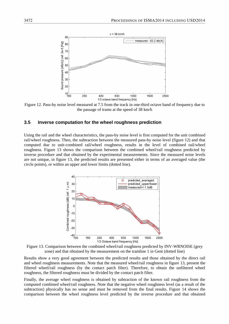
Figure 12. Pass-by noise level measured at 7.5 from the track in one-third octave band of frequency due to

the passage of trams at the speed of 38 km/h

3.5 Inverse computation for the wheel roughness prediction

Using the rail and the wheel characteristics, the pass-by noise level is first computed for the unit combined

rail/wheel roughness. Then, the subtraction between the measured pass-by noise level (figure 12) and that

computed due to unit-combined rail/wheel roughness, results in the level of combined rail/wheel

roughness. Figure 13 shows the comparison between the combined wheel/rail roughness predicted by

inverse procedure and that obtained by the experimental measurements. Since the measured noise levels

are not unique, in figure 13, the predicted results are presented either in terms of an averaged value (the

circle points), or within an upper and lower limits (dotted line).

Figure 13. Comparison between the combined wheel/rail roughness predicted by INV-WRNOISE (grey

zone) and that obtained by the measurement on the tramline 1 in Gent (dotted line)

Results show a very good agreement between the predicted results and those obtained by the direct rail

and wheel roughness measurements. Note that the measured wheel/rail roughness in figure 13, present the

filtered wheel/rail roughness (by the contact patch filter). Therefore, to obtain the unfiltered wheel

roughness, the filtered roughness must be divided by the contact patch filter.

Finally, the average wheel roughness is obtained by subtraction of the known rail roughness from the

computed combined wheel/rail roughness. Note that the negative wheel roughness level (as a result of the

subtraction) physically has no sense and must be removed from the final results. Figure 14 shows the

comparison between the wheel roughness level predicted by the inverse procedure and that obtained


directly by measurements on the wheels in the workshop. Results show a reasonable agreement at

frequencies higher than 400 Hz. At 250, 315 and 500 Hz, the wheel roughness became negative, the

reason why no value is shown at these frequencies.

Figure 14. Comparison between the wheel roughness level in one third octave band of frequency

predicted by INV-WRNOISE for a speed of 38 km/h and those obtained by measurements on the wheels

Performing a similar procedure for the measured results at different tram speeds e.g. 36, 38, 42 km/h, the

wheel roughness is presented as an averaged value. Figure 15 shows the predicted average wheel

roughness compared with the wheel roughness measured on 4 wheels in the workshop.

Figure 15. Comparison between the wheel roughness predicted by INV-WRNOISE and the average wheel

roughness measured on 4 wheels

At wavelengths smaller than 3 cm, the results show a better agreement with the measured value than those

at larger wavelength. This may be explained by the fact that the proposed inverse procedure is based on

the subtraction of the measured rail roughness from the predicted combined wheel/rail roughness. When

the combined wheel/rail roughness is dominated by the rail roughness, (here for the wavelength longer

than 3 cm) the subtraction tends to unreliable values. In this case, even a small error in the determination

of the combined wheel/rail roughness can produce a significant error in prediction of the wheel roughness.

Since the level of the rail roughness is much higher than the level of the wheel roughness, the rolling noise

is dominated by the rail roughness.


4 Conclusions

In the frame of the QUIET-TRACK project, an inverse computation technique was developed to evaluate

the wheel roughness using the measured sound pressure at receivers along an array of microphones beside

the tracks. The track-vehicle interaction parameters such as the rail and the wheel receptances, the track

decay rate (TDR), and the rail roughness are the other parameters needed for the inverse computation.

The wheel roughness prediction model was experimentally validated. A measurement campaign was

performed in Gent (BE) where the pass-by noise level for passage of Hermelijn trams at various speeds

were measured. A very good agreement was found between the combined wheel/rail roughness calculated

by INV-WRNOISE software and that obtained by the experimental measurements.

These results reveal the limitations of the application of the proposed inverse method. The prediction

model is applicable when the wheel roughness is no more than 5 dB lower than the rail roughness. This is

likely the case for passenger trains equipped with disc brakes. For freight trains with cast-iron block

brakes, the rolling noise is generally dominated by the wheel roughness, [9].Obviously, when the wheel

roughness is negligible in comparison to the rail roughness, the pass-by noise is not influenced by the

wheel roughness, and it is impossible to determine the wheel roughness based on pass-by noise

measurements. In that case however, a measurement of the rail roughness alone is sufficient to calculate

the rolling noise levels.

Acknowledgements

The results presented in this paper have been obtained within the frame of FP7 European QUIET-TRACK

project entitled: “Quiet Tracks for Sustainable Railway Infrastructures”. The financial support of the

European Commission is gratefully acknowledged.

References

[1] P.J. Remington, Wheel/rail rolling noise, I: Theoretical analysis, Journal of the Acoustical Society of

America 81, 1805-1823 (1987).

[2] D. Thompson, Railway Noise and Vibration: mechanism, modeling and means, ELSEVIER, (2009).

[3] G. Lombaert, G. Degrande, J. Kogut, and S. François, The experimental validation of a numerical

model for the prediction of railway induced vibrations, Journal of Sound and Vibration 297, (2006).

[4] F.L. Courtois, J.H. Thomas, F. Poisson, and J.-C. Pascal, Identification of the rail radiation using

beamforming and a 2D array, Proceeding of the conference Acoustics 2012, April (2012), France.

[5] D.A. Bies, C.H. Hansen, Engineering noise control: Theory and practice, Taylor & Francis (2009).

[6] D.J. Thompson and C.J.C. Jones, Sound radiation from a vibrating railway wheel. Journal of Sound

and Vibration, 253, (2), 401-419 (2002).

[7] X. Zhang, The directivity of railway noise at different speeds, Journal of sound and vibration, 329,

5273-5288 (2010).

[8] Tom Vanhonacker. Accurate quantification and follow up of rail corrugation on several rail transit

networks . proceedings of Railway Engineering Conference. London. (2007).

[9] A. Bracciali, and M. Pippert, and S. Cervello, Railway Noise: The Contribution of Wheels, Basics,

the Legal Frame. Lucchini, (2009).


simulation of railway rolling noise emission:...

Documents