simulation of ship motions Œ coupled heave, pitch...

Centre for Oil and Gas Engineering Center for Marine Science and Technology

Technical Report

Simulation of Ship Motions � Coupled Heave, Pitch and Roll

By Sheming Fan and Jinzhu Xia

20 March, 2002

woodsan

Centre for Marine Science & Technology, Technical Report # 2002-35 CMST Project # 366

Simulation of Ship Motions

2

SUMMARY

The time-domain strip theory for vertical and rolling motions has been extended to predict the coupling of heave, pitch and roll motions by combining hydrostatic restoring force and moments in heave, pitch and roll displacements. Corresponding computer program is developed. Time-domain simulations are performed for a Panamax Container ship at different headings and encounter frequencies. The coupling effect and parametric resonance are investigated. It is seen that parametric instability occurs when the ship sails in quartering waves and very low encounter frequency. In other computational wave conditions, the effects of coupling of heave, pitch and roll are small.


3

CONTENTS

1. INTRODUCTION 4

2. TIME-DOMAIN STRIP THEORY FORMULATION 4

3. CURRENT ASSUMPTIONS 6

4. NON-LINEAR TIME-DOMAIN HYDROELASTIC VERTICAL MOTIONS 6

5. NON-LINEAR TIME-DOMAIN ROLL MOTION 9

6. NUMERICAL METHODS 10

7. CALCULATIONS FOR A PANAMAX CONTAINER SHIP 11

8. CONCLUDING REMARKS 12

ACKNOWLEDGEMENTS 12

REFERENCES 13

FIGURES 14

APPENDIX 23


4

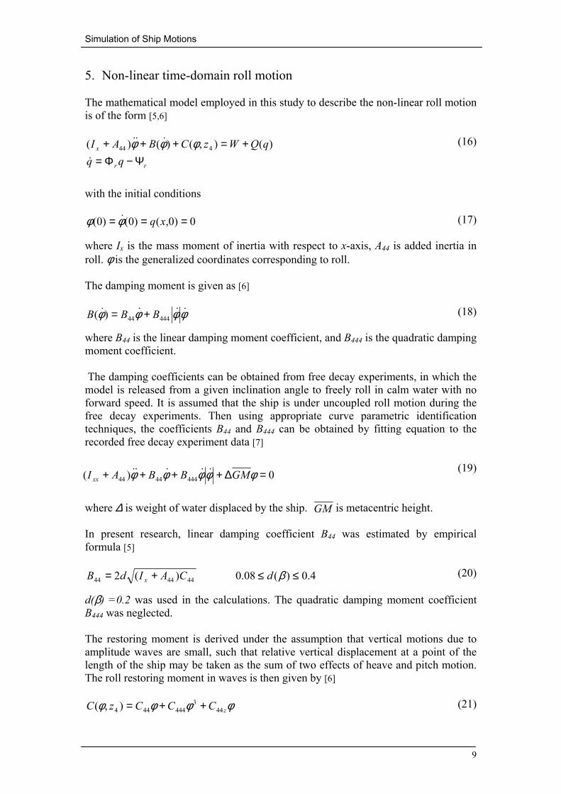
1. Introduction The coupling motions of heave, pitch and roll have been discovered from both experimental observations and theoretical simulations. An extreme phenomenon is parametric resonance. In this case, the energy in heave and pitch motions may be transferred to roll motion mode through non-linear coupling, which leads to excessive resonant rolling and stability problems [1]. Excessive roll motion increases the probability of seasickness of the crew, reduces the operability of the onboard systems and, in the worst case, cause capsize of the vessel. Because of the lateral symmetry of ship hull forms, linear theories are unable to account for the coupling between heave, pitch and roll. It is quite often that roll motion is treated as a single degree-of-freedom (DOF) dynamic problem, whereas heave and pitch are solved in a coupled two DOF system. Some previous studies have employed simplified hydrodynamic models to simulate this problem. Hydrodynamic memory effect due to the free-surface wave motion is not incorporated, which give significant uncertainties in the simulations. In other studies, the memory effect is expressed by a time convolution. The computation of time convolution limits the practical applications, and it is difficult to extend the theory to account for non-linear memory effects. A rational non-linear time-domain hydroelastic strip theory was developed in [2] to predict vertical wave loads and ship responses. It was extended to compute anti-symmetric wave-induced ship response [3]. Both studies modeled the hydrodynamic memory effect by a higher-order differential approximation instead of time-consuming numerical integration. Hence the computational efficiency is maintained while the complicated non-linear phenomenon is investigated. In the present research, the studies in [2] and [3] are merged to treat the coupling of roll motion with the vertical modes (heave and pitch) introduced by hydrostatic restoring forces and moments in heave, pitch and roll displacements. The coupled hydrostatic coefficients will be determined based on the instantaneous submerged area of each cross section and the integration over the ship length. Time-domain simulations are performed for a Panamax Container ship at different headings and encounter frequencies. 2. Time-domain strip theory formulation [2, 3] The Cartesian coordinate system (Figure 1) is defined as an �equilibrium� set of axes translating with mean forward speed U of the ship in the +x-direction. The origin is at the stern. The z=0 plane corresponds to the calm water level, and z is positive upwards. The x-z plane is coincident with the plane of the ship hull. The relative displacement between a ship section and wave surface can be expressed as


5

(1)

where l=2 and 3 denote the lateral and vertical movements; l=4 denotes the rotation about the x-axis. wl(x,t) is the displacement component of ship section and ξl(x,t) is the average displacement component of the wave at the ship section and is related to wave elevation with the Smith correction. The time-domain sectional hydrodynamic force vector F(x,t) consisting of the lateral, vertical and rotational components without convolution may be expressed by [2, 3]

(2)

where I(x,t) represents both the impulsive and memory vectors in the hydrodynamic

momentum; D/Dt is the total derivative with respect to time t, with U

being the forward speed of the ship; ; Aj(x)and Bj(x) are the so-called

frequency-independent hydrodynamic coefficient matrices derived by a rational

approximation from the frequency dependent added mass m(x,ω) and damping

coefficient N(x,ω)

(3)

where i is the imaginary unit and ω is the wave frequency. Equation 2 can be extended empirically to include the non-linear loading effects due to the time variation of the wetted ship surface by assuming that the coefficients Aj(x) and Bj(x) vary with not only the longitudinal position but also the instantaneous submergence. By integrating the higher-order differential equation in Equation 2, the sectional hydrodynamic force vector F(x,t) can be rewritten as

(4)

where m(x,z2,z3,z4) is the added mass matrix of the ship section when the oscillating frequency tends to infinity; DqJ/Dt accounts for the hydrodynamic memory effect governed by the following set of differential equations

4,3,2),(),(),( =−= ltxtxwtxz lll ξ

0)(

),(

0

)1( =−

=

∑=

+J

j

jjj Dt

DDtDtx

zAIB

IF

4,3,2,)(

)(

0,

0

1,

=−

−=−∑

∑

=

=

+

lkiB

iANmi J

j

jklj

J

j

jklj

klkl

ω

ωω

)(x

UtDt

D∂∂−

∂∂=

j

jj

t∂∂=)()(

DtD

DtD

DtD

xU

DtDtx Jqz

zmzmzmF −

∂∂−

∂∂+−= 2

2

2

)(),(


6

(5) The third term of F(x,t) in Equation 4 provides the momentum slamming force. It vanishes in the linear problem. According to physical judgements, this term is usually only taken into account when the ship section enters into the water. 3. Current assumptions There are some basic assumptions for the present problem as follows (1) Neglect the effect of horizontal motions � surge, sway and yaw. (2) Neglect hydroelastic effect on roll motion. (3) Neglect the effect of the variation of wetted surface on rolling added mass and

damping. (4) Neglect the hydrodynamic coupling between roll and vertical motions. Coupling

of roll motion with the vertical modes is introduced by hydrostatic restoring force and moments in heave, roll and pitch displacements.

Under the above assumptions, the hydrodynamics of the vertical and rolling motions can be treated separately. The motions will then be coupled through hydrostatic forces. 4. Non-linear time-domain hydroelastic vertical motions [2] By incorporation of the hydrostatic action and rolling effect in Equation 4, the total vertical non-linear external fluid force acting on a ship section can be expressed as

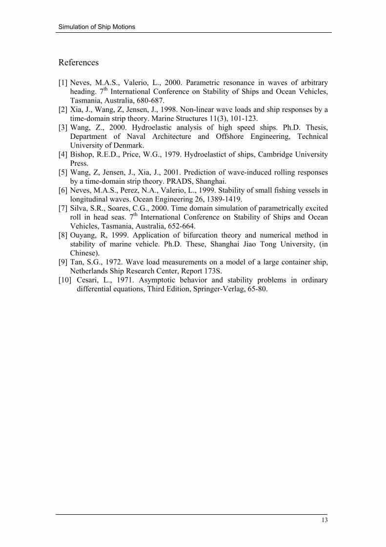
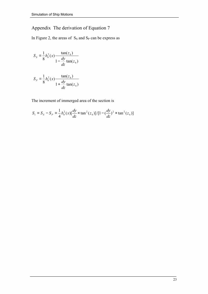
(6) where ρ is the density of the water and g is the gravitational acceleration. S0 denotes the instantaneous immersed area of the ship section due to vertical motions. S1 represents the increment of submerged area arising in rolling motions (Figure 2 and Appendix). For wall-sided hull forms this term will disappear, but for ships with flare, it may be significant

(7)

where b0(x) is the breadth at the calm water line, dy/dz represents the section flare slope at the calm water line, and z4 is the relative displacement between rolling motion and average wave slop across the section.

0

,...,2,1)(

0

1111

=

=+−−=∂

∂−−−−

q

zmBAqBqq

JjDtD

t jjJjjj

)()(),( 10233

23

2

SSgDt

DqDt

Dzzm

DtDz

xmU

DtzD

mtxZ J ++−∂∂−

∂∂+−= ρ

)](tan)(1/[)](tan)[(41)( 4

224

2201 z

dzdyz

dzdyxbxS ×−×=


7

The hull is modelled as a linear elastic non-uniform Timoshenko beam. The assumption of small rigid-body motions and structural distortions allows model superposition of the displacement [2, 4]

(8)

where wr is the rth unit dry mode shape, and pr the rth generalized principal coordinate of motion. In this analysis only the vertical response problem is consider. Therefore r=0 and 1 corresponds to heave and pitch motions, while r=2,3,�,n represents elastic distortions of the hull girder. The equation of motions for the ship hull can be written as

(9)

Hereafter overdot denotes differentiation with respect to time. In this equation, Z(x,t) is the total fluid action as represented by Equation 6, µ(x) the longitudinal distribution of mass of the ship structure, L the ship length, and asr, bsr, csr are the components of the generalized structural mass, damping and stiffness matrices

(10)

where δsr is the Kronecker delta function, Iy the longitudinal distribution of moment of inertia of the structure, θr the rth mode angular function of the ship hull girder beam in the x-z plane induced by vertical bending, αr the rth mode logarithmic damping decrement of the structure in vacuum, and ωr the rth mode eigenfrequency of the dry hull. In order to preserve the orthogonality between the rigid-body modes (heave and pitch), it is necessary that the mode shape w1(x) and x-axis intersect at the centre of mass of beam. It is assumed that the cross damping coefficients bsr (r≠s) can be neglected. By substituting Equation 6 into Equation 9, the equations of the fluid structure interaction can be obtained as

(11)

with the initial conditions

(12)

In the above equation, p is the generalized coordinate voter, p={p0,p1,�,pn}T, q is a voter used in the integration of the higher-order hydrodynamic equation, q={q0,q1,�,qJ}T; A,B,C are the generalized fluid added mass, damping and restoring

∑=

=n

rrr tpxwtxw

0)()(),(

.,...,1,0,)),(()]()()([0

nsdxwgtxZtpctpbtpaL s

n

rrsrrsrrsr =−=++ ∫∑

=

µ&&&

2

/

)(

rsrsrsr

rrsrsrsr

L srysrsrsr

ac

ab

dxIwwa

ωδπαωδ

θθµδ

=

=

+= ∫

ΨΦqqqQPWRpCcpBbpAa

+=+++=+++++

),(),()()()()()()()(

txtxttt

&

&&&

0)0,()0()0( === xqpp &


8

force coefficients, which are functions of t and p in the non-linear problem, R(t;p) represents the generalized combined action of the instantaneous hydrostatic restoring force and the structural gravitational force, W(t;p) is the generalized non-linear wave diffraction force, is the generalized �momentum slamming� force; Q(q) is the generalize �memorial� hydrodynamic force

(13)

In the above equations, prime indicates differentiation with respect to x. V is the relative vertical velocity between the section and the wave surface. The matrices Φ and Ψ in Equation 11 are, respectively, expressed by

(14)

(15)

−−

−−

=

−

−

1

2

1

0

100010

001000

);,(

J

J

BB

BB

tx

L

L

M

L

L

pΦ

+−

+−+−

=

−−

0)(

)()(

),;,(

22

11

00

VmBA

VmBAVmBA

tx

JJ

M&ppΨ

.,...,2,1,0,

|)()(

00

0),;,(

),;(

|)()]()([);(

])([);(

|);(

|)();(

);(

0'

2

3

0'

10

0'2''2

0''

nsr

wUqdxwUqwqQ

V

VVzm

txf

dxwftP

UUmwdxUUmwUmwtW

dxwSSgtR

wmwUdxwmwUtC

wUmwdxwwwwmUtB

dxwmwtA

LsJL sJsJs

m

L sms

LsL sss

L ss

LsrL srsr

LsrL rssrsr

L srsr

=

++−=

≥

<∂∂

=

=

′−−′−+′−=

−+=

+−=

−−−=

=

∫

∫∫∫∫∫

∫

&

&

&

&&&&&&

q

pp

pp

p

p

p

p

p

ξξξξξξ

µρ

),;( ppP &t


9

5. Non-linear time-domain roll motion The mathematical model employed in this study to describe the non-linear roll motion is of the form [5,6]

(16)

with the initial conditions

(17)

where Ix is the mass moment of inertia with respect to x-axis, A44 is added inertia in roll. φ is the generalized coordinates corresponding to roll. The damping moment is given as [6]

(18)

where B44 is the linear damping moment coefficient, and B444 is the quadratic damping moment coefficient. The damping coefficients can be obtained from free decay experiments, in which the model is released from a given inclination angle to freely roll in calm water with no forward speed. It is assumed that the ship is under uncoupled roll motion during the free decay experiments. Then using appropriate curve parametric identification techniques, the coefficients B44 and B444 can be obtained by fitting equation to the recorded free decay experiment data [7]

(19)

where ∆ is weight of water displaced by the ship. is metacentric height. In present research, linear damping coefficient B44 was estimated by empirical formula [5]

(20)

d(β) =0.2 was used in the calculations. The quadratic damping moment coefficient B444 was neglected. The restoring moment is derived under the assumption that vertical motions due to amplitude waves are small, such that relative vertical displacement at a point of the length of the ship may be taken as the sum of two effects of heave and pitch motion. The roll restoring moment in waves is then given by [6]

(21)

rr

x

qqqQWzCBAI

Ψ−Φ=+=+++

&

&&& )(),()()( 444 φφφ

0)0,()0()0( === xqφφ &

0)( 4444444 =∆++++ φφφφφ GMBBAI xx&&&&&

φφφφ &&&&44444)( BBB +=

φφφφ zCCCzC 443

444444 ),( ++=

4.0)(08.0)(2 444444 ≤≤+= βdCAIdB x

GM


10

where C44 and C444 represent linear and third order roll restoring coefficient [5]

(22)

where zb is vertical position of buoyancy centre of the section. C444 can be obtained from the hydrostatic curve of the ship [8]. It is neglected in present calculations. C44z represent time-dependent variation of hull restoring characteristic due to heave motion of a section (Figure 3), to second order [6],

(23)

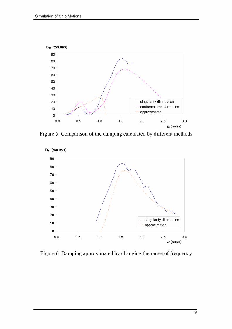
where the definition of b0(x) and dy/dz are the same as in Equation 7. zg is vertical coordinate of ship centre of gravity, z3 is the relative vertical displacement between a ship section and the wave surface. In equation 17, q(x,t) is a variation used in the integration of the higher-order hydrodynamic equation; W(t) is the generalized wave force and Q(q) is the generalized hydrodynamic �memory� force. 6. Numerical methods [2, 3] The second-order central difference scheme is used to determine the eigenvalues and principal modes of the free-free non-uniform Timoshenko beam. The modes of displacement wr, bending slope, shearing angle, bending moment Mr, shearing force Vr and the natural frequencies ω can be simultaneously obtained through an iterative procedure with very small computational effort. A multi-parameter conformal transformation technique is used to solve the vertical two-dimensional frequency-domain hydrodynamic coefficients (added mass and added damping) of the sections at several draughts. The singularity distribution method is used to determine the two-dimensional frequency-domain hydrodynamic coefficients for roll motion. Equation 3 is exactly satisfied at 2J-1 frequencies. In order to achieve the best approximation within a given frequency range, the frequency-independent hydrodynamic coefficients Aj and Bj are obtained by minimizing

(24)

with

(25)

∫ −−=L gz dxzxbz

dzdyxbgC 30

2044 )]()(

21[ρ

GMdxzSzxb

gCL gb ∆≈−+= ∫ ])

12)(

([20

44 µρ

{ }∑=

+K

rrr

1

22 )Im()Re( εε

4,3])([)(0

,, =−+=∑=

kBiN

mAiJ

jkj

r

kkkj

jrr ω

ωε


11

where ωr are discrete circular frequencies within the given ship-dependent frequency range. From numerical tests it is found that, in order to reach good agreement between the original and the approximated frequency-domain hydrodynamic coefficients, a third-order differential approach (J=3) is necessary and sufficient for most sectional shapes except for roll of the extreme U-shaped sections (Figure 4). In this case, the twin peak appears in the frequency response of damping (Figure 5). It is difficult to approximate correctly for the whole frequency range by third-order (or even higher-order) differential approach. In order to get a more reasonable approximation, added damping was only approximated in higher frequency range because the damping in low frequency is much smaller than that in high frequency (Figure 6). The non-linear differential equations for the coupled fluid-structure system are integrated in the time domain by using the Adams predictor-corrector scheme. The fourth-order Runge-Kutta method is used to predict the function values at the previous four time steps. 7. Calculations for a Panamax Container Ship Time-domain simulations are performed for a Panamax Container Ship. A detailed description of the experiments including the body plan and the main particulars of the ship can be found in Tan [9]. The uncoupled results have been compared with model tests. The agreement is acceptable for the linear roll motion and non-linear vertical modes [3,5]. Considering the harmonic character of time varying terms, the equations 11 and 17 are recognized as forming a set of coupled Mathieu equations. This type of system of ordinary differential equations with periodic coefficients may be, in general, subjected to parametric resonance for encounter frequencies close to [10]

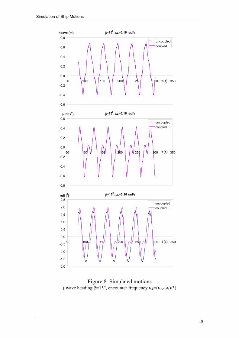
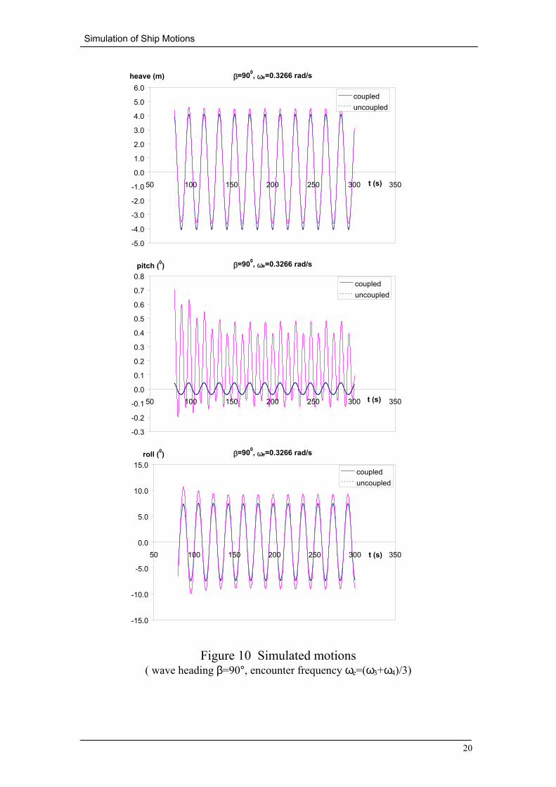
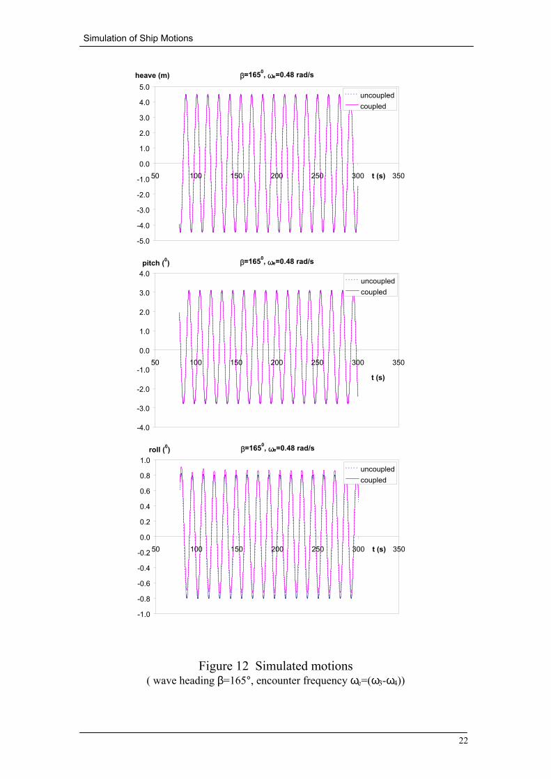
(26) For the Panamax Container Ship, the nature frequencies of heave, roll and pitch are ω3=0.73 rad/s, ω4=0.25 rad/s, and ω5=0.73rad/s, respectively. Following the above analyses, the simulations are conducted for three wave headings: β=15, 90, 165 degrees (180 degrees denote head waves). For each wave heading, two encounter frequencies, which probably lead to parametric resonance, are considered. The range of wavelength to ship length ratio is: λ/L=0.5∼ 2.5. The wave amplitude was kept constant at 5 m. Ship speed is 24.5 knot. The computational results are showed in Figure 7 to 12. For each time series, uncoupled results are also given. Figure 7 and 8 give the results for wave heading β=15° and encounter frequencies ωe=0.12 rad/s (4ωe=ω3-ω4) and ωe=0.16 rad/s (3ωe=ω3-ω4). In Figure 7, amplitudes of uncoupled roll responses are of the order of 4 degrees; the roll response from the coupled set of equations is of the order of 13 degrees. Much large coupled roll motions are found in this condition. Coupled heave and pitch are also very different

5,4,3,,...,2,1,2,,m e ==±= jimor iji ωωωω


12

from the uncoupled solution, but these motions are small in amplitudes. In Figure 8, coupled roll motion is not very different from uncoupled motions. Coupled heave and pitch motions are nearly the same as uncoupled motions. Figure 9 and 10 present the results from the beam waves. The encounter frequencies are ωe=0.49 rad/s (2ωe=ω3+ω4) and ωe=0.3266 rad/s (3ωe=ω3+ω4). In this case, coupled pitch motions change a lot. The effects of coupled motions are bigger in lower frequency than that in higher frequency. Both coupled and uncoupled pitch motions are small in amplitude. Coupled heave and roll motions are not very different form uncoupled motions. Figure 11 and 12 show the results for the bow waves (wave heading β=165°). The encounter frequencies are ωe=0.98 rad/s (ωe=ω3+ω4) and ωe=0.48 rad/s (ωe=ω3-ω4). The coupled heave and pitch motions are nearly the same as uncoupled motions. The mean values of coupled roll motions are biased. It may be due to the bias of pitch motions. Both coupled and uncoupled roll motions are small. It is seen from these comparisons that parametric instability occurs when the ship sails in quartering waves and very low encounter frequency. In other computational wave conditions, the effects of coupling of heave, pitch and roll are small. 8. Concluding remarks The time-domain strip theory for vertical and rolling motions has been extended to predict the coupling of heave, pitch and roll motions by combining hydrostatic restoring force and moments in heave, pitch and roll displacements. Corresponding computer program has been developed. Time-domain simulations were performed for a Panamax Container ship at different headings and encounter frequencies. The coupling effect and parametric resonance were investigated. Acknowledgements The authors would like to thank Dr Zhaohui Wang of the Clough Engineering Ltd for providing her computer program on roll motion simulation and for valuable discussions and help in the course of this work. Thanks also go to Dr Martin Renilson, now with Qinetiq, UK, for valuable discussions. The authors are grateful for the financial support under a UWA Small Grant awarded to J. Xia and a Centre of Excellence funding allocated to the Centre for Marine Science and Technology by the Western Australia state government.


13

References [1] Neves, M.A.S., Valerio, L., 2000. Parametric resonance in waves of arbitrary

heading. 7th International Conference on Stability of Ships and Ocean Vehicles, Tasmania, Australia, 680-687.

[2] Xia, J., Wang, Z, Jensen, J., 1998. Non-linear wave loads and ship responses by a time-domain strip theory. Marine Structures 11(3), 101-123.

[3] Wang, Z., 2000. Hydroelastic analysis of high speed ships. Ph.D. Thesis, Department of Naval Architecture and Offshore Engineering, Technical University of Denmark.

[4] Bishop, R.E.D., Price, W.G., 1979. Hydroelastict of ships, Cambridge University Press.

[5] Wang, Z, Jensen, J., Xia, J., 2001. Prediction of wave-induced rolling responses by a time-domain strip theory. PRADS, Shanghai.

[6] Neves, M.A.S., Perez, N.A., Valerio, L., 1999. Stability of small fishing vessels in longitudinal waves. Ocean Engineering 26, 1389-1419.

[7] Silva, S.R., Soares, C.G., 2000. Time domain simulation of parametrically excited roll in head seas. 7th International Conference on Stability of Ships and Ocean Vehicles, Tasmania, Australia, 652-664.

[8] Ouyang, R, 1999. Application of bifurcation theory and numerical method in stability of marine vehicle. Ph.D. These, Shanghai Jiao Tong University, (in Chinese).

[9] Tan, S.G., 1972. Wave load measurements on a model of a large container ship, Netherlands Ship Research Center, Report 173S.

[10] Cesari, L., 1971. Asymptotic behavior and stability problems in ordinary differential equations, Third Edition, Springer-Verlag, 65-80.


14

z y U calm water level o x

Figure 1 Equilibrium coordinate system Ss z4 Sp b0(x) dz dy

Figure 2 Effect of roll on heave for a unit section Increment of vertical restoring force ∆Z=ρg(Ss-Sp)


15

z3 b0(x) dz dy

Figure 3 Variation of sectional beam with relative vertical displacement

Roll hydrostatic moment coefficient changes with the change of inertia, area centre and submerged volume

Figure 4 Section plan of #10 station


16

Figure 5 Comparison of the damping calculated by different methods

Figure 6 Damping approximated by changing the range of frequency

0

10

20

30

40

50

60

70

80

90

0.0 0.5 1.0 1.5 2.0 2.5 3.0ω (rad/s)

B44 (ton.m/s)

singularity distributionconformal transformationapproximated

0

10

20

30

40

50

60

70

80

90

0.0 0.5 1.0 1.5 2.0 2.5 3.0ω (rad/s)

B44 (ton.m/s)

singularity distributionapproximated


17

Figure 7 Simulated motions ( wave heading β=15°, encounter frequency ωe=(ω3-ω4)/4)

β=150, ωe=0.12 rad/s

-0.6

-0.4

-0.2

0.0

0.2

0.4

0.6

0.8

1.0

1.2

50 100 150 200 250 300 350t (s)

heave (m)

uncoupledcoupled

β=150, ωe=0.12 rad/s

-0.8

-0.6

-0.4

-0.2

0.0

0.2

0.4

0.6

0.8

50 100 150 200 250 300 350t (s)

pitch (0)

uncoupledcoupled

β=150, ωe=0.12 rad/s

-10.0

-5.0

0.0

5.0

10.0

15.0

50 100 150 200 250 300 350t (s)

roll (0)

uncoupledcoupled


18

Figure 8 Simulated motions ( wave heading β=15°, encounter frequency ωe=(ω3-ω4)/3)

β=150, ωe=0.16 rad/s

-0.6

-0.4

-0.2

0.0

0.2

0.4

0.6

0.8

50 100 150 200 250 300 350t (s)

heave (m)

uncoupledcoupled

β=150, ωe=0.16 rad/s

-0.8

-0.6

-0.4

-0.2

0.0

0.2

0.4

0.6

50 100 150 200 250 300 350t (s)

pitch (0)

uncoupledcoupled

β=150, ωe=0.16 rad/s

-2.0

-1.5

-1.0

-0.5

0.0

0.5

1.0

1.5

2.0

2.5

50 100 150 200 250 300 350t (s)

roll (0)

uncoupledcoupled


19

Figure 9 Simulated motions ( wave heading β=90°, encounter frequency ωe=(ω3+ω4)/2)

β=900, ωe=0.49 rad/s

-6.0

-4.0

-2.0

0.0

2.0

4.0

6.0

50 100 150 200 250 300 350t (s)

heave (m)

coupleduncoupled

β=900, ωe=0.49 rad/s

-0.3

-0.2

-0.1

0.0

0.1

0.2

0.3

0.4

0.5

0.6

50 100 150 200 250 300 350t (s)

pitch (0)

coupleduncoupled

β=900, ωe=0.49 rad/s

-6.0

-4.0

-2.0

0.0

2.0

4.0

6.0

50 100 150 200 250 300 350t (s)

roll (0)

coupleduncoupled


20

Figure 10 Simulated motions ( wave heading β=90°, encounter frequency ωe=(ω3+ω4)/3)

β=900, ωe=0.3266 rad/s

-5.0

-4.0

-3.0

-2.0

-1.0

0.0

1.0

2.0

3.0

4.0

5.0

6.0

50 100 150 200 250 300 350t (s)

heave (m)

coupleduncoupled

β=900, ωe=0.3266 rad/s

-0.3

-0.2

-0.1

0.0

0.1

0.2

0.3

0.4

0.5

0.6

0.7

0.8

50 100 150 200 250 300 350t (s)

pitch (0)

coupleduncoupled

β=900, ωe=0.3266 rad/s

-15.0

-10.0

-5.0

0.0

5.0

10.0

15.0

50 100 150 200 250 300 350t (s)

roll (0)

coupleduncoupled


21

Figure 11 Simulated motions

( wave heading β=165°, encounter frequency ωe=(ω3+ω4))

β=1650, ωe=0.98 rad/s

-0.5

-0.4

-0.3

-0.2

-0.1

0.0

0.1

0.2

0.3

0.4

0.5

50 100 150 200 250t (s)

heave (m)

uncoupledcoupled

β=1650, ωe=0.98 rad/s

-0.8

-0.6

-0.4

-0.2

0.0

0.2

0.4

0.6

0.8

1.0

1.2

50 100 150 200 250t (s)

pitch (0)

uncoupledcoupled

β=1650, ωe=0.98 rad/s

-0.15

-0.10

-0.05

0.00

0.05

0.10

0.15

50 100 150 200 250t (s)

roll (0)

uncoupledcoupled


22

Figure 12 Simulated motions ( wave heading β=165°, encounter frequency ωe=(ω3-ω4))

β=1650, ωe=0.48 rad/s

-5.0

-4.0

-3.0

-2.0

-1.0

0.0

1.0

2.0

3.0

4.0

5.0

50 100 150 200 250 300 350t (s)

heave (m)

uncoupledcoupled

β=1650, ωe=0.48 rad/s

-4.0

-3.0

-2.0

-1.0

0.0

1.0

2.0

3.0

4.0

50 100 150 200 250 300 350

t (s)

pitch (0)

uncoupledcoupled

β=1650, ωe=0.48 rad/s

-1.0

-0.8

-0.6

-0.4

-0.2

0.0

0.2

0.4

0.6

0.8

1.0

50 100 150 200 250 300 350t (s)

roll (0)

uncoupledcoupled


23

Appendix The derivation of Equation 7 In Figure 2, the areas of SS and SP can be express as The increment of immerged area of the section is

)tan(1

)tan()(81

)tan(1

)tan()(81

4

420

4

420

zdzdy

zxbS

zdzdy

zxbS

P

S

+=

−=

)](tan)(1/[)](tan)[(41

422

422

01 zdzdyz

dzdyxbSSS PS ×−×=−=

simulation of ship motions Œ coupled heave, pitch...

Documents