simulation of subcritical flow pattern in 180° uniform and convergent … · 2016-12-01 ·...

Water Science and Engineering, 2011, 4(3): 270-283doi:10.3882/j.issn.1674-2370.2011.03.004 http://www.waterjournal.cn

e-mail: [email protected]

*Corresponding author (e-mail: [email protected]) Received Feb. 17, 2011; accepted Aug. 29, 2011

Simulation of subcritical flow pattern in 180 uniform and convergent open-channel bends using SSIIM 3-D model

Rasool GHOBADIAN*1, Kamran MOHAMMADI2

1. Department of Water Engineering, Razi University, Kermanshah 6715685438, Iran 2. Department of Water Engineering, University of Tabriz, Tabriz 5166616471, Iran

Abstract: In meandering rivers, the flow pattern is highly complex, with specific characteristics at bends that are not observed along straight paths. A numerical model can be effectively used to predict such flow fields. Since river bends are not uniform–some are divergent and others convergent–in this study, after the SSIIM 3-D model was calibrated using the result of measurements along a uniform 180° bend with a width of 0.6 m, a similar but convergent 180° bend, 0.6 m to 0.45 m wide, was simulated using the SSIIM 3-D numerical model. Flow characteristics of the convergent 180° bend, including lengthwise and vertical velocity profiles, primary and secondary flows, lengthwise and widthwise slopes of the water surface, and the helical flow strength, were compared with those of the uniform 180° bend. The verification results of the model show that the numerical model can effectively simulate the flow field in the uniform bend. In addition, this research indicates that, in a convergent channel, the maximum velocity path at a plane near the water surface crosses the channel’s centerline at about a 30° to 40° cross-section, while in the uniform bend, this occurs at about the 50° cross-section. The varying range of the water surface elevation is wider in the convergent channel than in the uniform one, and the strength of the helical flow is generally greater in the uniform channel than in the convergent one. Also, unlike the uniform bend, the convergent bend exhibits no rotational cell against the main direction of secondary flow rotation at the 135° cross-section. Key words: flow pattern; numerical simulation; convergent 180° bend; SSIIM 3-D model

1 Introduction Predicting river behavior at bends is important since rivers rarely run on straight paths in

nature, and most rivers have meandering forms. For meandering rivers, flow patterns are very complex with specific characteristics at bends. In general, factors influencing flow at a bend include the centrifugal force due to flow curvature and non-uniformity of vertical velocity profiles, the cross-sectional stress, and the pressure gradient in the radial direction caused by the lateral slope of the water surface (Chow 1959). Synchronous effects of such factors create a flow called helical flow.

Many studies have been performed to investigate flow characteristics and patterns in 180° bends with solid beds, of which Mockmore (1944) is the earliest. Mockmore’s research was

Rasool GHOBADIAN et al. Water Science and Engineering, Sep. 2011, Vol. 4, No. 3, 270-283 271

substantially criticized because of setting the radial velocity component at zero (Mansuri 2006). Rozovskii (1957) was among the first researchers who performed comprehensive studies in this field. The most important result Rozovskii obtained was the three-dimensional distribution of the flow field, and the research also showed the velocity component in the radial direction. Mosonyi and Gotz (1973) were the first who paid attention to the distribution of helical flow strength and its changes along channels. Their research showed that the secondary flow can be well described by its strength changes. For the first time, they reported the presence of the second cycle of the secondary flow near the internal bend, which only occurs at < 10B H (B is the bed width, and H is the water depth). Leschziner and Rodi (1979) presented their three-dimensional numerical model using the finite difference method. The most important result these researchers reported was the effect of the lengthwise pressure gradient on the flow pattern in swift bends. Lien et al. (1999) investigated the effect of secondary flow on depth-averaged equations using a stress diffusion matrix and studied the flow pattern at a 180° bend with a rigid bed using a two-dimensional numerical model. The research indicated the effect of secondary flow on the maximum velocity path along the channel. Booij (2003) modeled the structure of secondary flow at a 180° bend using the large eddy simulation method. The most important point of his research was that the -k turbulence model fails to model the rotation against the direction of secondary flow near the external wall. Olsen (2006) also did extensive research in this field in 2005. Mansuri (2006) studied the over-time bed evolution in 180° river bends with the SSIIM 3-D model. Ghobadian et al. (2010) also used the SSIIM 3-D numerical model to investigate flow characteristics in 180° divergent bends. In their research, several factors, including lengthwise and vertical velocity profiles, bed shear stress distributions, lengthwise and widthwise slopes of the water surface, and helical flow strength, were compared in 180° divergent and uniform bends.

Review of the research shows that most of the research has focused on 180° bends with uniform widths. This study simulated a flow field in a convergent 180° bend with the SSIIM 3-D numerical model and compared it with the results from a uniform 180° bend, so as to obtain a better understanding of flow patterns and characteristics in convergent channels.

2 Mathematical model and methods 2.1 Numerical methods

The SSIIM 3-D model is applied to some researches related to river engineering, environmental engineering, hydraulic research, and sedimentation research. Using non-dislocated non-orthogonal three-dimensional grids, this model solves Navier-Stokes equations and the

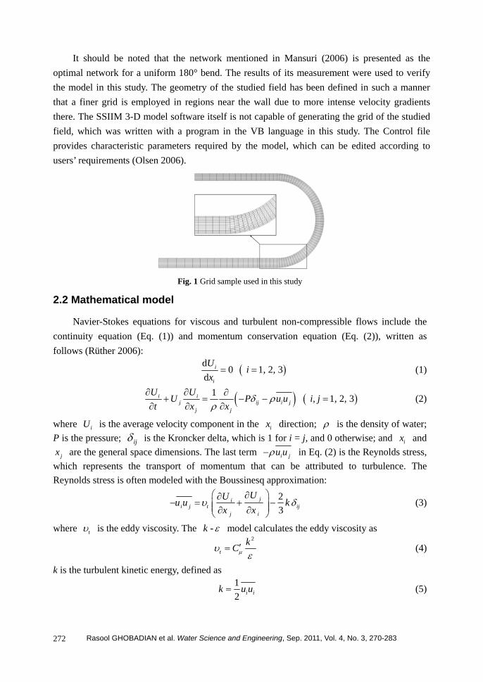
-k turbulence model. In this model, the control volume technique is used for discretization by means of the power law scheme or second-order upwind scheme (Olsen 2006). Model input data are given to software by specific files, of which the Control and Koordina files are commonly used. Geometric coordinates of the bed structured grid of studied bends are specified in the Koordina file. Fig. 1 shows the convergent 180° bend examined in this study, which has a grid size of 91 91 7, in the lengthwise, widthwise and vertical directions, respectively.


It should be noted that the network mentioned in Mansuri (2006) is presented as the optimal network for a uniform 180° bend. The results of its measurement were used to verify the model in this study. The geometry of the studied field has been defined in such a manner that a finer grid is employed in regions near the wall due to more intense velocity gradients there. The SSIIM 3-D model software itself is not capable of generating the grid of the studied field, which was written with a program in the VB language in this study. The Control file provides characteristic parameters required by the model, which can be edited according to users’ requirements (Olsen 2006).

Fig. 1 Grid sample used in this study

2.2 Mathematical model

Navier-Stokes equations for viscous and turbulent non-compressible flows include the continuity equation (Eq. (1)) and momentum conservation equation (Eq. (2)), written as follows (Rüther 2006):

d0 1, 2, 3

di

i

Ui

x (1)

1 1, 2, 3 i ij ij i j

j j

U UU P u u i, j

t x x (2)

where iU is the average velocity component in the ix direction; is the density of water; P is the pressure; ij is the Kroncker delta, which is 1 for i = j, and 0 otherwise; and ix and

jx are the general space dimensions. The last term i ju u in Eq. (2) is the Reynolds stress, which represents the transport of momentum that can be attributed to turbulence. The Reynolds stress is often modeled with the Boussinesq approximation:

23

jii j t ij

j i

UUu u kx x

(3)

where t is the eddy viscosity. The -k model calculates the eddy viscosity as 2

tkC (4)

k is the turbulent kinetic energy, defined as

12 i ik u u (5)


k is modeled as

tj k

j j k j

k k kU Pt x x x

(6)

where kP is given by

j j ik t

i i j

U U UPx x x

(7)

The dissipation of k is denoted by , and modeled as

2

1 2t

j kj j j

U C P Ct x x x k k

(8)

In Eqs. (4) through (8), C , k , , 1C , and 2C are empirical constants, which were determined experimentally to be 0.09, 1.0, 1.3, 1.44, and 1.92, respectively (Launder and Spalding 1974).

Boundary conditions for Navier-Stokes equations (e.g., boundary conditions for inflow, outflow, the water surface, and the bed/wall) are similar to those of the diffusion-convection equation. Dirichlet boundary conditions have to be given as the inflow boundary, which is relatively straightforward for velocity. Usually it is more difficult to specify the turbulence. To specify the eddy viscosity, it is possible to estimate the shear stress ( ) at the entrance bed using a given velocity. Then, the turbulent kinetic energy k at the entrance bed is determined by the following equation:

kC

(9)

With the eddy viscosity t and turbulent kinetic energy k at the bed, Eq. (4) gives the value of at the bed. If k is assumed to vary linearly from the bed to the surface, then Eq. (4), together with the profile of the eddy viscosity, can be used to calculate the vertical distribution of . A zero gradient condition was used for the outflow boundary.

The free surface is computed using a fixed-lid approach, with zero gradients for all variables. The location of the fixed lid and its movement as a function of time and the flow field are computed with the Bernoulli algorithm. The algorithm is based on the pressure field. It uses the Bernoulli equation along the water surface to compute the water surface location based on a fixed point downstream of the bend in this study.

The wall law for rough boundaries (Schlichting 1979) is used as a boundary condition for the bed/wall:

*s

1 30lnU ykU

(10)

where *U is the shear velocity, U is the velocity at the center of the grid cell closest to the bed, is a constant equal to 0.4, y is the distance from the wall to the center of the grid cell, and sk is the wall roughness.


3 Results and discussion3.1 Verification of 3-D numerical model

The studied field is a channel with a 180° bend used in Pirestani’s lab studies (Pirestani 2004). The bend has two straight paths, upstream and downstream, which were 7.2 m and 5.2 m long, respectively. Its wall and bed were made of plexiglas with a wall roughness of 0.000 1 m ( sk = 0.000 1 m). The flow pattern was studied at a flow rate of 30 L/s and a water depth of 0.15 m at the channel entrance, and, in order to verify numerical modeling, the results from modeling in the bend with a uniform 0.6 m width were compared with Pirestani’s lab results (Pirestani 2004), as shown in Figs. 2 through 4, where H is the water depth, h is the distance from the bed, B is the bed width, and b is the distance from the internal wall. It should be noted that in Pirestani’s research, flow velocities were measured at different depths at 91 cross-sections along the bend with a two-dimensional portable emissions measurement systems (PEMS).

Fig. 2 Comparison of vertical velocity profiles with Fig. 3 Comparison of lengthwise velocity profiles measured data at 180 cross-section at plane of h = 0.145 m with measured data

Fig. 4 Comparison of velocity profiles at plane near water surface (h = 0.145 m) at different cross-sections with measured data


To find the optimal grid size, grid independency investigations were performed. The grid size was changed from a coarse grid size of 71 12 7 in lengthwise, widthwise, and vertical directions, respectively, to the finest grid size of 351 35 15. Through comparison of maximum and minimum velocities, pressure, and turbulent kinetic energy in different grid cells, the grid size of 91 91 7 was finally selected as the optimal grid size. Power law and second-order upwind methods were used for discretization of the convectional term. The result showed no significant difference between the velocity profiles calculated by the two methods. Therefore, to continue, the power law method was used.

Figs. 2 through 4 indicate that velocity profiles calculated by numerical modeling are in complete agreement with lab-measured data. Statistical indicators (e.g., RMSE and ME ) were used to compare values of calculated and measured velocities at a plane of h = 0.145 m:

2RMS M P

1

1 N

i ii

E V VN

(11)

M M P1

1 N

i ii

E V VN

(12)

where RMSE is the root mean square error, ME is the mean error, N is the number of measured data, and MiV and PiV are the values of the ith measured and calculated velocities, respectively. Results of statistical comparison are presented in Table 1. The low values of

RMSE and ME in the table indicate that the numerical model effectively simulates the flow field in uniform bends.

Table 1 Statistical indicators of calculated and measured velocities at plane near water surface

Cross-section ( ) RMSE (m/s) ME (m/s)

10 0.074 –0.066

40 0.042 –0.009

90 0.048 0.018

130 0.043 0.015

170 0.042 0.012

3.2 Comparison of lengthwise velocity profiles in convergent and uniform bends

In this study, the results from a convergent channel bend with a width ranging from 0.6 m at the beginning of the bend to 0.45 m at the end of the bend were compared with those of a channel with a uniform 0.6 m width in order to compare flow characteristics of uniform channels with those of convergent ones. Fig. 5 shows the varying trends of lengthwise velocity profiles at the plane near the water surface for both uniform and convergent channels. The velocity profile of the convergent channel shows slower velocities at the 0° cross-section. This is due to the higher level of the water surface at the beginning of the bend of this channel, which will be discussed later.

At other cross-sections, velocity is faster in the convergent channel than in the uniform one because the channel is narrower, and there is an increase in flow rate per unit width. Also,


the lengthwise velocity profiles have the same shape in both channels, which shows that the maximum lengthwise velocity occurs near the internal wall at the beginning of the bend, and, after entering the bend, it migrates gradually toward the external wall.

Fig. 6 shows the path of maximum velocity at the plane near the water surface. As can be seen from this figure, the maximum velocity path cuts the centerline of the channel at about the 50° cross-section within the uniform bend while this occurs at about the 30º to 40º cross-section within the convergent channel. This indicates that, in the convergent bend, centrifugal force dominance over the flow field increases at a shorter distance from the beginning of the bend. In other words, the effect of the lengthwise pressure gradient dominates the effect of secondary flow strength at a shorter distance from the beginning of the convergent bend, so the maximum velocity migrates toward the external wall at a shorter distance from the beginning of the bend. Moreover, in both cases, maximum velocity path becomes a tangent to the bend external wall near the 100º cross-section and remains in this state until it reaches the end of the bend.

Fig. 5 Comparison of velocity profiles at plane near water surface (h = 0.145 m) for different cross-sections of uniform and convergent channels

Fig. 6 Comparison of maximum velocity paths at plane of h = 0.145 m for uniform and convergent channels


3.3 Comparison of vertical velocity profiles

Vertical velocity profiles were taken into account at three cross-sections: 0º, 45º, and 90º. As can be seen from Fig. 7, at the 0º cross-section, vertical velocity profiles show higher values in the uniform channel than in the convergent one due to the higher level of the water surface at the beginning of the convergent bend, which will be discussed in Section 3.5. Also, the maximum vertical velocity profile occurs at a distance of 0.25 m from the internal wall of the channel and velocities show low values at distances close to the walls. In addition, unlike that at the 0º cross-section, the vertical velocity is larger in the convergent channel than in the uniform one at the 90º cross-section. One of the reasons is that the decrease in cross-section width leads to the reduction of water depth. On the other hand, with a careful look at vertical velocity profiles, it can be seen that there is a high-speed flow core near the water surface and the internal wall at the 0º cross-section of the bend, but this core moved closer to the channel bed and external wall beyond the 90°cross-section. Also, values of velocity near the water surface in profiles shown in Fig. 7 show clearly the behavior of their velocity profiles at the plane near the water surface in Fig. 6.

Fig. 7 Comparison of vertical velocity profiles at different cross-sections of uniform and convergent channels (Unit of velocity is m/s)

3.4 Comparison of secondary flows and velocity distributions at different cross-sections

Figs. 8 and 9 illustrate the varying trends of secondary flow and velocity magnitude for 0°, 45°, 90°, 135°, and 180° cross-sections in the uniform and convergent bends. It can be seen that the distributions of velocity magnitude are almost identical for both channels, and that the maximum velocity migrates toward the external wall beyond the 90° cross-section. But, as expected, the velocity and its changes are larger in the convergent bend than in the uniform bend, because they are affected by narrowness. With a more careful look at velocity values, it is possible to explain the shapes and behaviors of vertical velocity profiles at different cross-sections in Fig. 7.

A rotational cell against the direction of secondary flow (a counter-rotating cell) is observed close to the internal wall near the water surface at the 135° cross-section in the


channel with a uniform bend (the oval part shown in Fig. 8(d)). In this region, within a small cell, widthwise velocity components run against the direction of water surface velocities between the internal wall and the centerline of the channel. Such a rotational cell, which runs against the direction of main secondary flow, was not observed at the 135° cross-section of the convergent channel. Other characteristics of secondary flows at different cross-sections of the two channels are almost identical. The core of secondary flow lies in the region between the centerline and internal wall of the bend at the 45° cross-section. It moves toward the centerline of the channel at about the 90° cross-section and remains in this area until the end of the bend.

Fig. 8 Velocity distributions and secondary flows at different cross-sections in uniform channel

Fig. 9 Velocity distributions and secondary flows at different cross-sections in convergent channel


3.5 Comparison of lengthwise and widthwise water surface slopes and helical flow strength

In both channels, the widthwise slope of the water surface forms before the flow reaches the bend (Fig. 10). This phenomenon is caused by the change of the lengthwise momentum direction due to flow entering the bend, which causes flow to be affected for a short interval before the bend entrance. Then, after the flow reaches the bend, the water surface changes at the external wall and internal wall due to the effect of the centrifugal force. For both channels, the water surface rises at the external wall before the 30° cross-section, and then it decreases. The widthwise elevation difference of the water surface reaches nearly zero at the end of bends in both cases.

Fig. 10 Varying trend of lengthwise water surface at internal and external walls of uniform and convergent channels (d is distance from beginning of channel, and h* is dimensionless water depth ratio)

The water surface varying trends are clearly different for the two channels. The range of water surface elevation changes is much wider in the convergent channel than in the uniform channel. Fluctuation changes can be observed on the water surface by careful looking at the flow pattern at the end of the uniform bend (the enlarged part in Fig. 10), which is caused by straightening of the bend path. This phenomenon was not observed at the exit of the convergent bend. It can be seen from Fig. 11 that the widthwise elevation difference of the water surface occurs before the beginning of the bend. Such an elevation difference increases after the flow enters the bend and decreases as the flow approaches the exit of the bend, reaching zero shortly after the flow exits the bend.

In general, the widthwise water surface elevation difference is larger in the convergent channel than in the uniform one due to the existence of larger centrifugal force. The maximum elevation difference occurs 13.1 m away from the beginning of the convergent bend (at about the 130° cross-section).

Helical flow strength was used to examine the trend of secondary flow dissipation along channels. This concept was defined by Mosonyi and Gotz (1973) as follows:


2

SP 2

d

d

v AI

u A (13)

where u and v are lengthwise and widthwise velocity components, respectively, and dA is the area of each grid cell.

Fig. 12 indicates changes of the helical flow strength along the bend at a flow rate of 30 L/s. Regarding this figure, for both channels, the helical flow strength reaches its maximum at about the 60° cross-section, and this cross-section is the same area where secondary flow dominates the lengthwise pressure gradient, resulting in widthwise transfer of lengthwise momentum.

After secondary flow grows and reaches its maximum size at the 60° cross-section, the helical flow strength demonstrates a decreasing trend. Also, because in the convergent channel, the lengthwise velocity is higher along the bend, the denominator in Eq. (13) is larger for channels with convergent bends; as a result, the maximum helical flow strength is higher in the uniform channel than in the convergent one.

Fig. 11 Lengthwise changes of widthwise water Fig. 12 Change of helical flow strength along

surface elevation difference s* bend at flow rate of 30 L/s

3.6 Comparison of lengthwise stream lines at different levels

As can be seen from Fig. 13(a) for the uniform channel, the path of stream lines moves toward the external wall of the channel at the plane near the water surface. Water particles begin to move from the internal wall of the bend entrance, proceed toward the external wall, and ultimately strike against the channel’s external wall downstream. The pattern of stream lines is slightly affected by the secondary flow at this channel’s average-depth plane, and nearly follows its curve. At the plane near the bed of the uniform channel, the pattern of stream lines excessively deviates toward the internal wall of the bend and water particles do not follow the bend. Therefore, if there were mobile particles on the bed of the bend, it is expected that they would be washed out downstream toward the internal wall.

At the entrance of the bend, the rate of particles’ deviation at the plane near the bed is higher than that near the water surface, the reason for which is the presence of one-way flow toward the internal wall at the channel bed as well as the higher intensity of secondary flow at lower flow levels than at upper ones (Figs. 8 and 9). As can be seen in the channel with a convergent bend, the overall pattern of stream lines is almost identical to that of the channel


with the uniform bend, except that in the convergent bend, due to gradual reduction of the channel width and increasing discharge per unit of width, the stream lines move closer together.

Fig. 13 Comparison of stream lines in uniform and convergent channels

3.7 Comparison of bed shear stress distribution

Although study of bed variation requires concurrent examination of fluid flow and bed sedimentation as well as their interaction, it is possible to predict erosion and sedimentation patterns for mobile beds by taking the distribution of bed shear stress into account.

As can be seen from Fig. 14, there is a region of maximum shear stress in both channels from which mobile bed particles begin to move shortly after the experiment is initiated (Mansuri 2006). The reason for the creation of such a high-stress region is a high-velocity gradient existing here, which is caused by movement of a high-velocity core toward the external wall and its expansion at the plane near the bed. This point can be well interpreted by the changes in the high-velocity core at the 180° cross-section, as shown in Fig. 8.

Fig. 14 indicates that bed shear stress exhibits higher values at the end of the convergent bend and the subsequent straight channel than in the same regions of the channel with a


uniform bend; the maximum bed shear stress is larger in the convergent bend than in the uniform bend. The reason for this is the flow impressionability during the channel’s gradual narrowing, that is, the lengthwise flow velocity and bed shear stress increase due to this channel’s narrowing.

Fig. 14 Comparisons of bed shear stress in uniform and convergent bends for flow rate of 30 L/s

Also, it can be observed that the width and length of the region with high bed shear stress are larger at the end of the convergent bend than those in the same region of the uniform bend. In addition, the distribution of the high-velocity core at the bottom of the channel (Fig. 8) also demonstrates the mentioned changes in bed shear stress in the convergent channel.

4 Conclusions

In this study, the numerical model was first verified using measured data on the bend with a uniform bend width. Statistical comparison of the calculated and measured velocities at a plane near the water surface shows that the maximum RMSE and ME are equal to 0.074 m/s and –0.066 m/s, respectively, indicating good agreement between measured and calculated velocities in the uniform bend. Flow characteristics and patterns were compared in the uniform and convergent 180º bends. Due to the higher level of the water surface at the beginning of the convergent bend, the velocity profile shows slower lengthwise velocity at the 0º cross-section as compared with that of the uniform bend. The lengthwise velocity shows larger values in the convergent channel than in the uniform one near the water surface beyond the 30º cross-section. For the convergent channel, the maximum velocity path crosses the channel centerline near the water surface (h = 0.145 m) at about the 30º to 40º cross-section. The varying range of the water surface elevation is much wider for the convergent channel than for the uniform one. In general, the widthwise water surface elevation difference is larger in the convergent channel than in the uniform one due to the existence of larger centrifugal force in the convergent channel, and the maximum elevation difference of the convergent bend occurs 13.1 m away from the beginning the bend (at about the 130° cross-section). In both bends, the strength of the helical flow reaches its maximum value at about the 60° cross-section. However, the helical flow strength is higher in the uniform channel. Also, the value and changes of velocity are larger in the convergent channel than in the uniform channel. Moreover, no counter-rotating


cell is observed at the 135° cross-section in the convergent channel. In both channels, a region with maximum bed shear stress is observed at the bend exit, but at the end of the convergent bend, bed shear stress shows higher values than those in the same region in the channel with a uniform bend.

References Booij, R. 2003. Measurements and large eddy simulations in some curved flumes. Journal of Turbulence, 4(1),

8-16. [doi:10.1088/1468-5248/4/1/008] Chow, V. T. 1959. Open Channel Hydraulics. NewYork: McGraw-Hill. Ghobadian, R., Mohammadi, K., and Hossinzade, D. A. 2010. Numerical simulation and comparison of flow

characteristics in 180º divergent and uniform open-channel bends using experimental data. Journal of Irrigation Science and Engineering, 33(1), 59-75. (in Persian)

Launder, B. E., and Spalding, D. B. 1974. The numerical computation of turbulent flows. Computer Methods in Applied Mechanics and Engineering, 3(2), 269-289. [doi:10.1016/0045-7825(74)90029-2]

Leschziner, M. A., and Rodi, W. 1979. Calculation of strongly curved open channel flow. Journal of the Hydraulic Division, 105(10), 1297-1314.

Lien, H. C., Yang, J. C., Yeh, K. C., and Hsieh, T. Y. 1999. Bend-flow simulation using 2D depth-averaged model. Journal of Hydraulic Engineering, 125(10), 1097-1108. [doi:10.1061/(ASCE)0733-9429 (1999)125:10(1097)]

Mansuri, A. R. 2006. 3-D Numerical Simulation of Bed Changes in 180 Degree Bends. M. S. Dissertation. Tehran: Tarbyat Modares University. (in Persian)

Mockmore, C. E. 1944. Flow around bends in stable channels. Transactions of the American Society of Civil Engineers, 109, 593-618.

Mosonyi, E., and Gotz, W. 1973. Secondary currents in subsequent model bends. Proceedings of the International Association for Hydraulic Research International Symposium on River Mechanics, 191-201. Bangkok: Asian Institute of Technology.

Olsen, N. R. B. 2006. A Three-Dimensional Numerical Model for Simulation of Sediment Movements in Water Intakes with Multiblock Option. Trondheim: Department of Hydraulic and Environmental Engineering, the Norwegian University of Science and Technology.

Pirestani, M. 2004. Study of Flow and Scouring Patterns at Intake Entrance of Curved Canals. Ph. D. Dissertation. Tehran: Azad Islamic University.

Rozovskii, I. L. 1957. Flow of Water in Bend of Open Channel. Kiev: Institute of Hydrology and Hydraulic Engineering, Academy of Sciences of the Ukrainian SSR.

Rüther, N. 2006. Computational Fluid Dynamics in Fluvial Sedimentation Engineering. Ph. D. Dissertation. Trondheim: Norwegian University of Science and Technology.

Schlichting, H. 1979. Boundary Layer Theory. 7th ed. New York: McGraw-Hill.

simulation of subcritical flow pattern in 180° uniform and convergent … · 2016-12-01 ·...

Documents