simulation of the effects of ground-water …
TRANSCRIPT
SIMULATION OF THE EFFECTS OF GROUND-WATER
WITHDRAWAL FROM A WELL FIELD
ADJACENT TO THE RIO GRANDE,
SANTA FE COUNTY, NEW MEXICO
by Douglas P. McAda
U.S. GEOLOGICAL SURVEY
Water-Resources Investigations Report 89-4184
Prepared in cooperation with the
SANTA FE METROPOLITAN WATER BOARD
Albuquerque, New Mexico
1990
U.S. DEPARTMENT OF T^E INTERIOR
MANUEL LUJAN, JR., Secretary
U.S. GEOLOGICAL SURVEY
Dallas L. Peck, Director
For additional information write to:
District ChiefU.S. Geological SurveyWater Resources DivisionPinetree Office Park4501 Indian School Rd. NE, SuiteAlbuquerque, New Mexico 87110
200
Copies of this report can be purchased from:
U.S. Geological SurveyBooks and Open-File ReportsFederal CenterBox 25425Denver, Colorado 80225
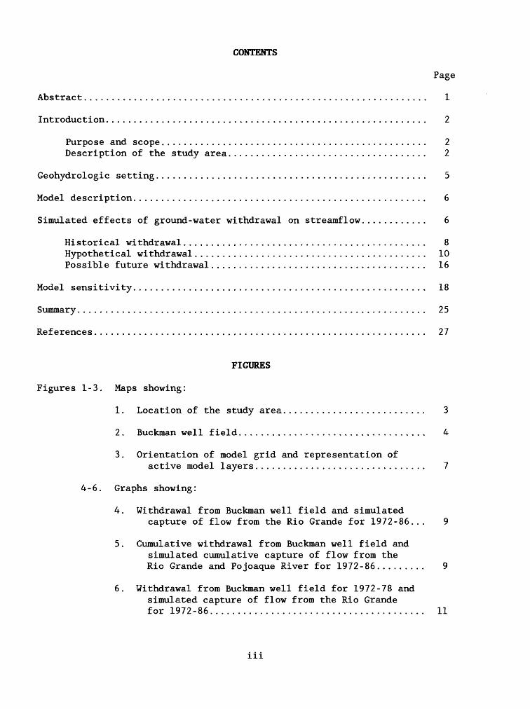
CONTENTS
Page
Abstract.............................................................. 1
Introduction.......................................................... 2
Purpose and scope................................................ 2Description of the study area.................................... 2
Geohydrologic setting................................................. 5
Model description..................................................... 6
Simulated effects of ground-water withdrawal on streamflow............ 6
Historical withdrawal............................................ 8Hypothetical withdrawal.......................................... 10Possible future withdrawal....................................... 16
Model sensitivity..................................................... 18
Summary............................................................... 25
References............................................................ 27
FIGURES
Figures 1-3. Maps showing:
1. Location of the study area.......................... 3
2. Buckman well field.................................. 4
3. Orientation of model grid and representation ofactive model layers ............................... 7
4-6. Graphs showing:
4. Withdrawal from Buckman well field and simulatedcapture of flow from the Rio Grande for 1972-86... 9
5. Cumulative withdrawal from Buckman well field and simulated cumulative capture of flow from the Rio Grande and Pojoaque River for 1972-86......... 9
6. Withdrawal from Buckman well field for 1972-78 and simulated capture of flow from the Rio Grande for 1972-86....................................... 11
111
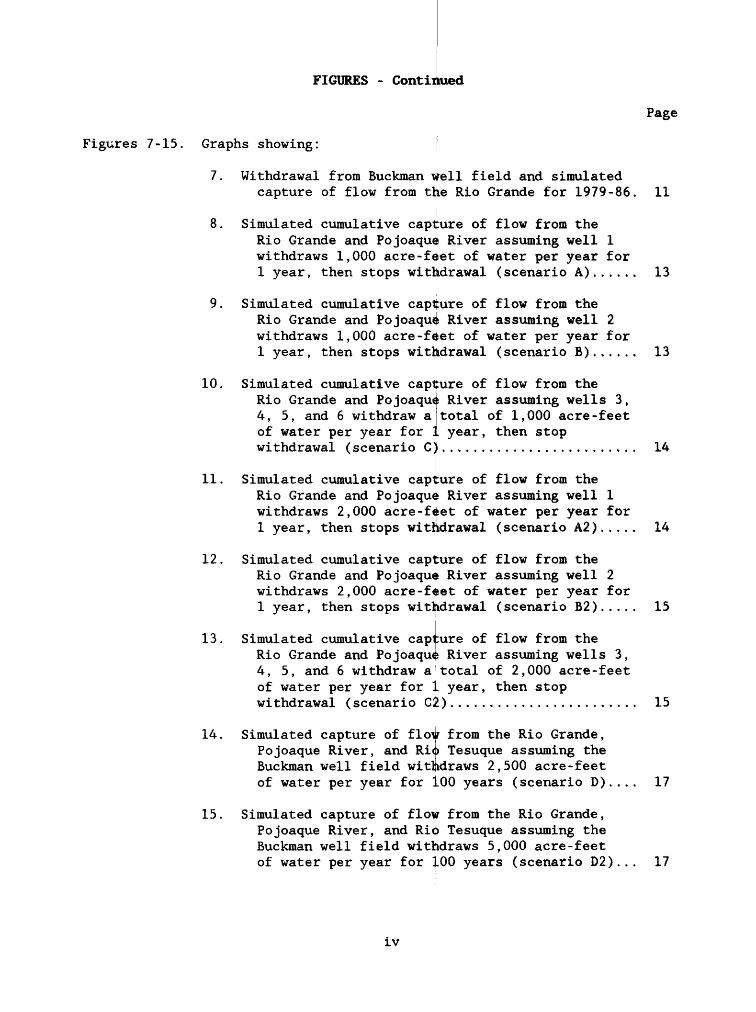
FIGURES - Continued
Figures 7-15. Graphs showing:
7.
8.
9.
10.
11.
12.
13.
14.
15.
Withdrawal from Buckman well field and simulated capture of flow from the Rio Grande for 1979-86
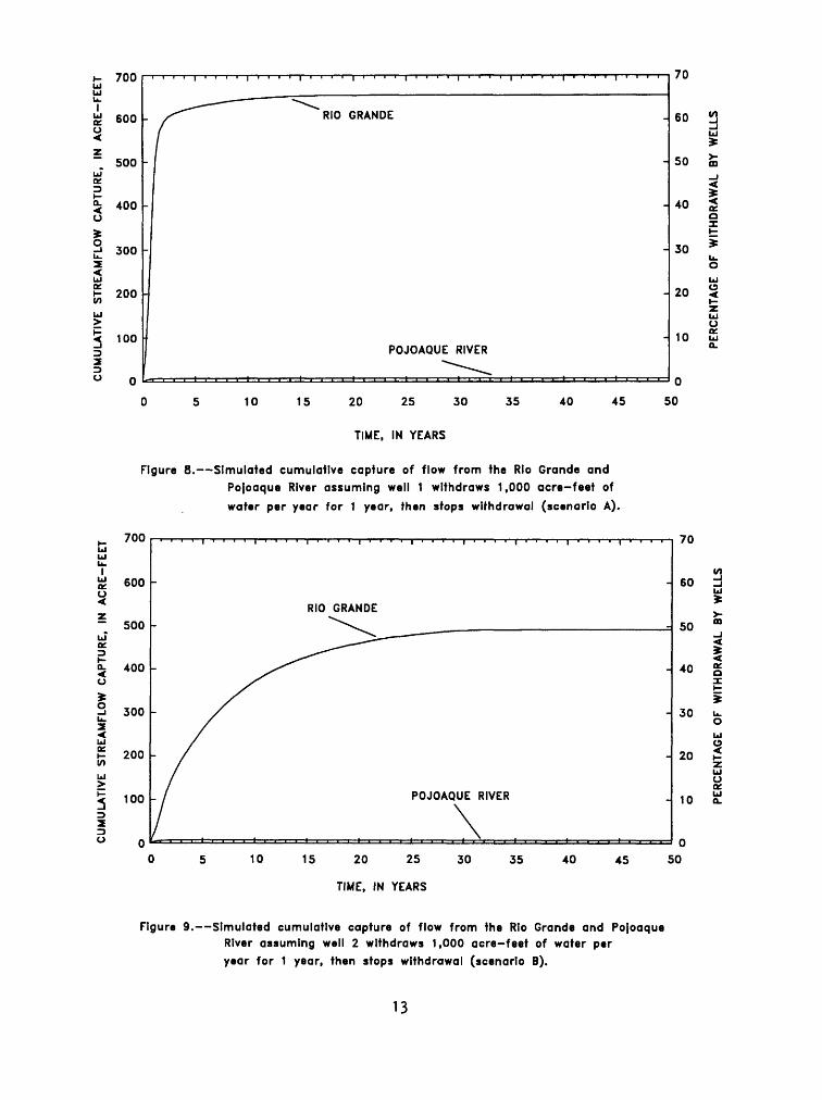
Simulated cumulative capture of flow from the Rio Grande and Pojoaque River assuming well 1 withdraws 1,000 acre-feet of water per year for 1 year, then stops withdrawal (scenario A)......
11
13
Simulated cumulative capture of flow from the Rio Grande and Pojoaque River assuming well 2 withdraws 1,000 acre-feet of water per year for 1 year, then stops withdrawal (scenario B)..... 13
Simulated cumulative capture of flow from the Rio Grande and Pojoaquts River assuming wells 3,4, 5, and 6 withdraw aof water per year for 1 year, then stop withdrawal (scenario C,
captureSimulated cumulative Rio Grande and Pojoaques withdraws 2,000 acre- 1 year, then stops
total of 1,000 acre-feet
14
f«jet
of flow from the River assuming well 1
of water per year for (scenario A2)....,withdrawal 14
Simulated cumulative capture of flow from the Rio Grande and Pojoaquo River assuming well 2 withdraws 2,000 acre-f<jet of water per year for 1 year, then stops withdrawal (scenario B2) 15
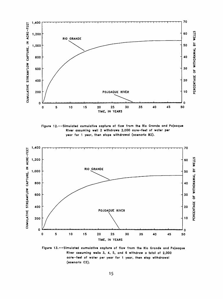
Simulated cumulative capture of flow from the Rio Grande and Pojoaqu^ River assuming wells 3, 4, 5, and 6 withdraw a total of 2,000 acre-feet of water per year for 1 year, then stop withdrawal (scenario C2)........................ 15
Simulated capture of flow from the Rio Grande, Pojoaque River, and Rio Tesuque assuming the Buckman well field withdraws 2,500 acre-feet of water per year for 100 years (scenario D).
Simulated capture of flow from the Rio Grande, Pojoaque River, and Rio Tesuque assuming the Buckman well field withdraws 5,000 acre-feet of water per year for 100 years (scenario D2)
17
17
IV
FIGURES - Concluded
Page
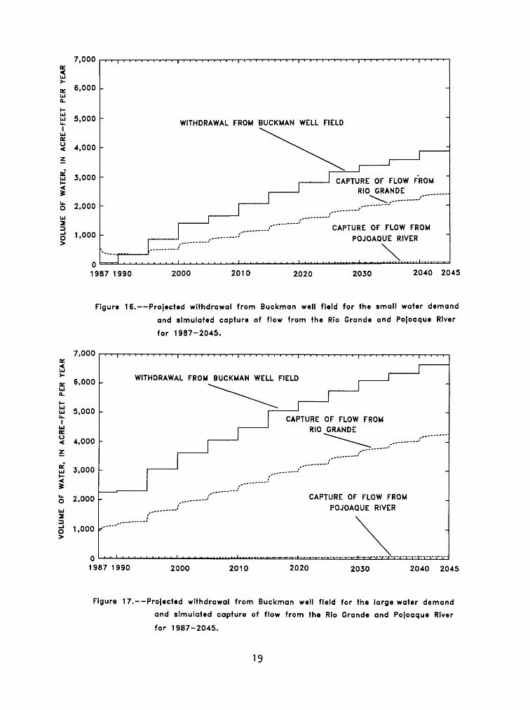
Figure 16. Graph showing projected withdrawal from Buckman well field for the small water demand and simulated capture of flow from the Rio Grande and Pojoaque River for 1987-2045........................................... 19
17. Graph showing projected withdrawal from Buckman well field for the large water demand and simulated capture of flow from the Rio Grande and Pojoaque River for 1987-2045........................................... 19
18. Map showing rediscretized model grid...................... 20
19-23. Graphs showing:
19. Difference in simulated streamflow capture betweenthe rediscretized model and the original model forthe 1972-86 historical period...................... 22
20. Difference in simulated streamflow capture between the rediscretized model and the original model assuming well 1 withdraws 1,000 acre-feet of water per year for 1 year, then stops withdrawal (scenario A)....................................... 22
21. Difference in simulated streamflow capture between the rediscretized model and the original model assuming well 2 withdraws 1,000 acre-feet of water per year for 1 year, then stops withdrawal (scenario B)....................................... 23
22. Difference in simulated streamflow capture between the rediscretized model and the original model assuming wells 3, 4, 5, and 6 withdraw a total of 1,000 acre-feet of water per year for 1 year, then stop withdrawal (scenario C).................. 23
23. Difference in simulated streamflow capture between the rediscretized model and the original model assuming the Buckman well field withdraws 2,500 acre-feet of water per year for 100 years (scenario D)....................................... 24
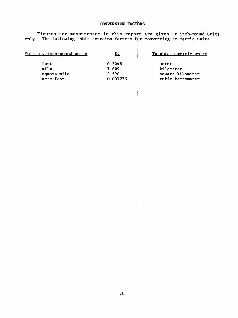
CONVERSION FACTORS
Figures for measurement in this report are given in inch-pound units only. The following table contains factors for converting to metric units.
Multiply inch-pound units
foot milesquare mile acre-foot
0.30481.6092.5900.001233
To obtain metric units
meter kilometer square kilometer cubic hectometer
VI
SIMULATION OF THE EFFECTS OF GROUND-WATER WITHDRAWAL
FROM A WELL FIELD ADJACENT TO THE RIO GRANDE,
SANTA FE COUNTY, NEW MEXICO
By Douglas P. McAda
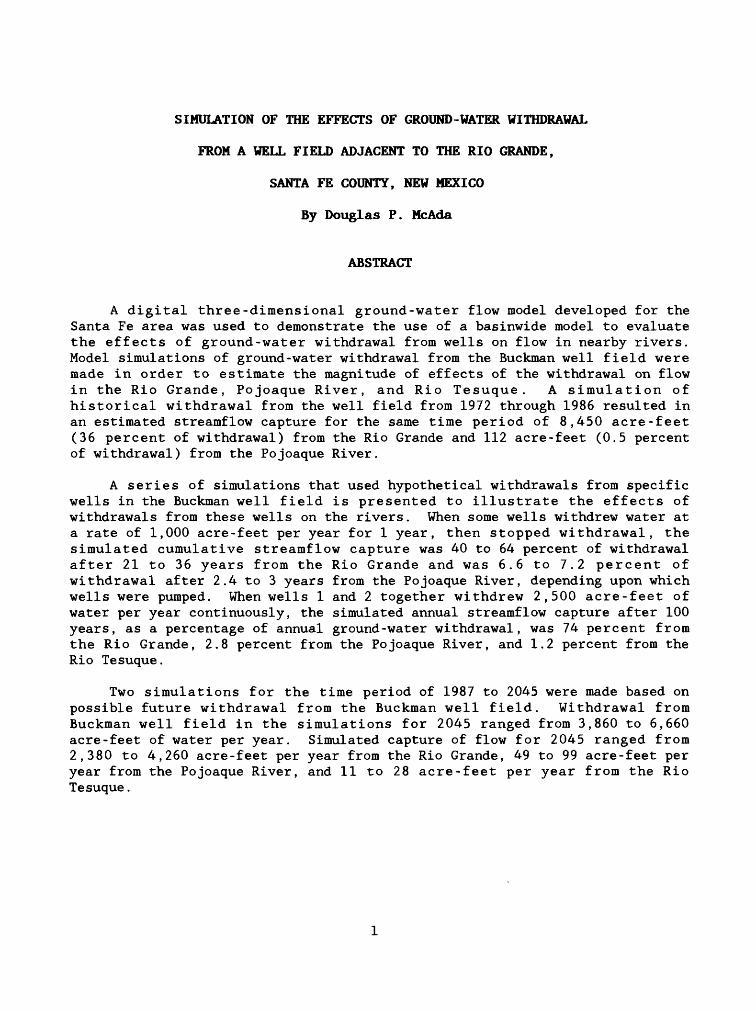
ABSTRACT
A digital three-dimensional ground-water flow model developed for the Santa Fe area was used to demonstrate the use of a basinwide model to evaluate the effects of ground-water withdrawal from wells on flow in nearby rivers. Model simulations of ground-water withdrawal from the Buckman well field were made in order to estimate the magnitude of effects of the withdrawal on flow in the Rio Grande, Pojoaque River, and Rio Tesuque. A simulation of historical withdrawal from the well field from 1972 through 1986 resulted in an estimated streamflow capture for the same time period of 8,450 acre-feet (36 percent of withdrawal) from the Rio Grande and 112 acre-feet (0.5 percent of withdrawal) from the Pojoaque River.
A series of simulations that used hypothetical withdrawals from specific wells in the Buckman well field is presented to illustrate the effects of withdrawals from these wells on the rivers. When some wells withdrew water at a rate of 1,000 acre-feet per year for 1 year, then stopped withdrawal, the simulated cumulative streamflow capture was 40 to 64 percent of withdrawal after 21 to 36 years from the Rio Grande and was 6.6 to 7.2 percent of withdrawal after 2.4 to 3 years from the Pojoaque River, depending upon which wells were pumped. When wells 1 and 2 together withdrew 2,500 acre-feet of water per year continuously, the simulated annual streamflow capture after 100 years, as a percentage of annual ground-water withdrawal, was 74 percent from the Rio Grande, 2.8 percent from the Pojoaque River, and 1.2 percent from the Rio Tesuque.
Two simulations for the time period of 1987 to 2045 were made based on possible future withdrawal from the Buckman well field. Withdrawal from Buckman well field in the simulations for 2045 ranged from 3,860 to 6,660 acre-feet of water per year. Simulated capture of flow for 2045 ranged from 2,380 to 4,260 acre-feet per year from the Rio Grande, 49 to 99 acre-feet per year from the Pojoaque River, and 11 to 28 acre-feet per year from the Rio Tesuque.

INTRODUCTION!
Many alluvial-hasin aquifers in New Mexibo are hydraulically connected to perennial rivers. The relation of ground water and surface water is a major consideration in management of the water resources of these basins. Because the water of most rivers in New Mexico is fully appropriated it is important to evaluate the effects of ground-water withdrawal from wells adjacent to these rivers on the flow of the rivers.
Basinwide ground-water flow models, which include simulation of the interaction between the aquifer and the major rivers, have been developed for some of the alluvial basins in New Mexico. These models may be a valuable tool for evaluating effects of ground-water Withdrawal from wells on flow in nearby rivers.
Purpose and Scope
This report demonstrates the use of a to provide estimates of the effect of ground- flow in nearby rivers. The Buckman well
basinwide ground-water flow model water withdrawal from wells on field was selected for this study
because of its proximity to major rivers, thej existence of a basinwide model that can simulate the interaction between the aquifer and the major rivers, and the availability of detailed pumping records for the well field. The model used in this report was developed for the Santa Fe area of the Espanola Basin by McAda and Wasiolek (1988). i
Description of the Squdy Area
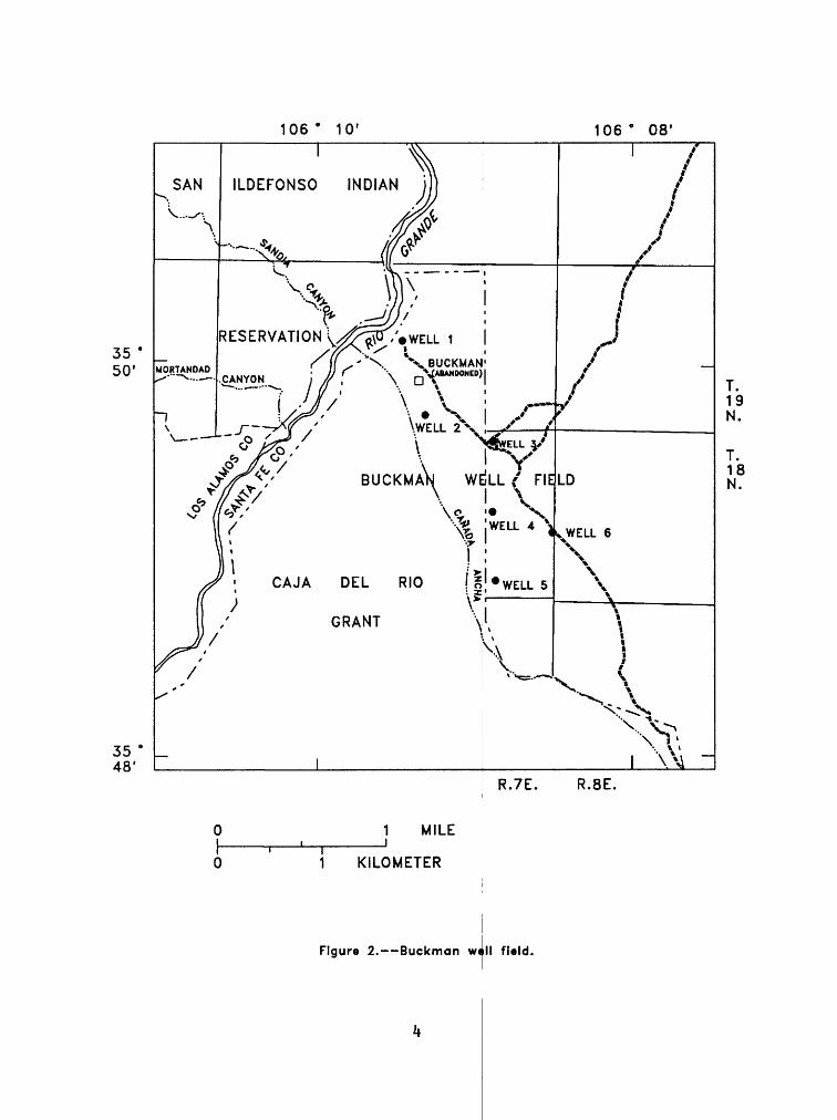
The Buckman well field was put into operation in July 1972 to increase the water supply for the city of Santa F^, New Mexico. The well field is about 15 miles northwest of Santa Fe, near the abandoned town of Buckman on the east side of the Rio Grande (fig. 1).shown in figure 2. The production wells are1.5 miles (well 6) from the Rio Grande.the Rio Grande, is about 5 miles north of tho well field. The Rio Tesuque,tributary of the Pojoaque River, is about 9 miles east of the well field.
A map of the well-field area is about 600 feet (well 1) to about
The Pojoaque River, a tributary ofa
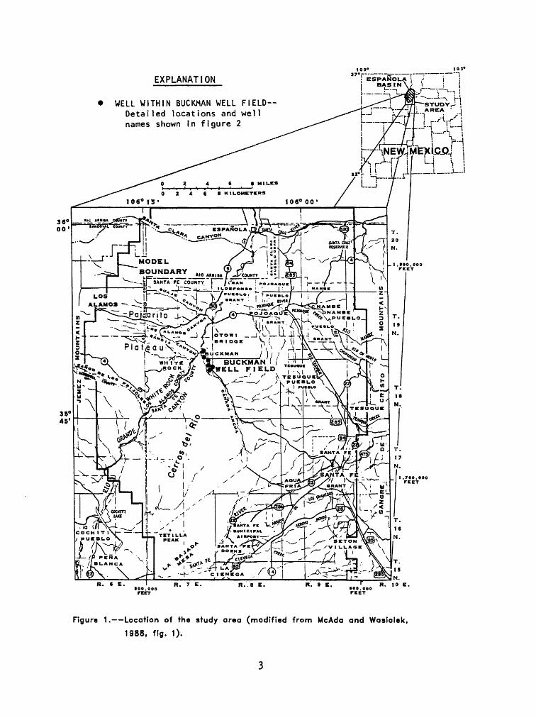
EXPLANATION
WELL WITHIN BUCKMAN WELL FIELD Detailed locations and well names shown in figure 2
BUCKMAN WELL FIELD
Figure 1. Location of the study area (modified from McAda and Wasiolek,
1988, fig. 1).
106° 10' 106 ° 08'
35 * 50'
RESERVATION I ///-<& /.WELL 1" I j :\ BUCKMAN 1
** "V f ARAM Dfiurnl I
35 ' 48'
\WELL
\
ILDEFONSO INDIAN
*
BUCKMA WELL / FIEiilWELL 4 \
CAJA DEL RIO
GRANT
o|»WELL 5
V \\
7
f
LD
KWELL 6
\\
R.7E. R.8E.
T.19N.
T.18N.
MILE
KILOMETER
Figure 2. Buckman well ffeld
GEOHYDROLOGIC SETTING
A description of the geologic framework of the Santa Fe area model is given by McAda and Wasiolek (1988, p. 7-12). Detailed descriptions of the geology of the area are given by Spiegel and Baldwin (1963), Griggs (1964), Galusha and Blick (1971), Baltz (1978), Kelley (1978), and Manley (1978a, b).
The Buckman wells produce water from the Tertiary Tesuque Formation of the Santa Fe Group, the principal aquifer in the area. As described by Spiegel and Baldwin (1963, p. 39), the Tesuque Formation "consists of several thousand feet of pinkish-tan soft arkosic, silty sandstone and minor conglomerate and siltstone." The Tesuque Formation crops out to the east and northeast of the well field. Both west of the Rio Grande and south of the well field, Quaternary and Tertiary volcanic roqks overlie the Tesuque Formation. Quaternary alluvium covers the Tesuque Formation in much of the immediate area of the well field.
The thickness of the Tesuque Formation was estimated to be greater than 8,000 feet near the Rio Grande by Kelley (1978) and greater than 3,700 feet in the deepest parts of the basin by Galusha and Blick (1971, p. 44). McAda and Wasiolek (1988, p. 64) showed that the Santa Fe area model was not significantly affected by a change in maximum aquifer saturated thickness from 5,600 to 3,800 feet. Therefore, it is not critical to the model simulations if either of the thickness estimates is correct.
The Santa Fe area model includes the Tesuque aquifer system, which is defined by McAda and Wasiolek (1988, p. 7-12) as the Tertiary Tesuque, Puye, and Ancha Formations of the Santa Fe Group. The Puye Formation (Griggs, 1964, p. 28; Purtymun and Johansen, 1974, p. 347-349) overlies the Tesuque Formation in the area of Los Alamos on the west side of the Rio Grande. The Puye Formation primarily consists of sand and gravel, and its thickness is as much as 700 feet. The Ancha Formation (Spiegel and Baldwin, 1963, p. 45) overlies the Tesuque Formation south and west of the city of Santa Fe. The Ancha Formation primarily consists of fine to coarse gravel and minor silt and sand, and its thickness is as much as 300 feet. The hydrology of the Tesuque aquifer system as represented in the Santa Fe area model as well as references to other reports that discuss the hydrology of the area is given by McAda and Wasiolek (1988, p. 12-15).
Most recharge to the Tesuque aquifer system east of the Rio Grande occurs near the Sangre de Cristo Mountains by infiltration of streamflow and precipitation through fractured bedrock and alluvial streambeds (McAda and Wasiolek, 1988, p. 13). In comparison, direct recharge to the outcrops of the Tesuque and Ancha Formations is small, but probably occurs during periods of heavy precipitation as infiltration from ephemeral streams. The primary direction of ground-water flow on the east side of the Rio Grande is westward toward the river. The main discharge area for the Tesuque aquifer system is the Rio Grande. A smaller amount of water discharges from the aquifer system to the Pojoaque River and its tributaries to the north and the Santa Fe River and Cienega Creek to the south. Some water discharges to the southwest from the basin as underflow.
Recharge to the Tesuque aquifer system west of the Rio Grande is by infiltration of streamflow and precipitation through the overlying volcanic rocks of the Jemez Mountains and Pajarito Plateau, and through stream bottoms incised into the Puye and Tesuque Formations (McAda and Wasiolek, 1988, p. 13). Underflow from the Jemez Mountains also provides recharge to the aquifer system. The ground water moves southeastward to the Rio Grande, where it discharges.
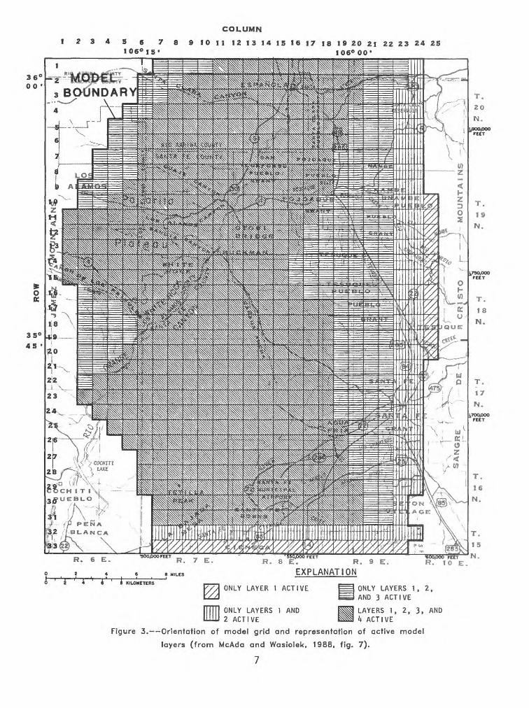
MODEL DESCRIPTION
The three-dimensional finite-difference developed for the Santa Fe area by McAda and in detail in that report (p. 16-33). The was developed by McDonald and Harbaugh I procedure (SIP) was used to solve the finite- ground-water flow equation (McDonald and
model used for this study was Wasiolek (1988) and is described
computer program used for this model 1988). The strongly implicit
difference approximation to the 1988, p. 12-1 - 12-29).Harbaugh
The model consists of four layers with a uniform horizontal grid spacing.Each grid cell represents a 1-square-mile block of the aquifer (fig. 3). The topmost layer of the model was assumed to represent the upper 800 feet of the aquifer, the second layer was assumed to represent 1,200 feet, and the third and fourth (lowermost) layers were assumed to each represent 1,800 feet. The topmost layer represents the unconfined part of the aquifer and the lower three layers represent the confined part of the aquifer. The layers do not represent specific units within the aquifer system, but allow the discretization of the aquifer system into thrcie dimensions. A discussion of the boundaries and hydrologic characteristics of the Tesuque aquifer system and the representation of them in the model i.s given by McAda and Wasiolek (1988, p. 17-33).
The initial conditions used in the simulations were those obtained from the calibrated steady-state Santa Fe area model. The Buckman well-field withdrawals were the only stresses applied to these initial conditions. The effects of the withdrawals on streamflow were evaluated by comparing the water budgets of the rivers simulated with withdrawals to the water budgets of the rivers simulated with steady-state conditions.
SIMULATED EFFECTS OF GROUND-WATER WITHDRAWAL ON STREAMFLOW
Water withdrawn from a well comes initially from storage within the aquifer. Removal of water creates a cone of depression in the potentiometrie surface that spreads and creates a gradient in the surface toward the well. If that cone of depression intersects a river that is in hydraulic connection with the aquifer, the withdrawal of water from the well will have an effect on flow in the river. That effect can be either an increase in recharge from the river to the aquifer or a decrease in discharge from the aquifer to the river. In either case, the result is capture of streamflow.
There is a time lag between initial withdrawal of water from a well and the beginning of streamflow capture. This time lag is dependent upon the hydrologic characteristics of the aquifer atid the distance of the well from the river. After withdrawal of water from thej well has stopped, the effect of the withdrawal on the river will continue until the potentiometric head in the aquifer near the river returns to its condition prior to the time that withdrawal began.
8 9 10 II 12 13 14 IS 16 17 18 19 20 21 22 23 24 25
45
oc-^T
R. 6 E.
2 4
R. 7 E.
8 MILES
'550,OOO FEETR. 8 E. R. 9 E.
EXPLANATION
600000 FEET N.R- io E .
468 KILOMETERS m ONLY LAYER 1 ACTIVE
ONLY LAYERS 1 AND 2 ACTIVE
ONLY LAYERS 1,2, AND 3 ACTIVE
LAYERS 1, 2, 3, AND k ACTIVE
Figure 3. Orientation ot model grid and representation ot active model
layers (from McAda and Wasiolek, 1988, fig. 7).
7
Historical Withdrawal
Monthly historical withdrawal from th,e Buckman well field, from the beginning of production in July 1972 through December 1986, was simulated using the Santa Fe area model. Initial conditions for the simulation were the conditions resulting from the calibrated ^steady-state model. The Buckman well-field withdrawal was the only stress applied to these steady-state conditions. j
Withdrawal records for the well field 'were provided by the Sangre de Cristo Water Company and the New Mexico State Engineer Office (files of New Mexico State Engineer Office, Albuquerque). Prior to 1976, withdrawal was reported as a monthly total for the entire well field. Since 1976, withdrawals have been reported by well on a .monthly basis. The withdrawal that occurred before 1976 was simulated by assuming that the withdrawal was distributed among existing production wells (wells 3, 4, 5, and 6) in the same relative proportions as withdrawal from 1976 'through 1978.
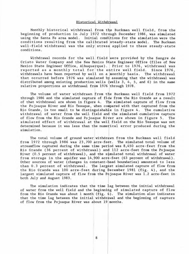
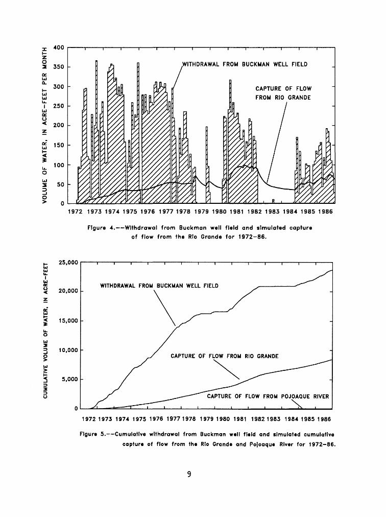
The volume of water withdrawn from the Buckman well field from 1972 through 1986 and the simulated capture of flow from the Rio Grande as a result of that withdrawal are shown in figure 4. Ttye simulated capture of flow from the Pojoaque River and Rio Tesuque, when compared with that captured from the Rio Grande, is too small to be distinguishable in figure 4. The cumulative withdrawal of water from the well field and the simulated cumulative capture of flow from the Rio Grande and Pojoaque River are shown in figure 5. The simulated effect of withdrawal at the well field on the Rio Tesuque was not determined because it was less than the numerical error produced during the simulation.
The total volume of ground water withdrawn from the Buckman well field from 1972 through 1986 was 23,700 acre-feet. The simulated total volume of streamflow captured during the same time period was 8,450 acre-feet from the Rio Grande (36 percent of withdrawal) and 112 acre-feet from the Pojoaque River (0.5 percent of withdrawal), and the simulated total withdrawal of water from storage in the aquifer was 14,900 acre-feet (63 percent of withdrawal). Other sources of water (changes in constant-head boundaries) amounted to less than 0.3 percent of withdrawal. The largest simulated capture of flow from the Rio Grande was 100 acre-feet during December 1981 (fig. 4), and the largest simulated capture of flow from the Pojoaque River was 1.2 acre-feet in both July and August 1983.
The simulation indicates that the time lag between the initial withdrawal of water from the well field and the beginning of simulated capture of flow from the Rio Grande was about 1 month (fig. 4). The simulation also indicates that the time lag between the initial withdrawal and the beginning of capture of flow from the Pojoaque River was about 19 months.
z o
UJ Q.
UJ UJu.
IUJ OS U
OS UJ
UJ2E
400
350 - WITHDRAWAL FROM BUCKMAN WELL FIELD
CAPTURE OF FLOW
FROM RIO GRANDE
1972 1973 1974 1975 1976 1977 1978 1979 1980 1981 1982 1983 1984 1985 1986
Figure 4. Withdrawal from Buckman well field and simulated capture
of flow from the Rfo Grande for 1972-86.
Ul Ulu.I
uiD£ U
25,000
20,000 -
15,000 -
10,000 -
5,000 -
WITHDRAWAL FROM BUCKMAN WELL FIELD
CAPTURE OF FLOW FROM RIO GRANDE
CAPTURE OF FLOW FROM POJOAQUE RIVER
1972 1973 1974 1975 1976 19771978 1979 1980 1981 19821983 1984 1985 1986
Figure 5. Cumulative withdrawal from Buckman well field and simulated cumulative
capture of flow from the Rio Grande and Pofoaque River for 1972-86.
Streamflow capture caused by withdrawal will continue for a period of time even if
from the well field prior to 1987 withdrawal from the well field
ceases. The continued loss of water by the rivers will replenish some of the water that was withdrawn from storage within the aquifer. To demonstrate the continuation of Streamflow capture after pumping has ended, the preceding simulation was divided into two separate simulations. One simulated withdrawal through 1978 and the second simulated withdrawal from 1979 through1986. Prior to 1979, wells 3, 4, 5, and 6, Grande than wells 1 and 2 (fig. 2), were the
which are farther from the Rio only production wells. In 1979,
wells 1 and 2 went into production and the older wells were subsequently used very little.
The withdrawal of water from the Buckman well field and the resulting simulated capture of flow from the Rio Grande are shown in figures 6 and 7. The simulated capture of flow from the Pojoaque River is too small in comparison with that from the Rio Grande to be distinguishable in these figures. In the first of these simulations, the capture of flow from the Rio Grande was substantial 8 years after withdrawal from the well field had ceased (fig. 6). The recession curve for capture of flow from the Rio Grande in the first simulation (fig. 6) can be compared with the recession curve for the interval from 1982 to 1984 in the second simulation (fig. 7). In the second simulation, the decrease of capture of flow from the Rio Grande was more rapid after withdrawal ceased than in the first simulation because wells 1 and 2 are closer to the river than wells 3, 4, 5, and 6. Figures 6 and 7 also show that the effects of withdrawals on the Rio Grande occur more rapidly and are greater from wells 1 and 2 than from wells 3, 4, 5, and 6. Because the Rio Grande remains in hydraulic continuity with the aquifer during these simulations (simulated hydraulic head does not fall below the elevation of the bottom of the riverbed) , the Streamflow capture caused by withdrawal fromwells 1 and 2 (fig. 7) can be superimposed on withdrawal from wells 3, 4, 5, and 6 (fig. 6) capture for the combined simulation shown in
the Streamflow capture caused by The result is the Streamflow
figure 4.
Hypothetical Withdrawal
To further illustrate the magnitudes of the effects of withdrawal from particular wells in the Buckman well field on the flow of the rivers, three series of hypothetical scenarios were simulated. The first series of hypothetical scenarios included the assumptions that particular wells would be pumped at a combined constant rate of 1,000 kcre-feet of water per year for 1 year, and that pumping then would cease. Each simulation was for a 100-year period. The three simulations of the first series of scenarios were for well 1 pumping (scenario A), well 2 pumping (scenario B), and wells 3, 4, 5, and 6 pumping (scenario C). The initial conditions for each of these simulations were the same"as those obtained from the calibrated steady-state Santa Fe area model (McAda and Wasiolek, 1988). For this and the next series of hypothetical simulations, the effect of withdrawal from the Buckman well field on the Rio Tesuque was not determined because it was less than the numerical error involved in the simulations. ,
10

z o
LJ Q_
LJ LJ
LJ
O
or LJ
O
LJ
O>
400
350
300
250
200
150
100
50
WITHDRAWAL FROM BUCKMAN WELL FIELD
(WELLS 3, 4, 5, AND 6)
CAPTURE OF FLOW
FROM RIO GRANDE
1972 1973 1974 1975 1976 1977 1978 1979 1980 1981 1982 1983 1984 1985 1986
Figure 6. Withdrawal from Buckman well field for 1972-78 and simulated capture of flow from the Rio Grande for 1972-86.
z o2E orLJa.
Di O
or LJi-
o>
WITHDRAWAL FROM BUCKMAN WELL FIELD
(PRIMARILY WELLS 1 AND 2)
1972 1973 1974 1975 1976 1977 1978 1979 1980 1981 1982 1983 1984 1985 1986
Figure 7. Withdrawal from Buckman well field and simulated capture of flow from the Rio Grande for 1979-86.
11
The cumulative streamflow capture for eiach of the simulations in the first series is shown in figures 8 through 10. As can be seen from these figures, the closer the wells are to the Rio G'rande, the more rapid is capture of flow from the river and the larger is the total volume of water captured. From the simulation with well 1 pumping (fig. 8), 59 percent of the total withdrawal by the well was captured from the Rio Grande in the first 2 years and the maximum of 65 percent of the withdrawal was captured from the Rio Grande after 20 years. This simulation also estimated that 0.76 percent of the withdrawal by well 1 was captured from the Pojoaque River in the first 2 years and the maximum of 0.78 percent of the withdrawal was captured from the Pojoaque River after 2.4 years. From the stimulation with well 2 pumping (fig. 9), 14 percent of the total withdrawal by the well was captured from the Rio Grande in the first 2 years and the maximum of 49 percent of the withdrawal was captured from the Rio Grande after 36 years. This simulation also estimated that 0.74 percent of the withdrawal by well 2 was captured from the Pojoaque River in the first 2 years and the maximum of 0.75 percent of the withdrawal was captured from the Pojoaque River after 2.4 years. From the simulation with wells 3, 4, 5, and 6 pumping (fig. 10), 11 percent of the total withdrawal by the wells was captured from the Rio Grande in the first 2years and the maximum of 41 percent of theRio Grande after 32 years. This simulation also estimated that 0.76 percent of the withdrawal by the wells was captured from the Pojoaque River in thefirst 2 years and the maximum of 0.81 percent from the Pojoaque River after 3 years.
withdrawal was captured from the
of the withdrawal was captured
A second series of hypothetical simulations (scenarios A2, B2, and C2) was the same as the first series except that the rate of pumping was 2,000 acre-feet per year for 1 year. The simulated cumulative streamflow capture for each of the simulations in the second series is shown in figures 11 through 13. The simulated cumulative streamflow capture for these simulations, as a percentage of withdrawal by the wells, is similar to those with the lesser rate of withdrawal (figs. 8 through 10), except that the total percentage of withdrawal that was captured from the Rio Grande was slightly larger and the time until streamflow capture Ceased was slightly longer. From the simulation with well 1 pumping (figi 11), 67 percent of the total withdrawal by the well was captured from the Rio Grande after 29 years and 0.39 percent of the withdrawal was captured from the Pojoaque River after 3 years. From the simulation with well 2 pumping (fig. 12), 54 percent of the total withdrawal by the well was captured from the Rio Grande after 43 years and 0.36 percent of the withdrawal was captured from the Pojoaque River after 2.4 years. From the simulation with wells 3, 4, 5, and 6 pumping (fig. 13), 46 percent of the total withdrawal by the wells was captured from the Rio Grande after 47 years and 0.39 percent of the withdrawal was captured from the Pojoaque River after 2.4 years.
12
CU
MU
LATI
VE
S
TRE
AM
FLO
W
CA
PTU
RE
, IN
A
CR
E-F
EE
TC
UM
UL
AT
IVE
S
TRE
AM
FLO
W
CA
PT
UR
E,
IN
AC
RE
-FE
ET
ZJ 10 c I I
?
lo
5 E.
"
*
Q
2 2
I
O> o
o
3 I Q
a .-
8 a
laIT
Q
3o
q _H
«
3
=ri
i*o
2.
oS
o
o^ -
2 M ~«
Q_
3 O Q
.0 C
(D
K)
O
m JO
«Q C a
00
so
c
*<
~
3
<
3Q
<D
C
«
"
o-.
. o
:£
o
M
<
- < «
3S
=
o
» *
3 "*?
H
1 - a
r -
5 §
2
Q_
O
o .>
O
O
L>
^*
~*
o JO
o
O <_ o
o
o
o
o
o
o
o
PE
RC
EN
TA
GE
O
F
WIT
HD
RA
WA
L B
Y
WE
LLS
o>
o0
00
00
PER
CEN
TAG
E O
F W
ITH
DR
AW
AL
BY
WEL
LS

70°IK 600
500
< 400u
300
200
100
RIO GRANGE
POJOAQUE RIVER
10 15 20 25
TIME, IN YEARS
30 35 45
70
60
50 m
40
30
20
10
50
Figure 10. Simulated cumulative capture of flow from the Rio Grande and Pojoaque
River assuming wells 3, 4, 5, and 6 withdraw a total of 1,000
acre-feet of water per year for 1 year, then stop withdrawal
(scenario C).
u a:
,400
1,200 -
1,000 -
800 -
600 -
400
200 POJOAQUE RIVER
10 15 20 25
TIME, IN YEARS
Figure 11. Simulated cumulative capture of
Pojoaque River assuming well 1
water per year for 1 year, then
35 40 45
flow
70
60
50
40
30
20
10
50
from the Rio Grande and
withdraws 2,000 acre-feet of
stops withdrawal (scenario A2).
CU
MU
LA
TIV
E
ST
RE
AM
FL
OW
C
AP
TU
RE
, IN
A
CR
E-F
EE
TC
UM
UL
AT
IVE
S
TR
EA
MF
LO
W
CA
PT
UR
E,
IN
AC
RE
-FE
ET
IT
9 2
3
n °
< c
5 7
* °
0 -*
o
2.
«
5 Q-
o
w c 2
0
o 3
£10
S.
5.
3
"iU
A
*
-*
- o
*
5,
" °
=o
o
'
O
o
1
E.
Q
J"
O
Q.
Q.
-H .
o
ro
o
I §
s.o
-
^
S
3
-«
T
Q-*._!»'
° 8
o.-S
o
S £
£
.o
~
c
3"
M
-*
Q.
o"
« 3-
3
I A
Q
-*=-
?
2
05.?
5 o
°
IO
-fc
T o Q
X
t C
10-<
01
m 70 I/I
04 o
o
o
o
o
o
o
PE
RC
EN
TAG
E
OF
WIT
HD
RA
WA
L BY
W
ELL
SPE
RC
ENTA
GE
OF
WIT
HD
RA
WA
L BY
W
ELL
S
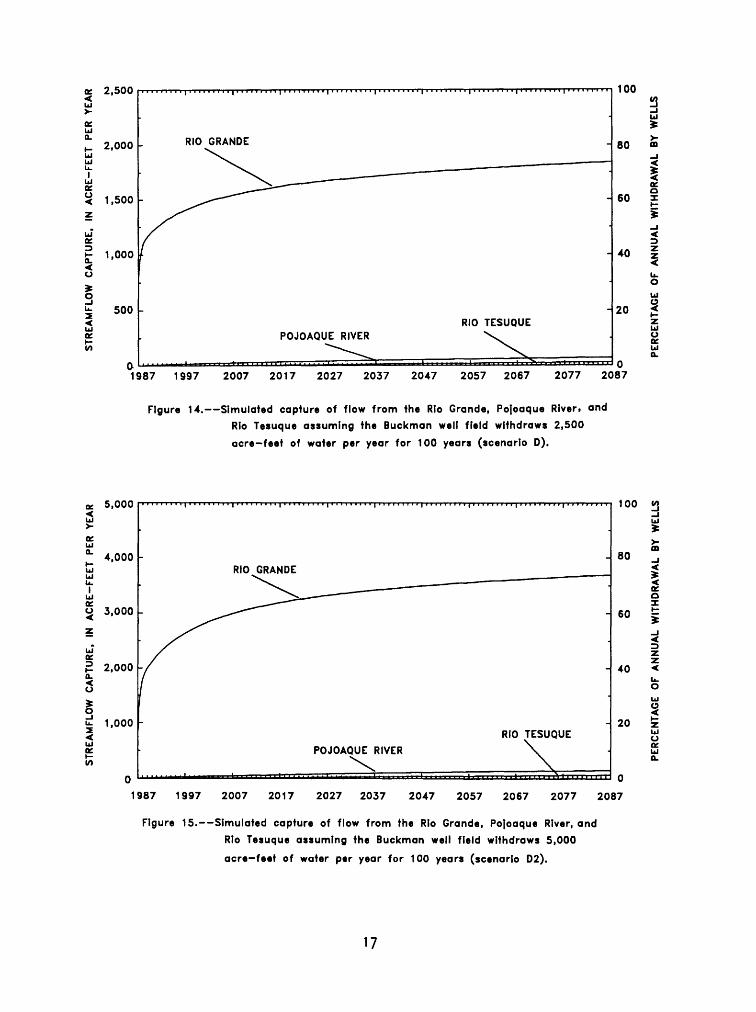
For the third and last series of hypothetical simulations, the Buckman well field was assumed to withdraw water first at a constant rate of 2,500 acre-feet per year for 100 years (scenario D) and second at 5,000 acre-feet per year for 100 years (scenario D2). It was assumed that well 1 produced 40 perc«nt and well 2 produced 60 percent of the total withdrawal of water. These proportions approximately correspond to those reported in the withdrawal records of the well field in recent years. The initial conditions of the aquifer for these simulations were the conditions resulting from the simulation of historical withdrawals described under "Historical withdrawal" and shown in figure 4 of this report.
The capture of flow from the Rio Grande, Pojoaque River, and Rio Tesuque for this final series of hypothetical simulations is shown in figures 14 and 15. The percentage of annual withdrawal of water from the Buckman well field that is captured from the three rivers is approximately the same for both simulations, particularly after about 30 years of withdrawal. After 100 years of pumping 2,500 acre-feet of water per year from the well field, the simulated annual streamflow capture, in terms of percentage of annual withdrawal, was 74 percent from the Rio Grande, 2.8 percent from the Pojoaque River, and 1.2 percent from the Rio Tesuque (fig. 14). After 100 years of pumping 5,000 acre-feet of water per year from the well field, the simulated annual streamflow capture, in terms of percentage of annual withdrawal, was 74 percent from the Rio Grande, 2.9 percent from the Pojoaque River, and 1.3 percent from the Rio Tesuque (fig. 15). The simulated rates of capture of flow from the rivers still are increasing after 100 years (figs. 14 and 15).
Possible Future Withdrawal
Two simulations of projected withdrawal from the Buckman well field from 1987 to 2045 were made using estimated withdrawal rates reported by the Santa Fe Metropolitan Water Board (1984, table 4-2). The two sets of projected withdrawals are based on the estimated small and large water demands of Santa Fe. The initial conditions for these simulations were the conditions resulting from the simulation of historical withdrawals described previously in this report. Well 1 was assumed to produce 40 percent of the total well-field withdrawal and well 2 was assumed to produce 60 percent of the total.
16
ST
RE
AM
FL
OW
C
AP
TU
RE
, IN
A
CR
E-F
EE
T
PE
R
YE
AR
ST
RE
AM
FL
OW
C
AP
TU
RE
. IN
A
CR
E-F
EE
T
PE
R
YE
AR
Ul
o
o
I I (/>
2
3o
c_
_
P
< o
c<
M 2
a M
»
? I
a O
3
-K«
«
O
* 2-
Q.
K> 8
o
-^ o
- o 3 a.
PE
RC
EN
TA
GE
O
F A
NN
UA
L
WIT
HD
RA
WA
L
BY
W
ELL
SP
ER
CE
NT
AG
E
OF
AN
NU
AL
W
ITH
DR
AW
AL
B
Y
WE
LL
S

The projected withdrawal from the Buckjman well field and the simulated capture of flow from the Rio Grande and Pojoaque River for these two simulations are shown in figures 16 and 17. The simulated capture of flow from the Rio Tesuque is small in comparison and would not be distinguishable in these figures. The reduction in simulated capture of flow from the Rio Grande from 1987 to 1995 in the small water-demand simulation (fig. 16) resulted because the simulated withdrawal for those years was less than the recent historical withdrawal (fig. 4). At the end of the simulation with small water demand, the Buckman well-field withdrawal was 3,860 acre-feet per year, and the streamflow capture was 2,380 acre-feet per year from the Rio Grande, 49 acre-feet per year from the Pojoaque River, and 11 acre-feet per year from the Rio Tesuque. At the end of the simulation with large water demand, the Buckman well-field withdrawal was 6,660 acre-feet per year, and the streamflow capture was 4,260 acre-feet per year from the Rio Grande, 99 acre-feet per year from the Pojoaque River, and 28 acre-feet per year from the Rio Tesuque.
MODEL SENSITIVITY
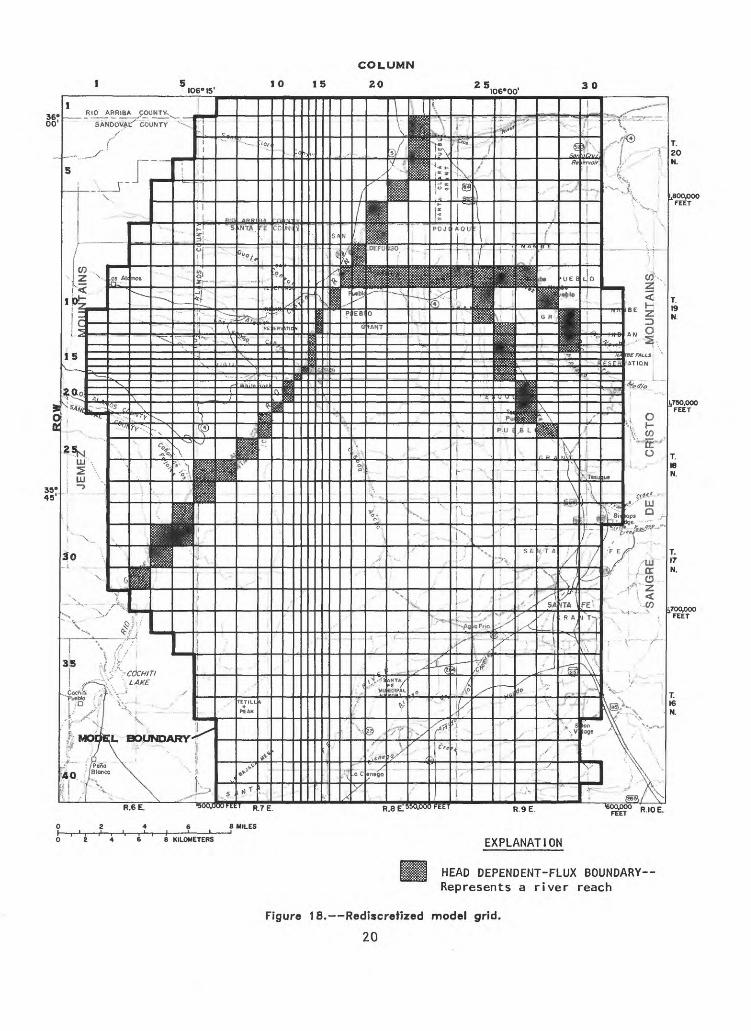
As noted earlier in this report, the scope of this study was limited to the use of an existing ground-water flow model developed for the Santa Fe area (McAda and Wasiolek, 1988). The Santa Fe area model is a regional model of the Tesuque aquifer system and was not developed specifically for estimating the effects of ground-water withdrawal from the Buckman well field on streamflow. A model developed specifically for that objective would likely have a more detailed grid spacing for the area of the well field and thinner upper layers than the Santa Fe area model. Therefore, the sensitivity of the simulated effects of withdrawal to changes in the model grid and layers was tested.
The sensitivity of simulated effects of withdrawal to refinement of the model grid was tested by reducing the grid-cell dimensions near the well field and dividing each of the two upper model layers into two layers. The horizontal dimensions of the rediscretized model grid are shown in figure 18. The horizontal grid spacing was reduced from 1 mile to 1/3 mile in and near the Buckman well field. The grid spacing increases with increasing distance from the well field until it reaches the dimensions of the original Santa Fe area model. The upper layer of the original model was divided into an upper 300-foot-thick layer (layer 1) and a 500-fodt-thick layer (layer 2). The second layer of the original model was divided into two 600-foot-thick layers (layers 3 and 4). The thickness for the remaining two layers of the original model remained unchanged. The other characteristics of the rediscretized model were kept as similar as possible to those of the original model. The vertical to horizontal anisotropy ratio, used to calculate the vertical hydraulic conductivity between the new layers added to the model, was the same as that used between the original layers (0.01). The ground-water withdrawal from each Buckman well was proportioned into the new model layers on the basisof the lithologic logs (and velocity profilesThe most aquifer discharge in the well field for the rediscretized model was from layer 3. The least discharge was from layer 1.
18
where available) of each well.
7,000
WITHDRAWAL FROM BUCKMAN WELL FIELD
CAPTURE OF FLOW FROM RIO GRANDE
CAPTURE OF FLOW FROM
POJOAQUE RIVER
1987 1990 2000 2010 2020 2030 2040 2045
Figure 16. Projected withdrawal from Buckman well field for the small water demand
and simulated capture of flow from the Rio Grande and Pojoaque River
for 1987-2045.
7,000
K 6,000LJ Q.
ui 5,000
OS
< 4,000
5 3,000<
o 2,000
^ 1,000>
WITHDRAWAL FROM BUCKMAN WELL FIELD
1987 1990
CAPTURE OF FLOW FROM RIO GRANDE
CAPTURE OF FLOW FROM POJOAQUE RIVER
2000 2010 2020 2030 2040 2045
Figure 17.--Projected withdrawal from Buckman well field for the large water demand
and simulated capture of flow from the Rio Grande and Pojoaque River
for 1987-2045.
19
30
R.6E. 700,000 FEET p j £
6 8 MILES
R-IOE.
2468 KILOMETERS EXPLANATION
HEAD DEPENDENT-FLUX BOUNDARY Represents a river reach
Figure 18. Rediscretized model grid.
20
The smaller grid spacing in the area of the Buckman well field resulted in more accurately modeled locations of the individual wells in relation to the Rio Grande. The division of the original model layers into smaller upper layers resulted in reduced vertical hydraulic connection between the model layers in which most of the simulated withdrawal occurs (rediscretized model layers 2 and 3) and the Rio Grande.
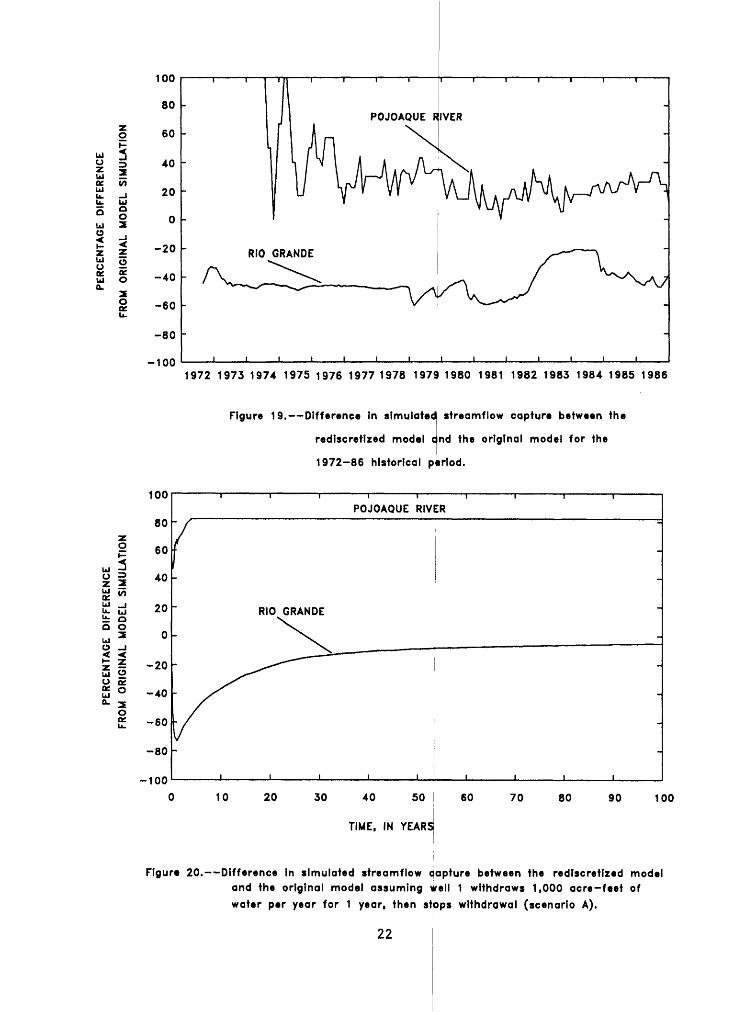
The model simulations for the 1972-86 historical period and the hypothetical withdrawals in scenarios A, B, C, and D were rerun using the rediscretized model. The differences in simulated streamflow capture between the rediscretized model and the original model are shown in figures 19 through 23.
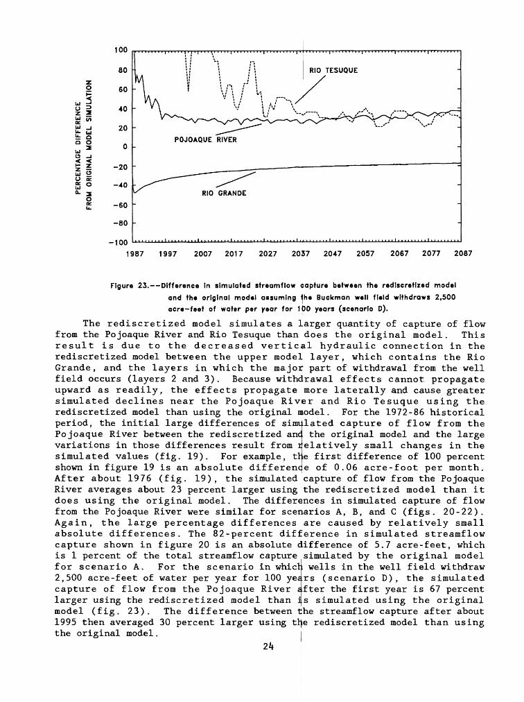
In general, the rediscretized model simulates a smaller quantity of capture of flow from the Rio Grande than does the original model. This result is due to the decreased vertical hydraulic connection in the rediscretized model between the Rio Grande and the model layers in which the major part of withdrawal from the well field occurs. For the 1972-86 historical period, the simulated capture of flow from the Rio Grande was 21 to 60 percent less using the rediscretized model than it was using the original model (fig. 19). For the scenario in which well 1 pumps 1,000 acre-feet of water per year for 1 year (scenario A), the simulated capture of flow from the Rio Grande after 1 year was 73 percent less using the rediscretized model than that using the original model (fig. 20). The percentage difference between the streamflow capture simulated by the two models then decreased with time to less than 20 percent after 21 years. For the scenarios in which well 2 (scenario B) and wells 3, 4, 5, and 6 (scenario C) respectively pump 1,000 acre-feet of water per year for 1 year, the percentage differences between the simulated streamflow capture using the rediscretized and the original models were similar (figs. 21 and 22). For these two sets of scenarios, simulated capture of flow from the Rio Grande was initially larger using the rediscretized model than it was using the original model but later decreased to more than 20 percent less than in the original model. After 10 years for scenario B and 16 years for scenario C, capture of flow from the Rio Grande was within 20 percent of that simulated by the original model . For the scenario in which the well field is assumed to withdraw 2,500 acre-feet of water per year for 100 years (scenario D), the simulated capture of flow from the Rio Grande after the first year was 48 percent less using the rediscretized model than it was using the original simulation (fig. 23). The difference in streamflow capture simulated by the two models then decreased to less than 20 percent by 2049.
21
PE
RC
EN
TAG
E
DIF
FE
RE
NC
E
FRO
M
OR
IGIN
AL
M
OD
EL
S
IMU
LA
TIO
N
PE
RC
EN
TAG
E
DIF
FE
RE
NC
E
FRO
M
OR
IGIN
AL
M
OD
EL
SIM
UL
AT
ION
ro
p*J I o
3
5
»
O
-c
2.
3«
<0
0
5*
« o
3-»
. c
°
o I
~*
Q.
Q.
O
O
1-0
^O
Q
c
3
?
§.=
:5
3
O
-C n 3D
i-l
fi*
8
--
»
O
°
D
?
o
5?^ 3
"
i
£S
S5-
o.
2. 3 o a
<o -si ro I a
<n
I 1 o
3.
O a.o.
2. i
3"
Q
* 3
o
*a
o<a
<
1 2
l! 2-
cr-*
2.
2 <

100
40 50
TIME, IN YEARS
60 70 80 90 100
O =>
.
5° o o
liLJ CD
«1uj O
Figure 21. Difference in simulated streamflow capture between the redlscretized model
and the original model assuming well 2 withdraws 1,000 acre-feet of
water per year for 1 year, then stops withdrawal (scenario B).
100
10 20 30 40 50
TIME, IN YEARS
60 70 80 90 100
Figure 22. Difference in simulated streamflow capture between the rediscretlzed model and the original model assuming wells 3, 4, 5, and 6 withdraw a total of 1,000 acre-feet of water per year for 1 year, then stop withdrawal
(scenario C).
b o0 O
O Ka- OUi
100
80
60
40
20
0
-20
-40
-60
-80
-100
POJOAQUE RIVER
RIO GRANDE
1987 1997 2007 2017 2027 2037 2047 2057 2067 2077 2087
Figure 23. Difference in simulated streamflow capture between the rediscretized model
and th« original model assuming th« Buckman w«ll fi«ld withdraws 2,500
ocr«-feet of water per year for 100 years (scenario D).
The rediscretized model simulates a larger quantity of capture of flow from the Pojoaque River and Rio Tesuque than does the original model. This result is due to the decreased vertical hydraulic connection in the rediscretized model between the upper model layer, which contains the Rio Grande, and the layers in which the majoi[ part of withdrawal from the well field occurs (layers 2 and 3). Because withdrawal effects cannot, propagate upward as readily, the effects propagate more laterally and cause greater simulated declines near the Pojoaque River and Rio Tesuque using the rediscretized model than using the original model. For the 1972-86 historical period, the initial large differences of simulated capture of flow from the Pojoaque River between the rediscretized and. the original model and the large variations in those differences result from relatively small changes in the simulated values (fig. 19). For example, the first difference of 100 percent shown in figure 19 is an absolute difference of 0.06 acre-foot per month. After about 1976 (fig. 19), the simulated capture of flow from the Pojoaque River averages about 23 percent larger using the rediscretized model than it does using the original model. The differences in simulated capture of flow from the Pojoaque River were similar for scenarios A, B, and C (figs. 20-22). Again, the large percentage differences are caused by relatively small absolute differences. The 82-percent difference in simulated streamflow capture shown in figure 20 is an absolute difference of 5.7 acre-feet, which is 1 percent of the total streamflow capture simulated by the original model for scenario A. For the scenario in which wells in the well field withdraw 2,500 acre-feet of water per year for 100 yes.rs (scenario D) , the simulated capture of flow from the Pojoaque River s.fter the first year is 67 percent larger using the rediscretized model than is simulated using the original model (fig. 23). The difference between the streamflow capture after about 1995 then averaged 30 percent larger using ttye rediscretized model than using the original model.
24
The initial large differences in simulated capture of flow from the Rio Tesuque between the rediscretized model and the original model for scenario D, as well as the large fluctuations in those differences (fig. 23), are the result of relatively small changes in the absolute values, as was the case for the Pojoaque River. The first difference of 100 percent shown in figure 23 is an absolute difference of 1 acre-foot per year. After about 50 years in the simulation (about 2037), the capture of flow from the Rio Tesuque simulated by the rediscretized model averaged 31 percent larger than that simulated by the original model.
The sensitivity analysis shows that the simulated streamflow capture is sensitive to the changes made to the original model. In particular, the simulated streamflow capture seems to be sensitive to changes in the layering of the model and, therefore, would be sensitive to modeled changes of vertical hydraulic conductivity.
The rediscretized model used in this sensitivity analysis is not a calibrated model. A calibrated model designed specifically for the objectives of this study will not produce the same results as the rediscretized model used in this analysis. The magnitudes of the differences between simulated streamflow capture by using such a calibrated model and the Santa Fe area model would not be as large as the differences shown in this analysis. However, such a calibrated model should simulate results showing similar trends; that is, it should simulate less capture of flow from the Rio Grande and more from the Pojoaque River and Rio Tesuque than does the Santa Fe area model as a result of Buckman well-field withdrawal.
SUMMARY
The digital three-dimensional ground-water flow model developed for the Santa Fe area by McAda and Wasiolek (1988) was used to demonstrate the use of a basinwide model to evaluate the effects of ground-water withdrawal from wells on flow in nearby rivers. Model simulations of ground-water withdrawal from the Buckman well field were made in order to estimate the magnitude of effects of withdrawal on flow in the Rio Grande, Pojoaque River, and Rio Tesuque. A simulation of historical withdrawal from the well field from 1972 through 1986 resulted in an estimated streamflow capture for the same time period of 8,450 acre-feet (36 percent of withdrawal) from the Rio Grande and 112 acre-feet (0.5 percent of withdrawal) from the Pojoaque River.
A series of model simulations that used hypothetical withdrawals from specific wells in the Buckman well field was used to illustrate the effects of withdrawal from those wells on the rivers. From the simulation in which well 1 pumped 1,000 acre-feet of water per year for 1 year, 65 percent of the total withdrawal was captured from the Rio Grande after 20 years and 0.78 percent of the withdrawal was captured from the Pojoaque River after 2.4 years. From the simulation in which well 2 pumped 1,000 acre-feet of water per year for 1 year, 49 percent of the total withdrawal was captured from the Rio Grande after 36 years and 0.75 percent of the withdrawal was captured from the Pojoaque River after 2.4 years. From the simulation in which wells 3, 4, 5, and 6 pumped 1,000 acre-feet of water per year for 1 year, 41 percent of the
25
total withdrawal was captured from the Rio Grande after 32 years and 0.81 percent of the withdrawal was captured from the Pojoaque River after 3 years. From the simulation in which well 1 pumped 12,000 acre-feet of water per year for 1 year, 67 percent of the withdrawal was captured from the Rio Grande after 29 years and 0.39 percent of the withdrawal was captured from the Pojoaque River after 3 years. From the simulation in which well 2 pumped 2,000 acre-feet of water per year for 1 year,, 54 percent of the withdrawal was captured from the Rio Grande after 43 years a|nd 0.36 percent of the withdrawal was captured from the Pojoaque River after 2.4 years. From the simulation in which wells 3, 4, 5, and 6 pumped 2,000 4cre-feet of water per year for 1 year, 46 percent of the withdrawal was captured from the Rio Grande after 47 years and 0.39 percent of the withdrawal was captured from the Pojoaque River after 2.4 years. From the simulation in which wells 1 and 2 together pumped 2,500 acre-feet of water per year continuously, the simulated annual streamflow capture after 100 years, as a percentage of annual withdrawal by the wells, was 74 percent from the Rio Grand^, 2.8 percent from the Pojoaque River, and 1.2 percent from the Rio Tesuque. From the simulation in which wells 1 and 2 together pumped 5,000 acre-feet of water per year continuously, the simulated annual streamflow capture after 100 years, as a percentage of annual withdrawal by the wells, was 74 percent from the Rio Grande, 2.9 percent from the Pojoaque River, and 1.3 percent from the Rio Tesuque.
Two simulations were made using the projected withdrawal from the Buckman well field from 1987 to 2045 as reported oy the Santa Fe Metropolitan Water Board (1984, table 4-2) for the projected small and large water demands of Santa Fe . At the end of the simulation using the small water demand, projected withdrawal from the Buckman well field was 3,860 acre-feet per year, and the simulated streamflow capture was 2,3^0 acre-feet per year from the Rio Grande, 49 acre-feet per year from the Pojoaque River, and 11 acre-feet per year from the Rio Tesuque. At the end of the simulation using the large water demand, projected withdrawal from the Buckman well field was 6,660 acre-feet per year, and the simulated streamflow capture was 4,260 acre-feet per year from the Rio Grande, 99 acre-feet per year from the Pojoaque River, and 28 acre-feet per year from the Rio Tesuque.
The sensitivity of the simulated effect^ of withdrawal from the Buckman well field on streamflow to the discretisation of the model was tested by comparing the results from the original model simulations with the results from a rediscretized model. The rediscretized model was created by refining the original model grid in the area representing the Buckman well field and dividing each of the upper two model layers Into two layers. This sensitivity analysis showed that the simulated streamflow capture is sensitive to those changes.
26
REFERENCES
Baltz, E.H., 1978, Resume of the Rio Grande depression in north-central New Mexico, in Guidebook to Rio Grande rift in New Mexico and Colorado: New Mexico Bureau of Mines and Mineral Resources Circular 163, p. 210-228.
Galusha, Ted, and Blick, J.C., 1971, Stratigraphy of the Santa Fe Group, New Mexico: American Museum of Natural History Bulletin, v. 144, article 1, p. 1-127.
Griggs, R.L., 1964, Geology and ground-water resources of the Los Alamos area, New Mexico: U.S. Geological Survey Water-Supply Paper 1753, 107 p., 1 pi.
Kelley, V.C., 1978, Geology of Espanola Basin, New Mexico: New Mexico Bureau of Mines and Mineral Resources Geologic Map 48, scale 1:125,000.
Manley, Kirn, 1978a, Structure and stratigraphy of the Espanola Basin, Rio Grande rift, New Mexico: U.S. Geological Survey Open-File Report 78-667, 24 p.
____1978b, Cenozoic geology of Espanola Basin, in Guidebook to Rio Grande rift in New Mexico and Colorado: New Mexico Bureau of Mines and Mineral Resources Circular 163, p. 201-210.
McAda, D.P., and Wasiolek, Maryann, 1988, Simulation of the regional geohydrology of the Tesuque aquifer system near Santa Fe, New Mexico: U.S. Geological Survey Water-Resources Investigations Report 87-4056, 71 p.
McDonald, M.G., and Harbaugh, A.W., 1988, A modular three-dimensional finite- difference ground-water flow model: U.S. Geological Survey Techniques of Water-Resources Investigations, Book 6, Chap. Al, various pagination.
Purtymun, W.D., and Johansen, Steven, 1974, General geohydrology of the Pajarito Plateau, in Guidebook to Ghost Ranch (central-northern New Mexico): New Mexico Geological Society, 25th Field Conference, p. 347- 349.
Santa Fe Metropolitan Water Board, 1984, Santa Fe regional water supply system--Report on baseline data, goals, policy and studies: Santa Fe Metropolitan Water Board publication, various pagination.
Spiegel, Zane, and Baldwin, Brewster, 1963, Geology and water resources of the Santa Fe area, New Mexico: U.S. Geological Survey Water-Supply Paper 1525, 258 p.
27