simulation of transient flows in a hydraulic …ptmts.org/zarzycki-4-07.pdf · journaloftheoretical...

JOURNAL OF THEORETICAL

AND APPLIED MECHANICS

45, 4, pp. 853-871, Warsaw 2007

SIMULATION OF TRANSIENT FLOWS IN A HYDRAULIC

SYSTEM WITH A LONG LIQUID LINE

Zbigniew Zarzycki

Sylwester Kudźma

Szczecin University of Technology, Department of Mechanics and Machine Elements, Poland

e-mail: [email protected]; [email protected]

Zygmunt Kudźma

Michał Stosiak

Wrocław University of Technology, Institute of Machine Design and Operation, Poland

e-mail: [email protected], [email protected]

The paper presents the problem of modelling and simulation of transientsphenomena in hydraulic systems with long liquid lines. The unsteadyresistance model is used to describe the unsteady liquid pipe flow. Thewall shear stress at the pipe wall is expressed by means of the convolutionof acceleration and a weighting function which depends on the (laminaror turbulent) character of the flow. The results of numerical simulationare presented for the waterhammer effect, which is caused by a suddenshift of the hydraulic directional control valve. The following cases of thesystem supply are considered: the first, with a constant delivery rate ofthe pump and the second, which additionally considers pulsation of thedelivery of the pump. Computer simulations are compared with resultsof experiments. They are found to be very consistent in the case withthe variable rate of the pump delivery taken into accent.

Key words: unsteady pipe flow, transients, waterhammer, pulsation ofpump

1. Introduction

Drive and hydraulic control systems are often subjected to transient states,caused by dynamical excitation forces resulting either from sudden changesof the load of a motor or hydraulic actuator or else from changes of the flow

854 Z. Zarzycki et al.

direction of the working liquid or speed caused by the control unit. It is oftenessential to precisely learn characteristics of dynamical runs in such states.It is very important in the design of automatic control systems or in the foranalyzis of the strength of pipes and other elements of hydraulic systems.

While analyzing transient states, particular attention should be paid tosuch cases when a hydraulic system has a long liquid line (Garbacik and Szew-czyk, 1995; Wylie and Streeter, 1978; Jelali and Kroll 2003), i.e. either whenthe length of the pipe is close to that of the pressure wave which is propagatedin the system or when it is higher than that. Such a pipe is treated then as anelement of a system with distributed parameters. Consequently, any changesof the flow pressure and rate are distributed along the pipes axis with a limitedspeed in the form of progressive and reflected waves.

In literature, the research of transient states concern mostly simple water-hammer cases (Wylie and Streeter, 1978; Ohmi et al., 1985), in which simpleboundary conditions are used. It means that at one end of the hydraulic linethe pressure is constant (reservoir) and at the other, the velocity of flow equalszero (suddenly closed valve).

The present paper is an attempt at simulating transients caused by a sud-den change of settings of the hydraulic control valve, with taking into accountat the same time the pulsation delivery rate resulting from kinematics of apositive-displacement pump. The results obtained from numerical simulationsare compared and validated with the recorded runs of pressure changes on aspecially built test stand.

2. Mathematical model of the flow

The aim of the present paper is to present simulations of pressure transientsof the considered system in cases of sudden jumps of pressure at the end of along hydraulic line caused by e.g. operational overload.

The fundamental component of the hydraulic system, shown in Fig. 1, isthe liquid long line which is treated as a distributed parameter element. Thesystem is a subassembly, which is often found in many hydraulic systems oftechnical machinery and devices used e.g. in mining or ship building industry.

2.1. Fundamental equations

The unsteady flow in liquid pipes is often represented by two 1D hyper-bolic partial differential equations. Linearized equations of momentum and

Simulation of transient flows in a hydraulic system... 855

Fig. 1. The object of investigations

continuity can be given by Jungowski (1976), Ohmi et al. (1985) and Zarzycki(1994)

ρ0∂v

∂t+∂p

∂z+2

Rτw = 0

∂p

∂t+ ρ0c

20

∂v

∂z= 0 (2.1)

where: t is time, z – distance along the pipe axis, v = v(z, t) – average valueof velocity in a cross-section of the pipe, p = p(z, t) – average value of pressurein a cross-section of pipe, τw – shear stress in the pipe wall, ρ0 – density ofthe liquid (constant), R – inner radius of the pipe.The speed of the acoustic wave c0 in Eq. (2.1)2 takes into consideration

compressibility of the liquid and elastic deformability of the pipe wall, and canbe given by the following relation (Wylie and Streeter, 1978)

c0 =

√βcρc

1√1 + 2βc

ERg

(2.2)

where βc is the bulk modulus of the liquid, E – Young’s modulus of the tubeand g – thickness of the wall.In an unsteady flow in the pipe, the instantaneous stress τw may be re-

garded as a sum of two components: the quasi-steady state shear componentand the unsteady state shear component (Ohmi et al., 1985; Zarzycki, 2000)

τw =1

8λρ0v|v|+

2µ

R

t∫

0

w(t− u)∂v∂t(u) du (2.3)

where: λ is the Darcy-Weisbach friction coefficient, w – weighting function,µ – dynamic viscosity, u – time used in the convolution integral.The first component in Eq. (2.3) presents the quasi-steady state of the wall

shear stress, the second one is the additional contribution due to unsteadiness.


The second summand in Eq. (2.3) relates the wall shear stress to the instanta-neous average velocity and to the weighted past velocity changes. The systemof Eqs. (2.1) and (2.3) is closed because of p and v, as long as the weightingfunction w(t) is known for the wall shear stress at the pipe wall.

2.2. Weighting functions

Zielke (1968) was first to give an analytical relation for the weighting func-tion w(t) for a laminar flow. He derived it from the analysis of a transienttwo-dimensional laminar flow. The Zielke model can be given by

w(t) =

6∑

i=1

miti−2

2 for t ¬ 0.025∑

i=1

exp(−nit) for t > 0.02

(2.4)

where mi is 0.28209, −1.25, 1.05778, 0.93750, 0.396696, −0.351563 andni = −26.3744, −70.8493, −135.0198, −218.9216, −322.5544, respectively,and t is the dimensionless time, defined by the following relation

t = νt

R2(2.5)

Zielke’s model requires much computer memory and, therefore, it was modifiedby Trikha (1975) and Schoohl (1993) to improve its computational efficiency.

Schoohl’s model can be given by

w(t) =5∑

i=1

mi exp(−nit) (2.6)

where: m1 = 1.051, m2 = 2.358, m3 = 9.021, m4 = 29.47, m5 = 79.55,n1 = 26.65, n2 = 100, n3 = 669.6, n4 = 6497, n5 = 57990.

In the case of the unsteady turbulent flow, the weighting function dependsnot only on the dimensional time but also on the Reynolds number. Vardy etal. (1993) and Vardy and Brown (1996) derived a model in which all viscosityeffects were assumed to occur in the steady boundary layer (viscosity variedlinearly across the outer annular shear layer). An approximated form of theirweighting function model is

wa =1

2√πtexp(− tC∗

)(2.7)


where

C∗ = 12.86Rek

k = log1015.29

Re0.0567

Zarzycki (1994, 2000) developed a weighting function model using a four-region discretization (four instead of two regions) for turbulent viscosity di-stribution. The model had a complex mathematical form and it was furtherapproximated to a simpler form

wapr = C1√tRen (2.8)

where: C = 0.299635, n = −0.005535.Zarzycki’s model yields the same results as Vardy’s model, but generates

them more quickly. In Eq. (2.8), both time and Reynold’s number (i.e. also thespeed) are in the denominator, which makes calculations difficult. In order toeliminate these difficulties, Zarzycki and Kudźma (2004) and Kudźma (2005)presented a model similar to Schohl’s model for a laminar flow. Their modelcan be given by

wN (t) = (c1Rec2 + c3)

6∑

i=1

Ai exp(−bit) (2.9)

where: A1 = 152.3936, A2 = 414.8145, A3 = 328.2, A4 = 640.2165,A5 = 58.51351, A6 = 17.10735, b1 = 207569.7, b2 = 6316096, b3 = 1464649,b4 = 15512625, b5 = 17790.69, b6 = 477.887, c1 = −1, 5125, c2 = 0.003264,c3 = 2.55888.The value of critical Reynold’s number (between unsteady laminar and

turbulent flow), which qualifies the application of an appropriate weightingfunction, can be calculated by means of the following empirical relation (Ohmiet al., 1985)

Recn = 800√Ω (2.10)

Equation (2.10) can be used for an oscillatory flow, whereas for a pulsatingflow Recn is (Ramaprian and Tu, 1980)

Recn = 2100 (2.11)

where: Ω = ωR2/ν denotes the dimensionless frequency, ω = 2π/T – dimen-sional frequency, T = 4L/c0 – period of the waterhammer, L – length of thepipe.For further simulations of the hydraulic waterhammer effect, two models

were adopted: model (2.6) for the laminar flow and model (2.9) for the turbu-lent flow.


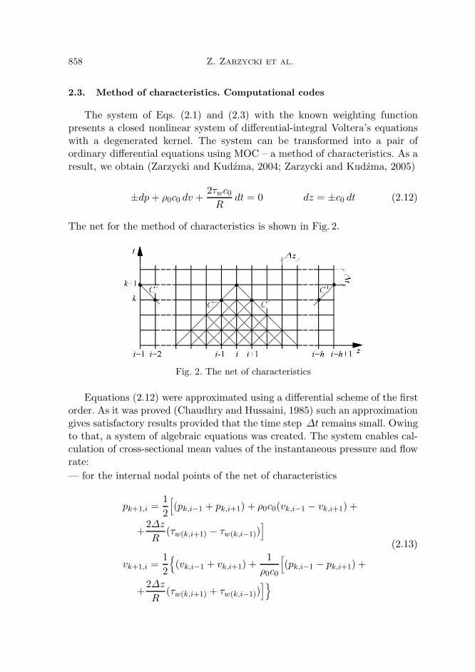
2.3. Method of characteristics. Computational codes

The system of Eqs. (2.1) and (2.3) with the known weighting functionpresents a closed nonlinear system of differential-integral Voltera’s equationswith a degenerated kernel. The system can be transformed into a pair ofordinary differential equations using MOC – a method of characteristics. As aresult, we obtain (Zarzycki and Kudźma, 2004; Zarzycki and Kudźma, 2005)

±dp+ ρ0c0 dv +2τwc0Rdt = 0 dz = ±c0 dt (2.12)

The net for the method of characteristics is shown in Fig. 2.

Fig. 2. The net of characteristics

Equations (2.12) were approximated using a differential scheme of the firstorder. As it was proved (Chaudhry and Hussaini, 1985) such an approximationgives satisfactory results provided that the time step ∆t remains small. Owingto that, a system of algebraic equations was created. The system enables cal-culation of cross-sectional mean values of the instantaneous pressure and flowrate:

— for the internal nodal points of the net of characteristics

pk+1,i =1

2

[(pk,i−1 + pk,i+1) + ρ0c0(vk,i−1 − vk,i+1) +

+2∆z

R(τw(k,i+1) − τw(k,i−1))

]

(2.13)

vk+1,i =1

2

(vk,i−1 + vk,i+1) +

1

ρ0c0

[(pk,i−1 − pk,i+1) +

+2∆z

R(τw(k,i+1) + τw(k,i−1))

]


— for the boundary nodal points of the net of characteristics:

pk+1,1 = pk,2 + ρ0c0[(vk+1,1 − vk,2) +

2∆t

Rτw(k,2)

]

(2.14)

vk+1,h+1 = vk,h +1

ρ0c0(pk,h − pk+1,h+1)−

2∆t

Rτw(k,h)

where i = 2, 3, . . . , h, k = 1, 2, . . . ,m, m is the number of time steps, h –number of calculation sections along the hydraulic line.

As it was mentioned in Section 2.1, the instantaneous shear stress τw canbe given by a sum of two components

τw(k,i) = τwq(k,i) + τwn(k,i) (2.15)

where

τwq(k,i) =1

8ρ0λ(Rek,i)vk,i|vk,i|

(2.16)

τwn(k,i) =2µ

R[(vk,i − vk−1,i)w1,i + (vk−1,i − vk−2,i)w2,i + . . .+

+(v2,i − v1,i)wk−1,i]

The friction loss coefficient λ in Eq. (2.16)1 is expressed for the laminar flowby

λ =64

Re(2.17)

And for the turbulent flow, from Prandtl’s formula, by

1√λ= 0.869 ln(Re

√λ)− 0.8 (2.18)

The system of Eqs. (2.13)-(2.18) together with Eqs. (2.6), (2.9) and the boun-dary and initial conditions is the basis for creating an algorithm of calculationsand then a computer program.

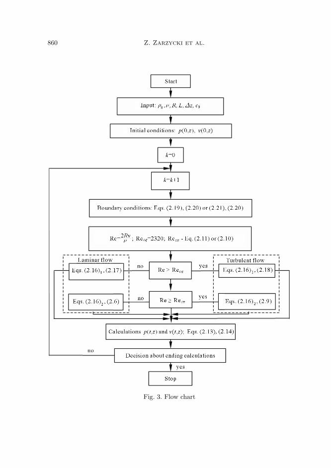
Figure 3 presents the algorithm of calculations.

2.4. Verification of the model

In order to compare the accuracy of unsteady and quasi-steady models offriction in relation to experimental data, simulations of a simple waterhammercase (tank – long liquid line and cut-off valve) were conducted.


Fig. 3. Flow chart


The computed results were compared with experimental data reported byHolmboe and Rouleau (1967). They ran tests on a copper tube with radius0.0127m and length 36.1 m connected upstream to a tank which was main-tained at a constant pressure by the compressed air. The liquid used in theexperiment was an oil having viscosity 39.7 · 10−6m2/s. The measured soundspeed was 1324m/s and the initial flow velocity 0.128m/s (Re = 82). Thedownstream valve was rapidly closed in the pipe line during flow. Pressurefluctuation was measured at the midpoint of the line. From the above para-meters, it followed that it was a case of a laminar flow. It was determined innumerical calculations in which the models of Zielke, Eq. (2.4), and Schoohla(2.6) were used. In addition, the calculation with the quasi-steady model onlyi.e., with Eqs. (2.16)1 and (2.17) was done as well.Results of simulations and experimental data are shown in Fig. 4. It is

clearly seen that the calculation using the weighting functions (changeablehydraulic resistance) is much closer to the experimental data. Therefore, infurther calculations the weighting functions were used instead of the quasi-steady model.

Fig. 4. Fluctuations of pressure at the midpoint of the line; 1 – experimental data,2 – simulations with the unsteady model of friction, 3 – simulations with the

quasi-steady model

2.5. Boundary conditions

It is necessary to know boundary conditions in order to be able to solve thesystem of Eqs. (2.1) and (2.4) using the method of characteristics. The analysisinvolves pressure runs at the beginning and at the end of the long line (Fig. 1)during a sudden shift of the hydraulic directional control valve in time t0.


At that moment, a sudden change in the pressure from p0 to p0 +∆p takesplace. Two cases are investigated. The first case assumes a constant rate ofdelivery of the positive-displacement pump, the second one takes into accountpulsation of the delivery of the pump. These conditions can be expressed inthe following way:

— for a constant rate of delivery for z = 0

Q(t) = const (2.19)

and for z = L

p =

p0 for 0 ¬ t < t0p0 +∆p for t t0

(2.20)

— for a changeable rate of delivery for z = 0

Q = Qm[1− 12

K=∞∑

K=1

δQK cos(ωKt)]

(2.21)

where: ωK denotes pulsations of harmonic vibration of the pump, K – orderof harmonics, δQK – relative amplitudes of harmonic vibration of the flowrate according to the literature data, Qm – mean theoretical efficiency.

Relation (2.21) was obtained by Rohatynski (1968). The condition forz = L has the form expressed in Eq. (2.20).

3. The test stand and description of experimental investigations

In order to validate the presented model and the method for simulation ofthe hydraulic waterhammer effect, some tests were carried out on a speciallyprepared test stand. A diagram of the hydraulic system of the test stand ispresented in Fig. 5. The central part of the system comprised a hydraulic li-ne. Two extensometer pressure converters (7), (9) of the working liquid werefixed to its two ends. The generated flow intensity through the axial-flow mul-tipiston pump with deflected disc (6) Z-PTOZ2-K1-100R1 was measured byflowmeter (13). At the end of the hydraulic line, hydraulic control valve (10)(4/2) was installed, whose function was to suddenly direct the liquid throughthrottle valve (11). In order to realises an increase in the system load an adju-stable throttle valve was used. To protect the system against an incidental anddangerous pressure increase, safety valve (8) was installed right at the pump.


Fig. 5. A scheme of the hydraulic system used in experimental investigations on thepressure wave velocity propagation: 1 – hydraulic constant delivery pump (pressurecharging pump), 2 – safety valve, 3 – filter, 4 – throttle valve, 5 – vacuometer,

6 – hydraulic variable displacement pump, 7 – pressure transducer, 8 – safety valve,9 – pressure transducer, 10 – directional control valve 4/2, 11 – throttle valve,12 – check valve, 13 – flowmeter, 14 – water cooler, 15 – thermometer

The unsteady state in the system was caused by the shifted hydraulicdirectional control valve directing the liquid flow through the throttle valvewith higher hydraulic resistance d2 (Fig. 1).

The time of shift of the directional control valve was tz = 20ms. It wasshorter than half of the hydraulic hammer time (tz < T/2 = 2L/c0 = 0.028 s,L = 18m, c0 = 1309m/s which is determined in a further part of thispaper).

The recording of the instantaneous pressure series at some points of thehydraulic line was carried out by means of measuring equipment consistingof tensometric pressure sensors, screened conductors eliminating the outsi-de interference, digital oscilloscope Tektronix TDS-224, multi-channel signalamplifier TDA-6, computer with an analogue-digital card AD/DA and WaveStar-Tektronix software.

4. Spectroscopic analysis of pressure pulsation in the steady state

The recording of the pressure series in a steady state (before the shift of thedirectional control valve) was carried out in two measuring points: behind the


pump and in front of the control valve. The recorded time series are presen-ted in Fig. 6. They display pressure pulsation resulting from the operation ofthe positive-displacement pump. The dominant pulsation frequency for theinvestigated system can be estimated from the following relation

fK =npzK

60[Hz] (4.1)

where np is the speed of rotation of the pump shaft [rev/min], z – number ofdisplacement elements, K – number of harmonics, K = 1, . . . , n.The investigated system comprised an axial-flow multi-piston pump with a

deflected disk of the type PTOZ-100 driven at the speed n = 1500 rev/min andcontaining z = 9 pistons, which according to relation (4.1) yields f1 = 225Hz.

Fig. 6. The recorded time series during steady operation of the system. Data:ν = 100 cSt, mean pressure at the valve p0 = 1.2MPa, mean intensity of the flow

Q = 50dm3/min

Additionally, on the basis of the time series, an FFT spectroscopic analy-sis of the pressure pulsation was carried out. Figure 7 presents the obtainedresults.As it can be seen in the presented diagrams of pressure pulsation spectra,

the dominant frequency in the analyzed series is the operational frequency ofthe positive-displacement pump. The first frequency f1 is 225Hz. The suc-cessive harmonics are respectively f2 = 450Hz, f3 = 675Hz, f4 = 900Hz,...The analysis carried out during the investigations makes it possible to take

into account the first harmonic in boundary condition (2.21), the harmonicresulting from kinematics of the pump. Higher frequencies require a much finernumerical grid, which very significantly decrease the efficiency of simulation(in our tests time of calculations was prolonged hundred times).


Fig. 7. Amplitude-frequency spectra of the pressure pulsation in the hydraulicsystem caused by the non-uniform delivery of the pump

5. Numerical and experimental results

As it was mentioned earlier, the series of pressure changes were investigatedafter a sudden shift of the control valve at measuring point 1 (at the controlvalve) and point 2 (at the pump).

The parameters of the line were as follows: length of the line L = 18m,inner diameter of the line d = 2R = 9mm, thickness of the line wallg = 1.5mm, material of the line steel E = 2.1 · 1011 Pa.The working liquid of the system was a hydraulic oil (HL 68) with density

ρ0 = 860 kg/m3 and the modulus of volume elasticity βc = 1.5 · 109 Pa.

The speed of sound c0 calculated according to Eq. (2.2) was 1309m/s.

The investigations were carried out for two variants:

• laminar flow: Re = 471 (ν = 150 cSt)• turbulent flow: Re = 2829 (ν = 50 cSt)

In both variants, the delivery rate of the pump in the boundary conditioncould either be constant (Eq. (2.19)) or changeable (Eq. (2.21)).

The simulation investigations were carried out according to the algori-thm presented in Fig. 3. The adopted number of the measured segments wash = 20, the length of the calculated segment ∆z = L/h = 0.9m and the valueof the time step ∆t = ∆z/c0 = 0.007 s.

Figures 8-11, shown below, present both the recorded series and the expec-ted series simulated numerically. In Figs. 7-10, numbers 1-4 correspond to:

1 – numerical simulation, pressure at the hydraulic pump

2 – pressure at the valve (the boundary condition in calculations)

3 – experimental data, pressure at the hydraulic pump

4 – experimental data, pressure at the valve.


Fig. 8. Comparison between experimental and numerical results; ν = 150 cSt,Q = 30dm3/min, p0 = 0.7MPa, L = 18m, ∆p = 4.9MPa (Q – mean intensity of

the flow rate, p0 – mean pressure at the valve before unsteady state)

Fig. 9. Comparison between experimental and numerical results; ν = 50 cSt,Q = 60dm3/min, p0 = 1.85MPa, L = 18m, ∆p = 7.8MPa

Using the above mentioned boundary conditions, numerical simulation wascarried out. The obtained results were compared with those determined expe-rimentally and presented in Fig. 10 and Fig. 11.

The verification assessment of the numerical results with the experimentaldata is problematic due to interference recorded during the experiment. As itcan be seen in the comparisons presented in Figs. 8-11, the pressure pulsa-tion resulting from the irregular operation of the pump greatly influences therecorded experimental series.


Fig. 10. Comparison between experimental and numerical results for the transientstate with pulsating intensity of the liquid flow taken into account at the boundarycondition; ν = 150 cSt, Q = 30dm3/min, p0 = 0.7MPa, L = 18m, ∆p = 4.9MPa

Fig. 11. Comparison between experimental and numerical results for the transientstate with pulsating intensity of the liquid flow taken into account at the boundarycondition; ν = 50 cSt, Q = 60dm3/min, p0 = 1.85MPa, L = 18m, ∆p = 7.8MPa

We should not forget about other factors which may also influence theexperiment. These include:

• changes in the viscosity and density of the liquid along the line causedby temperature changes of the flowing liquid. It should be rememberedthat while flowing through the hydraulic line, the temperature of theliquid, owing to friction, goes up by even a dozen or so degrees. Thetemperature increase is connected with some changes in properties of


the liquid. In order to minimize the influence the temperature may haveon the results of the experiment, a water cooler was used

• the undissolved air found in the oil used in the hydraulic system maycause an interference and a time-lag of the phase series (Wylie and Stre-eter, 1978). In order to eliminate this interference, the exhaust line ofthe pump was equipped with the so-called supercharging pump, whichensured that in the exhaust area the pressure did not go below the pres-sure of air precipitation from the oil, which made it possible to avoidcavitation (Kollek et al., 2003).

• fluid structure interactions may also lead to interferences in pressurechanges

• the shift of the control valve directing the flow of the liquid through thethrottle valve with a higher hydraulic resistance does not fully reflect theabrupt (rectangular) pressure changes at the control valve. Additionalpressure oscillations appear as well (particularly at a high flow inten-sity and low viscosity). Most probably, they are due to very short butcomplete stoppage of the liquid flow during the shift of the control valve.

6. Concluding remarks

The following conclusions can be drawn from the tests that were carried outin this study:

• the application of the developed method for simulating transients whilealso taking into account unsteady friction resistance of the liquid (Eqs.(2.13)-(2.18) together with Eqs. (2.6) and (2.9)) provides a convenientmethod for effective numerical calculations for both laminar and turbu-lent flows

• in the registered pressure changes in the quasi-steady state, the pulsationof the delivery rate of the pump plays a significant role. It may causepressure pulsation up to ±10-20% of the mean pressure• in the investigations of transient states caused by load changes of thehydraulic system resulting from a sudden change in the flow and direc-ting it through the throttle valve with a higher hydraulic resistance, thepressure pulsation which results from the delivery pulsation significantlyinterferes and distorts the pressure changes


• if the pulsation of the hydraulic pump delivery is taken into account inthe boundary conditions, it significantly brings the results of numericalsimulations closer to the experimental data.

Notation

c0 – acoustic wave speed, [m/s]E – Young’s modulus, [N/m2]g – thickness of wall pipe, [m]f – frequency of the pulsation, [s−1]L – pipe length, [m]m – number of time steps, [–]np – speed of rotation, [rpm]p – pressure, [Pa]R – radius of pipe, [m]Re,Recn – Reynolds number and critical Reynolds number, respec-

tively, [–]T – period of waterhammer, [s]t – time, [s]

t = νt/R2 – dimensionless time, [–]v – instantaneous mean flow velocity in the cross section,

[m/s]w – weighting function, [–]z – distance along pipe axis, [m]βc – bulk modulus of the liquid, [Pa]λ – Darcy-Weisbach friction coefficient, [–]µ – dynamic viscosity, [kgm−1s−1]ν – kinematic viscosity, [m2s−1]ρ0 – fluid density (constant), [kgm−3]τw, τwq, τwu – wall shear stress, wall shear stress for quasi-steady flow

and unsteady wall shear stress, respectively, [kgm−1s−2]ω – angular frequency of the pulsation, [s−1]Ω = ωR2/ν – dimensionless frequency, [–]

References

1. Chaudhry M.H., Hussaini M.Y., 1985, Second-order explicit finite-differenceschemes for waterhammer analysis, Journal of Fluids Engineering, 107, 523-529


2. Garbacik A., Szewczyk K., 1995, New Aspects of Modelling of Fluid PowerControl, Wrocław, Warszawa, Kraków, Ossolineum

3. Holmboe E.L., Rouleau W.T., 1967, The effect of viscous shear on transietsin liquid lines, Transactions ASME, Journnal of Basic Engineering, 89, 11,174-180

4. Jelali M., Kroll A., 2003, Hydraulic Servo-systems. Modelling, Identifica-tion and Control, Springer-Verlag, London

5. Jungowski W., 1976, One-dimensional Transient Flow, Publishing House ofWarsaw University of Technology [in Polish]

6. Kollek W., Kudźma Z., Stosiak M., 2003, Acoustic diagnostic testing inidentification of phenomena associated with flow of working medium in hydrau-lic systems [in Polish], Twelve Power Seminar ’2003 on Current Flow, Designand Operational Problems of Hydraulic Machines and Equipment, Gliwice, Po-land

7. Kudźma S., 2005, Modeling and simulation dynamical runs in closed conduitsof hydraulics systems using unsteady friction model, PhD work at SzczecinUniversity of Technology, February [in Polish]

8. Ohmi M., Kyonen S., Usui T., 1985, Numerical analysis of transient turbu-lent flow in a liquid line, Bulletin of JSME, 28, 239, 799-806

9. Ramaprian B.R., Tu S.-W., 1980, An experimental study of oscillatory pipeflow at transitional Reynolds number, J. Fluid Mech., 100, 3, 513-544

10. Rohatyński R., 1968, Damping of Pressure Pulsations in Hydraulic Systemswith Displacement Pumps, Scientific Work of Wroclaw University of Technology,No. 191, Power Engineering IX [in Polish]

11. Schohl G.A., 1993, Improved approximate method for simulating frequency-dependent friction in transient laminar flow, Journal of Fluids Eng., Trans.ASME, 115, 420-424

12. Trikha A. K., 1975, An efficient method for simulating frequency-dependentfriction in transient liquid flow, Journal of Fluids Eng., Trans. ASME, 97-105

13. Vardy A.E., Brown J., 1996, On turbulent, unsteady, smooth-pipe friction,Proc. of 7th International Conference on Pressure Surges, Harrogate UK, 16-18,BHRA Fluid Eng., 289-311

14. Vardy A.E., Brown J.M.B., Kuo-Lun H., 1993, A weighting function mo-del of transient turbulent pipe flow, J. Hyd. Res., 31, 4, 533-548

15. Wylie E.B., Streeter V.L., 1978, Fluid Transients, McGraw-Hill, New York

16. Zarzycki Z., 1994, A Hydraulic Resistances of Unsteady Lquid Flow in Pipes,Scientific Works at Szczecin University of Technology, No. 516, Szczecin


17. Zarzycki Z., 2000, On weighting function for wall shear stress during unsteadyturbulent pipe flow, 8th International Conference on Pressure Surges, BHRGroup, The Hague, 529-543

18. Zarzycki Z., Kudźma S., 2004, Simulations of transient turbulent flow inliquid lines using time-dependent frictional losses, The 9th International Con-ference on Pressure Surges, BHR Group, Chester, UK, 24/26, 439-455

19. Zarzycki Z., Kudźma S., 2005, Computation of transient turbulent flow ofliquid in pipe using unsteady friction formula, Transactions of the Institute ofFluid – Flow Machinery, 116, 27-42

20. Zielke W., 1968, Frequency-dependent friction in transient pipe flow, Journalof Basic Eng., Trans. ASME, 109-115

Symulacja przepływów przejściowych w układzie hydraulicznym

z hydrauliczną linią długą

Streszczenie

Artykuł przedstawia zagadnienie modelowania i symulacji zjawisk przejściowychw układach hydraulicznych z hydrauliczną linią długą. Wykorzystano model tarcianiestacjonarnego do opisu niestacjonarnego przepływu w przewodzie. Naprężenia ści-nające na ściankach przewodów są określone za pomocą przyspieszenia i finkcji wagi,która zależy od charakteru przepływu (uwarstwiony, turbulentny). Rezultaty symu-lacji numerycznych są prezentowane dla uderzenia hydraulicznego, które spowodowa-ne jest poprzez nagłe przesterowanie rozdzielacza. Rozpatrywane są dwa przypadki:pierwszy – gdy układ zasilający podaje stałą wartość natężenia przepływu, drugi –uwzględniający pulsację wydajności pompy wyporowej. Symulacje komputerowe sąporównane z wynikami badań eksperymentalnych. Wykazano dużą zgodność symu-lacji komputerowych uwzględniających pulsację wydajności pompy z wynikami eks-perymentu.

Manuscript received March 9, 2007; accepted for print April 25, 2007

simulation of transient flows in a hydraulic …ptmts.org/zarzycki-4-07.pdf · journaloftheoretical...

Documents