Simulation Smoothing for State-Space Models: A

Computational Efficiency Analysis

William J. McCausland ∗Universite de Montreal, CIREQ and CIRANO

Shirley Miller †Universite de Montreal

Denis Pelletier ‡North Carolina State University

Current version: December 1, 2008

Abstract

Simulation smoothing involves drawing state variables (or innovations) in discrete

time state-space models from their conditional distribution given parameters and ob-

servations. Gaussian simulation smoothing is of particular interest, not only for the

direct analysis of Gaussian linear models, but also for the indirect analysis of more gen-

eral models. Several methods for Gaussian simulation smoothing exist, most of which

are based on the Kalman filter. Since states in Gaussian linear state-space models are

Gaussian Markov random fields, it is also possible to apply the Cholesky Factor Algo-

rithm to draw states. This algorithm takes advantage of the band diagonal structure of

the Hessian matrix of the log density to make efficient draws. We show how to exploit

the special structure of state-space models to draw latent states even more efficiently.

∗Corresponding author. Mailing address: Departement de sciences economiques, C.P. 6128, succursaleCentre-ville, Montreal QC H3C 3J7, Canada. Telephone: (514) 343-7281. Fax: (514) 343-7221. e-mail:william.j.mccausland@umontreal.ca. Web site: www.cirano.qc.ca/∼mccauslw.†Same mailing address as McCausland. e-mail: shirley.miller.lira@umontreal.ca.‡Mailing address: Department of Economics, Campus Box 8110, North Carolina State University,

Raleigh, 27695-8110, USA. e-mail: denis pelletier@ncsu.edu. Web site: http://www4.ncsu.edu/∼dpellet.

1

We analyse the computational efficiency of Kalman filter based methods and our new

method and show that for many important cases, our method is more computation-

ally efficient. Gains are particularly large for cases where the dimension of observed

variables is large or where one makes repeated draws of states for the same parame-

ter values. We apply our method to a multivariate Poisson model with time-varying

intensities, which we use to analyse financial market transaction count data.

Key words: State space models, Markov chain Monte Carlo, Importance sampling,

Count data, High frequency financial data.

1 Introduction

State space models are time series models featuring both latent and observed variables.

The latent variables have different interpretations according to the application. They may

be the unobserved states of a system in biology, economics or engineering. They may

be time-varying parameters of a model. They may be factors in dynamic factor models,

capturing covariances among a large set of observed variables in a parsimonious way.

Gaussian linear state-space models are interesting in their own right, but they are also

useful devices for the analysis of more general state-space models. In some cases, the model

becomes a Gaussian linear state-space model, or a close approximation, once we condition

on certain variables. Such variables may be a natural part of the model, as in Carter and

Kohn (1996), or they may be artificial devices, as in Kim, Shephard, and Chib (1998),

Stroud, Muller, and Polson (2003) and Fruhwirth-Schnatter and Wagner (2006).

In other cases, one can approximate the conditional distribution of states in a non-

Gaussian or non-linear model by its counterpart in a Gaussian linear model. If the approx-

imation is close enough, one can use the latter as an importance distribution for importance

sampling, as in Durbin and Koopman (1997) or as a proposal distribution for Markov chain

Monte Carlo, as in Shephard and Pitt (1997).

2

To fix notation, consider the following Gaussian linear state-space model, expressed

using notation from de Jong and Shephard (1995):

yt = Xtβ + Ztαt +Gtut, t = 1, . . . , n, (1)

αt+1 = Wtβ + Ttαt +Htut, t = 1, . . . , n− 1, (2)

α1 ∼ N(a1, P1), ut ∼ i.i.d. N(0, Iq), (3)

where yt is a p × 1 vector of dependent variables, αt is a m × 1 vector of state variables,

and β is a k × 1 vector of coefficients. The matrices Xt, Zt, Gt, Wt, Tt and Ht are known.

Equation (1) is the measurement equation and equation (2) is the state equation. Let

y ≡ (y>1 , . . . , y>n )> and α ≡ (α>1 , . . . , α

>n )>.

We will consider the familiar and important question of drawing α as a block from its

conditional distribution given y. There are several applications. In the case of models that

are Gaussian and linear, or conditionally so, drawing states is a natural component of Gibbs

sampling methods for learning about the posterior distribution of states, parameters and

other functions of interest. In the case of models that are well approximated by Gaussian

linear models, we can use draws for the Gaussian linear model as proposals in a Metropolis-

Hastings update of states in the more general model. Shephard and Pitt (1997) show how

to do this for a stochastic volatility model. We can also use draws from the Gaussian linear

model for importance sampling, where the target distribution is the conditional distribution

of states in the more general model. Durbin and Koopman (1997) show that this is useful

for approximating the likelihood function for the more general model. Section 5 below

shows an example of this.

3

Several authors have proposed ways of drawing states in Gaussian linear state-space

models using the Kalman filter, including Carter and Kohn (1994), Fruhwirth-Schnatter

(1994), de Jong and Shephard (1995), and Durbin and Koopman (2002).

Rue (2001) introduces the Cholesky Factor Algorithm (CFA), an efficient way to draw

Gaussian Markov Random Fields (GMRFs). He also recognizes that the conditional dis-

tribution of α given y in Gaussian linear state-space models is a special case of a GMRF.

Knorr-Held and Rue (2002) comment on the relationship between the CFA and methods

based on the Kalman filter.

The Kalman filter is often used to compute the likelihood function for a Gaussian

linear state-space model. We can do the same using the CFA and our method. Both give

evaluations of f(α|y) for arbitrary α with little additional computation. We can evaluate

the likelihood as

f(y) =f(α)f(y|α)f(α|y)

for any value of α. A convenient choice is the conditional mean of α given y, since it is

easy to obtain and simplifies the computation of f(α|y).

We make several contributions in this paper. In Section 2 we explicitly derive the

precision (inverse of variance) and covector (precision times mean) of the conditional dis-

tribution of α given y in Gaussian linear state-space models, which are required inputs to

the CFA. In Section 3, we propose a new method for drawing states in state-space models.

Like the CFA, it uses the same precision and covector and does not use the Kalman filter.

Unlike the CFA, it generates the conditional means E[αt|αt+1, . . . , αn, y] and conditional

variances Var[αt|αt+1, . . . , αn, y] as a byproduct. These conditional moments turn out to

be useful in an extension of the method, described in McCausland (2008), to non-Gaussian

and non-linear state-space models with univariate states. In Section 4 we carefully analyze

the computational efficiency of various methods for drawing states, showing that the CFA

4

and our new method are much more computationally efficient than methods based on the

Kalman filter when p is large or when repeated draws of α are required. For the important

special case of state-space models, our new method is twice as fast as CFA for large m.

We find examples of applications with large p in recent work in macroeconomics and

forecasting using “data-rich” environments, where a large number of observed time series

is linked to a much smaller number of latent factors. See for example Boivin and Giannoni

(2006), who estimates DSGE models or Stock and Watson (1999, 2002) and Forni, Hallin,

Lippi, and Reichlin (2000), who show that factors extracted from large data sets forecast

better than small-scale VAR models. Examples with large numbers of repeated draws of α

include the evaluation of the likelihood function in non-linear or non-Gaussian state-space

models using importance sampling, as in Durbin and Koopman (1997).

Finally, we illustrate these methods using an empirical application. In Section 5, we use

them to draw from the importance sampling distribution of Durbin and Koopman (1997) for

approximating the likelihood function in non-linear and non-Gaussian state-space models.

In our application, the measurement distribution is multivariate Poisson. Latent states

govern time-varying intensities. Data are transaction counts in financial markets.

We conclude in Section 6.

2 The Precision and Covector of the Distribution α|y

Here we derive expressions for the precision Ω and covector c of the conditional distribution

of α given y, for the Gaussian linear state-space model described in equations (1), (2) and

(3). The matrix Ω and vector c are required inputs for the CFA method and our new

method.

5

Let vt be the stacked period-t innovation:

vt =

Gtut

Htut

.We will assume that the variance of vt has full rank. This is frequently, but not always, the

case and we note that de Jong and Shephard (1995) and Durbin and Koopman (2002) do

not require this assumption. The full rank conditional is not as restrictive as it may appear,

however, for two reasons. First, we can impose linear equality restrictions on the αt: we

just simulate the αt for the unrestricted model and use the technique of “conditioning by

Kriging” to obtain draws for the restricted model. See Rue (2001) for a description in a

similar context. Second, as Rue (2001) points out, state-space models where the innovation

has less than full rank are usually more naturally expressed in another form, one that allows

application of his CFA method. Take for example a model where a univariate latent variable

αt is an autoregressive process of order p and the measurement equation is given by (1).

Such a model can be coerced into state-space form, with a p-dimensional state vector and

an innovation variance of less than full rank. However, the conditional distribution of α

given y is a GMRF and one can apply the CFA directly.

We define the matrix At as the precision of vt and then partition it as:

At ≡

GtG>t GtH

>t

HtG>t HtH

>t

−1

=

A11,t A12,t

A21,t A22,t

,where A11,t is the leading p × p submatrix. We also let A22,0 ≡ P−1

1 , the precision of α1

and A11,n ≡ (GnG>n )−1, the precision of the time n innovation Gnun.

Clearly α and y are jointly Gaussian and therefore the conditional distribution of α

6

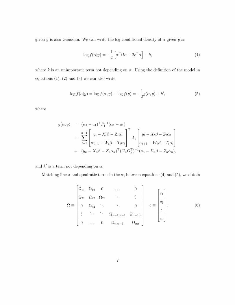
given y is also Gaussian. We can write the log conditional density of α given y as

log f(α|y) = −12

[α>Ωα− 2c>α

]+ k, (4)

where k is an unimportant term not depending on α. Using the definition of the model in

equations (1), (2) and (3) we can also write

log f(α|y) = log f(α, y)− log f(y) = −12g(α, y) + k′, (5)

where

g(α, y) = (α1 − a1)>P−11 (α1 − a1)

+n−1∑t=1

yt −Xtβ − Ztαt

αt+1 −Wtβ − Ttαt

>

At

yt −Xtβ − Ztαt

αt+1 −Wtβ − Ttαt

+ (yn −Xnβ − Znαn)>(GnG

>n )−1(yn −Xnβ − Znαn),

and k′ is a term not depending on α.

Matching linear and quadratic terms in the αt between equations (4) and (5), we obtain

Ω ≡

Ω11 Ω12 0 . . . 0

Ω21 Ω22 Ω23. . .

...

0 Ω32. . . . . . 0

.... . . . . . Ωn−1,n−1 Ωn−1,n

0 . . . 0 Ωn,n−1 Ωnn

c ≡

c1

c2...

cn

, (6)

7

where

Ωtt ≡ Z>t A11,tZt + Z>t A12,tTt + T>t A21,tZt + T>t A22,tTt +A22,t−1, t = 1, . . . , n− 1,

Ωnn ≡ Z>n A11,nZn +A22,n−1,

Ωt+1,t ≡ −A21,tZt −A22,tTt, t = 1, . . . , n− 1,

Ωt,t+1 ≡ −Z>t A12,t − T>t A22,t, t = 1, . . . , n− 1,

c1 ≡ (Z>1 A11,1 + T>1 A21,1)(y1 −X1β)− (Z>1 A12,1 + T>1 A22,1)(W1β)

+ A22,0(W0β + T0α0),

ct ≡ (Z>t A11,t + T>t A21,t)(yt −Xtβ)− (Z>t A12,t + T>t A22,t)(Wtβ)

−A21,t−1(yt−1 −Xt−1β) +A22,t−1(Wt−1β), t = 2, . . . , n− 1,

cn ≡ Z>n A11,n(yn −Xnβ)−A21,n−1(yn−1 −Xn−1β) +A22,n−1(Wn−1β).

3 Two Precision-Based Methods for Simulation Smoothing

Here we discuss two methods for state smoothing using the precision Ω and covector c

of the conditional distribution of α given y. The first method is due to Rue (2001), who

considers the more general problem of drawing Gaussian Markov random fields. The second

method, introduced here, offers new insights and more efficient draws for the special case

of Gaussian linear state-space models.

8

Rue (2001) introduces a simple procedure for drawing a Gaussian random vector α with

a band-diagonal precision matrix Ω. We let N be the length of α and b be the number

of non-zero subdiagonals. By symmetry, the bandwidth of Ω is 2b + 1. The first step is

to compute the Cholesky decomposition Ω = LL> using an algorithm that exploits the

band diagonal structure. The next step is to solve the equation ε = L>α∗ for α∗, where

ε ∼ N(0, IN ), using band back-substitution. Then α∗ + µ, where µ is the mean of α, is a

draw from the distribution of α. If the covector c of α is readily available but not µ, one

can solve for µ in the equation LL>µ = c using band back-substitution twice. Rue (2001)

recognizes that the vector of states α in Gaussian linear state-space models is an example

of a Gaussian Markov random fields. The previous section explicitly derives Ω and c. We

note that for the state-space model defined in the introduction, N = nm and b = 2m− 1.

We now introduce another method for drawing α based on the precision and covector

of its conditional distribution of α given y. We draw the αt backwards, each αt from the

distribution αt|αt+1, . . . , αn, y. The following result, proved in Appendix A, allows us to

draw α and evaluate E[α|y] in time n.

Result 3.1 If α|y ∼ N(Ω−1c,Ω−1), where Ω has the block band structure of equation (6),

then

αt|αt+1, . . . , αn, y ∼ N(mt − ΣtΩt,t+1αt+1,Σt) and E[α|y] = (µ>1 , . . . , µ>n )>,

where

Σ1 = (Ω11)−1, m1 = Σ1c1,

Σt = (Ωtt − Ωt,t−1Σt−1Ωt−1,t)−1, mt = Σt(ct − Ωt,t−1mt−1),

µn = mn, µt = mt − ΣtΩt,t+1µt+1.

9

The result is related to a Levinson-like algorithm introduced by Vandebril, Mastronardi,

and Van Barel (2007). Their algorithm solves the equation Bx = y, where B is an n × n

symmetric band diagonal matrix and y is a n× 1 vector. Result 3.1 extends the results in

Vandebril, Mastronardi, and Van Barel (2007) in two ways. First, we modify the algorithm

to work with m ×m submatrices of a block band diagonal matrix rather than individual

elements of a band diagonal matrix. Second, we use intermediate quantities computed

while solving the equation Ωµ = c for µ = E[α|y] in order to compute E[αt|αt+1, . . . , αn, y]

and Var[αt|αt+1, . . . , αn, y].

We can now use the following algorithm to draw α from α|y (MMP method hereafter).

1. Compute Σ1 = (Ω11)−1, m1 = Σ1c1.

2. For t = 2, . . . , n, compute Σt = (Ωtt−Ωt,t−1Σt−1Ωt−1,t)−1, mt = Σt(ct−Ωt,t−1mt−1).

3. Draw αn ∼ N(mn,Σn).

4. For t = n− 1, . . . , 1, draw αt ∼ N(mt − ΣtΩt,t+1αt+1,Σt).

4 Efficiency Analysis

We compare the computational efficiency of various methods for drawing α|y. We consider

separately the fixed computational cost that is incurred only once, no matter how many

draws are needed, and the marginal computational cost required for an additional draw.

We do this because there are some applications, such as Bayesian analysis of state-space

models using Gibbs sampling, in which only one draw is needed and other applications,

such as importance sampling in non-Gaussian models, where many draws are needed.

We compute the cost of various matrix operations in terms of the number of floating

point multiplications required per observation. All the methods listed in the introduction

10

have fixed costs that are third order polynomials in p and m. The methods of Rue (2001),

Durbin and Koopman (2002) and the present paper all have marginal costs that are second

order polynomials in p and m. We will ignore fixed cost terms of lower order than three

and marginal cost terms of lower order than two. The marginal costs are only important

when multiple draws are required.

We take the computational cost of multiplying an N1 × N2 matrix by an N2 × N3

matrix as N1N2N3 scalar floating-point multiplications. If the result is symmetric or if one

of the matrices is triangular, we divide by two. It is possible to multiply matrices more

efficiently, but the dimensions required before realizing savings are higher than those usually

encountered in state-space models. We take the cost of the Cholesky decomposition of a full

N×N matrix as N3/6 scalar multiplications, which is the cost using the algorithm in Press,

Teukolsky, Vetterling, and Flannery (1992, p. 97). When the matrix has bandwidth 2b+1,

the cost is Nb2/2. Solving a triangular system of N equations using back-substitution

requires N2/2 scalar multiplications. When the triangular system has bandwidth b + 1,

only Nb multiplications are required.

4.1 Fixed Costs

We first consider the cost of computing the precision Ω and covector c, which is required

for the methods of Rue (2001) and the current paper.

The cost depends on how we specify the variance of vt, the stacked innovation. The

matrices Gt and Ht are more convenient for methods using the Kalman filter, while the

precisions At are most useful for the precision-based methods. We recognize that it is often

easier to specify the innovation distribution in terms of Gt and Ht rather than At. In most

cases, however, the At are diagonal, constant, or take on one of a small number of values,

and so the additional computation required to obtain the At is negligible.

11

There is an important case where it is more natural to provide the At. Linear Gaus-

sian state-space models may be used to facilitate estimation in non-linear or non-Gaussian

state-space models by providing proposal distributions for MCMC methods or importance

distributions for importance sampling applications. In these cases, precisions in the ap-

proximating Gaussian model are negative Hessian matrices of the log observation density

of the non-Gaussian or non-linear model. See Durbin and Koopman (1997) and Section 5

of the present paper.

In general, calculation of the Ωtt and Ωt,t+1 is computationally demanding. However,

in many cases of interest, At, Zt and Tt are constant, or take on one of a small number of

values. In these cases, the computational burden is a constant, not depending on n. We do

need to compute each ct, but provided that the matrix expressions in parantheses in the

equations following (6) can be pre-computed, this involves matrix-vector multiplications,

whose costs are only second order polynomials in p and m.

We now consider the cost of the Kalman filter, which is used in most methods for

simulation smoothing. The computations are as follows:

et = yt − [Xtβ]− Ztat, Dt = ZtPtZ>t + [GtG

>t ],

Kt = (TtPtZ>t + [HtG

>t ])D−1

t , Lt = Tt −KtZt,

at+1 = [Wtβ] + Ttat +Ktet, Pt+1 = [TtPt]L>t + [HtH>t ] + [HtG

>t ]Kt

Here and elsewhere, we use braces to denote quantities that do not need to be computed

for each observation. These include quantities such as [TtPt] above that are computed in

previous steps, and quantities such as [HtH>t ] that are usually either constant or taking

values in a small pre-computable set.

Table 1 lists the matrix-matrix multiplications, Cholesky decompositions, and solutions

12

of triangular systems required for three high level operations: an iteration of the Kalman

filter, the computation of Ω = LL> using standard methods for band diagonal Ω, and

the computation of the Σt and mt of Result 3.1. All simulation smoothing methods we

are aware of use one of these high-level operations. We represent the solution of trian-

gular systems using notation for the inverse of a triangular matrix, but no actual matrix

inversions are performed, as this is inefficient. The table also gives the number of scalar

multiplications for each operation as a function of p and m. Terms of less than third order

are omitted, so we ignore matrix-vector multiplications, whose costs are mere second order

monomials in m and p.

There are special cases where the Kalman filter computations are less costly. In some

of these, the elements of Tt and Zt are zero or one, and certain matrix multiplications do

not require any scalar multiplications. In others, certain matrices are diagonal, reducing

the number of multiplications by an order.

The relative efficiency of precision-based methods compared with Kalman filter based

methods depends on various features of the application. We see that the precision-based

methods have no third order monomials involving p. For the MMP method, the coefficient

of the m3 term is 7/6, compared with 2 for the CFA and 2 for the Kalman filter if TtPt

is a general matrix multiplication. If Tt is diagonal or composed of zeros and ones, the

coefficient of m3 drops to 1 for the Kalman filter.

4.2 Marginal Costs

Compared with the fixed cost of pre-processing, the marginal computational cost of an

additional draw from α|y is negligible for all three methods we consider. In particular, no

matrix-matrix multiplications, matrix inversions, or Cholesky decompositions are required.

However, when large numbers of these additional draws are required, this marginal cost

13

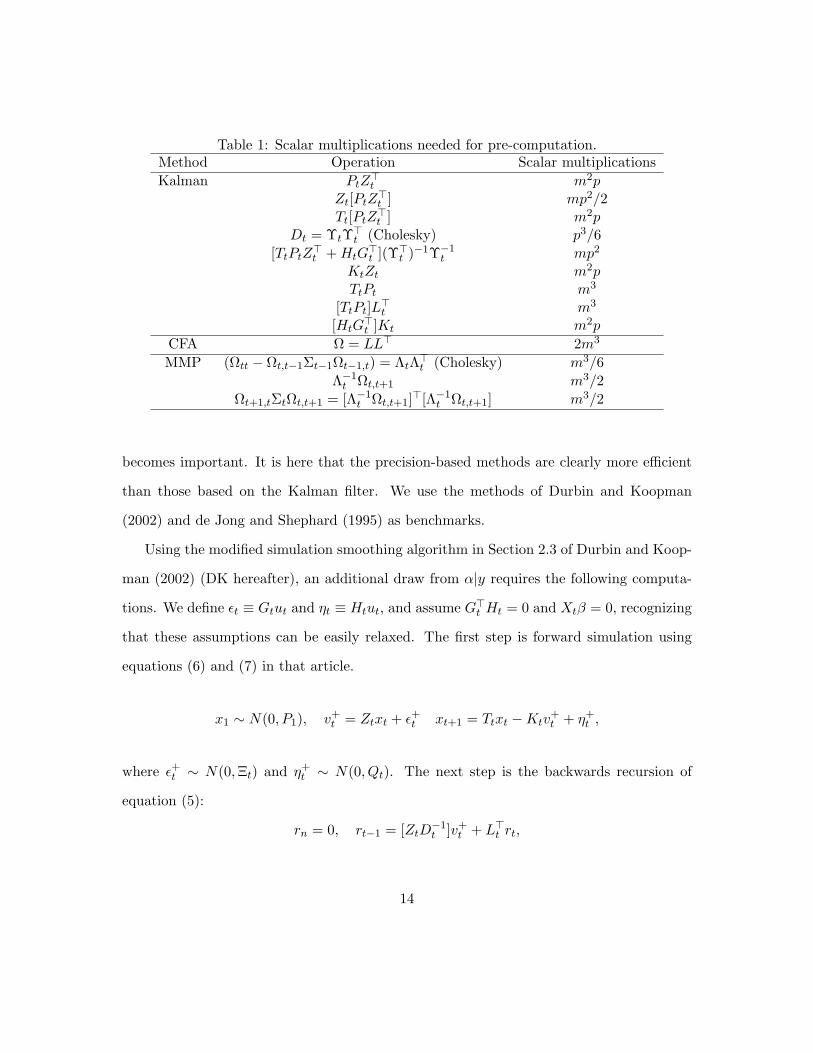
Table 1: Scalar multiplications needed for pre-computation.Method Operation Scalar multiplicationsKalman PtZ

>t m2p

Zt[PtZ>t ] mp2/2

Tt[PtZ>t ] m2p

Dt = ΥtΥ>t (Cholesky) p3/6[TtPtZ

>t +HtG

>t ](Υ>t )−1Υ−1

t mp2

KtZt m2pTtPt m3

[TtPt]L>t m3

[HtG>t ]Kt m2p

CFA Ω = LL> 2m3

MMP (Ωtt − Ωt,t−1Σt−1Ωt−1,t) = ΛtΛ>t (Cholesky) m3/6Λ−1

t Ωt,t+1 m3/2Ωt+1,tΣtΩt,t+1 = [Λ−1

t Ωt,t+1]>[Λ−1t Ωt,t+1] m3/2

becomes important. It is here that the precision-based methods are clearly more efficient

than those based on the Kalman filter. We use the methods of Durbin and Koopman

(2002) and de Jong and Shephard (1995) as benchmarks.

Using the modified simulation smoothing algorithm in Section 2.3 of Durbin and Koop-

man (2002) (DK hereafter), an additional draw from α|y requires the following computa-

tions. We define εt ≡ Gtut and ηt ≡ Htut, and assume G>t Ht = 0 and Xtβ = 0, recognizing

that these assumptions can be easily relaxed. The first step is forward simulation using

equations (6) and (7) in that article.

x1 ∼ N(0, P1), v+t = Ztxt + ε+t xt+1 = Ttxt −Ktv

+t + η+

t ,

where ε+t ∼ N(0,Ξt) and η+t ∼ N(0, Qt). The next step is the backwards recursion of

equation (5):

rn = 0, rt−1 = [ZtD−1t ]v+

t + L>t rt,

14

and the computation of residuals in equation (4):

η+t = Qtrt.

A draw η from the conditional distribution of η given y is given by

η = η − η+ + η+,

where η is a pre-computed vector. To construct a draw α from the conditional distribution

of α given y, we use

α1 = α1 − P1r0 + x1, αt+1 = Ttαt + ηt,

where α1 is pre-computed.

de Jong and Shephard (1995) (DeJS hereafter) draw α|y using the following steps, given

in equation (4) of their paper. First εt is drawn from N(0, σ2Ct), where the Cholesky factor

of σ2Ct can be pre-computed. Then rt is computed using the backwards recursion

rt−1 = [Z>t D−1t et] + L>t rt − [V >t C

−1t ]εt.

Next, αt+1 is computed as

αt+1 = [Wtβ] + Ttαt + Ωtrt + εt.

In our approach, we draw, for each observation, a vector vt ∼ N(0, Im) and compute

αt = mt − [ΣtΩt,t+1]αt+1 + Λ−1t vt.

15

Computing Λ−1t vt using Λt (which is triangular, see Table 1) requires m(m−1)/2 multipli-

cations and m floating point divisions. If we are making multiple draws, we can compute

the reciprocals of the diagonal elements of Λt once and convert the divisions into multipli-

cations, which are typically much less costly.

The band back-substitution used by Rue (2001) is quite similar to this. However, it is

a little less efficient if one is using standard band back-substitution algorithms. These do

not take advantage of the special structure of state-space models, for which Ω has elements

equal to zero in its first 2m− 1 subdiagonals.

5 An Empirical Application to Count Models

Durbin and Koopman (1997) show how to compute an arbitrarily accurate evaluation of

the likelihood function for a semi-Gaussian state-space model in which the state evolves

according to equation (2), but the conditional distribution of observations given states is

given by a general distribution with density (or mass) function p(y|α). To simplify, we

suppress notation for the dependence on θ, the vector of parameters.

The approach is as follows. The first step is to construct a fully Gaussian state-space

model with the same state dynamics as the semi-Gaussian model but with a Gaussian

measurement equation of the following form:

yt = µt + Ztαt + εt, (7)

where the εt are independent N(0,Ξt) and independent of the state equation innovations.

The Zt are matrices such that the distribution of y given α depends only on the Ztαt. They

choose µt and Ξt such that the implied conditional density g(y|α) approximates p(y|α) as

a function of α near the mode of p(α|y). The next step is to draw a sample of size N from

16

the conditional distribution of α given y for the fully Gaussian state-space model. The

final step is to use this sample as an importance sample to approximate the likelihood for

the semi-Gaussian model.

The Gaussian measurement density g(y|α) is chosen such that log g(y|α) is a quadratic

approximation of log p(y|α), as a function of α, at the mode α of the density p(α|y). Durbin

and Koopman (1997) find this density by iterating the following steps until convergence to

obtain µt and Ξt:

1. Using the current values of the µt and Ξt, compute α = Eg[α|y], where Eg denotes

expectation with respect to the Gaussian density g(α|y). Durbin and Koopman

(1997) use routine Kalman filtering and smoothing with the fully Gaussian state-

space model to find α.

2. Using the current α, compute the µt and Ξt such that log p(y|α) and log g(y|α) have

the same gradient and Hessian (with respect to α) at α. Durbin and Koopman (1997)

show that µt and Ξt solve the following two equations:

∂ log p(yt|αt)∂(Ztαt)

− Ξ−1t (yt − Ztαt − µt) = 0, (8)

∂2 log p(yt|αt)∂(Ztαt)∂(Ztαt)′

+ Ξ−1t = 0. (9)

It is interesting to note that this delivers the specification of the measurement equation

error of the fully Gaussian model directly in terms of the precision Ξ−1t rather than the

variance Ξt directly.

The likelihood function L(θ) we wish to evaluate is

L(θ) = p(y) =∫p(y, α)dα =

∫p(y|α)p(α)dα. (10)

17

Durbin and Koopman (1997) employ importance sampling to efficiently and accurately

approximate the above integrals. The likelihood for the approximating Gaussian model is

Lg(θ) = g(y) =g(y, α)g(α|y)

=g(y|α)p(α)g(α|y)

. (11)

Substituting for p(α) from (11) into (10) gives

L(θ) = Lg(θ)∫p(y|α)g(y|α)

g(α|y)dα = Lg(θ)Eg[w(α)], (12)

where

w(α) ≡ p(y|α)g(y|α)

.

One can generate a random sample α(1), . . . , α(N) from the density g(α|y) using any of the

methods for drawing states in fully Gaussian models. An unbiased Monte Carlo estimate

of L(θ) is

L1(θ) = Lg(θ)w, (13)

where w = N−1∑N

i=1w(α(i)).

It is usually more convenient to work with the log-likelihood, and we can write

log L1(θ) = logLg(θ) + log w. (14)

However, E[log w] 6= logEg[w(α(i)], so (14) is a biased estimator of logL(θ).

Durbin and Koopman (1997) propose an approximately unbiased estimator of logL(θ)

18

given by

log L2(θ) = logLg(θ) + log w +s2w

2Nw2, (15)

where s2w is an estimator of the variance of the w(α(i)) given by

s2w =1

N − 1

N∑i=1

(w(α(i))− w)2.

5.1 Modifications to the Algorithm for Approximating L(θ)

We propose here three modifications of the Durbin and Koopman (1997) method for ap-

proximating L(θ). The modified method does not involve Kalman filtering.

First, we use the MMP algorithm to draw α from its conditional distribution given y.

Second, we compute Lg(θ) as the extreme right hand side of equation (11). The equation

holds for any value of α; convenient choices which simplify computations include the prior

mean and the posterior mean.

Finally, in the rest of this section we present a method for computing the µt and Ξt of

the fully Gaussian state-space model. It is based on a multivariate normal approximation

of p(α|y) at its mode α and the application of Result 3.1. It is computationally more

efficient than Kalman filtering and smoothing.

We first compute α by iterating the following steps until convergence.

1. Using the current value of α, find the precision ¯H and co-vector ¯c of a Gaussian

approximation to p(α|y) based on a second-order Taylor expansion of log p(α) +

log p(y|α) around the point α.

2. Using the current values of ¯H and ¯c, compute µ = ¯H−1¯c, the mean of the Gaussian

approximation, using Result 3.1.

19

We then use equations (8) and (9) to compute the µt and Ξt.

We compute the precision ¯H as H + H, and the co-vector ¯c as c + c, where H and c

are the precision and co-vector of the marginal distribution of α (detailed formulations are

provided for our example in the next section), and H and c are the precision and co-vector

for a Gaussian density approximating p(y|α) as a function of α up to a multiplicative

constant. Since H is block-diagonal and H is block-band-diagonal, ¯H is also block-band-

diagonal.

We compute H and c as follows. Let a(αt) ≡ −2 log[p(yt|αt)]. We approximate a(αt)

by a(αt), consisting of the first three terms of the Taylor expansion of a(αt) around αt:

a(αt) ≈ a(αt) = a(αt) +∂a(αt)∂αt

(αt − αt) +12

(αt − αt)′∂2a(αt)∂αt∂α′t

(αt − αt).

If we complete the square, we obtain

a(αt) = (αt − h−1t ct)′ht(αt − h−1

t ct) + k,

where

ht =12∂2a(αt)∂αt∂α′t

,

ct = htαt −12∂a(αt)∂αt

,

and k is an unimportant term not depending on αt. Note that ht and ct are the precision and

co-vector of a multivariate normal distribution with density proportional to exp[−12 a(αt)].

Since log p(y|α) is additively separable in the elements of α, it means that it is reason-

ably well approximated, as a function of α, by∏n

t=1 exp[−12 a(αt)], which is proportional

20

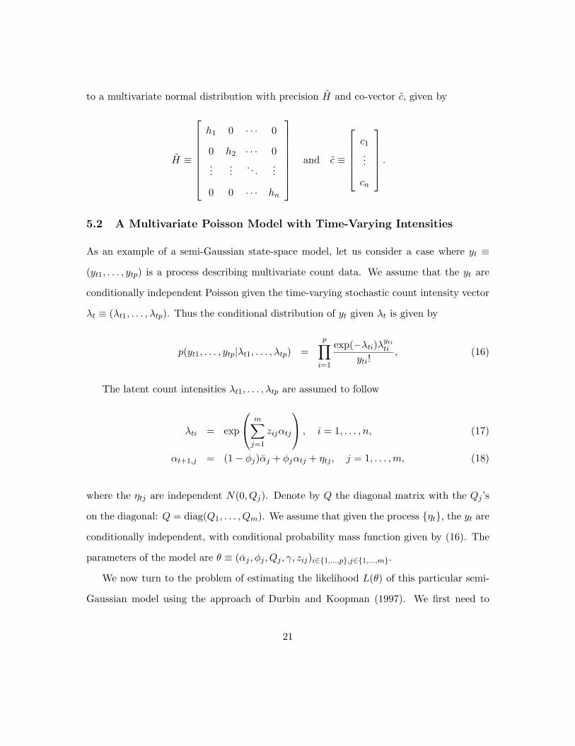
to a multivariate normal distribution with precision H and co-vector c, given by

H ≡

h1 0 · · · 0

0 h2 · · · 0...

.... . .

...

0 0 · · · hn

and c ≡

c1...

cn

.

5.2 A Multivariate Poisson Model with Time-Varying Intensities

As an example of a semi-Gaussian state-space model, let us consider a case where yt ≡

(yt1, . . . , ytp) is a process describing multivariate count data. We assume that the yt are

conditionally independent Poisson given the time-varying stochastic count intensity vector

λt ≡ (λt1, . . . , λtp). Thus the conditional distribution of yt given λt is given by

p(yt1, . . . , ytp|λt1, . . . , λtp) =p∏

i=1

exp(−λti)λytiti

yti!, (16)

The latent count intensities λt1, . . . , λtp are assumed to follow

λti = exp

m∑j=1

zijαtj

, i = 1, . . . , n, (17)

αt+1,j = (1− φj)αj + φjαtj + ηtj , j = 1, . . . ,m, (18)

where the ηtj are independent N(0, Qj). Denote by Q the diagonal matrix with the Qj ’s

on the diagonal: Q = diag(Q1, . . . , Qm). We assume that given the process ηt, the yt are

conditionally independent, with conditional probability mass function given by (16). The

parameters of the model are θ ≡ (αj , φj , Qj , γ, zij)i∈1,...,p,j∈1,...,m.

We now turn to the problem of estimating the likelihood L(θ) of this particular semi-

Gaussian model using the approach of Durbin and Koopman (1997). We first need to

21

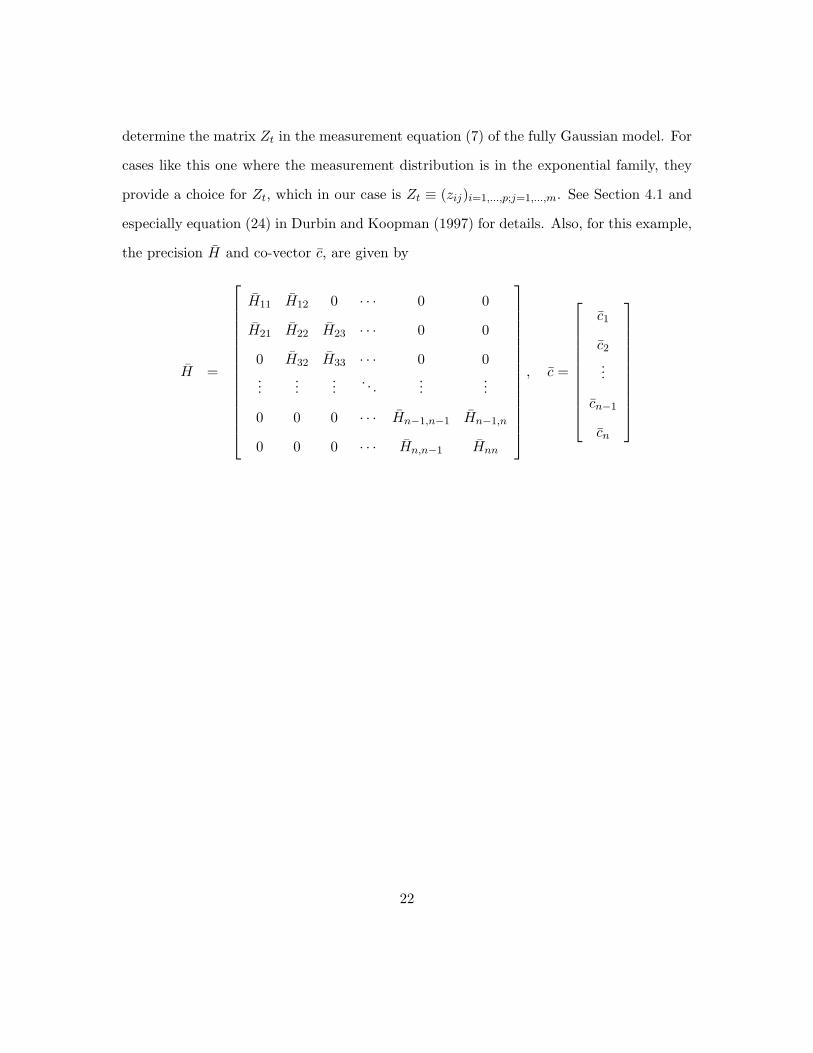
determine the matrix Zt in the measurement equation (7) of the fully Gaussian model. For

cases like this one where the measurement distribution is in the exponential family, they

provide a choice for Zt, which in our case is Zt ≡ (zij)i=1,...,p;j=1,...,m. See Section 4.1 and

especially equation (24) in Durbin and Koopman (1997) for details. Also, for this example,

the precision H and co-vector c, are given by

H =

H11 H12 0 · · · 0 0

H21 H22 H23 · · · 0 0

0 H32 H33 · · · 0 0...

......

. . ....

...

0 0 0 · · · Hn−1,n−1 Hn−1,n

0 0 0 · · · Hn,n−1 Hnn

, c =

c1

c2...

cn−1

cn

22

where

H11 = Hnn = Q−1,

Hjj =

(1 + φ2

1)/Q1 · · · 0...

. . ....

0 · · · (1 + φ2m)/Qm

, j = 2, . . . , n− 1,

Hj,j+1 = Hj+1,j =

−φ1/Q1 · · · 0

.... . .

...

0 · · · −φm/Qm

, j = 1, . . . , n− 1,

c1 = cn =

α1(1− φ1)/Q1

...

αm(1− φm)/Qm

,

cj =

α1(1− φ1)2/Q1

...

αm(1− φm)2/Qm

, j = 2, . . . , n− 1.

We compare the computational efficiency of all three methods for estimating the like-

lihood for this semi-Gaussian state-space model. We do so by counting computational

operations and profiling code.

Since a large number of draws from g(α|y) is required for a good approximation of L(θ),

we focus on the marginal computational cost of an additional draw. We will see that for

a typical number of draws, the computational overhead associated with the first draw is

small.

In the DeJS approach, one additional draw αt requires the following computations per

23

observation [see equation (5) of their paper]:

nt = [D−1t et]−K>t rt, εt = [C1/2

t ]N(0, Ip), ξt = Γtnt + εt,

Zαt = [yt − µt]− ξt, rt−1 = [Z ′D−1t et] + L′trt − [V ′tC

−1t ]εt.

In the DK approach, one additional draw requires the following computations per ob-

servation. (Here we do not simulate α but rather the Zαt, which we obtain more easily by

simulating the disturbances εt according to Section 2.3 of Durbin and Koopman (2002).)

There is a forward pass to simulate v+t :

v+t = µt + Zx+

t + ε+t , x+t+1 = Ttx

+t + η+

t −Ktv+t ,

where ε+t ∼ N(0,Ξt) and η+t ∼ N(0, Q). This is followed by a backward pass [see equations

(4) and (5) and Algorithm 1 of their paper]:

ε+t = Ξt(D−1t vt −K ′trt), rt−1 = [Z ′D−1

t ]v+t + L′trt,

εt = εt − ε+t + ε+t , Zαt = [yt − µt]− εt,

where εt is pre-computed.

In the MMP approach, one additional draw requires the following computations per

observation1:

αt = mt − [ΣtΩt,t+1]αt+1 + [Σ1/2t ]N(0, Im).

The computational costs per observation for an additional draw of αt are summarized in1Adding p×m multiplications for each of the Zαt, which are required to evaluate p(y|α).

24

Table 2: Computational costs per observation per additional draw of αt

Algorithm +/− × N0,1

DeJS 3p+ 2m (3p2 + p)/2 + 2mp+m2 pDK 6p+ 3m (5p2 + p)/2 + 4mp+ 2m+m2 p+mMMP 2m (3m2 +m)/2 + pm m

Table 2.

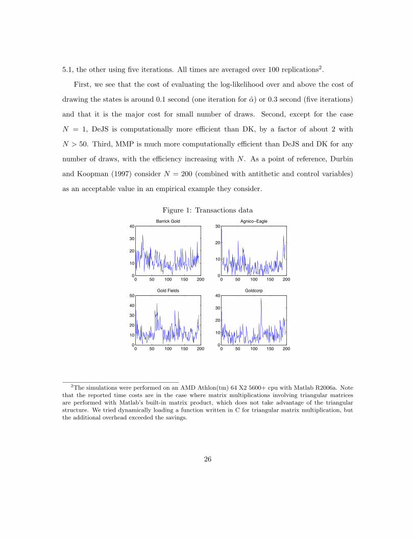
We profile code for all three methods to see how they perform in practice. We use

data on the number of transactions over consecutive two minute intervals for four different

stocks in the same industry. For one business day (November 6, 2003), we look at all the

transactions for four different gold-mining companies: Agnico-Eagle Mines Limited, Barrick

Gold Corporation, Gold Fields Limited and Goldcorp Inc. We use all the transactions

recorded during normal trading hours on the New York Stock Exchange Trade and Quote

database. This gives 195 observations for each series. The data are plotted in Figure 1.

We take the number of factors to be equal to the number of observed series. That is,

m = p = 4. To ensure identification, we impose zii = 1 and zij = 0 for j > i.

For all three methods, we compute α using the fast method presented in Section 5.1.

This puts all methods for drawing states on an equal footing. We point out, though, that

this gives a small advantage to the estimation of L(θ) using either the DeJS or DK methods,

relative to the case where the Kalman filter and simulation smoother are used to compute

α.

For various values of the size N of the importance sample, Table 3 gives the ratio of

the time cost in 100ths of seconds of (i) generating N draws of α(i) and (ii) the total cost

of evaluating the log-likelihood once, which consists of the former plus some overhead,

including the computation of µt, Ξt, α and the w(α(i)). For the latter, we report costs for

two different approximations of α: one using a single iteration of steps 1 and 2 in Section

25

5.1, the other using five iterations. All times are averaged over 100 replications2.

First, we see that the cost of evaluating the log-likelihood over and above the cost of

drawing the states is around 0.1 second (one iteration for α) or 0.3 second (five iterations)

and that it is the major cost for small number of draws. Second, except for the case

N = 1, DeJS is computationally more efficient than DK, by a factor of about 2 with

N > 50. Third, MMP is much more computationally efficient than DeJS and DK for any

number of draws, with the efficiency increasing with N . As a point of reference, Durbin

and Koopman (1997) consider N = 200 (combined with antithetic and control variables)

as an acceptable value in an empirical example they consider.

Figure 1: Transactions data

0 50 100 150 2000

10

20

30

40Barrick Gold

0 50 100 150 2000

10

20

30Agnico−Eagle

0 50 100 150 2000

10

20

30

40

50Gold Fields

0 50 100 150 2000

10

20

30

40Goldcorp

2The simulations were performed on an AMD Athlon(tm) 64 X2 5600+ cpu with Matlab R2006a. Notethat the reported time costs are in the case where matrix multiplications involving triangular matricesare performed with Matlab’s built-in matrix product, which does not take advantage of the triangularstructure. We tried dynamically loading a function written in C for triangular matrix multiplication, butthe additional overhead exceeded the savings.

26

Table 3: Time cost of drawing α(i) and the total cost of evaluating the likelihood, as afunction of the number of draws N . For the total time cost, numbers are reported whenperforming one and five iterations to obtain α. Figures are in 100ths of seconds.

Method N = 1 N = 10 N = 50 N = 150DeJS α draw 9.7 22.0 78.3 215.1

total (19.2–38.7) (31.9–51.7) (89.6–108.9) (229.2–253.6)DK α draw 7.1 34.6 156.6 462.9

total (16.7–36.6) (45.1–64.9) (168.1–185.7) (477.8–491.0)MMP α draw 4.6 10.0 34.9 103.5

total (14.6–33.9) (20.3–40.4) (46.5–65.5) (118.2–136.3)

6 Conclusion

In this paper we introduce a new method for drawing state variables in Gaussian state-

space models from their conditional distribution given parameters and observations. The

method is quite different from standard methods, such as those of de Jong and Shephard

(1995) and Durbin and Koopman (2002), that use Kalman filtering. It is much more in

the spirit of Rue (2001), who describes an efficient method for drawing Gaussian random

vectors with band diagonal precision matrices. As Rue (2001) recognizes, the distribution

α|y in linear Gaussian state-space models is an example.

Our first contribution is computing Ω and c for a widely used and fairly flexible state-

space model. These are required inputs for both the CFA of Rue (2001) and the method

we described here.

Our second contribution is a new precision-based state smoothing algorithm. It is

more computationally efficient for the special case of state-space models, and delivers the

conditional means E[αt|αt+1, . . . , αn, y] and conditional variances Var[αt|αt+1, . . . , αn, y]

as a byproduct. These conditional moments turn out to be very useful in an extension of

the method, described in McCausland (2008), to non-linear and non-Gaussian state-space

models with univariate states.

27

The algorithm is an extention of a Levinson-like algorithm introduced by Vandebril,

Mastronardi, and Van Barel (2007), for solving the equation Bx = y, where B is an

n × n symmetric band diagonal matrix and y is a n × 1 vector. The algorithm extends

theirs in two ways. First, we modify the algorithm to work with m × m submatrices of

a block band diagonal matrix rather than individual elements of a band diagonal matrix.

Second, we use intermediate quantities computed while solving the equation Ωµ = c for the

mean µ given the precision Ω and co-vector c in order to compute the conditional means

E[αt|αt+1, . . . , αn, y] and conditional variances Var[αt|αt+1, . . . , αn, y].

Our third contribution is a computational analysis of several state smoothing methods.

One can often precompute the Ωtt and Ωt,t+1, in which case the precision-based methods are

more efficient than those based on the Kalman filter. The advantage is particularly strong

when p is large or when several draws of α are required for each value of the parameters.

Kalman filtering, which involves solving systems of p equations in p unknowns, requires

O(p3) scalar multiplications. If the At can be pre-computed, or take on only a constant

number of values, the precision-based methods require no operations of higher order than

p2, in p. If the Zt and Tt can also be pre-computed, or take on only a constant number

of values, the order drops to p. For large m, our method involves half as many scalar

multiplications as CFA.

We consider an applications of our methods to the evaluation of the log-likelihood

function for a multivariate Poisson model with latent count intensities.

A Proof of Result 3.1

Suppose α|y ∼ N(Ω−1c,Ω−1) and define

Σ1 = (Ω11)−1, m1 = Σ1c1,

28

Σt = (Ωtt − Ωt,t−1Σt−1Ωt−1,t)−1, mt = Σt(ct − Ωt,t−1mt−1).

Now let µn ≡ mn and for t = n−1, . . . , 1, let µt = mt−ΣtΩt,t+1µt+1. Let µ = (µ>1 , . . . , µ>n )>.

We first show that Ωµ = c, which means that µ = E[α|y]:

Ω11µ1 + Ω12µ2 = Ω11(m1 − Σ1Ω12µ2) + Ω12µ2

= Ω11((Ω11)−1c1 − (Ω11)−1Ω12µ2) + Ω12µ2 = c1.

For t = 2, . . . , n− 1,

Ωt,t−1µt−1 + Ωttµt + Ωt,t+1µt+1

= Ωt,t−1(mt−1 − Σt−1Ωt−1,tµt) + Ωttµt + Ωt,t+1µt+1

= Ωt,t−1mt−1 + (Ωtt − Ωt,t−1Σt−1Ωt−1,t)µt + Ωt,t+1µt+1

= Ωt,t−1mt−1 + Σ−1t µt + Ωt,t+1µt+1

= Ωt,t−1mt−1 + Σ−1t (mt − ΣtΩt,t+1µt+1) + Ωt,t+1µt+1

= Ωt,t−1mt−1 + (ct − Ωt,t−1mt−1) = ct.

Ωn,n−1µn−1 + Ωnnµn = Ωn,n−1(mn−1 − Σn−1Ωn−1,nµn) + Ωnnµn

= Ωn,n−1mn−1 + Σ−1n µn

= Ωn,n−1mn−1 + Σ−1n mn

= Ωn,n−1mn−1 + (cn − Ωn,n−1)mn−1 = cn.

We will now prove that E[αt|αt+1, . . . , αn, y] = mt−ΣtΩt,t+1αt+1 and that Var[αt|αt+1, . . . , αn, y] =

29

Σt. We begin with the standard result

α1:t|αt+1:n, y ∼ N(µ1:t − Ω−1

1:t,1:tΩ1:t,t+1:n(αt+1:n − µt+1:n),Ω−11:t,1:t

),

where µ, α and Ω are partitioned as

µ =

µ1:t

µt+1:n

, α =

α1:t

αt+1:n

, Ω =

Ω1:t,1:t Ω1:t,t+1:n

Ωt+1:n,1:t Ωt+1:n,t+1:n

,with µ1:t, α1:t and Ω(11) having dimensions tm× 1, tm× 1, and tm× tm respectively. Note

that the only non-zero elements of Ω(12) come from Ωt,t+1. We can therefore write the

univariate conditional distribution αt|αt+1:n as

αt|αt+1:n ∼ N(µt − (Ω−11:t,1:t)ttΩt,t+1(αt+1 − µt+1), (Ω−1

1:t,1:t)tt).

The following inductive proof establishes the result Var[αt|αt+1, . . . , αn, y] = Σt:

(Ω11)−1 = Σ1

(Ω−11:t,1:t)tt = (Ωtt − Ωt,1:t−1Ω−1

1:t−1,1:t−1Ω1:t−1,t)−1

= (Ωtt − Ωt,t−1Σt−1Ωt−1,t)−1 = Σt.

As for the conditional mean,

E[αt|αt+1, . . . , αn, y] =

µt − ΣtΩt,t+1(αt+1 − µt+1) t = 1, . . . , n− 1

µn t = n.

30

By the definition of µt, mt = µt + ΣtΩt,t+1µt+1, so we obtain

E[αt|αt+1, . . . , αn, y] =

mt − ΣtΩt,t+1αt+1 t = 1, . . . , n− 1

mn t = n.

References

Boivin, J., and Giannoni, M. (2006). ‘DSGE Models in a Data-Rich Environment’, Working

Paper 12772, National Bureau of Economic Research.

Carter, C. K., and Kohn, R. (1994). ‘On Gibbs Sampling for State Space Models’,

Biometrika, 81(3): 541–553.

(1996). ‘Markov chain Monte Carlo in conditionally Gaussian State Space Models’,

Biometrika, 83(3): 589–601.

de Jong, P., and Shephard, N. (1995). ‘The Simulation Smoother for Time Series Models’,

Biometrika, 82(1): 339–350.

Durbin, J., and Koopman, S. J. (1997). ‘Monte Carlo maximum likelihood estimation for

non-Gaussian state space models’, Biometrika, 84(3): 669–684.

(2002). ‘A Simple and Efficient Simulation Smoother for State Space Time Series

Analysis’, Biometrika, 89(3): 603–615.

Forni, M., Hallin, M., Lippi, M., and Reichlin, L. (2000). ‘The Generalized Dynamic Factor

Model: Identification and Estimation’, Review of Economics and Statistics, 82(4): 540–

554.

Fruhwirth-Schnatter, S. (1994). ‘Data augmentation and Dynamic Linear Models’, Journal

of Time Series Analysis, 15: 183–202.

31

Fruhwirth-Schnatter, S., and Wagner, H. (2006). ‘Auxiliary mixture sampling for

parameter-driven models of time series of counts with applications to state space mod-

elling’, Biometrika, 93: 827–841.

Kim, S., Shephard, N., and Chib, S. (1998). ‘Stochastic Volatility: Likelihood Inference

and Comparison with ARCH Models’, Review of Economic Studies, 65(3): 361–393.

Knorr-Held, L., and Rue, H. (2002). ‘On Block Updating in Markov Random Field Models

for Disease Mapping’, Scandinavian Journal of Statistics, 29: 597–614.

McCausland, W. J. (2008). ‘The HESSIAN Method (Highly Efficient State Smoothing, In

A Nutshell)’, Cahiers de recherche du Departement de sciences economiques, Universite

de Montreal, no. 2008-03.

Press, W. H., Teukolsky, S. A., Vetterling, W. T., and Flannery, B. P. (1992). Numerical

recipes in C. Cambridge University Press, Cambridge, second edn., The art of scientific

computing.

Rue, H. (2001). ‘Fast Sampling of Gaussian Markov Random Fields with Applications’,

Journal of the Royal Statistical Society Series B, 63: 325–338.

Shephard, N., and Pitt, M. K. (1997). ‘Likelihood Analysis of Non-Gaussian Measurement

Time Series’, Biometrika, 84(3): 653–667.

Stock, J. H., and Watson, M. W. (1999). ‘Forecasting Inflation’, Journal of Monetary

Economics, 44: 293–335.

(2002). ‘Macroeconomic Forecasting Using Diffusion Indexes’, Journal of Business

and Economic Statistics, 20: 147–162.

32

Stroud, J. R., Muller, P., and Polson, N. G. (2003). ‘Nonlinear State-Space Models With

State-Dependent Variances’, Journal of the American Statistical Association, 98: 377–

386.

Vandebril, R., Mastronardi, N., and Van Barel, M. (2007). ‘A Levinson-like algorithm for

symmetric strongly nonsingular higher order semiseparable plus band matrices’, Journal

of Computational and Applied Mathematics, 198(1): 74–97.

33