simulation study of areal sweep efficiency...

SIMULATION STUDY OF AREAL SWEEP EFFICIENCY VERSUS A

FUNCTION OF MOBILITY RATIO AND ASPECT RATIO FOR STAGGERED

LINE-DRIVE WATERFLOOD PATTERN

A Thesis

by

RUSLAN GULIYEV

Submitted to the Office of Graduate Studies ofTexas A&M University

in partial fulfillment of the requirements for the degree of

MASTER OF SCIENCE

August 2008

Major Subject: Petroleum Engineering

SIMULATION STUDY OF AREAL SWEEP EFFICIENCY VERSUS A

FUNCTION OF MOBILITY RATIO AND ASPECT RATIO FOR STAGGERED

LINE-DRIVE WATERFLOOD PATTERN

A Thesis

by

RUSLAN GULIYEV

Submitted to the Office of Graduate Studies ofTexas A&M University

in partial fulfillment of the requirements for the degree of

MASTER OF SCIENCE

Approved by:

Chair of Committee, Daulat D. MamoraCommittee Members, Jerome J. Schubert

Luc T. IkelleHead of Department, Stephen A. Holditch

August 2008

Major Subject: Petroleum Engineering

iii

ABSTRACT

Simulation Study of Areal Sweep Efficiency Versus a Function

of Mobility Ratio and Aspect Ratio for Staggered

Line-drive Waterflood Pattern. (August 2008)

Ruslan Guliyev, B.S., Azerbaijan State Oil Academy

Chair of Advisory Committee: Dr. Daulat D. Mamora

Pattern geometry plays a major role in determining oil recovery during waterflooding

and enhanced oil recovery operations. Although simulation is an important tool for

design and evaluation, the first step often involves rough calculations based upon areal

sweep efficiencies of displacements in homogeneous, two-dimensional, scaled, physical

models. These results are available as a function of the displacement pattern and the

mobility ratio M.

In this research I studied the effect of mobility ratios on five-spot and staggered

waterflood patterns behavior for areal (2D) displacement in a reservoir that is

homogeneous and isotropic containing no initial gas saturation. Simulation was

performed using Eclipse 100 simulator.

Simulation results are presented as graphs of areal sweep efficiency at breakthrough

versus Craig mobility ratio for various staggered line drive aspect ratios.

The main results of the study are presented in the form of a graph of areal sweep

efficiency at breakthrough as a function of staggered line drive aspect ratio. This should

enable engineers to utilize the results in a convenient manner.

iv

ACKNOWLEDGEMENTS

I wish to express my sincere gratitude and appreciation to Dr. Daulat D. Mamora,

chair of my advisory committee, for his patience and continued support throughout my

research. I would also like to thank Dr. Jerome Schubert, member of my advisory

committee, for his encouragement to my research, his motivation and his “always-good

mood”. I also acknowledge Dr. Luc Ikelle, member of my advisory committee, for his

participation and guidance during my investigation. Finally, I want to express my

gratitude and appreciation to all my colleagues in Texas A&M University: Samir

Husseynzade, Faig Hasanov, and Mazen Barnawi.

v

TABLE OF CONTENTS

Page

ABSTRACT ...................................................................................................................... iii

ACKNOWLEDGEMENTS................................................................................................iv

TABLE OF CONTENTS ....................................................................................................v

LIST OF FIGURES ............................................................................................................vi

CHAPTER

I INTRODUCTION .......................................................................................1

1.1 Well patterns and mobility ratio ............................................................11.2 Areal sweep efficiency...........................................................................21.3 Displacement in a five-spot pattern .......................................................31.4 Displacement in a staggered pattern ......................................................5

II LITERATURE REVIEW.............................................................................6

2.1 Pitts, Gerald N., Crawford, Paul B. 1971, Simulation large flow networks in undergrownd media............................................................6 2.2 Bringham, William E., Kovscek, Anthony R., Wang, Yuandog 1998, A study of the effect of mobility ratios on pattern displacement behavior and streamline to infer permeability fields permeability media......................................................................................................7

III RESEARCH OBJECTIVES........................................................................8

IV SIMULATION AND CALCULATIONS...................................................9

4.1 Conditions and limitations .....................................................................94.2 Gridding .................................................................................................94.3 Methodology........................................................................................14 4.3.1 Oil-water relative permeability calculation ................................14 4.3.2 Fractional flow calculation .........................................................15 4.3.3 Mobility ratio calculation............................................................20 4.3.4 Breakthrough determination .......................................................20

vi

CHAPTER Page

V SIMULATION RESULTS ........................................................................29

VI SUMMARY, CONCLUSIONS AND RECOMMENDATIONS .............37

6.1 Summary..............................................................................................376.2 Conclusions..........................................................................................376.3 Recommendation .................................................................................38

NOMENCLATURE ..........................................................................................................39

REFERENCES ..................................................................................................................40

APPENDIX........................................................................................................................41

VITA..................................................................................................................................47

vii

LIST OF FIGURES

FIGURE Page

1.1 Illustration of waterflood patterns...............................................................................1

1.2 Single five-spot pattern(a), one-eight of a five-spot pattern (shaded) (b) .................4

1.3 Correlation of Areal Sweep Efficiency as a function of Craig water-oil mobility ratio for 5-spot patterns ................................................................................4

1.4 Single staggered line-drive pattern (a), and simplified one-eighth of a staggered line drive pattern (shaded) (b) ...................................................................5

4.1 Flood performance in one-eight of five-spot pattern with 20x10x1 model..............10



4.4 Flood performance in one-eight of staggered line-drive pattern with 60x30x1 model, d/a=0.75 .........................................................................................11

4.5 Flood performance in one-eight of staggered line-drive pattern with 60x30x1 model, d/a=1 ..............................................................................................12


4.7 Flood performance in one-eight of staggered line-drive pattern with 60x30x1 model, d/a=1.5 ...........................................................................................13


4.9 Corey-type relative permeability curves...................................................................14

4.10 Fractional flow curves for µo/µw ratio equal 0.2 and 0.5 ........................................16

4.11 Fractional flow curves for µo/µw ratio equal 1 and 2 ..............................................17

4.12 Fractional flow curves for µo/µw ratio equal 3 and 5 ..............................................18

4.13 Fractional flow curve for µo/µw ratio equal 10........................................................19

viii

FIGURE Page

4.14 Fractional flow fw versus WiD for viscosity ratios µo/µw equal 0.2 and 0.5 .............21

4.15 Fractional flow fw versus WiD for viscosity ratios µo/µw equal 1 and 2 ...................22

4.16 Fractional flow fw versus WiD for viscosity ratios µo/µw equal 3 and 5 ...................23

4.17 Fractional flow fw versus WiD for viscosity ratio µo/µw equal 10 ............................24

4.18 Wi versus fractional flow fw for viscosity ratios µo/µw equal 0.2 and 0.5 ................25

4.19 Wi versus fractional flow fw for viscosity ratios µo/µw equal 1 and 2 ......................26

4.20 Wi versus fractional flow fw for viscosity ratios µo/µw equal 3 and 5 ......................27

4.21 Wi versus fractional flow fw for viscosity ratio µo/µw equal 10 ...............................28

5.1 Comparison of Eclipse simulation results for 40x20x1 model with experimental values in five-spot waterflood pattern.................................................30

5.2 Comparison of Eclipse simulation results for 60x30x1 model with experimental values in five-spot waterflood pattern ................................................31

5.3 Illustration and comparison of five-spot pattern behavior for different grid models with Craig model..........................................................................................32

5.4 Comparison of 40x20x1 staggered line drive patterns simulation results for different aspect ratios (d/a) with Dyes experimental values for d/a=1.....................33

5.5 Comparison of 60x30x1 staggered line drive patterns simulation results for different aspect ratios (d/a) with Dyes experimental values for d/a=1.....................34

5.6 Comparison of 40x20x1 model’s flood efficiency for unit mobility ratio (M=1) ...36

5.7 Comparison of 60x30x1 model’s flood efficiency for unit mobility ratio (M=1) ...36

1

CHAPTER I

INTRODUCTION

1.1 Well patterns and mobility ratio

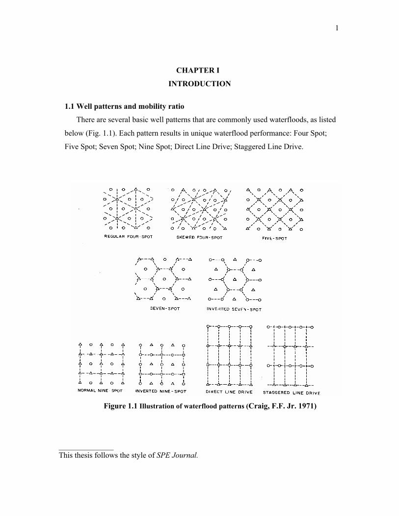
There are several basic well patterns that are commonly used waterfloods, as listed

below (Fig. 1.1). Each pattern results in unique waterflood performance: Four Spot;

Five Spot; Seven Spot; Nine Spot; Direct Line Drive; Staggered Line Drive.

Figure 1.1 Illustration of waterflood patterns (Craig, F.F. Jr. 1971)

______________This thesis follows the style of SPE Journal.

2

In a waterflood, water is injected in a well or pattern of wells to displace oil towards

a producer. When the leading edge of the waterflood front reaches the producer

breakthrough occurs (the first appearance of water in the produced fluids). After

breakthrough, both oil and water are produced and the watercut increases progressively.

The main objective of enhanced oil recovery (EOR) is to economically increase

displacement and areal sweep efficiency. A key factor is the mobility ratio - M.

The mobility ratio is simply the ratio of the mobility of the displacing phase to that

of the displaced or resident phase.

M ep =roe

o

w

rwe

k

k

. . . . . . . . . . . . . . . . . . . . . . . . . . . . (1.1)

Where Mep is end point mobility ratio; krwe and kroe are end point relative

permeability for water and oil respectively; µo and µw are water and oil insitu

viscosities. Mobility ratio is a function of viscosity and relative permeability, which in

turn depends on saturation. A variation of mobility ratio is Craig’s mobility ratio - Mc,

defined as:

Mc =ro

o

w

wrw

k

Sk

)( . . . . . . . . . . . . . . . . . . . . . . . . . . . . (1.2)

Where krw(Sw) is the water relative permeability at the average saturation behind the

flood front.

1.2 Areal sweep efficiency

For piston-like displacement, the areal sweep efficiency is:

EA AS / AT . . . . . . . . . . . . . . . . . . . . . . . . . . . . . . . . (1.3)

Where AS is the swept area and AT is the total area. Before and at breakthrough, the

amount of displacing fluid injected is equal to the displaced fluid produced,

disregarding compressibility. Assuming piston-like displacement, injected volume is

related to area swept.

3

Wi AS h Swc – Sor) . . . . . . . . . . . . . . . . . . . . . . . . . . . (1.4)

Where Wi is the volume of displacing fluid injected, h is the thickness of the

formation, and is porosity. Hence,

EA AS / AT Wi / (AT h Swc – Sor)) . . . .. . . . . . . . . . (1.5)

After breakthrough,

EA (Wi WP ) / ( AT h Swc – Sor)) . . . . . . . . . . . . . . . (1.6)

Where WP is volume of displacing fluid produced.

1.3 Displacement in a five-spot pattern

Analysis of a five-spot pattern in a reservoir can be simplified by examining the

behavior of a single five-spot pattern. A regular five-spot pattern consists of a

production well surrounded by four injection wells. It is assumed that the injection rates

are equal to the production rates. Thus flow is symmetric around each injection well

with 0.25 of the injection rate from each well confined to the pattern (Fig. 1.2).

Further simplifications are possible. A line drawn from injection well to production

well subdivides a quadrant into two symmetrical parts. Thus displacement performance

of one-eighth of a five-spot pattern is used to estimate the behavior of the full pattern.

In simulation, use of one-eight model will result in significant saving in CPU time.

4

a. b. Figure 1.2 Single five-spot pattern (a), one-eight of a five-spot pattern (shaded) (b)

Areal sweep efficiency and oil recovery efficiency at breakthrough are readily

determined from the correlations that have been developed from experiments with

scaled laboratory models.

Figure 1.3 Correlation of areal sweep efficiency as a function of Craig water oil mobility ratio for five-spot patterns (Forrest F. Craig. Jr. 1971)

a

a

5

A convenient way of estimating EAbt is to use the expression for the correlation

graphed in Fig. 1.3, which is as follows.

EAbt = 0.54602036 + cMc

MeM c

00509693.030222997.003170817.0

. . . (1.7)

1.4 Displacement in a staggered pattern

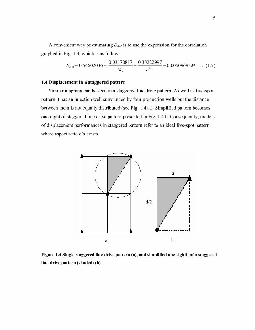
Similar mapping can be seen in a staggered line drive pattern. As well as five-spot

pattern it has an injection well surrounded by four production wells but the distance

between them is not equally distributed (see Fig. 1.4 a.). Simplified pattern becomes

one-eight of staggered line drive pattern presented in Fig. 1.4 b. Consequently, models

of displacement performances in staggered pattern refer to an ideal five-spot pattern

where aspect ratio d/a exists.

a. b.

Figure 1.4 Single staggered line-drive pattern (a), and simplified one-eighth of a staggered

line-drive pattern (shaded) (b)

a

d/2

6

CHAPTER II

LITERATURE REVIEW

Not many studies were directed to develop relations between areal sweep efficiency

and reservoir or fluid characterization parameters especially for different staggered

pattern distribution. Most notable works on staggered line drive are described below.

2.1 Pitts, Gerald N., Crawford, Paul B. 1971, Simulating large flow networks in

underground media

This study describes the possible effect of heterogeneous media on the areal sweep

efficiencies for different pattern distributions. The direct streamline method was applied

to three well known reservoir patterns: five-spot, direct-line drive (square) and

staggered line drive patterns. Each pattern was simulated with three different

permeability ranges. The ranges were (a) 100 to 50 md, (b) 100 to 1.0 md and (c) 100 to

0. 1 md. These distributions were used along with a random process to distribute the

permeabilities throughout a 20 x 20 matrix yielding a 400 block system.

It was found that areal sweeps for very heterogeneous five-spot patterns were

reduced to nearly 25 percent or about one-third of the sweep expected in homogeneous

media.

The heterogeneous staggered line drive pattern gave surprisingly low areal sweeps,

the average areal sweep for the (100 to 50) md range was 76 percent, 65 percent for the

(100 to 1.0) md range, and 26 percent sweep for the (100 to 0.1) md range. The two

smaller permeability ranges resulted in a larger areal sweep for the staggered line-drive

than the five-spot or direct-line drive patterns. However, for the wide permeability

range of (100 to 0. 1), about the same areal sweep was obtained for the staggered-line

drive and the five-spot patterns, but both gave smaller sweeps than the direct-line drive

square pattern.

7

2.2 Brigham, William E., Kovscek, Anthony R., Wang, Yuandong 1998, A study of

the effect of mobility ratios on pattern displacement behavior and streamline to

infer permeability fields permeability media

In this particular research it was found that for unit mobility ratio, unfavorable

mobility ratios and some favorable mobility ratios (M 0.3) in a staggered line-drive

pattern has higher areal sweep efficiency than a five-spot pattern. However, for very

favorable mobility ratios (M 0.3), a five-spot pattern has better sweep efficiency than

a common staggered-line-drive. The reason for this behavior was the change of

streamline and pressure distributions with mobility ratios. For very favorable mobility

ratios, the displacing front is near an isobar and intersects the pattern boundary at 90

degrees. That causes the fronts at times near breakthrough to become radial around the

producer for a five-spot pattern. This displacing front shape is due to the symmetry of

the five-spot pattern. Also, noticed more numerical dispersion in results for unfavorable

mobility ratio cases (M > 1).

For a staggered line drive, the displacing front is also perpendicular to the border of

the pattern. However, because the pattern is not symmetric, sweepout at breakthrough is

not complete. So theoretically it seems that only in the limit of very large d/a will the

areal sweep efficiency approach 1.

8

CHAPTER III

RESEARCH OBJECTIVES

The main objective of this research is to determine the areal sweep efficiency versus

mobility ratio distribution for different aspect ratios by simulating simplified (one-

eight) staggered line drive patterns using Schlumberger Eclipse 100 commercial

simulator. The results obtained should be useful for estimating areal sweep efficiency at

breakthrough when one is designing a staggered line-drive waterflood. To determine

the affect of grid number on simulation results all simulation runs will be performed for

three cases where grid distributions are 20x10x1, 40x20x1 and 60x30x1 where areas for

all cases are equal.

9

CHAPTER IV

SIMULATION AND CALCULATIONS

To simulate the displacement for the five-spot and staggered line-drive patterns we

will use Eclipse 100 with a two-dimensional grid distribution.

4.1 Conditions and limitations

The main features of the simulation model and runs are as follows:

1. Two dimensional where area equal 40 acres and thickness is 20 feet.

2. Incompressible displacement.

3. Homogeneous permeability field, i.e., k is constant and equal 30%.

4. No gas presents initially, Sgi=0.

5. Constant injection and production rates, Qi=Qp.

6. Relative permeability curves described with Corey-type equations.

7. Oil to water viscosity ratio µo/µw (where µw =1cp) is reciprocal of oil viscosity that

will have values: 0.2; 0.5; 1; 2; 3; 5 and 10 cp.

8. 1/8th of the basic unit described by a triangular Cartesian grid block.

9. Three cases were studied: 20x10x1, 40x20x1 and 60x30x1.

4.2 Gridding

In this research I built five staggered grid patterns for each grid distribution where

aspect ratio (d/a) will change linearly: 0.75; 1; 1.25; 1.5 and 1.75.

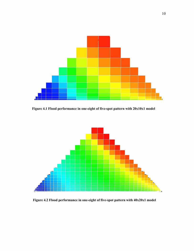
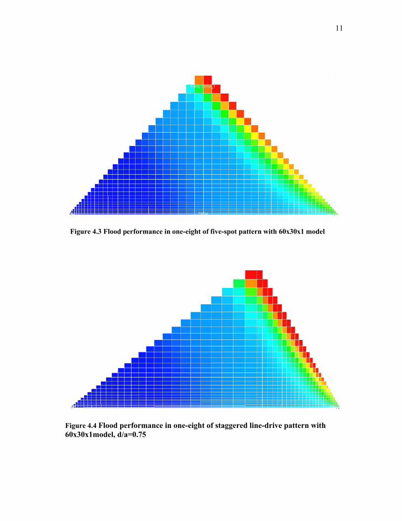
Fig. 4.1, Fig. 4.2 and Fig. 4.3 illustrate waterflood performance in simplified five-

spot patterns for different grid distribution: 20x10x1, 40x20x1 and 60x30x1

respectively.

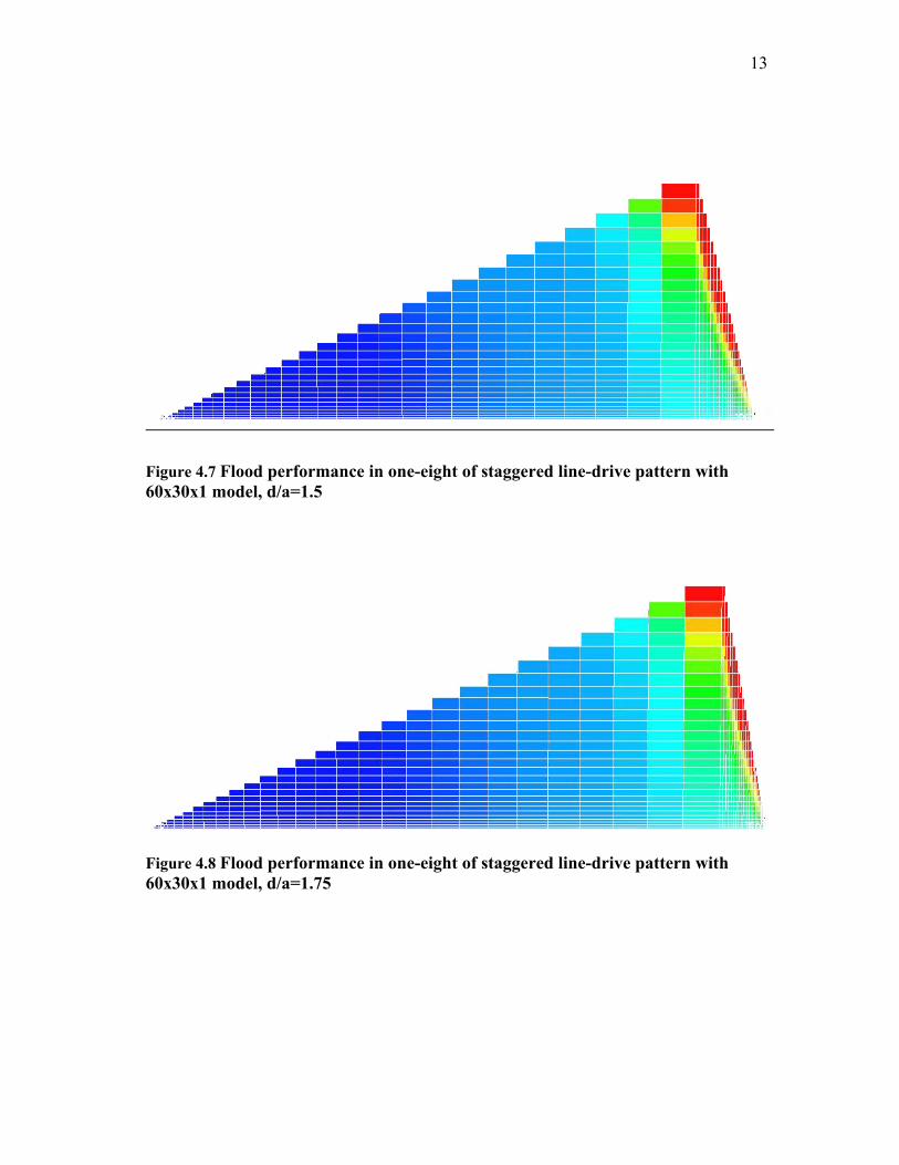
Fig. 4.4 through Fig. 4.8 represent staggered patterns performance at breakthrough

for finest grid distribution (60x30x1), where aspect ratio is changing from 0.75 to 1.75.

10

Figure 4.1 Flood performance in one-eight of five-spot pattern with 20x10x1 model


11


Figure 4.4 Flood performance in one-eight of staggered line-drive pattern with 60x30x1model, d/a=0.75

12

Figure 4.5 Flood performance in one-eight of staggered line-drive pattern with 60x30x1 model, d/a=1

Figure 4.6 Flood performance in one-eight of staggered line-drive pattern with 60x30x1 model, d/a=1.25

13



14

4.3 Methodology

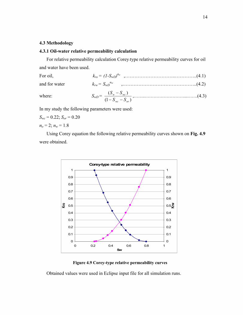
4.3.1 Oil-water relative permeability calculation

For relative permeability calculation Corey-type relative permeability curves for oil

and water have been used.

For oil, kro = (1-SwD)no ,…………………………..…………..(4.1)

and for water krw = SwDnw ,………………………………………..(4.2)

where: SwD = )1(

)(

orwc

wcw

SS

SS

,……..………………………...…….(4.3)

In my study the following parameters were used:

Swc = 0.22; Sor = 0.20

no = 2; nw = 1.8

Using Corey equation the following relative permeability curves shown on Fig. 4.9

were obtained.

Corey-type relative permeability

0

0.1

0.2

0.3

0.4

0.5

0.6

0.7

0.8

0.9

1

0 0.2 0.4 0.6 0.8 1Sw

Kro

0

0.1

0.2

0.3

0.4

0.5

0.6

0.7

0.8

0.9

1K

rw

Figure 4.9 Corey-type relative permeability curves

Obtained values were used in Eclipse input file for all simulation runs.

15

4.3.2 Fractional flow calculations

In a waterflood in which there is no saturation gradient behind the waterflood front,

there is no ambiguity about the value of water relative permeability to be used.

However, in my research in which there is a saturation gradient behind the flood front,

how can we select the appropriate value of water relative permeability?

Some of the early experimental results avoided that question by the use of flow

models with miscible fluids in which there is no saturation gradient behind the injected

fluid front. In 1955, Craig et al. presented the results of waterflood model in five-spot

pattern. A variety of oil viscosities used to obtain a range of saturation gradients and it

was found that if the water mobility was defined at the average water saturation behind

the flood front at water breakthrough, the data on areal sweep versus mobility ratio

would match those obtained by using miscible fluids. As a result of those studies, the

water mobility is defined as that at the average water saturation in the water-contacted

portion of the reservoir and this definition has been widely accepted.3

After obtaining relative permeabilities for oil and water, the fractional flow curves

for each viscosity ratio µo/µw is to be found. Using the definition of fractional flow,

fw =

o

w

µ

µ1

1

ro

rw

k

k

,…………….….……………………… (4.4)

By substituting for kro and krw from Eqs. 3.1 and 3.2, we can build charts (Fig. 4.10

through Fig. 4.13) that help us to obtain average water saturation behind flood front Sw

for each corresponding µo/µw ratio.

16

Figure 4.10 Fractional flow curves for µo/µw ratio equal 0.2 and 0.5

µo/µw = 0.2

0

0.1

0.2

0.3

0.4

0.5

0.6

0.7

0.8

0.9

1

0 0.1 0.2 0.3 0.4 0.5 0.6 0.7 0.8 0.9

Sw

fw

µo/µw = 0.5

0

0.1

0.2

0.3

0.4

0.5

0.6

0.7

0.8

0.9

1

0 0.1 0.2 0.3 0.4 0.5 0.6 0.7 0.8 0.9

Sw

fw

17

Figure 4.11 Fractional flow curves for µo/µw ratio equal 1 and 2

µo/µw = 2

0

0.1

0.2

0.3

0.4

0.5

0.6

0.7

0.8

0.9

1

0 0.1 0.2 0.3 0.4 0.5 0.6 0.7 0.8 0.9

Sw

fwµo/µw = 1

0

0.1

0.2

0.3

0.4

0.5

0.6

0.7

0.8

0.9

1

0 0.1 0.2 0.3 0.4 0.5 0.6 0.7 0.8 0.9

Sw

fw

18

Figure 4.12 Fractional flow curves for µo/µw ratio equal 3 and 5

µo/µw = 3

0

0.1

0.2

0.3

0.4

0.5

0.6

0.7

0.8

0.9

1

0 0.1 0.2 0.3 0.4 0.5 0.6 0.7 0.8 0.9

Sw

fw

µo/µw = 5

0

0.1

0.2

0.3

0.4

0.5

0.6

0.7

0.8

0.9

1

0 0.1 0.2 0.3 0.4 0.5 0.6 0.7 0.8 0.9

Sw

fw

19

Figure 4.13 Fractional flow curve for µo/µw ratio equal 10

To find Sw value we needed to the know exact point of the intersection of the

tangent of the fractional flow curve with the maximum water fraction that equals 1,

then simply by drawing a line from that intersection to Sw scale we obtain the average

water saturation behind the water front for each µo/µw case:

µo/µw =0.2; Sw = 0.77

µo/µw =0.5; Sw = 0.74

µo/µw =1; Sw = 0.7

µo/µw =2; Sw = 0.635

µo/µw =3; Sw = 0.6

µo/µw =5; Sw = 0.53

µo/µw =10; Sw = 0.45

µo/µw = 10

0

0.1

0.2

0.3

0.4

0.5

0.6

0.7

0.8

0.9

1

0 0.1 0.2 0.3 0.4 0.5 0.6 0.7 0.8 0.9

Sw

fw

20

4.3.3 Mobility ratio calculation

We will use these values to calculate the end point water relative permeability rwek

for each viscosity ratio by applying Eq. 4.2 and substituting Sw on the obtained Sw in

Eq. 4.3. Then using Eq. 1.2 we can estimate the mobility ratio M, calculated values

presented in Table 4.1.

Table 4.1

µo/µw Sw Krwe M0.2 0.77 0.909 0.1820.5 0.74 0.822 0.4111 0.7 0.711 0.7112 0.635 0.547 1.0953 0.6 0.467 1.4015 0.53 0.324 1.619

10 0.45 0.189 1.892

4.3.4 Breakthrough determination

In the following sections I presented calculations that correspond to a five-spot

waterflood pattern with finest 60x30x1model, similar methodology can be used for all

other models and patterns. Fractional flow at the producer versus displacing fluid

injected obtained from the simulation output file (RSM) where fw is water fraction at

the producer and WiD is dimensionless value of water injected at injector.

WiD = )1(

*0.000129

orwc

i

SSAh

W

,……………...……...………..(4.5)

Where Wi is cumulative water injected at certain time, A is for grid block area

which in our case equal 40 acres, h is 20 ft. and φ equal 0.3 for total porosity.

21

Figure 4.14 Fractional flow fw versus WiD for viscosity ratios µo/µw equal 0.2 and 0.5

µo/µw=0.2

0

0.05

0.1

0.15

0.2

0.25

0.3

0.35

0.4

0.45

0.5

0 0.1 0.2 0.3 0.4 0.5 0.6 0.7 0.8 0.9 1

WiD

f w

µo/µw=0.5

0

0.05

0.1

0.15

0.2

0.25

0.3

0.35

0.4

0.45

0.5

0 0.1 0.2 0.3 0.4 0.5 0.6 0.7 0.8 0.9 1WiD

f w

22

Figure 4.15 Fractional flow fw versus WiD for viscosity ratios µo/µw equal 1 and 2

µo/µw=1

0

0.05

0.1

0.15

0.2

0.25

0.3

0.35

0.4

0.45

0.5

0 0.1 0.2 0.3 0.4 0.5 0.6 0.7 0.8 0.9 1WiD

f w

µo/µw=2

0

0.05

0.1

0.15

0.2

0.25

0.3

0.35

0.4

0.45

0.5

0 0.1 0.2 0.3 0.4 0.5 0.6 0.7 0.8 0.9 1WiD

f w

23

Figure 4.16 Fractional flow fw versus WiD for viscosity ratios µo/µw equal 3 and 5

µo/µw=3

0

0.05

0.1

0.15

0.2

0.25

0.3

0.35

0.4

0.45

0.5

0 0.1 0.2 0.3 0.4 0.5 0.6 0.7 0.8 0.9 1WiD

fw

µo/µw=5

0

0.05

0.1

0.15

0.2

0.25

0.3

0.35

0.4

0.45

0.5

0 0.1 0.2 0.3 0.4 0.5 0.6 0.7 0.8 0.9 1WiD

f w

24

µo/µw=10

0

0.05

0.1

0.15

0.2

0.25

0.3

0.35

0.4

0.45

0.5

0 0.1 0.2 0.3 0.4 0.5 0.6 0.7 0.8 0.9 1

WiD

fw

Figure 4.17 Fractional flow fw versus WiD for viscosity ratio µo/µw equal 10

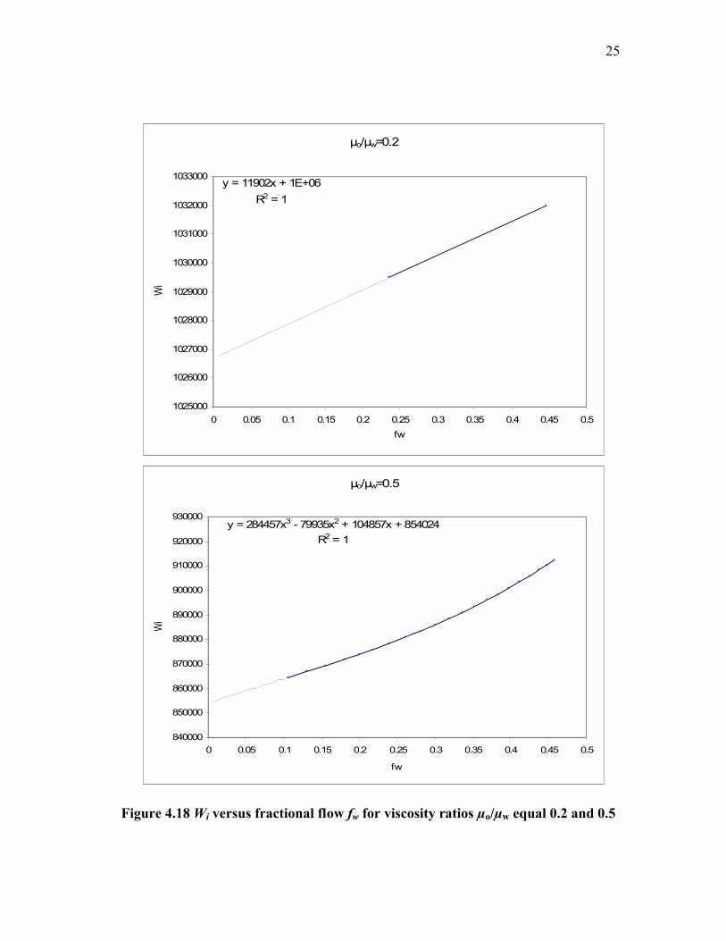
Due to numerical dispersion of simulation, injected fluid breaks through earlier at

the producer than it should. The fractional flow versus WiD plots shown in Fig. 4.14

through Fig. 4.17 illustrate the early breakthrough caused by numerical dispersion.

To correct for numerical dispersion in breakthrough times and approximate the

breakthrough time more accurately, we use fractional flow data after breakthrough and

extrapolate back to breakthrough time. A third order polynomial is used for this method

except for case when µo/µw is equal 0.2 (second order used to get smaller divergence).

Microsoft Excel build-in trend line function were used obtain the polynomial fits

presented in charts in Fig. 4.18 through Fig. 4.21.

Wi = afw3+bfw

2+cfw+d,……….…………………..……(4.6)

25

Figure 4.18 Wi versus fractional flow fw for viscosity ratios µo/µw equal 0.2 and 0.5

µo/µw=0.2

y = 11902x + 1E+06

R2 = 1

1025000

1026000

1027000

1028000

1029000

1030000

1031000

1032000

1033000

0 0.05 0.1 0.15 0.2 0.25 0.3 0.35 0.4 0.45 0.5

fw

Wi

µo/µw=0.5

y = 284457x3 - 79935x2 + 104857x + 854024

R2 = 1

840000

850000

860000

870000

880000

890000

900000

910000

920000

930000

0 0.05 0.1 0.15 0.2 0.25 0.3 0.35 0.4 0.45 0.5

fw

Wi

26

Figure 4.19 Wi versus fractional flow fw for viscosity ratios µo/µw equal 1 and 2

µo/µw=1

y = 608249x3 - 157232x2 + 186008x + 696216

R2 = 1

600000

650000

700000

750000

800000

850000

900000

0 0.1 0.2 0.3 0.4 0.5 0.6

fw

Wi

µo/µw=2

y = 726364x3 - 126537x2 + 220423x + 542525

R2 = 1

500000

550000

600000

650000

700000

750000

800000

0 0.1 0.2 0.3 0.4 0.5 0.6

fw

Wi

27

Figure 4.20 Wi versus fractional flow fw for viscosity ratios µo/µw equal 3 and 5

µo/µw=3

y = 802613x3 - 121830x2 + 223638x + 460751

R2 = 1

400000

450000

500000

550000

600000

650000

700000

0 0.1 0.2 0.3 0.4 0.5 0.6

fw

Wi

µo/µw=5

y = 1E+06x3 - 403689x2 + 302525x + 361529

R2 = 1

300000

350000

400000

450000

500000

550000

600000

0 0.1 0.2 0.3 0.4 0.5 0.6

fw

Wi

28

µo/µw=10

y = 1E+06x3 - 498312x2 + 336639x + 250540

R2 = 1

200000

250000

300000

350000

400000

450000

500000

0 0.1 0.2 0.3 0.4 0.5 0.6

fw

Wi

Figure 4.21 Wi versus fractional flow fw for viscosity ratio µo/µw equal 10

From Eq. 3.6 we use “d” coefficient as a value of cumulative water injected at

breakthrough because with this value polynomial equations intersect Wi scale, that tells

us very accurately when water fraction fw begin to appear (breakthrough). Then, simply

using Eq. 1.5 and applying obtained Wi values we estimate areal sweep efficiency for

each defined mobility ratio.

29

CHAPTER V

SIMULATION RESULTS

Finally, I made simulation runs and determined areal sweep efficiencies at

breakthrough for other grid block dimensions and staggered line drive patterns with

various aspect ratios. These are described below.

Fig. 5.1 graphically presents simulated results for 40x20x1 model and experimental

results obtained in different time by different investigators. It shows very good

agreement between these models, however for mobility ratios greater than 1 (M>1) we

can notice that simulation areal sweep efficiency begins to decrease much faster than it

is for experiments.

For 60x30x1 grid model illustrated in comparison with experimental results in Fig.

5.2, there is greater deviation in simulation areal sweep efficiency results than it is for

40x20x1 model, but considering areal sweep efficiency values for M>1 we see much

better alignment with experimental results. This advantage lets us use a larger range of

mobility ratios for pattern behavior investigation.

Fig. 5.3 represents all simulation results performed for the five spot pattern, this

will help us to better understand the effect of grid block number on simulation results.

In this figure, I also presented simulation results for 20x10x1 and 200x100x1 models.

From the chart it is easy noticeable that 20x10x1 model has worse alignment with

experiments as well as performance for unfavorable mobility ratios (M>1), this leads us

to eliminate this model from further study of staggered line drive patterns behavior.

Additional 200x100x1 grid block model used to better represent the effect of grid block

number on simulation results and its reliability.

30

Five-Spot Pattern Bebavior

0.4

0.5

0.6

0.7

0.8

0.9

1

0.1 1 10Mobility Ratio

Are

al S

we

ep

Effi

cie

ncy

......

.

Eclipse Simulation

Craig, Geffen and Morse 1955

Dyes, Caudle and Erickson 1954

Figure 5.1 Comparison of Eclipse simulation results for 40x20x1 model with experimental values in five-spot waterflood pattern

31

Five-Spot Pattern Bebavior

0.4

0.5

0.6

0.7

0.8

0.9

1


Are

al S

we

ep

Effi

cie

ncy

......

.

Eclipse Simulation

Craig, Geffen and Morse 1955

Dyes, Caudle and Erickson 1954

Figure 5.2 Comparison of Eclipse simulation results for 60x30x1 model with experimental values in five-spot waterflood pattern

32

Five-Spot Pattern Behavior

0.3

0.4

0.5

0.6

0.7

0.8

0.9

1


Area

l Sw

eep

Effic

ienc

y

Craig's model

60x30x1 model

40x20x1 model

20x10x1 model

200x100x1 model

Figure 5.3 Illustration and comparison of five-spot pattern behavior for different grid models with Craig model

33

Staggered Line Drive Patterns Behavior

0.4

0.5

0.6

0.7

0.8

0.9

1


Are

al S

wee

p E

ffici

ency

......

.

d/a=0.75

d/a=1

d/a=1.25

d/a=1.5

d/a=1.75

Dyes d/a=1

Figure 5.4 Comparison of 40x20x1 staggered line drive patterns simulation results for different aspect ratios (d/a) with Dyes experimental values for d/a=1

34

Staggered Line Drive Patterns Behavior

0.5

0.6

0.7

0.8

0.9

1


Area

l Sw

eep

Effic

ienc

y....

.. .

d/a=0.75

d/a=1

d/a=1.25

d/a=1.5

d/a=1.75

Dyes d/a=1

Figure 5.5 Comparison of 60x30x1 staggered line drive patterns simulation results for different aspect ratios (d/a) with Dyes experimental values for d/a=1

35

Fig. 5.4 shows staggered line drive pattern performance for different aspect ratios

performed in 40x20x1 simulation model. Results compared against the Dyes

experimental values for aspect ratio d/a = 1. We can see poor agreement between

simulation and experimental values for areal sweep efficiencies may caused by

relatively small grid block number (40x20x1).

Next chart (Fig. 5.5) presents the same results only for 60x30x1 grid block model.

Here we can notice large improvement in terms of alignment. Best agreement between

simulation results and experimental occurs approximately in 0.4-0.6 mobility ratio

range where the affect of aspect ratio on areal sweep is negligible.

In the following graphs (Fig. 5.6 and Fig. 5.7) I showed the obtained results in

representation of flood efficiencies for unit mobility ratio (M = 1), where we study the

effect of aspect ratio (d/a) on pattern performance. Results of two models 40x20x1 and

60x30x1in each chart compared with experimental results obtained by different

investigators. After comparing the simulation results of the first model (40x20x1) with

Muskat’s values we can set the deviation range that vary from 0.08 to 0.16 of areal

sweep efficiency, for second (60x30x1) it is from 0.04 to 0.08.

Again, for 40x20x1 model it is clear that agreement with experiments is worse than

it is for another (60x30x1) not only considering wider deviation range but also because

of reverse curve’s trend i.e. areal sweep efficiency decrease with increase of aspect

ratio.

Thus after summarizing the facts concluded from presented results, the simulation

model that gives the most satisfactory match with experimental data is the 60x30x1

model.

36

Flooding Efficiency

0.4

0.6

0.8

1

0.4 0.8 1.2 1.6 2

Aspect Ratio d/a

Are

al S

wee

p E

ffici

ency

Eclipse Simulator

Muskat 1950

Prats 1956

Figure 5.6 Comparison of 40x20x1 model’s flood efficiency for unit mobility ratio (M=1)

Flooding Efficiency

0.4

0.6

0.8

1

0.4 0.8 1.2 1.6 2

Aspect Ratio d/a

Are

al S

wee

p E

ffici

ency

Eclipse Simulator

Muskat 1950

Prats 1956

Figure 5.7 Comparison of 60x30x1 model’s flood efficiency for unit mobility ratio (M=1)

37

CHAPTER VI

SUMMARY, CONCLUSIONS AND RECOMMENDATIONS

6.1 Summary

A simulation study has been performed with the main objective of determining the

areal sweep efficiency at breakthrough for waterflood staggered line drive as a function

of the Craig mobility ratio for a range of aspect ratios. The two-dimensional simulation

model represents 1/8 of a 40-acre pattern unit with a reservoir thickness of 20 ft.

Simulation runs using a number of Cartesian grid models were made to determine the

optimum grid model. The Cartesian models tested were 20x10x1, 40x20x1, 60x30x1

and 200x100x1. The simulation results of areal sweep efficiency versus mobility ratio

were compared against available experimental data for 5-spot pattern and staggered line

drive with aspect ratio of 1. The simulation model that gave the most satisfactory

match with experimental data was the 60x30x1 model and therefore was selected for

detailed study.

6.2 Conclusions

The main conclusion of the simulation study may be summarized as follows:

1. For staggered line drive patterns, simulation results are in very satisfactory

agreement with experimental data for water-oil mobility ratio in the range, 0.4-0.6,

where the affect of staggered line drive aspect ratio on areal sweep at breakthrough is

not significant. For mobility ratio above 0.6 and aspect ratio of 1, the areal sweep

efficiency at breakthrough shows a slightly higher trend compared to simulation data

(for example, 0.72 versus 0.75 at mobility ratio of 1. For mobility ratio less than 0.4,

the simulated areal sweep efficiency is slightly higher than the experimental data (for

example, 0.93 versus 0.88 at mobility ratio of 0.2).

2. Areal sweep efficiency decreases with an increase in mobility ratio – in line with

experimental data - for all aspect ratios. These results clearly indicate that water-oil

mobility ratio controls the displacement of oil by water at the pore level.

3. Areal sweep efficiency increases with an increase in aspect ratio (for mobility ratios

greater than 0.5) – in line with experimental data. The results underscore the fact that

38

the aspect ratio in a staggered line drive controls the displacement of oil by water at the

macro level.

4. A major problem encountered during the study is the determination of breakthrough

time. This problem has been reported by others doing similar type of research. The

main cause of the problem is probably numerical dispersion, although just increasing

the number of grid blocks in the model does not seem to completely eliminate the

problem.

6.3 Recommendations

The following recommendations are suggested for future research:

1. The simulation study indicates the importance of choosing an optimal number of grid

blocks in a simulation model, so as to obtain minimum dispersion yet not to have a too

large a model that will take too long to run.

2. For future studies, it is suggested to limit the mobility ratio range to about 0.2 to 1.5,

to avoid discrepancy (stemming from numerical dispersion) with experimental results.

3. It is recommended to investigate the possibility of minimizing or eliminating the

numerical dispersion problem by, for instance, the use of streamline simulation.

39

NOMENCLATURE

AS area swept, sqft

AT total area of the pattern, sqft

a distance between like wells (injection or production) in a row, ft

d distance between adjacent rows of injection and production wells, ft

EA areal sweep efficiency

fw fractional flow of water

h bed thickness, ft

k permeability, mD

kro relative permeability of oil

krw relative permeability of water

M mobility ratio

porosity

viscosity,cp

Wi volume of displacing phase injected,

40

REFERENCES

Brigham, William E., Kovscek, Anthony R., Wang, Y. 1998. A Study of the Effect of

Mobility Ratios on Pattern Displacement Behavior and Streamline to infer Permeability

Fields Permeability Media. MS thesis, SUPRI-A.

Craig, F. F. Jr. 1971. The Reservoir Engineering Aspect of Water Flooding. SPE

Monograph, Vol. 3.

Dyes, A.B., Caudle B.H., and Erickson R.A.1954. Oil Production after Breakthrough –

as Influenced by Mobility Ratio. Petroleum Trans. AIME, 201: 27-32.

Morel-Seytoux, H.J., 1966. Unit Mobility Ratio Displacement Calculations for Pattern

Floods in Homogeneous Medium. SPE, 6: 217-227.

Peaceman, D.W. 1977. Fundamentals of Numerical Reservoir Simulation. New York:

Elsevier Scientific Publishing Co.

Pitts, Gerald N., Crawford, Paul B. 1971. Simulating Large Flow Networks in

Underground Media. New York, ACM.

Prats, M. 1956. The Breakthrough Sweep Efficiency of the Staggered Line Drive.

Trans. AIME, 207: 67-68.

Willhite, G.P. 1986. Waterflooding. SPE Textbook Series Vol. 3. Richardson, Texas,

SPE.

41

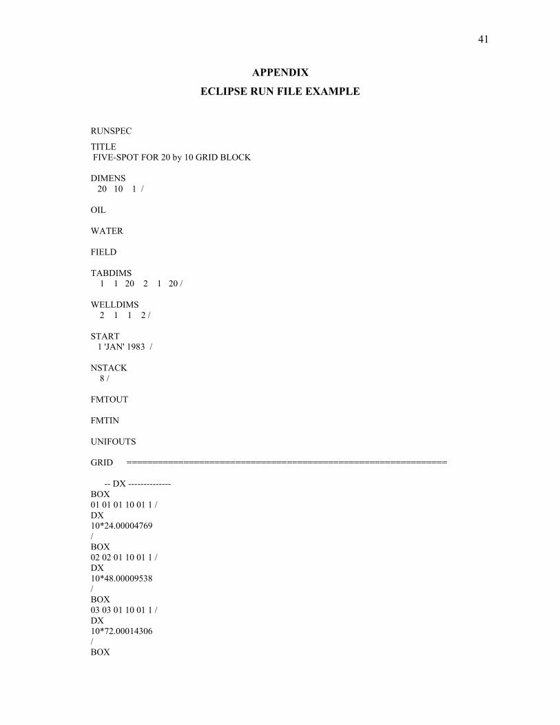
APPENDIX

ECLIPSE RUN FILE EXAMPLE

RUNSPEC

TITLE FIVE-SPOT FOR 20 by 10 GRID BLOCK

DIMENS 20 10 1 /

OIL

WATER

FIELD

TABDIMS 1 1 20 2 1 20 /

WELLDIMS 2 1 1 2 /

START 1 'JAN' 1983 /

NSTACK 8 /

FMTOUT

FMTIN

UNIFOUTS

GRID ==============================================================

-- DX --------------BOX01 01 01 10 01 1 /DX10*24.00004769/BOX02 02 01 10 01 1 /DX10*48.00009538/BOX03 03 01 10 01 1 /DX10*72.00014306/BOX

42

04 04 01 10 01 1 /DX10*96.00019075/BOX05 05 01 10 01 1 /DX10*120.0002384/BOX06 06 01 10 01 1 /DX10*144.0002861/BOX07 07 01 10 01 1 /DX10*168.0003338/BOX08 08 01 10 01 1 /DX10*192.0003815/BOX09 09 01 10 01 1 /DX10*216.0004292/BOX10 10 01 10 01 1 /DX10*240.0004769/BOX11 11 01 10 01 1 /DX10*240.0004769/BOX12 12 01 10 01 1 /DX10*216.0004292/BOX13 13 01 10 01 1 /DX10*192.0003815/BOX14 14 01 10 01 1 /DX10*168.0003338/BOX15 15 01 10 01 1 /

43

DX10*144.0002861/BOX16 16 01 10 01 1 /DX10*120.0002384/BOX17 17 01 10 01 1 /DX10*96.00019075/BOX18 18 01 10 01 1 /DX10*72.00014306/BOX19 19 01 10 01 1 /DX10*48.00009538/BOX20 20 01 10 01 1 /DX10*24.00004769/ENDBOX

-- DY ========================BOX01 20 01 01 01 1 /DY20*24.00004769/BOX01 20 02 02 01 1 /DY20*48.00009538/BOX01 20 03 03 01 1 /DY20*72.00014306/BOX01 20 04 04 01 1 /DY20*96.00019075/BOX01 20 05 05 01 1 /DY20*120.0002384/

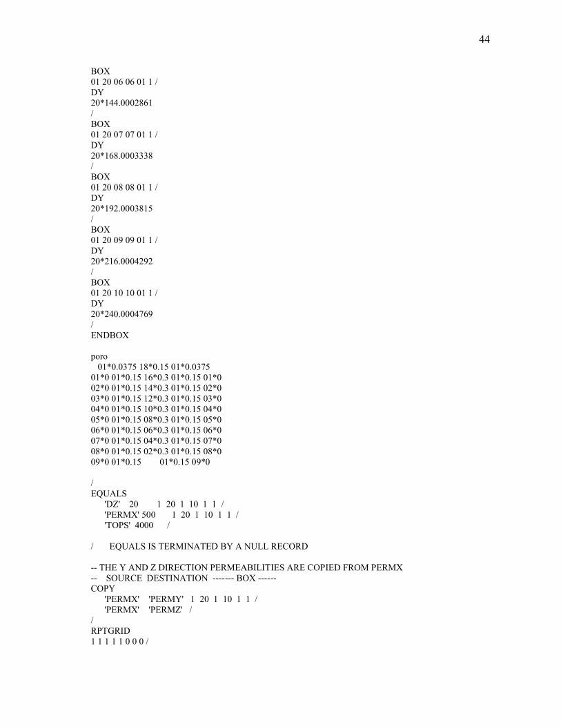
44

BOX01 20 06 06 01 1 /DY20*144.0002861/BOX01 20 07 07 01 1 /DY20*168.0003338/BOX01 20 08 08 01 1 /DY20*192.0003815/BOX01 20 09 09 01 1 /DY20*216.0004292/BOX01 20 10 10 01 1 /DY20*240.0004769/ENDBOX

poro 01*0.0375 18*0.15 01*0.037501*0 01*0.15 16*0.3 01*0.15 01*002*0 01*0.15 14*0.3 01*0.15 02*003*0 01*0.15 12*0.3 01*0.15 03*004*0 01*0.15 10*0.3 01*0.15 04*005*0 01*0.15 08*0.3 01*0.15 05*006*0 01*0.15 06*0.3 01*0.15 06*007*0 01*0.15 04*0.3 01*0.15 07*008*0 01*0.15 02*0.3 01*0.15 08*009*0 01*0.15 01*0.15 09*0

/EQUALS 'DZ' 20 1 20 1 10 1 1 / 'PERMX' 500 1 20 1 10 1 1 / 'TOPS' 4000 /

/ EQUALS IS TERMINATED BY A NULL RECORD

-- THE Y AND Z DIRECTION PERMEABILITIES ARE COPIED FROM PERMX-- SOURCE DESTINATION ------- BOX ------COPY 'PERMX' 'PERMY' 1 20 1 10 1 1 / 'PERMX' 'PERMZ' //RPTGRID1 1 1 1 1 0 0 0 /

45

DEBUG 0 0 1 0 1 0 1 /

PROPS ==============================================================

SWFN 0.22 .0 0 0.24 .002332 0 0.32 .04225 0 0.37 .087658 0 0.42 .147124 0 0.52 .305245 0 0.57 .402858 0 0.62 .512316 0 0.72 .765554 0 0.8 1 0/SOF2 1 TABLES 20 NODES IN EACH FIELD 13:34 5 MAY 85 .20 .0000 .28 .019025 .38 .096314 .43 .157253 .48 .233056 .58 .429251 .63 .549643 .68 .684899 .76 .932224 .78 1/

PVTW .0 1.0 3.03E-06 1 0.0 /

PVDO .0 1.0 1 8000.0 .92 1/ROCK 4000.0 .30E-05 /

DENSITY 52.0000 64.0000 .04400 /

RPTPROPS 2*0 /

REGIONS =============================================================

SATNUM 200*1 /

SOLUTION =============================================================

EQUIL4000 4000 6000 0 0 0 0 0 0 /

46

RPTSOL1 0 1 /

SUMMARY ===========================================================

--REQUEST PRINTED OUTPUT OF SUMMARY FILE DATA

WOPR/WWPR/WWCT/WWIT/

RUNSUM

SEPARATE

RPTSMRY 1 /

SCHEDULE ===========================================================

TUNING10 25 /1.0 0.5 1.0E-6 //WELSPECS'INJECTOR' 'G' 20 1 4000 'water' /'PRODUCER' 'G' 1 1 4000 'OIL' //COMPDAT'INJECTOR' 20 1 1 1 'OPEN' 0 .0 0.5 /'PRODUCER' 1 1 1 1 'OPEN' 0 .0 0.5 //WCONPROD'PRODUCER' 'OPEN' 'lRAT' 1* 1* 1* 100 1* 1* //WCONINJE'INJECTOR' 'WAT' 'OPEN' 'RATE' 100 //TSTEP20*365/

END

47

VITA

Name: Ruslan Guliyev

Address: Department of Petroleum Engineering

Texas A&M University

College Station, TX 77843-3116

Email Address: [email protected]

Education: B.S., Petroleum Engineering, Azerbaijan State Oil

Academy, 2002.

M.S., Petroleum Engineering, Texas A&M

University, 2008.

Employment History: Schlumberger, Wireline Engineer, CAG, 2002-2004

Internship in BP Azerbaijan, Azeri Base

Management Team. 2005.

simulation study of areal sweep efficiency...

Documents