Simulation with Matlab

Professor Nhut Tan Ho

ME584

simmat 1

Agenda

• Representations of dynamic systems

• Simulation of

– Linear systems

– Non-linear systems

• Active learning activities: pair-share exercises

simmat 2

Representation of Dynamic Systems

simmat 3

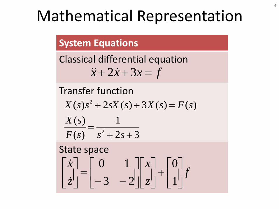
Mathematical Representation

simmat

4

System Equations

Classical differential equation

Transfer function

State space

fxxx 32

32

1

)(

)(

)()(3)(2)(

2

2

sssF

sX

sFsXssXssX

fz

x

z

x

1

0

23

10

Finding Roots of Polynomial

simmat 5

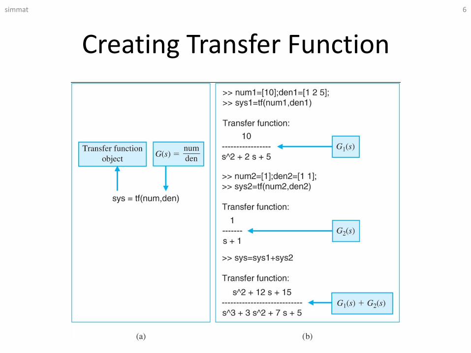
Creating Transfer Function

simmat 6

ss function and model conversion

simmat 7

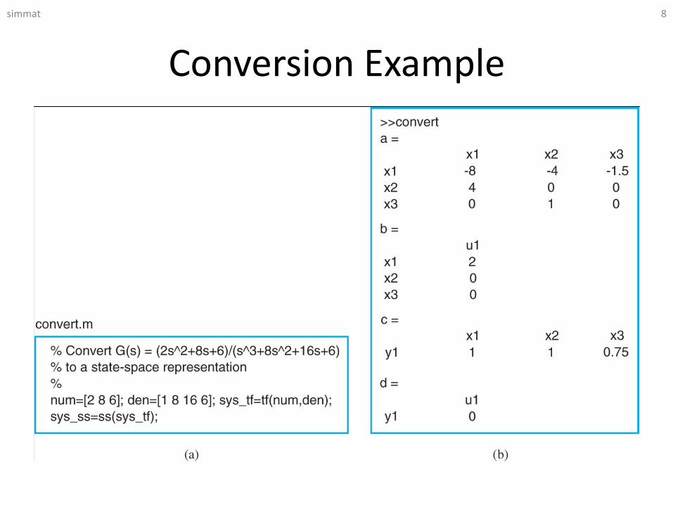
Conversion Example

simmat 8

Roots of Characteristic Polynomialsimmat 9

Simulation of Linear Systems

simmat 10

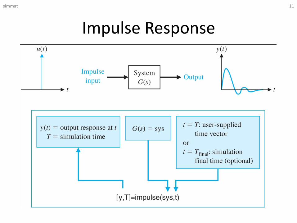
Impulse Response

simmat 11

Impulse Example

Second order system

ωn=1

simmat 12

Step Function

simmat 13

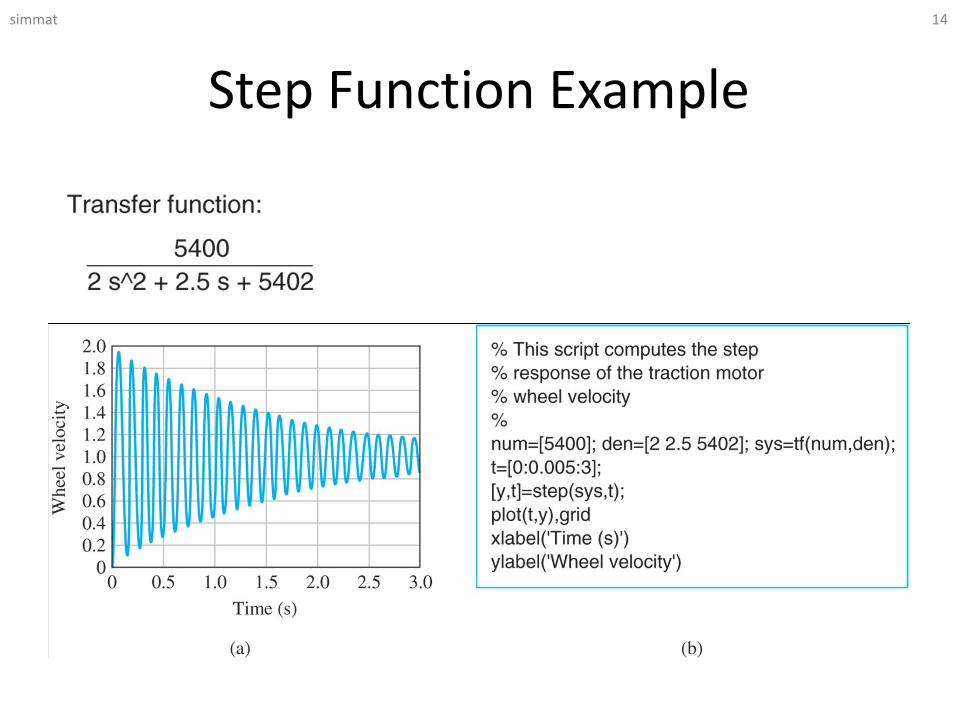
Step Function Example

simmat 14

lsim function

simmat 15

lsim examplesimmat 16

Simulation of Nonlinear Systems

simmat 17

ODE Solvers

simmat 18

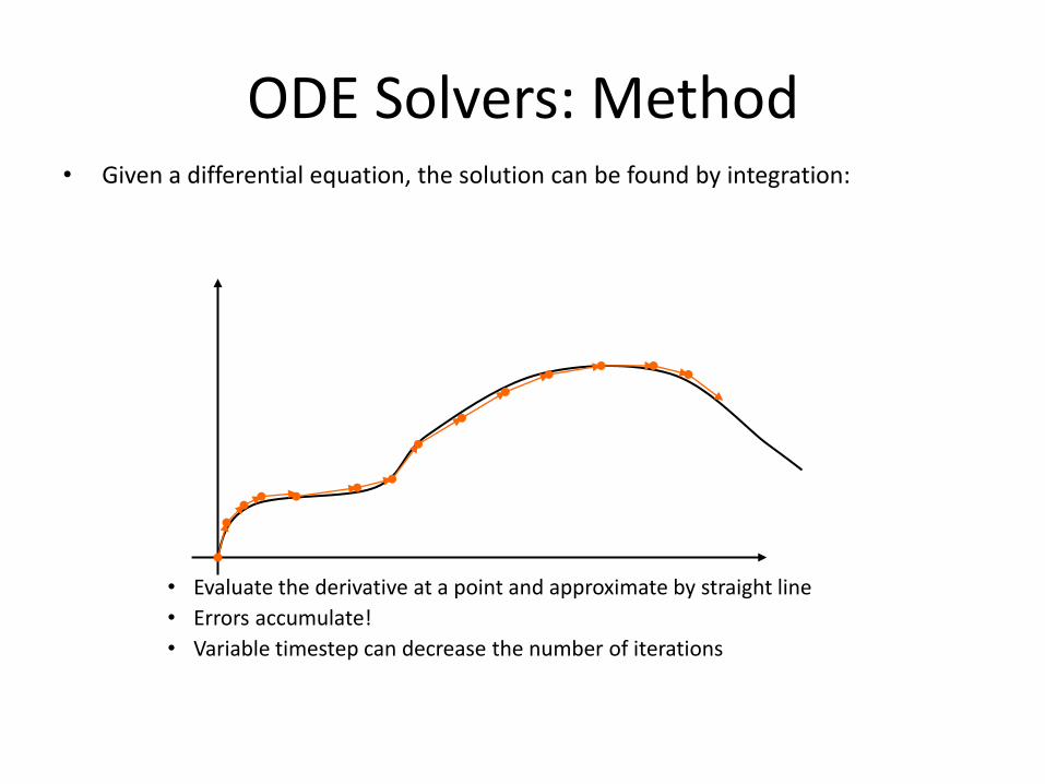
ODE Solvers: Method• Given a differential equation, the solution can be found by integration:

• Evaluate the derivative at a point and approximate by straight line

• Errors accumulate!

• Variable timestep can decrease the number of iterations

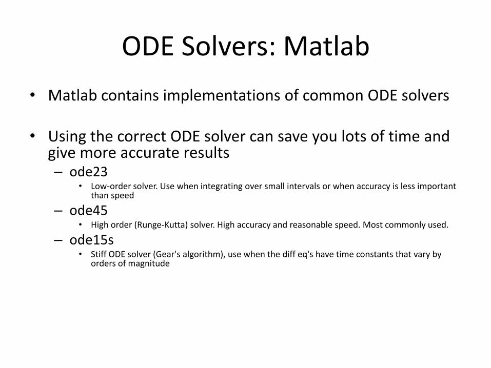
ODE Solvers: Matlab

• Matlab contains implementations of common ODE solvers

• Using the correct ODE solver can save you lots of time and give more accurate results– ode23

• Low-order solver. Use when integrating over small intervals or when accuracy is less important than speed

– ode45• High order (Runge-Kutta) solver. High accuracy and reasonable speed. Most commonly used.

– ode15s• Stiff ODE solver (Gear's algorithm), use when the diff eq's have time constants that vary by

orders of magnitude

ODE Solvers: Standard Syntax

• To use standard options and variable time step– [t,y]=ode45('myODE',[0,10],[1;0])

• Inputs:• ODE function name (or anonymous function). This function takes inputs (t,y),

and returns dy/dt• Time interval: 2-element vector specifying initial and final time• Initial conditions: column vector with an initial condition for each ODE. This is

the first input to the ODE function

• Outputs:• t contains the time points• y contains the corresponding values of the integrated variables.

ODE integrator: 23, 45, 15s

ODE function Time range

Initial conditions

ODE Function• The ODE function must return the value of the

derivative at a given time and function value

• Example: chemical reaction• Two equations

• ODE file:

– y has [A;B]

– dydt has[dA/dt;dB/dt]

A B

10

5010 50

10 50

dAA B

dt

dBA B

dt

ODE Function: viewing results

• To solve and plot the ODEs on the previous slide:– [t,y]=ode45('chem',[0 0.5],[0 1]);

• assumes that only chemical B exists initially

– plot(t,y(:,1),'k','LineWidth',1.5);

– hold on;

– plot(t,y(:,2),'r','LineWidth',1.5);

– legend('A','B');

– xlabel('Time (s)');

– ylabel('Amount of chemical (g)');

– title('Chem reaction');

ODE Function: viewing results• The code on the previous slide produces this figure

0 0.05 0.1 0.15 0.2 0.25 0.3 0.35 0.4 0.45 0.50

0.1

0.2

0.3

0.4

0.5

0.6

0.7

0.8

0.9

1

Time (s)

Am

ount

of

chem

ical (g

)

Chem reaction

A

B

Higher Order Equations• Must make into a system of first-order equations to use ODE

solvers

• Nonlinear is OK!

• Pendulum example:

0g

sinL

gsin

L

let

gsin

L

x

dx

dt

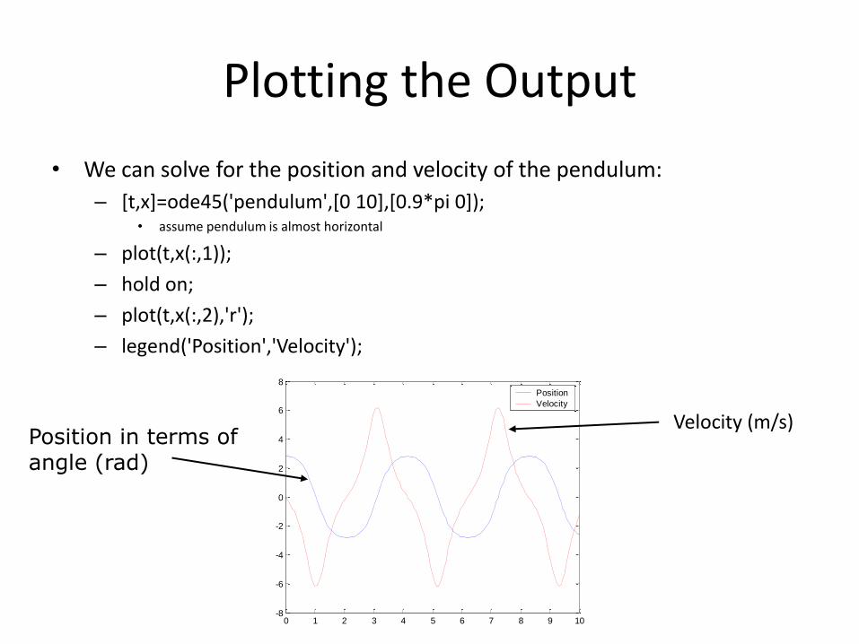
Plotting the Output

• We can solve for the position and velocity of the pendulum:

– [t,x]=ode45('pendulum',[0 10],[0.9*pi 0]);• assume pendulum is almost horizontal

– plot(t,x(:,1));

– hold on;

– plot(t,x(:,2),'r');

– legend('Position','Velocity');

0 1 2 3 4 5 6 7 8 9 10-8

-6

-4

-2

0

2

4

6

8

Position

Velocity

Position in terms ofangle (rad)

Velocity (m/s)

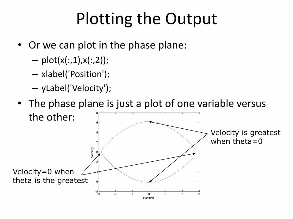
Plotting the Output

• Or we can plot in the phase plane:

– plot(x(:,1),x(:,2));

– xlabel('Position');

– yLabel('Velocity');

• The phase plane is just a plot of one variable versus the other:

-3 -2 -1 0 1 2 3-8

-6

-4

-2

0

2

4

6

8

Position

Velo

city

Velocity is greatest when theta=0

Velocity=0 when theta is the greatest

ODE Solvers: Custom Options• Matlab's ODE solvers use a variable timestep

• Sometimes a fixed timestep is desirable– [t,y]=ode45('chem',[0:0.001:0.5],[0 1]);

• Specify the timestep by giving a vector of times

• The function value will be returned at the specified points

• Fixed timestep is usually slower because function values are interpolated to give values at the desired timepoints

• You can customize the error tolerances using odeset– options=odeset('RelTol',1e-6,'AbsTol',1e-10);

– [t,y]=ode45('chem',[0 0.5],[0 1],options);• This guarantees that the error at each step is less than RelTol times the value at that

step, and less than AbsTol

• Decreasing error tolerance can considerably slow the solver

• See doc odeset for a list of options you can customize

Pair-Share Exercise: ODE

• Use ode45 to solve for on the range t=[0 10], with initial condition and

• Plot the result.

10dy dt t y

y t

0 10y

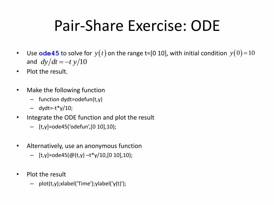
Pair-Share Exercise: ODE

• Use ode45 to solve for on the range t=[0 10], with initial condition and

• Plot the result.

• Make the following function

– function dydt=odefun(t,y)

– dydt=-t*y/10;

• Integrate the ODE function and plot the result

– [t,y+=ode45(‘odefun’,*0 10+,10);

• Alternatively, use an anonymous function

– [t,y]=ode45(@(t,y) –t*y/10,[0 10],10);

• Plot the result

– plot(t,y);xlabel('Time');ylabel('y(t)');

10dy dt t y y t 0 10y

Exercise: ODE

• The integrated function looks like this:

0 1 2 3 4 5 6 7 8 9 100

1

2

3

4

5

6

7

8

9

10

Time

y(t

)Function y(t), integrated by ode45

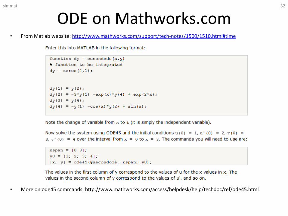
ODE on Mathworks.com• From Matlab website: http://www.mathworks.com/support/tech-notes/1500/1510.html#time

• More on ode45 commands: http://www.mathworks.com/access/helpdesk/help/techdoc/ref/ode45.html

simmat 32

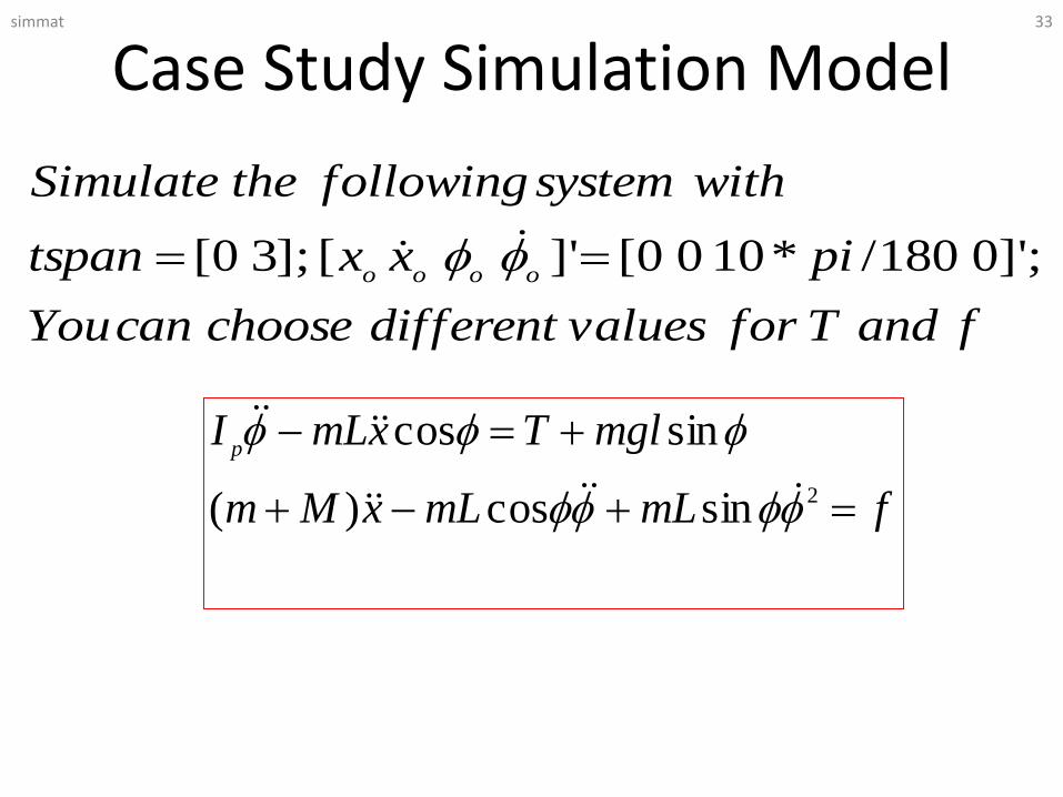
Case Study Simulation Modelsimmat 33

fmLmLxMm

mglTxmLIp

2sincos)(

sincos

fandTforvaluesdifferentchoosecanYou

pixxtspan

withsystemfollowingtheSimulate

oooo;]'0180/*1000[]'[];30[

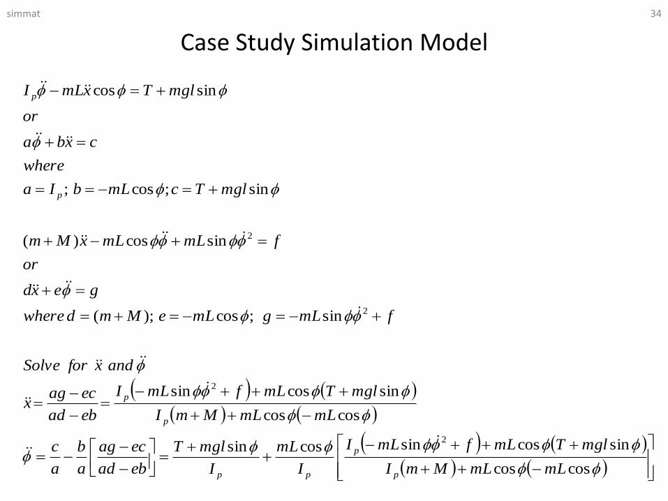
Case Study Simulation Model

simmat 34

coscos

sincossincossin

coscos

sincossin

sin;cos);(

sincos)(

sin;cos;

sincos

2

2

2

2

mLmLMmI

mglTmLfmLI

I

mL

I

mglT

ebad

ecag

a

b

a

c

mLmLMmI

mglTmLfmLI

ebad

ecagx

andxforSolve

fmLgmLeMmdwhere

gexd

or

fmLmLxMm

mglTcmLbIa

where

cxba

or

mglTxmLI

p

p

pp

p

p

p

p

Matlab Simulationsimmat 35

);**/()**(*)/(/)4(

);4()3(

);**/()**()2(

);2()1(

)]'4()3()2()1([]'[%

;)4(*)4(*))3(sin(**

));3(cos(**

);(

));3(sin(***

));3(cos(**

;

;0

;0

2^/%;81.9

%;100

%;40

%;8/7

2^%;5.47

%

);1,4(

),(

%

bedacegaabacdy

ydy

bedacegady

ydy

yyyyxxyvectorState

fyyyLmg

yLme

Mmd

ylgmTc

yLmb

Ia

f

T

smg

kgM

kgm

mL

mkgI

parametersDefine

zerosdy

ytsecondodedyfunction

integratedbetofunction

p

p

)]'[,('

)]'/[,('

),(

)224(

)]'[,('

)]'[,('

),(

)223(

)]'[,('

)]'/[,('

),(

)222(

)]'[,('

)]'[,('

),(

)221(

%

);4(:,);3(:,);2(:,);1(:,

);0,,(@45],[

;]'0180/*1000[0

]'[%

%];30[

stxlabel

sradphidotylabel

phidottplot

subplot

stxlabel

mphiylabel

phitplot

subplot

stxlabel

smxdotylabel

xdottplot

subplot

stxlabel

mxylabel

xtplot

subplot

figure

timeagainstvectorstatePlot

yphidotyphiyxdotyx

ytspansecondodeodeyt

piy

xxyvectorState

vectortimesimulationtspan

References

• Woods, R. L., and Lawrence, K., Modeling and Simulation of Dynamic Systems, Prentice Hall, 1997.

• www.mathworks.com

• Dorf, R., Bishop, R., Modern Control System, Eleventh Edition, Prentice Hall

• Lecture 3 : Solving Equations and Curve Fitting, 6.094 -Introduction to programming in MATLAB, by DaniloŠćepanović, IAP 2010 Course, MIT

simmat 36