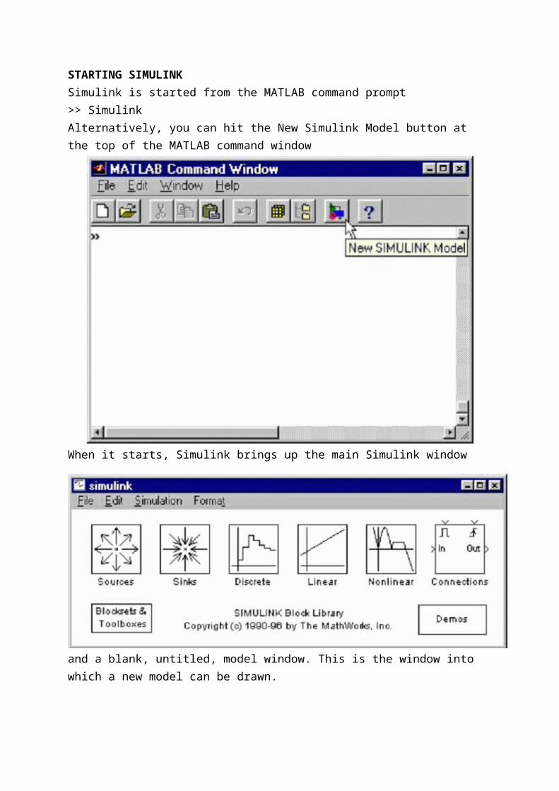
STARTING SIMULINK Simulink is started from the MATLAB command prompt >> Simulink Alternatively, you can hit the New Simulink Model button at the top of the MATLAB command window

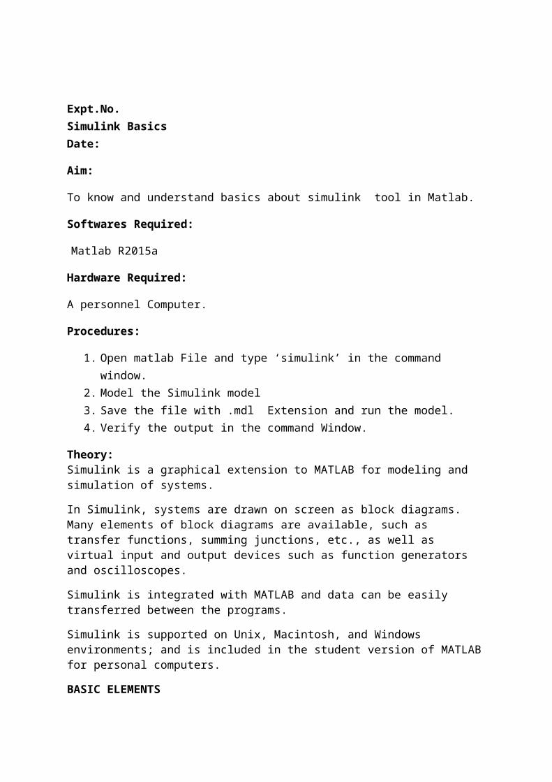
When it starts, Simulink brings up the main Simulink window

and a blank, untitled, model window. This is the window into which a new model can be drawn.

Expt.No. Simulink BasicsDate:

Aim:

To know and understand basics about simulink tool in Matlab.

Softwares Required:

Matlab R2015a

Hardware Required:

A personnel Computer.

Procedures:

1. Open matlab File and type ‘simulink’ in the command window.2. Model the Simulink model3. Save the file with .mdl Extension and run the model.4. Verify the output in the command Window.

Theory:Simulink is a graphical extension to MATLAB for modeling and simulation of systems.

In Simulink, systems are drawn on screen as block diagrams. Many elements of block diagrams are available, such as transfer functions, summing junctions, etc., as well as virtual input and output devices such as function generators and oscilloscopes.

Simulink is integrated with MATLAB and data can be easily transferred between the programs.

Simulink is supported on Unix, Macintosh, and Windows environments; and is included in the student version of MATLAB for personal computers.

BASIC ELEMENTS

There are two major classes of items in Simulink: blocks and lines.

Blocks are used to generate, modify, combine, output, and display signals. Lines are used to transfer signals from one block to another blocks

• Sinks: Used to output or display signals

• Discrete: Linear, discrete-time system elements (transfer functions, state-space models, etc.)

• Linear: Linear, continuous-time system elements and connections (summing junctions, gains, etc.)

RUNNING SIMULATIONS

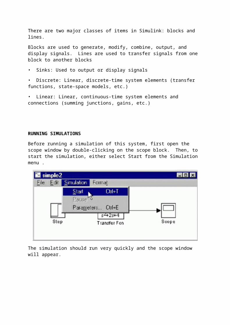
Before running a simulation of this system, first open the scope window by double-clicking on the scope block. Then, to start the simulation, either select Start from the Simulation menu .

The simulation should run very quickly and the scope window will appear.

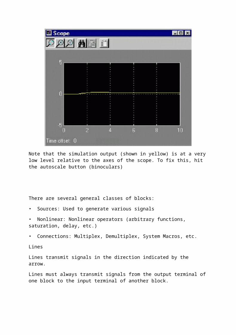
Note that the simulation output (shown in yellow) is at a very low level relative to the axes of the scope. To fix this, hit the autoscale button (binoculars)

There are several general classes of blocks:

• Sources: Used to generate various signals

• Nonlinear: Nonlinear operators (arbitrary functions, saturation, delay, etc.)

• Connections: Multiplex, Demultiplex, System Macros, etc.

Lines

Lines transmit signals in the direction indicated by the arrow.

Lines must always transmit signals from the output terminal of one block to the input terminal of another block.

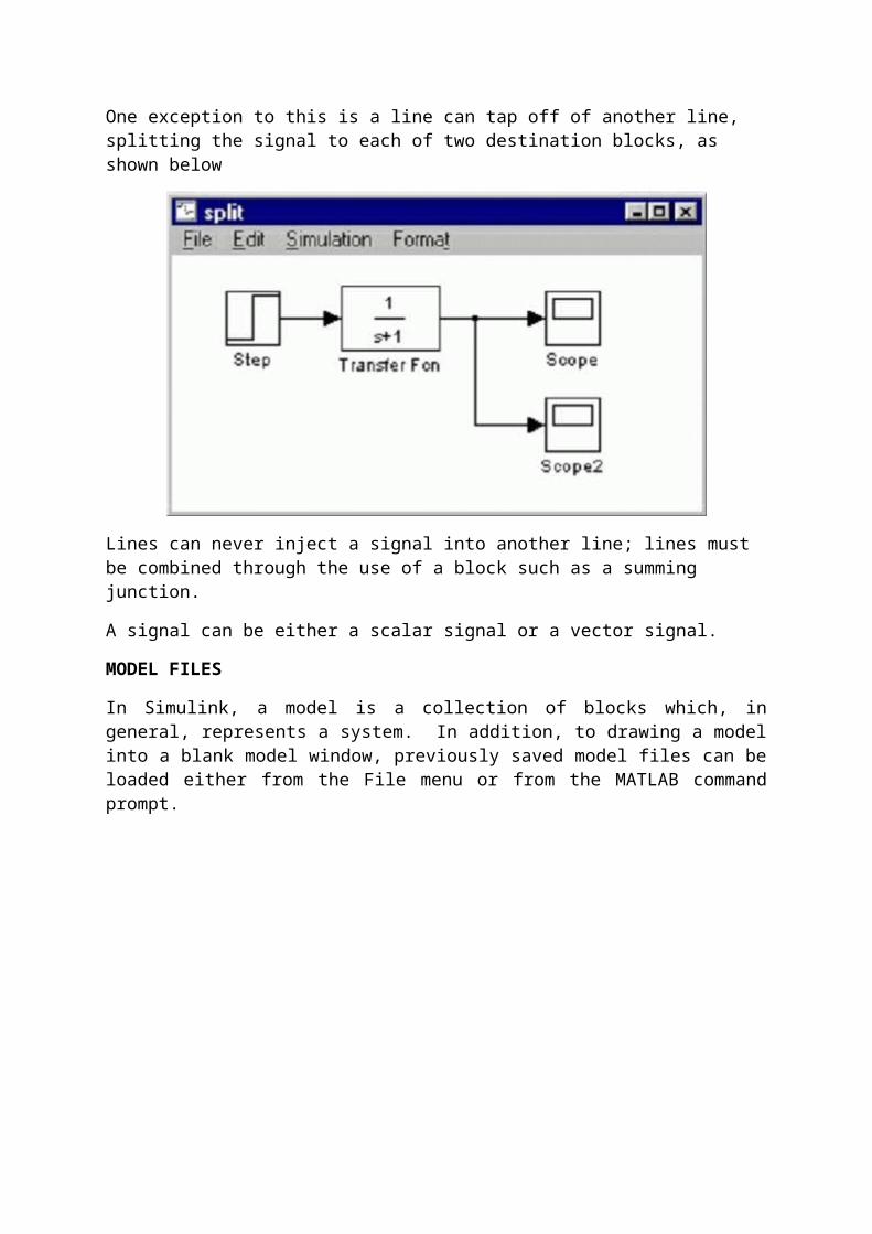
One exception to this is a line can tap off of another line, splitting the signal to each of two destination blocks, as shown below

Lines can never inject a signal into another line; lines must be combined through the use of a block such as a summing junction.

A signal can be either a scalar signal or a vector signal.

MODEL FILES

In Simulink, a model is a collection of blocks which, in general, represents a system. In addition, to drawing a model into a blank model window, previously saved model files can be loaded either from the File menu or from the MATLAB command prompt.

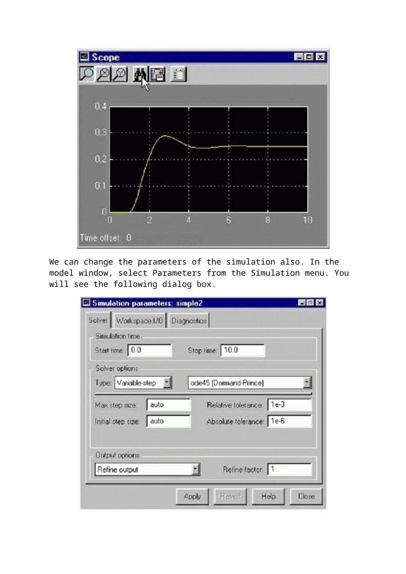
We can change the parameters of the simulation also. In the model window, select Parameters from the Simulation menu. You will see the following dialog box.

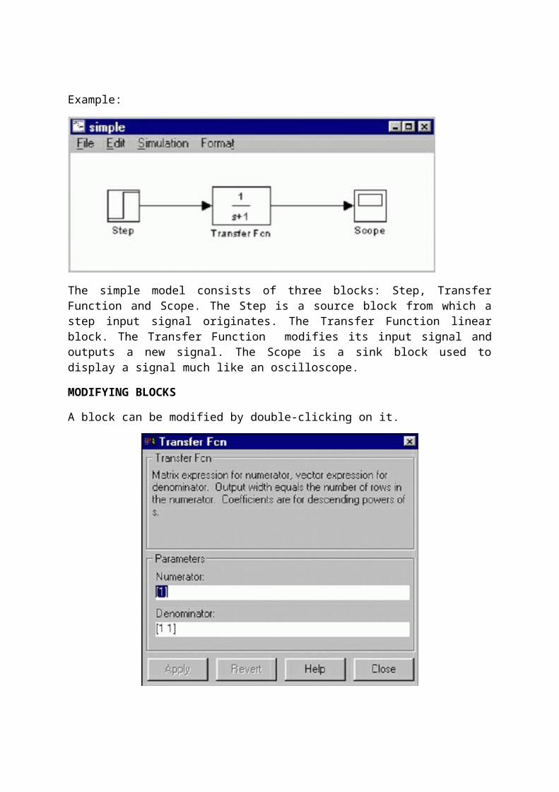
Example:

The simple model consists of three blocks: Step, Transfer Function and Scope. The Step is a source block from which a step input signal originates. The Transfer Function linear block. The Transfer Function modifies its input signal and outputs a new signal. The Scope is a sink block used to display a signal much like an oscilloscope.

MODIFYING BLOCKS

A block can be modified by double-clicking on it.

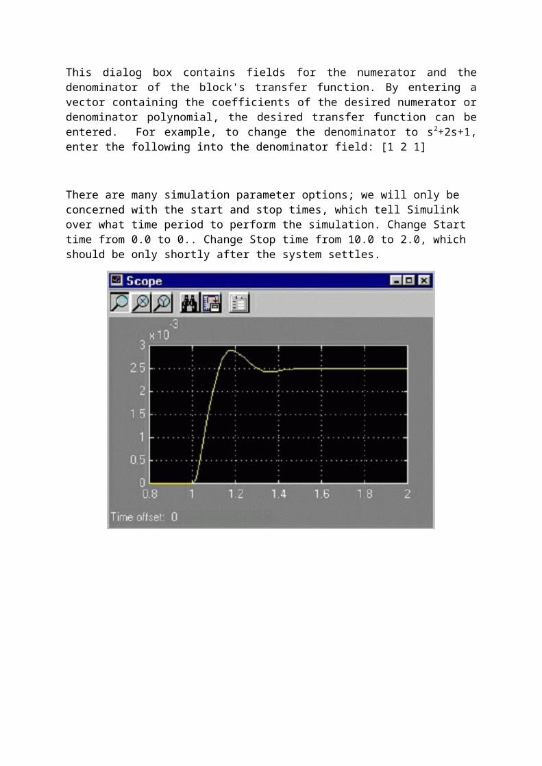
This dialog box contains fields for the numerator and the denominator of the block's transfer function. By entering a vector containing the coefficients of the desired numerator or denominator polynomial, the desired transfer function can be entered. For example, to change the denominator to s2+2s+1, enter the following into the denominator field: [1 2 1]

There are many simulation parameter options; we will only be concerned with the start and stop times, which tell Simulink over what time period to perform the simulation. Change Start time from 0.0 to 0.. Change Stop time from 10.0 to 2.0, which should be only shortly after the system settles.

The "step" block can also be double-clicked, bringing up the following dialog box.

The default parameters in this dialog box generate a step function occurring at time =1 s, from an initial level of zero to a level of 1. The most complicated of these three blocks is the "Scope" block. Double clicking on this brings up a blank oscilloscope screen. When a simulation is performed, the signal which feeds into the scope will be displayed in this window. Use of the autoscale button, which appears as a pair of binoculars.

Result: