SIMULTANEOUS

COMPARISONS AND THE

CONTROL OF TYPE I ERRORS

CHAPTER 6

ERSH 8310 • Lecture 8 • September 18, 2007

Today’s Class

Discussion of the new course schedule.

Take-home midterm (one instead of two) and final.

Simultaneous comparisons.

Schedule, Midterm, and Final Issues

Midterm/Final

Instead of two in-class midterms, we will have one take home midterm.

This frees up four more days of lectures so I can make sure to be more thorough this semester.

Both will be data analysis problems (approximately 2 data sets per test).

Midterm: Handed out 10/11, due 10/23.

Final: Handed out 11/29, due 12/11.

For both the midterm and final you will have no less than a week and a half to complete the task.

You may work in groups on the analysis portion of the test, but your write-up must be your own.

New Tentative Schedule

Date Topic Reading

9/18 Simultaneous Comparisons K6

9/20 Case Studies in ANOVA

9/25 The Linear Model and Its Assumptions K7

9/27 Effect Size, Power, and Sample Size K8

10/2 Introduction to Factorial Designs K10

10/4 The Overall Two-Factor Analysis K11

10/9 Main Effects and Simple Effects K12

10/11 The Analysis of Interaction Components (Midterm handed out, due

10/23 at 11:59:59pm)

K13

10/16 No Class

10/18 No Class

10/23 Midterm discussion

10/25 No Class – Fall Break

10/30, 11/1 The General Linear Model K14

11/6 The Analysis of Covariance K15

11/8 The Single-Factor Within Subjects Design K16

11/13 Further Within Subjects Topics K17

11/15 No Class

11/20 No Class

11/22 No Class – Thanksgiving Break

11/27 The Two-Factor Within-Subject Design K18

11/29 The Mixed Design – Overall Analysis (Final handed out) K19, 20

12/4 No Class – Friday Schedule

12/6 Final Exam Discussion

12/11 Final Exam due at 11:59:59pm

Research Questions and Type I Error

Research Questions and Type I Error

This chapter examines the problem of cumulative Type I

errors and the solutions designed to avoid them.

Researchers are often interested in a set of related

hypothesis (i.e., a family of tests).

The per-comparison error, called α, uses each

comparison as the conceptual unit for determining Type

I error.

The family-wise (FW) Type I error, denoted as αFW,

considers the probability of making one or more Type I

errors in the set of comparisons under scrutiny.

Relationship Between Both Kinds of

Type I Error

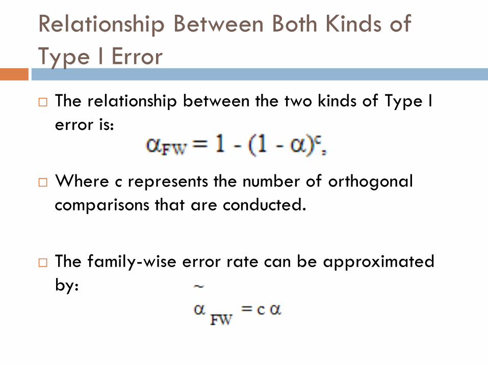
The relationship between the two kinds of Type I

error is:

Where c represents the number of orthogonal

comparisons that are conducted.

The family-wise error rate can be approximated

by:

What Did That Mean???

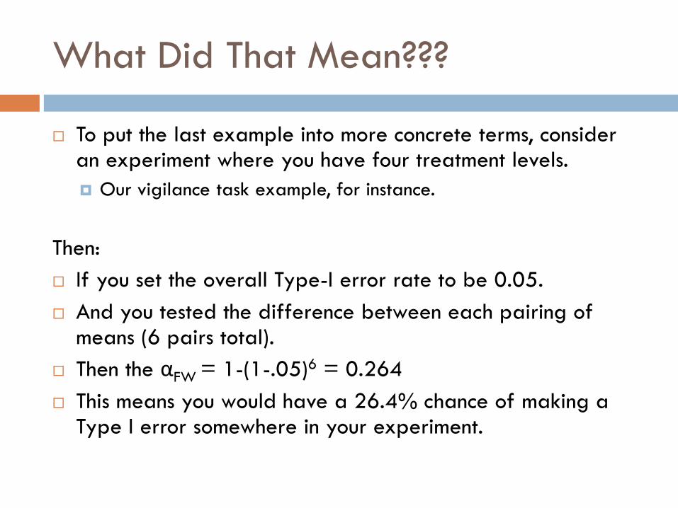
To put the last example into more concrete terms, consider an experiment where you have four treatment levels.

Our vigilance task example, for instance.

Then:

If you set the overall Type-I error rate to be 0.05.

And you tested the difference between each pairing of means (6 pairs total).

Then the αFW = 1-(1-.05)6 = 0.264

This means you would have a 26.4% chance of making a Type I error somewhere in your experiment.

General Plans for Experiments

There are three general plans of an experiments:

1. Testing the primary questions.

e.g., do the treatment means differ generally.

2. Looking at special families of hypotheses.

e.g., contrasts/tests for linear trends/planned comparisons.

3. Exploring the data for unexpected relationships.

e.g., any unplanned tests conducted post-hoc.

Planned Comparisons

Planned Comparisons

Experiments can be designed with specific hypotheses in mind without reference to the outcome of the omnibus F test.

The most widely used strategy to control the family-wise error rate is to evaluate the planned comparisons in a normal way (e.g., α).

The value of orthogonal comparisons lies in the independence of inference.

Meaningful comparisons may contain some nonorthogonalcomparisons.

The nonorthogonal comparisons should be interpreted with particular care.

One may limit the number of planned comparisons (e.g., the number may be dfA = a-1).

Many researchers do limit the number of planned comparisons depending on the research hypotheses and on the complexity of the experiment.

Restricted Sets of Contrasts

Restricted Sets of Contrasts

If you have a plan for the number of contrasts you would like to make a priori, then the following procedures can help adjust your overall Type-I error rate so that you have more protection from error:

Bonferroni

Sidák-Bonferroni

Dunnett’s Test

Any of these tests will help in making decisions when the number of hypothesis tests is known prior to the experiment.

The Bonferroni Procedure

We may apply some corrections to control the overall error rate.

The Bonferroni correction is the most widely applicable family wise control procedure for small families.

Because we may use the Bonferroni test or the Dunn Test that uses:

Where a is the new per comparison significance level and c is the number of comparisons.

Bonferroni Example – SPSS Steps

Under the Post

Hoc…Box

Check Bonferroni

Set your significance

level (Type I error or α)

Bonferroni Example – SPSS Output

This tells us the means are

significantly different for levels

1 and 3, and 1 and 4.

The Sidák-Bonferroni Procedure

This procedure uses:

Which is the exact level (as opposed to the

approximate given in the Bonferroni test).

Dunnett’s Test

It is relevant to all pairwise comparisons involving a

single group.

The Dunnett's test is a specialized family-wise

correction technique that compensates for the

increased number of potential Type I errors that

involves only the control-experimental contrast.

The critical values of t (i.e., tDunnett) are presented in

Appendix A.5 (pp. 582-585).

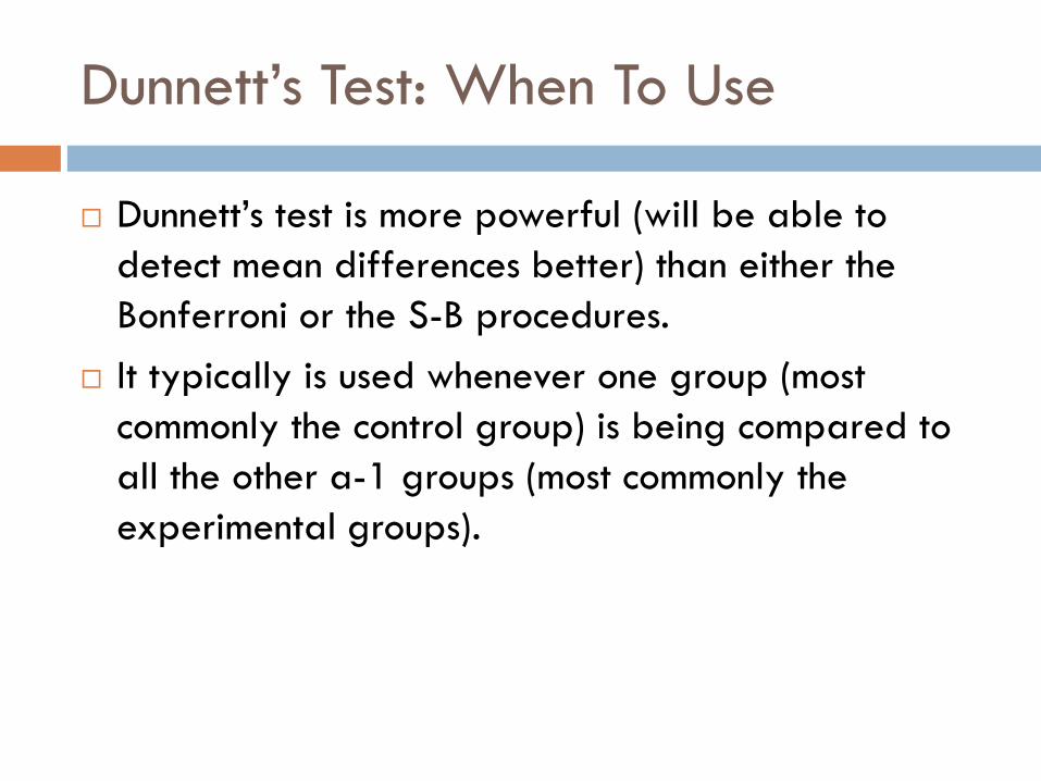
Dunnett’s Test: When To Use

Dunnett’s test is more powerful (will be able to

detect mean differences better) than either the

Bonferroni or the S-B procedures.

It typically is used whenever one group (most

commonly the control group) is being compared to

all the other a-1 groups (most commonly the

experimental groups).

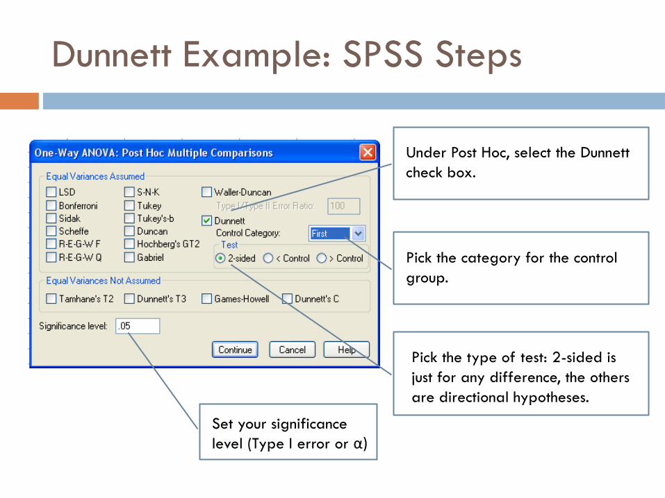
Dunnett Example: SPSS Steps

Under Post Hoc, select the Dunnett

check box.

Pick the category for the control

group.

Pick the type of test: 2-sided is

just for any difference, the others

are directional hypotheses.

Set your significance

level (Type I error or α)

Dunnett Example: SPSS Output

Pairwise Comparisons

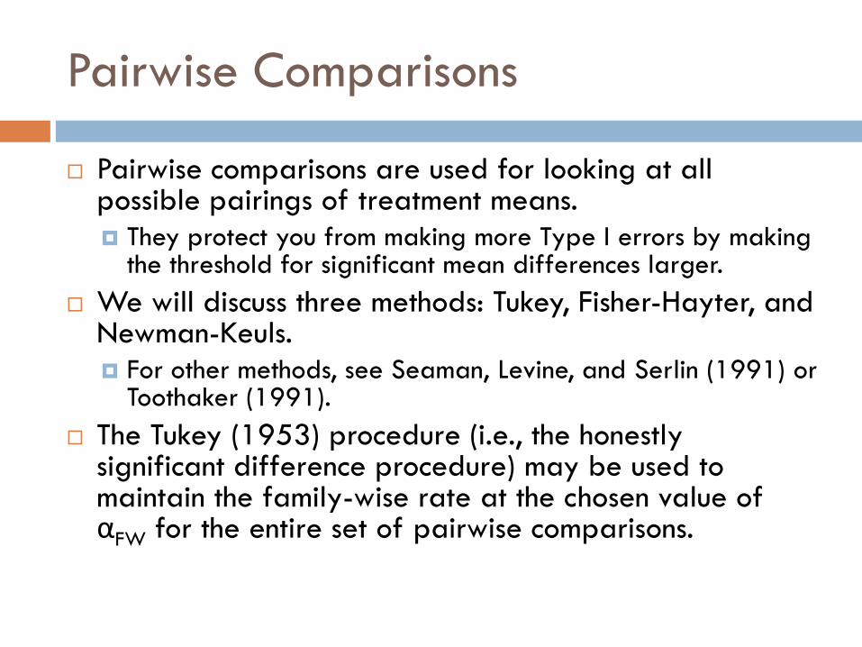
Pairwise Comparisons

Pairwise comparisons are used for looking at all possible pairings of treatment means.

They protect you from making more Type I errors by making the threshold for significant mean differences larger.

We will discuss three methods: Tukey, Fisher-Hayter, and Newman-Keuls.

For other methods, see Seaman, Levine, and Serlin (1991) or Toothaker (1991).

The Tukey (1953) procedure (i.e., the honestly significant difference procedure) may be used to maintain the family-wise rate at the chosen value of αFW for the entire set of pairwise comparisons.

Tukey's HSD Procedure

The pairwise difference between means must exceed

the critical value:

where qa is an entry in Appendix A.6 (see pp. 586-589).

Note the there exists a different critical difference for the

variance heterogeneity case (see Equation 6.8).

Tukey Example: SPSS Steps

Under Post Hoc, select

the Tukey check box.

Set your significance

level (Type I error or α)

Tukey Example: SPSS Output (Part 1)

Tukey Example: SPSS Output (Part 2)

This displays the groups of

means that are not

significantly different from

each other.

Here, 1 and 2 are not

different and 2, 3, and 4

are not different.

The Fisher-Hayter Procedure

Several other procedures have been developed to increase the power of the test.

The Fisher-Hayter procedure uses a sequential approach to testing and involves two steps.

Conduct an omnibus test at aFW level.

If it is significant, then go to the treatment means.

Test all pairwise comparisons using the critical difference:

Note: not in SPSS

The Newman-Keuls and Related

Procedures

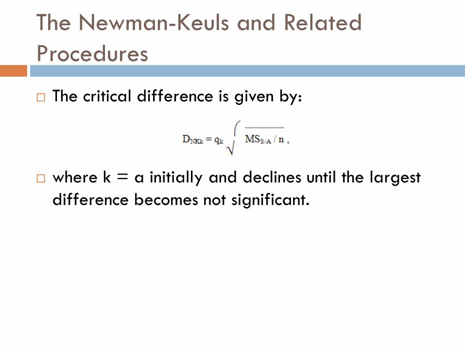
The critical difference is given by:

where k = a initially and declines until the largest

difference becomes not significant.

NK Example: SPSS Steps

Set your significance

level (Type I error or α)

Under Post Hoc, select

the S-N-L check box.

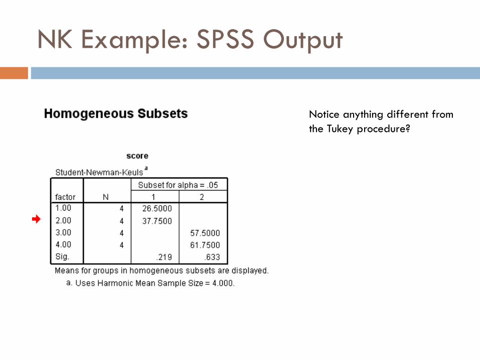
NK Example: SPSS Output

Notice anything different from

the Tukey procedure?

Recommendations from the Book

The process of pairwise comparisons is typically the same, regardless of which test you use.

Look at a bunch of p-values…determine which means are different.

The tests differ in the degree of conservativeness each may present.

The book recommends using either Tukey'sprocedure or the Fisher-Hayter procedure.

Post Hoc Error Correction

Post Hoc Error Correction

Fisher's (1935) procedure (i.e., to test the omnibus F, followed by the unrestricted testing of comparisons among the means, if and only if the overall F is significant), called the least significant difference test, controls the family-wise error indirectly.

This procedure has been criticized by many for not providing adequate control over the family-wise error.

There are several alpha-adjusted techniques.

We will consider the procedure by Scheffé

Scheffé's Procedure

Scheffé's (1953) procedure is a technique that

allows a researcher to maintain the family-wise rate

at a particular value regardless of the number of

comparisons actually conducted.

The critical value is

Where αEW is the experiment wise error rate (see

p. 112).

Scheffé Example: SPSS Steps

Set your significance

level (Type I error or α)

Under Post Hoc, select

the Scheffe check box.

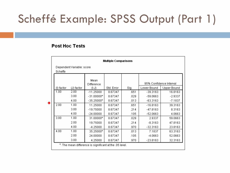
Scheffé Example: SPSS Output (Part 1)

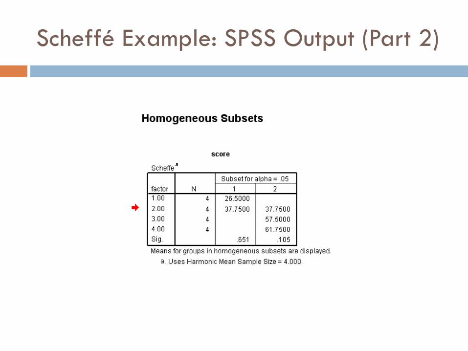
Scheffé Example: SPSS Output (Part 2)

The ANOVA procedure yields an omnibus F test that tells you that at least one group mean is different from the rest.

This class talked about ways in which you could find out which mean that happened to be.

Final Thought

Simultaneous comparisons are specific hypothesis tests that

examine how each mean may differ from all the other means.

By using any of the methods described today, we protect

ourselves from making Type-I errors in our studies.

Next Class

ANOVA Case Study…

An example for the whole class period…

Take a breather from reading and think about what we

are doing overall…big picture.