single and multiple material constraints in thermoelasticity
TRANSCRIPT

Single and multiple material constraints in thermoelasticity
MEHRDAD NEGAHBANDepartment of Engineering Mechanics and The Center for Materials Research and AnalysisW311 Nebraska Hall, University of Nebraska-Lincoln, Lincoln, NE 68588-0526, USA
(Received 28 October 2005� accepted 30 March 2006)
Abstract: Constraints on the possible forms of material response, such as incompressibility or inextensibil-ity, have long been used to simplify constitutive response models, and have resulted in substantial progressin fields such as fluid mechanics and the mechanics of composite materials. A method of imposing theseconstraints for thermoelastic materials is considered that follows steps that remove the need for assumingan additive term resulting from the constraint. In the process, three methods are considered for the separa-tion of the constitutively prescribed part of the response from the part that is in reaction to the constraints.Both the case of single and multiple constraints are considered with extensive examples including specialconsiderations for including effects associated with isotropic or anisotropic thermal expansion.
Key Words: Thermoelastic, material constraint, internal constraint, geometric constraint, multiple constraints, thermo-dynamics, nonlinear elasticity, incompressibility, inextensibility, Bell constraint, isotropic constraints, anisotropic thermalexpansion
1. INTRODUCTION
The theory of material response in the presence of constraints has been looked at by manyauthors and has an important place in the development of material response models. Internalconstraints may take many different forms and may be applied in many different situations.Possibly, the most commonly used and studied material constraints are the geometric con-straints of incompressibility and inextensibility. These and other constraints are idealizationsrepresenting the difficulty to initiate certain events relative to others. For example, the rel-ative rigidity of the fiber compared to the matrix in a fiber reinforced composite can bemodeled by assuming the matrix is inextensible along the fiber directions, such as is doneby Spencer [1]. Another application of material constraints is in the development of theoriesfor problems that are characterized by specific global geometric characteristics of the de-formed body, as was done, for example, in the development of the theory of rods and shellsby Antman and Marlow [2]. The consideration of constraints is not limited to geometricconstraints, as the constraint is simply an imposed relation between the variables of a theory.For example, in Negahban [3] the influence of the yield function in plasticity is introducedas a material constraint.
Mathematics and Mechanics of Solids 11: 000–000, 2006 DOI: 10.1177/1081286506067092
��2006 SAGE Publications
Mathematics and Mechanics of Solids OnlineFirst, published on May 19, 2006 as doi:10.1177/1081286506067092
Copyright 2006 by SAGE Publications.

2 M. NEGAHBAN
The effect of each constraint is normally twofold. A kinematical constraint results ina reduction in the number of degrees of freedom associated with the deformation and, also,simultaneously results in the introduction of the possibility of having certain changes in stresswithout any change in the deformation. For example, irrespective of loading, the lengthof material line elements along a direction of inextensibility do not change. As such, theconstraint has reduced the degrees of freedom associated with the deformation (i.e., certainchanges in the shape of the material cannot occur). In addition, it is obvious that loadsimposed on a material element along a direction of inextensibility cannot change the shape,yet alter the traction and, therefore, change the stress. This implies that stress is not only afunction of the deformation, but that additional information is needed to fully evaluate it.
In a mechanical theory, the primary question is how the constraint influences the evalu-ation of stress. That is, given a deformation, what can be said about the stress, what remainsunknown about the stress until additional information is provided, and what additional infor-mation is needed to fully evaluate the stress. If one does not restrict attention to mechanicaltheories and geometric constraints, one must ask what variables are affected by the introduc-tion of the constraint, in addition to how each variable is influenced.
The consideration of internal constraints has followed several paths depending on thestarting point of the construction and the domain of application. For purely mechanical con-straints, such as incompressibility and inextensibility in elasticity, Ericksen and Rivlin [4]used the balance of energy and the method of Lagrange multipliers to obtain the appropri-ate expression for stress. This method was also used by Green and Adkins [6]. Carlsonand Tortorelli [5] use a similar method replacing the method of Lagrange multipliers by ageometrically motivated argument. An alternate line of development taken by many authorsstarts by assuming that the constraint is “workless”, as was done by Truesdell and Noll [7],and others [8, 9, 10, 11, 12]. For thermoelastic materials, most of the traditional develop-ments are based on imposing the second law of thermodynamics in the form of the entropyproduction inequality or the Clausius–Duhem inequality, such as was done by Rivlin [13],Green and Zerna [14], Green et al. [15], Green and Naghdi [16], and Gurtin and Podio-Guidugli [17]. A notable exception is the work of Batra [18] that uses Hamilton’s extendedprinciple to obtain the effects of constraints, and the work of Casey and Krishnaswamy [19]that separate the second law into two parts following a procedure suggested by Rivlin. Inaddition to the above, references to work on constraints in elasticity can be found in therecent work of Martins and Duda [20], Klisch [21], and Podio-Guidugli [22]. A historicaldiscussion of the work done on constraints is presented at the end of this article.
In the following presentation it is shown how one can impose internal material con-straints starting from the Clausius–Duhem inequality, without introducing additional as-sumptions, such as that of assuming, a priori, an additive decomposition of terms into aconstitutively prescribed part and a part due to the constraint. The method is based on di-rectly including parameters associated with the resulting indeterminacies into the consti-tutive models and then using the Clausius–Duhem inequality to obtain the resulting rela-tions. These added parameters may be of scalar or tensor form, yet the indeterminacy inthe constitutive equations resulting from scalar constraints turn out to be of scalar form. Itis shown that there are multiple ways to decompose the response (stress and entropy) intoa part that is fully determined from the deformation and temperature (extra stress and extraentropy), and one that is in reaction to the constraint (reaction stress and reaction entropy).
THERMOELASTICITY WITH CONSTRAINTS 3
Three methods to group terms are considered. Each method makes the two parts normalto each other using a different definition for normality. The results are obtained for bothsingle and multiple material constrains. Examples are presented for each case includingsingle and multiple constrains. The single constraints considered are isothermally incom-pressible, isothermally inextensible, isothermally Bell constrained with anisotropic thermalexpansion, a general isothermal constraint with anisotropic thermal expansion, a generalisothermal isotropic constraint, and the constraint of zero temperature gradient perpendicu-lar to a material surface. The multiple constraints considered are isothermally incompressibleand inextensible, isothermally incompressible and Bell constrained, isothermally inextensi-ble along two directions, and isothermally inextensible along three directions. The Appendixincludes the examples of isothermally constrained trace of the right Cauchy stretch, isother-mally Bell constrained with isotropic thermal expansion, isothermally inextensible and Bellconstrained, and isothermally Bell constrained and inextensible along two directions.
2. NOTATION
As is common in most descriptions of continuum mechanics, “X” will denote the positionof material particles in a reference configuration, “x” will denote the position in the cur-rent configuration, and “F” will denote the deformation gradient described by dx � FdX.The temperature will be denoted by “� ,” its gradient with respect to changes in the currentconfiguration will be denoted by “g” and its gradient with respect to changes in the refer-ence configuration will be denoted by “G” so that one has d� � g � dx � G � dX, where“�” denotes the dot product. The velocity gradient will be denoted by “L” and is defined asL � �FF�1, where the “�” in �F denotes the material time derivative. A superscript “T” is usedto designate the transpose.
Four response functions will be considered in this development. These four are theresponse functions for the specific free-energy, � , specific entropy, �, Cauchy stress, T,and the heat flux vector, q. The term “response” in this development denotes a dependentvariable for which one must provide a constitutive model (function) in terms of the indepen-dent variables of the theory (the distinction between independent and dependent variablesis not necessarily unique, as, for example, sometimes temperature is replaced for entropyas a dependent variable [2,8]). The independent variables in unconstrained thermoelasticityare normally taken to be position in the reference configuration, X, to allow for variation ofmaterial characteristics from point to point in the material body, deformation gradient, F, tocharacterize the geometric distortion of the body, temperature, � , and its variation in spacedescribed by either G or g.
3. UNCONSTRAINED THERMOELASTIC MATERIAL
An unconstrained thermoelastic material will be defined as a material for which the currentresponse at each material point can be modeled by functions of the current values of the

4 M. NEGAHBAN
deformation gradient, temperature, and temperature gradient. This provides a fairly generalstarting point from which one can develop most every possible model. The constitutivefunctions under this assumption can be written as
� � �†�X�F� ��G�� (1)
� � �†�X�F� ��G�� (2)
T � T†�X�F� ��G�� (3)
q � q†�X�F� ��G�� (4)
where in each equation the left-hand side is the response, and the right hand side is theconstitutive function used to model the response, with the superscript “†” used to designatethe response function.
The second law of thermodynamics, written in the form known as the Clausius–Duheminequality (see [2 or 3]), is given as
� �� � tr�TL�� �� �� � 1
�q � g � 0� (5)
where � is density, and “tr” denotes the trace. This inequality, which is the manifestation ofthe assumption that entropy in a body increases at a rate equal to or greater than the entropyadded to the body by heat, is used in this development to eliminate from consideration mate-rial response functions (constitutive models) that can result in response inconsistent with thesecond law of thermodynamics.
The form of the constitutive model for specific free-energy given in (1) results in amaterial time derivative expressed as
�� � F��� : �F� ���� �� � G��� � �G� (6)
where A��� denotes the partial derivative of � with respect to A (for example, A��� ��Ai j�ei �e j for second order tensor A � Ai j �ei �e j given in the fixed orthonormal base �ei ,
where “” is the tensor product, also known as the dyadic product), A : B � tr�AT B� forsecond order tensors A and B (A : B � Ai j Bi j for A � Ai j �ei �e j and B � Bi j �ei �e j fororthonormal base vectors �ei ). Using the relations L � �FF�1 and tr�AB� � AT : B, one canshow that
tr�TL� � tr�T �FF�1� � tr�F�1T �F� � �F�1T�T : �F� (7)
Using this expression for tr�TL�, substitution of �� from (6) into the Clausius–Duhem in-equality (5), and reorganization results in
[�F���� �F�1T�T ] : �F� �[����� �] �� � [G���] � �G� 1
�q � g � 0� (8)

THERMOELASTICITY WITH CONSTRAINTS 5
This inequality should hold for all possible loading processes. Since the material is in no wayconstrained, at each loading point described by � � �F� ��G�, the loading rate described by�� � � �F� ��� �G� can take any arbitrary value independent of the current value of �, and each
component of �� can be selected independent of its other components. Since the terms in thethree square brackets and the last term are each only a function of �, and since the compo-nents of �� can each take any arbitrary values independent of � and the other componentsof ��, then, as a result of the following lemma, one can conclude that the three terms in thesquare brackets must each be equal to zero and the last term must be less-than or equal tozero if the inequality is to be satisfied under all conditions.
Lemma 1. Consider the inequality�i�1�n
�i�1� � � � � m�� i � �n�1�1� � � � � m� � 0� (9)
which must hold for all admissible i and for all � i , where each �i is an arbitrary boundedfunction of the variable set �1� � � � � m�. If the variables i and � i are independent, andeach� i can be selected independent of the other� i , then the inequality can only be satisfiedif
�i�1� � � � � m� � 0 i � 1� � � � � n (10)
and
�n�1�1� � � � � m� � 0� (11)
The proof of the lemma is fairly easy and is included in the Appendix. The key to theuse of this lemma is the establishment of the independence of functions �i�1� � � � � m� fromthe selection of � i , the establishment of the independence of the � i from each other, andthe determination that each� i may be selected arbitrarily.
In the case of the inequality given in (8), the conditions needed to invoke the lemma aresatisfied for each set of loading parameters � that result in nonsingular response functions.As stated above, each term in the square brackets must be equal to zero, and the last term onthe left-hand side of (8) must be less than or equal to zero resulting in the relations
TT � �F���FT � (12)
� � ������ (13)
G��� � 0� (14)
1
�q � g � 0� (15)
The first and second equations in this set relate the Cauchy stress and specific entropy toderivatives of the specific free-energy, the third establishes that the specific free-energy cannever depend on temperature gradient, and the inequality states that the heat flux vector can

6 M. NEGAHBAN
never have a positive projection along the direction of the temperature gradient, yielding thephysical understanding that heat always flows from hot to cold. As can be seen, enforcementof the Clausius–Duhem inequality has removed from consideration all models for whichfree-energy, and hence the Cauchy stress and entropy, depend on temperature gradient, onlyallowing heat flux to depend on this variable. Embedded in the development of these re-sults is the assumption that temperature and density are always strictly positive, and density,through the law of conservation of mass, is given in terms of the density in the referenceconfiguration, �o, by the equation � det�F� � �o, clearly establishing it as a function of �and X.
4. A SINGLE MATERIAL CONSTRAINT
A material constraint is a relation between the thirteen components of the loading � ��F� ��G�. For example, the constraint equation describing incompressibility is
det�F� � constant� (16)
where J � det�F� is the volume ratio relative to the volume in the reference configuration.The constant is unity if the reference configuration is taken to be a configuration that thematerial actually takes, such as the initial configuration.
A general constraint is given by scalar function f of the form f �X�F� ��G� � 0. Foreach material point, f represents a relation between the deformation gradient, temperature,and temperature gradient. This can be written in terms of the loading � � �F� ��G� as
f �X��� � 0� (17)
As shown schematically in Figure 1, the constraint represents a surface in the 13-dimensionalspace of �. Even though one can have several simultaneous constraint conditions, focuswill be first put on a single scalar constraint. If more than one constraint condition exists,they need to be compatible in the sense that satisfying one constraint will not exclude thepossibility of satisfying the others. Such issues will be addressed in the next section.
The existence of a material constraint also changes the characteristics of the constitutiveresponse functions. For example, as mentioned in the introduction, the addition of load alongthe direction of inextensibility will not result in any changes in shape and, therefore, willnot result in changes of the deformation gradient, even though it will increase the traction.The stress, defined in terms of the traction, therefore can change without any change inthe deformation. As a result, the stress is no longer fully determined by the knowledge of�X�F� ��G�. Let p be a scalar1 that provides the additional information needed to calculatethe response (i.e., that information needed, in addition to X and �, to be able to completelyevaluate the response). It will be assumed that all constitutive functions depend on thisadditional variable.2 That is,

THERMOELASTICITY WITH CONSTRAINTS 7
Figure 1. The schematic of the 13-dimensional loading space �, the 12-dimensional surface describedby the constraint f �X��� � 0, an arbitrary loading rate ���, a loading rate �� tangent to the loadingsurface and, therefore, consistent with the constraint, and the normality of the gradient of f to theconstraint surface.
� � �†�X��� p��
T � T†�X��� p��
� � �†�X��� p��
q � q†�X��� p�� (18)
The constraint restricts how the components of � can change. The relation betweenthe rates of change of these components with respect to time can be obtained by taking thematerial time derivative of the constraint to obtain
F� f � : �F� �� f ��� � G� f � � �G � 0� (19)
As can be seen, this is a scalar relation between the thirteen component of �� � � �F� ��� �G�,and thus reduces the degrees of freedom of �� from thirteen to twelve. As a result, one can nolonger arbitrarily assign values to all thirteen components of ��. To simplify the presentationthis equation will be written as
�� f � � �� � 0� (20)
where “�” denotes the general inner product defined by (19). The constraint condition�� f � � �� � 0 states that all admissible loading rates �� are “orthogonal” to �� f �, asshown schematically in Figure 1. That is, the projection of �� onto �� f � is zero. Therefore,from every arbitrary loading rate ��� one can construct an admissible loading rate �� byremoving the portion of ��� that provides a non-zero projection onto �� f �. On the other
8 M. NEGAHBAN
hand, one can construct every arbitrary loading rate ��� by adding to an admissible loadingrate �� an appropriate loading rate along �� f �. The latter can be written as
��� � ��� �� f �� (21)
where is a scalar factor which may be changed as needed. Using this relation, one canconstruct an admissible loading rate �� from any arbitrary loading rate ��� by selecting such that �� � ��� � �� f � satisfies the constraint condition �� f � � �� � 0. This resultsin
�� f � � [ ��� � �� f �] � 0� (22)
and gives as
� �� f � � ����� f � � �� f �
� (23)
Consideration of the case where �� f � � �� f � � 0 is not of any interest since that wouldimply that all the thirteen component of �� f � are zero, excluding the dependence of f on�. It follows that
�� � ��� � �� f � � ����� f � � �� f �
�� f �� (24)
which yields the relations
�F � �F� � �� f � � ����� f � � �� f �
F� f �� (25)
�� � ��� � �� f � � ����� f � � �� f �
� � f �� (26)
�G � �G� � �� f � � ����� f � � �� f �
G� f �� (27)
For the assumed form of the specific free-energy given in (18), the material time deriva-tive is given by3
�� � ���� � ��� p��� �p� (28)
where �� is restricted to loading paths that are consistent with the constraint condition (20).One can write �� in terms of an arbitrary loading rate ��� using (24) to get

THERMOELASTICITY WITH CONSTRAINTS 9
�� � ���� ����� � �� f � � ���
�� f � � �� f ��� f �
�� p��� �p
������� ���� � �� f �
�� f � � �� f ��� f �
�� ��� � p��� �p� (29)
The Clausius–Duhem inequality must hold for admissible � and ��. Let us introduceinto this expression the relation for �� given in (29), and the expressions for �F and �� given in(25) and (26) to get
�
������ ���� � �� f �
�� f � � �� f ��� f �
�� ��� � �p��� �p
� �TT F�T � :
��F� � �� f � � ���
�� f � � �� f �F� f �
�
� ��
���� � �� f � � ���
�� f � � �� f �� � f �
�� 1
�q � g � 0� (30)
Reorganization of the terms yields��
������ ���� � �� f �
�� f � � �� f ��� f �
�� �T
T F�T � : F� f �
�� f � � �� f ��� f �
� ���� f �
�� f � � �� f ��� f �
�� ��� � �TT F�T � : �F�
� �� ��� � �p��� �p � 1
�q � g � 0� (31)
which must hold for every arbitrary ��� � � �F�� ���� �G��, and any arbitrary �p. The readerwill note that the system is linear in ��� and �p, so that one can organize the equation intofive terms, where the first term only contains �F�, the second term only contains ���, the thirdterm only contains �G�, the fourth term only contains �p, and the fifth term is �q � g��� . Inthe reorganized equation, the factor multiplying each rate is a function of X, � and p, andindependent of ��� or �p. Since the conditions of the lemma are satisfied, for the equation tohold for all arbitrary values of ��� and �p, the factors multiplying �F�, ���, �G�, and �p must eachbe zero and the last term on the left-hand side must be less than or equal to zero. The resultof this process is the following five relations:
�F�����F� f �� TT F�T � 0� (32)
��������� f �� �� � 0� (33)
�G�����G� f � � 0� (34)
p��� � 0� (35)

10 M. NEGAHBAN
1
�q � g � 0� (36)
where
� � ������ � �� f �� �TT F�T � : F� f �� ���� f �
�� f � � �� f �� (37)
To simplify the presentation and bring more physical meaning to the terms, from this pointon TE will be used to denote the “extra stress”, and �E will be used to denote the “extraentropy”. These two terms are defined by
TTE � �F���FT � �E � ����� (38)
and are the same expressions for evaluating stress and entropy when there is no constraintpresent. Using these expressions and reorganization of terms will yield the following fiverelations:
TT � TTE ��F� f �FT � (39)
� � �E � �� �� f �� (40)
G��� � ���G� f �� (41)
p��� � 0� (42)
1
�q � g � 0� (43)
which must be augmented by the constraint condition f �X�F� ��G� � 0. The followingconclusions can be drawn from (39)–(43):
1. It directly follows from (42) that free-energy is independent of p.2. The function� is the only term on the right-hand side of (39–41) that may depend on p
since density �, the constraint function f , and free-energy � are all independent of p.As is shown in (37),� can inherit a dependence on p through the Cauchy stress and/orthrough entropy.
3. The dependence of Cauchy stress T and entropy � on p only comes through the scalarfunction� . This follows from the previous comment and Equations (39) and (40).
4. For constraint functions of the form f �X�G� that exclusively restrain the temperaturegradient, it can be shown that� , T and � are all independent of p. The independence of� from p follows from the fact that for this type of constraint F� f � � 0 and �� f � � 0,so that from (37) one can conclude that � only depends on f , � , and �, all three ofwhich are independent of p. The independence of T and � from p then directly followsfrom Equations (39) and (40) since none of the terms on the right-hand side can dependof p.
THERMOELASTICITY WITH CONSTRAINTS 11
5. For cases that � depends on p, it follows from (41) that the constraint equation shouldbe independent of G. In (41) since one knows that � , �, and f are all independent ofp, it follows that G� f � must be zero (i.e., f �X�F� ��).
6. In cases where � depends on p, it follows from the last comment that the free-energy� is independent of temperature gradient G.
7. Either one of the Equations (39)–(41) may be used to evaluate � and, therefore, onecan construct any number of methods to calculate� including, for example,
� ���TT � TT
E�F�T
: F� f �
F� f � : F� f ����TT � TT
E�
:�F� f �FT
�F� f �FT
:�F� f �FT
� ���E � ���� f �
� � f �� � f �� �G��� � G� f �
G� f � � G� f �� (44)
or substitution of (41) into (37) will result in the expression for � given by
� ���TT � TT
E�F�T
: F� f �� ���E � ���� f �
F� f � : F� f �� �� f �� � f �� (45)
Obviously, the use of each expression is contingent on having a nonzero denominator.
The relation of � to the physical constraint comes from the study of the response ofthe material. For example, consider an incompressible material given by the constraint f �det�F�� 1 � 0. For this constraint �f � det�F�F�T : �F so that one has
F� f � � det�F�F�T � F�T � � � f � � G� f � � 0� (46)
The response of such a material is therefore given by
TT � TTE �� I� � � �E � (47)
The first equation states that the expression for Cauchy stress derived without considerationof the constraint (TE) falls short of fully describing the Cauchy stress by a term which is ofthe form of an additive hydrostatic stress� I. This has been physically interpreted as sayingthat for an incompressible material the constraint makes it such that one can add any hydro-static stress onto any state of stress without altering its shape. The second equation statesthat for this material the entropy is fully determined from the free-energy, and is independentof p. The other relations, as stated above, require the free-energy to be independent of pand G, and that �q � g��� � 0. It is common to set p equal to � , removing all ambigu-ity in the role and definition of p. It should be noted that for incompressible materials thevolume cannot change even with temperature. Therefore, this constraint does not even ac-commodate thermal expansion. One can construct an isothermally incompressible materialthat accommodates thermal expansion by making the volume change be fully determined bythe temperature change, the value remaining constant if there is no temperature change. Thiswill be considered in a later section.

12 M. NEGAHBAN
Figure 2. The schematic of the intersection of two constraint surfaces in the 13-dimensional loadingspace �.
5. MULTIPLE MATERIAL CONSTRAINTS
In place of a single constraint, let there be n scalar constraints, each given by a constraintequation of the form
fi�X��� � 0� (48)
where i is an integer between 1 and n. For each constraint an additional scalar variable pi
will be added to the constitutive equations so that
� � �†�X��� p1� � � � � pn�� (49)
T � T†�X��� p1� � � � � pn�� (50)
� � �†�X��� p1� � � � � pn�� (51)
q � q†�X��� p1� � � � � pn�� (52)
The differential form of the constraint equations can be written by setting each �fi � 0 toobtain the equations
�� fi� � �� � 0� (53)
As in the case of a single constraint, one can introduce an arbitrary loading rate ��� whichcan be used to extract an admissible loading rate �� that is compatible with all constraints andis written as
�� � ��� � j�� f j�� (54)

THERMOELASTICITY WITH CONSTRAINTS 13
The n scalar coefficients i are selected such that �� is forced to satisfy all the constraintssimultaneously. Substitution of this into the n constraints �� fi� � �� � 0 results in the nequations
�� fi� � [ ��� � j�� f j�] � 0� (55)
Reorganizing this results in the n equations
�� fi� � �� f j� j � �� fi� � ���� (56)
Letting Ai j � �� fi� � �� f j� and ci � �� fi� � ���, one gets a linear system of n equationsdescribed by the equation
Ai j j � ci � (57)
where Ai j are the components of a real symmetric matrix of coefficients [A]. If [A] isinvertible, one can write
i � A�1i j c j � (58)
The invertibility of the coefficient matrix [A] is the key to the existence of i . If [A] is notinvertible, then there can only be non-trivial solutions if the loading is such that all the c j arezero. In general, there is always the possibility that the constraints are inconsistent, or thatthe constraints “lock” all or part of the loading � so that loading rate �� or part of it is forcedto be zero. If the constraint conditions are totally incompatible, a loading � cannot be foundto satisfy all the constraints simultaneously, and, therefore, further consideration of this setof constraints is impractical. Yet, the locking of part or all of the response might still resultin a material that is of practical interest. Figure 3 shows schematics of some of these possiblecases.
It will be assumed that the constraints are consistent and [A] is invertible so that one canalways calculate the i . Under these conditions one obtains
�� � ��� � i�� fi� � ��� � A�1i j c j�� fi� � ��� � A�1
i j [�� f j� � ���]�� fi�� (59)
The specific rates for F, � , and G can be written as
�F � �F� � A�1i j [�� f j� � ���]F� fi��
�� � ��� � A�1i j [�� f j� � ���]�� fi��
�G � �G� � A�1i j [�� f j� � ���]G� fi�� (60)
The material derivative of the free-energy under this condition is given by
�� � ���� � ��� pi ��� �pi � (61)

14 M. NEGAHBAN
Figure 3. The schematic of some of the possible things that can happen when dealing with more thanone constraint.
which can be reorganized as
�� � ����� [���� � �� fi�]A�1i j �� f j�
� � ��� � pi ��� �pi � (62)
Substitution of this and the above relations for �F and �� into the Clausius–Duhem inequalitywill result in the inequality
������ [���� � �� fi�]A�1
i j �� f j�� � ��� � �pi ��� �pi
� �TT F�T
: �F� � A�1
i j [�� f j� � ���]F� fi��
� ��� ��� � A�1
i j [�� f j� � ���]�� fi��� 1
�q � g � 0� (63)
As can be seen, this equation is linear in ��� and �pi so that one can organize it in the form of14�n terms where the first 13�n terms each only contain one of the 13�n components of��� and �pi and the last term is �q�g��� . The multiplying factor for each of the 13�n rates is
independent of rate, so that the only way for the equation to be true for all ��� and �pi is thatthese multiplying factors each be equal to zero. The result of this process is the followingequations:
�F����� jF� f j�� TT F�T � 0� (64)
������� j�� f j�� �� � 0� (65)
�G����� jG� f j� � 0� (66)
pi ��� � 0� (67)

THERMOELASTICITY WITH CONSTRAINTS 15
1
�q � g � 0� (68)
where
� j � ������ � �� fi�� �TT F�T � : F� fi�� ���� fi�
�A�1
i j (69)
Reorganization of the equations now yields
TT � TTE �� jF� f j�FT � (70)
� � �E � � j
��� f j�� (71)
G��� � �� j
�G� f j�� (72)
pi ��� � 0� (73)
1
�q � g � 0� (74)
As in the case of a single constraint, the third and fourth equations can be taken as a constrainton the form of the free-energy. In particular, free-energy can never depend on any of the pi .Also, if the constraint conditions do not depend on the temperature gradient G, then thefree-energy cannot depend on temperature gradient. The Cauchy stress and entropy partiallyinherit such characteristics from the free-energy through the first two equations, with theexplicit dependence on pi given only in the � i . The last equation restricts the possibledirection of heat flux in relation to the direction of the temperature gradient. These equationsmust still be augmented by the n constraint equations fi�X�F� ��G� � 0.
6. GROUPING OF TERMS
It is common in purely mechanical theories with one internal constraint to decompose theCauchy stress into a reaction stress, TR , due to the constraint, and an extra stress, TE ,that is prescribed constitutively in terms of a function of �X�F�(see [7, 9]).4 This additivedecomposition is written as
T � TE � TR� (75)
The decomposition is not unique, but normally refers to the selection
TTE � �F���FT � TT
R � �F� f �FT � (76)
This form of the decomposition need not necessarily result in a physically meaningful sep-aration of terms. One method of obtaining more physically meaningful terms is to removefrom TE the portion along TR . To do this one can write

16 M. NEGAHBAN
T � �TE � aTR�� �1� a�TR� (77)
with the condition that T : TR � �1� a�TR : TR . This requires that
a � TE : TR
TR : TR� (78)
As can be seen by substitution, the term T�E � TE � aTR , that is the newly defined extrastress, becomes
T�TE � TT
E � aTTR � �F���FT � [�F���FT ] : [F� f �FT ]
[F� f �FT ] : [F� f �FT ]F� f �FT � (79)
and is independent of the indeterminate function p. One can take� � � �1�a�� and definea new reaction stress T�T
R � � �F� f �FT to obtain
T � T�E � T�R� (80)
for which the extra stress T�E has no projection along the reaction stress T�R , so that T�E :T�R � 0. For example, for the case of the incompressible material one obtains
T�E � TE � 1
3tr�TE�I� T�R �
1
3tr�T�I� (81)
As can be seen, for this constraint the extra stress T�E is traceless, so that� � becomes equal tothe average normal Cauchy stress. One may interpret this as stating that one can prescribe aconstitutive equation for all but the trace of the Cauchy stress. Therefore, the indeterminacyintroduced by this constraint is in the value of the average normal Cauchy stress Tave �tr�T��3.
Even though the method described above works very well for purely mechanical the-ories, it is not the only method for grouping terms together. There are many methods forseparating the different terms. Each method is distinguished by the criteria used to accom-plish the separation. Here three different methods of decoupling the terms will be studied.This is done in the context of multiple constraints, the single constraint being a special case.In each method one arrives at an expression for Cauchy stress and entropy of the form
T � T� j�E � T� j�
R � � � �� j�E � �� j�
R � (82)
where j refers to the method used. In each case� i � ��� j�i �� �� j�
i and
T� j�TE � TT
E � ��� j�i F� fi�FT � T� j�T
R � � �� j�i F� fi�FT � (83)
�� j�E � �E � ��� j�
i
��� fi�� �
� j�R � ��
�� j�i
��� fi�� (84)
Each method is distinguished by the criteria used to separate � i into� i � ��� j�i �� �� j�
i .

THERMOELASTICITY WITH CONSTRAINTS 17
Method 1.5 This method removes from ����� its projections along each �� fi� so that theremainder is orthogonal to all �� fi�. In this method one starts from the equations
TT F�T � �F����� iF� fi��
��� � ������� i�� fi��
0 � �G����� iG� fi�� (85)
and separate each� i into two terms� i � ���1�i �� ��1�
i with the condition that
[������ ���1�i �� fi�] � �� f j� � 0� (86)
for every j between 1 and n. This condition forces ����� � ���1�i �� fi� to be orthogonal
to every �� f j�. This system of equations can be solved for the unknown ���1�i to obtain
���1�i � ������ � �� f j�A
�1j i � (87)
Since �, � , fi , and A�1j i are all independent of the indeterminate functions pi , each ���1�
i isindependent of pi and so is the term ������ ���1�
i �� fi�. The determination of � ��1�i can
be done through the relation
����� � �� f j� � �F��� : F� f j�� ������� f j�� �G��� � G� f j�� (88)
After substitution of (85) and elimination of terms this yields
� ��1�i � ��TT F�T � : F� f j�� ���� f j�
A�1
j i � (89)
As can be seen, each � ��1�i contains both the Cauchy stress and entropy, both of which can
depend on the indeterminate pi . Therefore, the indeterminacy in the prescription of theresponse in terms of the loading is concentrated in each � ��1�
i . It is to be noted that thecalculation of ���1�
i and � ��1�i depends on the invertibility of [A], which has already been
assumed in obtaining (85).
Method 2. This method is based on making T�2�TE F�T simultaneously orthogonal to allF� fi�. This is done by starting with the equation
TT F�T � �F����� iF� fi� (90)
and separation of each� i into two terms� i � ���2�i �� ��2�
i with the condition that��F���� ���2�
i F� fi��
: F� f j� � 0� (91)

18 M. NEGAHBAN
for every j . This condition forces �F���� �� iF� fi� to be orthogonal to every F� f j�. Thissystem of equations can be solved for the unknown ���2�
i to obtain
���2�i � � �TT
E F�T
: F� f j�K�1j i (92)
if the inverse of the matrix [K ] with components Ki j � F� fi� : F� f j� exists. Since �,� , fi ,and K�1
j i are all independent of the indeterminate functions pi , each ���2�i is independent of
pi and so is the term �F���� ���2�i F� fi�. The determination of� ��2�
i can be done throughsubstitution back into the first equation to obtain
� ��2�i � �TT F�T
: F� f j�K
�1j i � (93)
As can be seen, each � ��2�i contains the Cauchy stress, which can depend on the indetermi-
nate pi . Unlike the first method, this method is more suited for mechanical constraints. Themethod can still be used in other cases when some of the constraints are non-mechanical.This is done by only solving for the ���2�
i and � ��2�i associated with the mechanical con-
straints.
Method 3. This method is based on making T�3�TE simultaneously orthogonal to all F� fi�FT .This method, as was the case for Method 2, is best suited for mechanical constraints. Theorthogonalization is done by starting from
TT � �F���FT �� iF� fi�FT (94)
and separation of each� i into two terms� i � ���3�i �� ��3�
i with the condition that��F���FT � ���3�
i F� fi�FT�
:�F� f j�FT
� 0� (95)
for every j . This system of equations can be solved for the unknown �� i to obtain
���3�i � �TT
E :�F� f j�FT
K�1
j i (96)
if the inverse of the matrix [K ] with components Ki j � [F� fi�FT ] : [F� f j�FT ] exists. Each���3�
i becomes independent of pi and so is the term �F���� ���3�i F� fi�. The determination
of� ��3�i can be done through substitution back into the first equation to obtain
� ��3�i � TT :
�F� f j�FT
K�1
j i � (97)
As can be seen, each � ��3�i contains the Cauchy stress, which can depend on the indetermi-
nate pi . As for the second method, this method is best suited for mechanical constraints. Themethod can still be used when some of the constraints are non-mechanical. This is done byonly solving for the ���3�
i and� ��3�i associated with the mechanical constraints.

THERMOELASTICITY WITH CONSTRAINTS 19
Figure 4. Reference, current, and the current stress-free configurations of the neighborhood of influenceof a point. The current stress-free configuration is obtained by isothermally unloading the neighborhoodof the point and then rigidly rotating until the deformation gradient U� describing the deformation from o
to � is symmetric.
7. EXAMPLES OF SINGLE CONSTRAINTS
The following are a number of examples of single constraints. Notable among them is thelast example imposing a zero temperature gradient normal to a material surface, which resultsin an indeterminate shear stress on the surface in the direction of the temperature gradient,among other results. Also, among the examples methods are introduced to include isotropicand anisotropic thermal expansion.
Isothermally incompressible: A material that has constant volume at constant tempera-ture is called an isothermally incompressible material. Consider the reference, current, andcurrent stress-free configurations of the neighborhood of a material point as shown in Fig-ure 4, where the current stress-free configuration is obtained by isothermally unloading theneighborhood of influence of each material point and then rigidly rotating it so that the defor-mation gradient U� becomes symmetric. The deformation gradient U� describes the thermalexpansion at the material point, and for the case of isotropic thermal expansion takes the formU� � J ����1�3I if the reference configuration coincides with a real unloaded configurationof the material neighborhood. In general, for anisotropic thermal expansion, U� is a gen-eral symmetric tensor function of the current temperature. The constraint associated withan isothermally incompressible material can be written as det� �F� � 1, and in view of therelation F � �FU�, this can be written as
det�F� � J ����� (98)

20 M. NEGAHBAN
where J ���� � det�U�� is a function of temperature giving the volume ratio associatedwith the unloaded neighborhood at each temperature. An example of this function would beJ ���� � Jo � ��� � �o�, where Jo is the volume ratio at a reference temperature �o, and� is the volumetric coefficient of thermal expansion. The constraint function in this case isf � det�F�� J ���� � 0 with the partial derivatives
F� f � � det�F�F�T � � � f � � �dJ ����d�
� (99)
These partial derivatives result in the following expressions for Cauchy stress and entropy:
T � TE �� det�F�I� � � �E � ��dJ �
d�� (100)
Since the constraint does not depend on G, it is also concluded that specific free-energy isindependent of G. Without any loss of generality, one can define the indeterminate functionp � � det�F� and replace this into the expressions to obtain
T � TE � pI� � � �E � p
�o
dJ �
d�� (101)
where �o is the density at the reference temperature �o, and � det�F� � �o follows fromconservation of mass. The grouping of terms in the three methods presented result in thefollowing expressions:
T�1�TE � TTE �
tr�TTEB�1�� ��E
1
J �dJ �
d�
tr�B�1�� 1
J �2
�dJ �
d�
�2 I�
T�1�TR �tr�TT B�1�� �� 1
J �dJ �
d�
tr�B�1�� 1
J �2
�dJ �
d�
�2 I� (102)
��1�E � �E �tr�TT
E B�1�� ��E
1
J �dJ �
d�
�
�tr�B�1�� 1
J �2
�dJ �
d�
�2� dJ �
d��
��1�R �tr�TT B�1�� �� 1
J�dJ �
d�
�
�tr�B�1�� 1
J �2
�dJ �
d�
�2� dJ �
d�� (103)

THERMOELASTICITY WITH CONSTRAINTS 21
T�2�TE � TTE �
tr�TTE B�1�
tr�B�1�I� T�2�TR � tr�TT B�1�
tr�B�1�I� (104)
��2�E � �E � tr�TTEB�1�
� tr�B�1�
dJ �
d�� ��2�R � tr�TT B�1�
� tr�B�1�
dJ �
d�� (105)
T�3�TE � TTE �
tr�TE�
3I� T�3�TR � tr�T�
3I� (106)
��3�E � �E � tr�TE�
3�
dJ �
d�� ��3�R � tr�T�
3�
dJ �
d�� (107)
Note that J tr�TT B�1� � tr�P�, where P is the second Piola–Kirchhoff stress tensor. Thethird method results in the most physically meaningful separation since Tave � tr�T��3 is theaverage normal stress.
Isothermally inextensible: A material that at constant temperature is inextensible along agiven material direction is called an isothermally inextensible material. Consider a materialin which the material line element along the direction given by the unit vector �ho in thereference configuration at temperature �o has a length dlo and the same line element in thecurrent configuration at temperature � has the length dl � ����dlo and is along the directiongiven by the unit vector �h � F �ho��. Using the relation dl2 � �ho � �C �ho�dl2
o , this constraintcan be written as
�ho � �C �ho� � �2���� (108)
Using the constraint function f � �ho � �C �ho�� �2��� � 0, the partial derivatives are
F� f � � 2� �h �ho� � � f � � �2�d�
d�� (109)
These result in the following expressions for Cauchy stress and entropy:
T � TE � 2��2 �h �h� � � �E � 2�
��
d�
d�� (110)
The grouping of terms in the three methods presented result in the following expressions:
T�1�TE � TTE �
�2
2
�h � �TTE B�1 �h�� 2��E
1�
d�
d�
1��
d�
d�
�2�h �h�
T�1�TR � �2
2
�h � �TT B�1 �h�� 2�� 1�
d�
d�
1��
d�
d�
�2�h �h� (111)

22 M. NEGAHBAN
��1�E � �E � �
2�
�h � �TTE B�1 �h�� 2��E
1�
d�
d�
1��
d�
d�
�2
d�
d��
��1�R � �
2�
�h � �TT B�1 �h�� 2�� 1�
d�
d�
1��
d�
d�
�2
d�
d�� (112)
T�2�TE � TTE �
�2
2�h � �TT
E B�1 �h� �h �h� T�2�TR � �2
2�h � �TT B�1 �h� �h �h� (113)
��2�E � �E � �
2��h � �TT
E B�1 �h�d�d�� ��2�R � �
2��h � �TT B�1 �h�d�
d�� (114)
T�3�TE � TTE � �2 �h � �TT
E�h� �h �h� T�3�TR � �2 �h � �TT �h� �h �h� (115)
��3�E � �E � �2 �h � �TT
E�h�
�
d�
d�� ��3�R � �2 �h � �TT �h�
�
d�
d�� (116)
Obviously the third method results in the most physically meaningful separation since N ��h � �TT �h� is the normal load on the surface perpendicular to the direction of inextensibility,and, therefore, is the normal traction that is made indeterminate by the constraint.
Isothermally Bell constrained with anisotropic thermal expansion: Here an isothermallyBell constrained material will be considered for which tr� �V� � 3, where �V is the left sym-metric factor in the polar decomposition of �F shown in Figure 4. The only difference withthe last example is the fact that the unloaded thermal expansion may be represented by asymmetric U� other than equal triaxial extension. Denoting by �R and �U the orthogonal fac-tor and the right symmetric factor in the polar decomposition of �F, it can be shown that forf � tr� �V�� 3 on has
�f � � �RU��1� : �F� �U��1 �U� :dU�
d���� (117)
so that one will obtain the partial derivatives
F� f � � �RU��1� � � f � � ��U��1 �U� :dU�
d�� (118)
These result in the following expressions for Cauchy stress and entropy:
T � TE �� �V� � � �E � �� �U��1 �U� :
dU�
d�� (119)
The grouping of terms in the three methods presented result in the following expressions:

THERMOELASTICITY WITH CONSTRAINTS 23
T�1�TE � TTE �
tr�TE�V�1�� ��E�U
��1 �U� :dU�
d�
3���U��1 �U� :
dU�
d�
�2�V� (120)
T�1�TR �tr�T �V�1�� �� �U��1 �U� :
dU�
d�
3���U��1 �U� :
dU�
d�
�2�V� (121)
��1�E � �E �tr�TE
�V�1�� ��E�U��1 �U� :
dU�
d�
2�
�3���U��1 �U� :
dU�
d�
�2� �U��1 �U� :
dU�
d�� (122)
��1�R �tr�T �V�1�� �� �U��1 �U� :
dU�
d�
2�
�3���U��1 �U� :
dU�
d�
�2� �U��1 �U� :
dU�
d�� (123)
T�2�TE � TTE �
tr�TE�V�1�
3�V� T�2�TR � tr�T �V�1�
3�V� (124)
��2�E � �E � tr�TE�V�1�
3��U��1 �U� :
dU�
d�� ��2�R � tr�T �V�1�
3��U��1 �U� :
dU�
d�� (125)
T�3�TE � TTE �
tr�TE�V�
tr�B��V� T�3�TR � tr�T �V�
tr�B��V� (126)
��3�E � �E � tr�TE�V�
� tr�B��U��1 �U� :
dU�
d�� ��3�R � tr�T �V�
� tr�B��U��1 �U� :
dU�
d�� (127)
General constraints of the form �f � �F� �� � 0 with anisotropic thermal expansion: Un-der consideration here is a constraint that is naturally described by the deformation gradient�F which is the current deformation gradient evaluated relative to the stress-free configurationfor the current temperature as described in Figure 4. The time rate of change of �f is givenby
��f � �F� �f � : ��F� �� �f ���� (128)
In view of the relation F � �FU�, one has
��F � �FU��1 � FdU��1
dt� (129)
Combining this with the relation6

24 M. NEGAHBAN
dU��1
dt� �U��1 �U�U��1� (130)
and substituting back into ��f results in
��f � [ �F� �f �U��1] : �F���� �f �� [ �FT �F� �f �U��1] :
dU�
d�
���� (131)
It follows that if the constraint is written in the form f �F� ��, as was done in the developmentspresented in the previous sections, the needed partial derivatives are
F� f � � �F� �f �U��1� � � f � � �� �f �� [ �FT �F� �f �U��1] :dU�
d�� G� f � � 0� (132)
Therefore, if the constraint is naturally stated in terms of deformations from the stress-freeconfiguration at the current temperature, for general anisotropic thermal expansion the partialderivatives can be calculated very simply using these expressions. The expression for Cauchystress and entropy will be
TT � TTE �� �F� �f � �FT � � � �E � ��
��� �f �� [ �FT �F� �f �U��1] :
dU�
d�
�� (133)
Isotropic constraints that are invariant to rigid body motions: The type of constraintconsidered here can be written as
f �I1� I2� I3� �� � 0� (134)
where I1 � tr�U�, I2 � tr�U2�, and I3 � tr�U3� are the isotropic invariants of U. The timederivative of the constraint function is given by
�f � f
Ii
�Ii � f
���� (135)
where �I1 � R : �F, �I2 � 2F : �F, �I3 � 3�VF� : �F. Substitution and reorganization yields
�f � [ f
I1R� 2
f
I2F� 3
f
I3VF] : �F� f
���� (136)
Therefore, the two partial derivatives are
F� f � � f
I1R� 2
f
I2F� 3
f
I3VF� � � f � � f
�� (137)
As a result, the expression for Cauchy stress and entropy for a general isotropic constraintthat is invariant to rigid body motions and does not include temperature gradients is

THERMOELASTICITY WITH CONSTRAINTS 25
TT � TTE ��
� f
I1V� 2
f
I2V2 � 3
f
I3V3
�� � � �E � ��
f
�� (138)
A similar expression can be found if the constraint is written as f �I� I I� I I I� �� � 0, whereI � tr�U�, I I � [tr2�U� � tr�U2�]�2, and I I I � det�U� are an alternate set of isotropicinvariants of U. Using the relations �I � R : �F, �I I � [tr�U�R � F] : �F, and �I I I �det�U�F�T : �F, one obtains
TT � TTE ��
�det�V�
f
I I II�
� f
I� tr�V�
f
I I
�V� f
I IV2
�� (139)
This could also be shown using the Cayley–Hamilton theorem. A commonly used alternatemethod is based on the isotropic invariants of C. For example, consider f �I �1 � I �2 � I �3 � �� � 0,where I �1 � tr�C�, I �2 � tr�C2�, and I �3 � tr�C3�. Using �I �1 � 2F : �F, �I �2 � 4�FC� : �F, and�I �3 � 6�FC2� : �F, one obtains
TT � TTE � 2�
� f
I �1B� 2
f
I �2B2 � 3
f
I �3B3
�� (140)
Another method is based on the alternate isotropic invariants of C. For this case f �I �� I I ��I I I �� �� � 0, where I � � tr�C�, I I � � [tr2�C� � tr�C2�]�2, and I I I � � det�C�. Using�I � � 2F : �F, �I I
� � 2[tr�C�F� FC] : �F, and �I I I� � 2det�C��FC�1� : �F, one obtains
TT � TTE � 2�
�det�C�
f
I I I �I�
� f
I �� tr�C�
f
I I �
�B� f
I I �B2
�� (141)
Zero temperature gradient normal to a material surface: The constraint consideredhere is the case where the temperature gradient across a material surface � in the currentconfiguration is zero. For any vector n normal to �, this constraint can be written as
g � n � 0� (142)
Let �o denote the same material surface, but in the reference configuration, and let �e1 and�e2 denote two orthogonal unit vectors on the surface �o so that �e3 � �e1 �e2 is a unit vectorperpendicular to the surface �o. The vectors u1 � F�e1 and u2 � F�e2 are two vectors onthe surface �, and can be used to calculate the normal n to this surface through the relationn � u1 u2 � �F�e1� �F�e1� � det�F��e3F�1, which results after using the relation �Fa� �Fb� � det�F��a b�F�1 for any two vectors a and b. Obviously, such a vector n is notnecessarily a unit vector since n � n � det2�F��e3 � �C�1�e3� need not equal unity. Addingto the expression for n the relation g � GF�1 and substitution into the constraint equationyields the relation
f � G � �C�1�e3� � 0� (143)
where the original constraint has been divided by det�F�. It can be shown that the partialderivatives of this constraint equation become
26 M. NEGAHBAN
F� f � � F�T ��e3 G�G �e3�C�1� � � f � � 0� G� f � � C�1�e3� (144)
Therefore, the expressions for Cauchy stress and entropy can be written as
TT � TTE ��F�T ��e3 G�G �e3�F�1� � � �E � (145)
Using the relations given above, the Cauchy stress can also be expressed as
TT � TTE �
�
det�F��n g� g n�� (146)
Using the third method to decouple the system one obtains
T�3�TE � TTE �
�g � �TTE �n�� �n � �TT
E �g�2
� �n �g� �g �n��
T�3�TR � �g � �TT �n�� �n � �TT �g�2
� �n �g� �g �n�� (147)
where �n � n��n� and �g � g��g� are unit vectors along n and g, respectively. As is obviouslyclear, the term [�g � �TT �n� � �n � �TT �g�]�2 is the shear stress on the surface with normal �nalong the direction �g. An additional result for this constraint is obtained from manipulatingthe condition q � g � 0. Note that given any arbitrary temperature gradient g�, one canconstruct a temperature gradient g � g� � � �n that satisfies the constraint g � �n � 0 byselecting � � g� � �n. Substitution of g into q � g � 0 and reorganization gives
�q� q � �n �n� � g� � 0� (148)
which states that one can change the component of heat flux q along �n by any amountwithout violating the Clausius–Duhem inequality. Similar to the inextensibility constraint,even though not a direct conclusion of this equation, one may interpret this as stating thatif the temperature gradient along a given direction is forced to be zero, then the heat fluxalong that direction will take any value required to satisfy the balance laws and boundaryconditions. In view of (41), it obviously follows that if the constitutive function for thefree-energy is independent of G, this requires that� be zero and results in T � TE .
8. EXAMPLES OF MULTIPLE CONSTRAINTS
In the following examples thermoelastic response in the presence of more than one constraintis considered. In each case the third method of grouping terms will be used to illustrate theresulting forms. For this method T � T�3�E � T�3�R with the property T�3�E : T�3�R � 0 so thatT : T�3�E � T�3�E : T�3�E and T : T�3�R � T�3�R : T�3�R . A number of additional examples related tothe Bell constraint in combination with inextensibility are included in the Appendix.

THERMOELASTICITY WITH CONSTRAINTS 27
Isothermally incompressible and inextensible: A material that is both isothermally incom-pressible and isothermally inextensible along the direction �ho in the reference configurationis described by the two constraints
f1 � det�F�� J ���� � 0� (149)
f2 � �ho � �C �ho�� �2��� � 0� (150)
where J � and � are as described above for single constraints. The associated partial deriva-tives are
F� f1� � det�F�F�T � � � f1� � �dJ �
d�� (151)
F� f2� � 2�F �ho� �ho� � � f2� � �2�d�
d�� (152)
This results in the expressions for Cauchy stress and entropy given as
TT � TTE �� 1 J �I� 2� 2�F �ho� �F �ho�� (153)
� � �E � � 1
�
dJ �
d�� 2� 2
��
d�
d�� (154)
The matrix [K ] with components Ki j � [F� fi�FT ] : [F� f j�FT ] is, therefore, given by
[K ] ��
3J �2 2J ��2
2J ��2 4�4
�� (155)
The inverse of this matrix is given by
[K ]�1 � 1
8J �2�4
�4� �2J ��2
�2J ��2 3J �2
�� (156)
which results in the expressions
T�3�TE � TTE �
1
2
��tr�TE�� �h � �TT
E�h��
I
� 1
2
�tr�TE�� 3 �h � �TT
E�h�� �h �h� (157)
T�3�TR � 1
2
�tr�T�� �h � �TT �h�
�I� 1
2
��tr�T�� 3 �h � �TT �h�
� �h �h� (158)
28 M. NEGAHBAN
��3�E � �E � 1
2�
��tr�TE�� �h � �TT
E�h�� dJ �
d�
� 1
�
�tr�TE�� 3 �h � �TT
E�h���
d�
d�� (159)
��3�R � 1
2�
�tr�T�� �h � �TT �h�
� dJ �
d�� 1
�
��tr�T�� 3 �h � �TT �h�
��
d�
d�� (160)
where �h � F �ho��. As the reader will note, the complexity added by this grouping of termsresults in the orthogonality of T�3�E and T�3�R (i.e., T�3�E : T�3�R � 0).
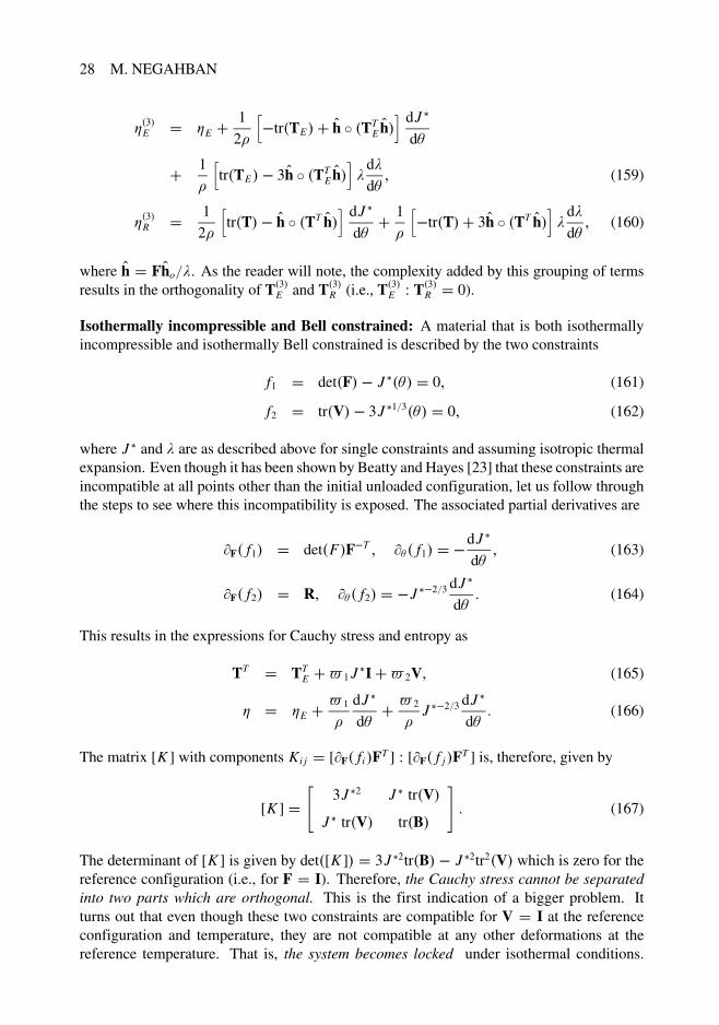
Isothermally incompressible and Bell constrained: A material that is both isothermallyincompressible and isothermally Bell constrained is described by the two constraints
f1 � det�F�� J ���� � 0� (161)
f2 � tr�V�� 3J �1�3��� � 0� (162)
where J � and � are as described above for single constraints and assuming isotropic thermalexpansion. Even though it has been shown by Beatty and Hayes [23] that these constraints areincompatible at all points other than the initial unloaded configuration, let us follow throughthe steps to see where this incompatibility is exposed. The associated partial derivatives are
F� f1� � det�F�F�T � � � f1� � �dJ �
d�� (163)
F� f2� � R� � � f2� � �J ��2�3 dJ �
d�� (164)
This results in the expressions for Cauchy stress and entropy as
TT � TTE �� 1 J �I�� 2V� (165)
� � �E � � 1
�
dJ �
d�� � 2
�J ��2�3 dJ �
d�� (166)
The matrix [K ] with components Ki j � [F� fi�FT ] : [F� f j�FT ] is, therefore, given by
[K ] ��
3J �2 J � tr�V�
J � tr�V� tr�B�
�� (167)
The determinant of [K ] is given by det�[K ]� � 3J �2tr�B�� J �2tr2�V� which is zero for thereference configuration (i.e., for F � I). Therefore, the Cauchy stress cannot be separatedinto two parts which are orthogonal. This is the first indication of a bigger problem. Itturns out that even though these two constraints are compatible for V � I at the referenceconfiguration and temperature, they are not compatible at any other deformations at thereference temperature. That is, the system becomes locked under isothermal conditions.

THERMOELASTICITY WITH CONSTRAINTS 29
Let us return to the original process and recall that the process that was developed requiredthat the matrix [A] with components Ai j � [�� fi�] � [�� f j�] must be invertible. For thesetwo constraints one has
[A] �
�����J �2tr�C�1��
�dJ �
d�
�2
J � tr�V�1�� J ��2�3
�dJ �
d�
�2
J � tr�V�1�� J ��2�3
�dJ �
d�
�2
3� �J ��2�3 dJ�d� �
2
����� � (168)
As can be seen det[A] � 0 for V � I and, therefore, [A] is not invertible at the referenceconfiguration. If [A] cannot be inverted, one cannot find the needed i from (70) to properlydecouple the terms in the Clausius–Duhem inequality and one cannot obtain the results givenin (70)–(74). This is fully consistent with the observation of Beatty and Hayes [23] that theseconstraints are incompatible at all points other than for V � I.
Isothermally inextensible along two directions: A material that is isothermally inextensi-ble along the two directions �ho and �mo in the reference configuration is described by the twoconstraints
f1 � �ho � �C �ho�� �21��� � 0� (169)
f2 � �mo � �C �mo�� �22��� � 0� (170)
where �1 and �2 are the stretches associated with thermal expansions along the respectiveconstraint directions. The associated partial derivatives are
F� f1� � 2�F �ho� �ho� � � f1� � �2�1d�1
d�� (171)
F� f2� � 2�F �mo� �mo� � � f2� � �2�2d�2
d�� (172)
This results in the expressions for Cauchy stress and entropy as
TT � TTE � 2� 1�F �ho� �F �ho�� 2� 2�F �mo� �F �mo�� (173)
� � �E � 2� 1
��1
d�1
d�� 2� 2
��2
d�2
d�� (174)
The matrix [K ] with components Ki j � [F� fi�FT ] : [F� f j�FT ] is, therefore, given by
[K ] ��
4�41 4�2
1�22��h � �m�2
4�21�
22��h � �m�2 4�4
2
�� (175)
where �h � F �ho��1 and �m � F �mo��2. The inverse of this matrix is given by

30 M. NEGAHBAN
[K ]�1 � 1
4�41�
42[1� � �h � �m�4]
��4
2 ��21�
22��h � �m�2
��21�
22��h � �m�2 �4
1
�� (176)
which is clearly singular when the two directions �h and �m are parallel. The expression forstress and entropy can now be written as
T�3�TE � TTE �
�h � �TE�h�� �m � �TE �m�� �h � �m�2
1� � �h � �m�4�h �h
� �m � �TE �m�� �h � �TE�h�� �h � �m�2
1� � �h � �m�4 �m �m� (177)
T�3�TR � �h � �T �h�� �m � �T �m�� �h � �m�21� � �h � �m�4
�h �h
� �m � �T �m�� �h � �T �h�� �h � �m�21� � �h � �m�4 �m �m� (178)
��3�E � �E ��h � �TE
�h�� �m � �TE �m�� �h � �m�2��1
�1� � �h � �m�4
� d�1
d�
� �m � �TE �m�� �h � �TE�h�� �h � �m�2
��2
�1� � �h � �m�4
� d�3
d�� (179)
��3�R � �h � �T �h�� �m � �T �m�� �h � �m�2��1
�1� � �h � �m�4
� d�2
d�
� �m � �T �m�� �h � �T �h�� �h � �m�2��2
�1� � �h � �m�4
� d�3
d�� (180)
Isothermally inextensible along three directions: A material that is isothermally inexten-sible along the three directions �ho, �mo, and �no in the reference configuration is described bythe three constraints
f1 � �ho � �C �ho�� �21��� � 0� (181)
f2 � �mo � �C �mo�� �22��� � 0� (182)
f3 � �no � �C �no�� �23��� � 0� (183)
where �1, �2 and �3 are the stretches associated with thermal expansions along the respectiveconstraint directions. The associated partial derivatives are

THERMOELASTICITY WITH CONSTRAINTS 31
F� f1� � 2�F �ho� �ho� � � f1� � �2�1d�1
d�� (184)
F� f2� � 2�F �mo� �mo� � � f2� � �2�2d�2
d�� (185)
F� f3� � 2�F �no� �no� � � f3� � �2�3d�3
d�� (186)
This results in the expressions for Cauchy stress and entropy as
TT � TTE � 2� 1�F �ho� �F �ho�� 2� 2�F �mo� �F �mo�� 2� 3�F �no� �F �no�� (187)
� � �E � 2� 1
��1
d�1
d�� 2� 2
��2
d�2
d�� 2� 3
��3
d�3
d�� (188)
The matrix [K ] with components Ki j � [F� fi�FT ] : [F� f j�FT ] is, therefore, given by
[K ] � 4
�����4
1 �21�
22��h � �m�2 �2
1�23��h � �n�2
�21�
22��h � �m�2 �4
2 �22�
23� �m � �n�2
�21�
23��h � �n�2 �2
2�23� �m � �n�2 �4
3
���� � (189)
where �h � F �ho��1, �m � F �mo��2 and �n � F �no��3. The inverse of this matrix is given by
[K ]�1 � 1
4D
������� �m��n�4�1
�41
� �h� �m�2�� �h��n�2� �m��n�2�2
1�22
� �h��n�2�� �h� �m�2� �m��n�2�2
1�23
� �h� �m�2�� �h��n�2� �m��n�2�2
1�22
� �h��n�4�1�4
2
� �m��n�2�� �h� �m�2� �h��n�2�2
2�23
� �h��n�2�� �h� �m�2� �m��n�2�2
1�23
� �m��n�2�� �h� �m�2� �h��n�2�2
2�23
� �h� �m�4�1�4
3
������ � (190)
where
D � � �h � �m�4 � � �h � �n�4 � � �m � �n�4 � 2� �h � �m�2� �h � �n�2� �m � �n�2 � 1� (191)
It is clear that [K ] is singular when any two of the three directions �h, �m, and �n are parallel andorthogonal to the third direction. From [K ]�1 one can calculate ���3�
i and� ��3�i as follows:
���3�1 � � 1
2�21 D
� �h � �TE�h� �� �m � �n�4 � 1
� �m � �TE �m��� �h � �m�2 � � �h � �n�2
� �m � �n�2� �n � �TE �n��� �h � �n�2 � � �h � �m�2� �m � �n�2
��� (192)
���3�2 � � 1
2�22 D
� �h � �TE�h��� �h � �m�2 � � �h � �n�2� �m � �n�2
�� �m � �TE �m�
�� �h � �n�4 � 1
�� �n � �TE �n�
�� �m � �n�2 � � �h � �m�2� �h � �n�2
��� (193)

32 M. NEGAHBAN
���3�3 � � 1
2�23 D
� �h � �TE�h��� �h � �n�2 � � �h � �m�2� �m � �n�2
�� �m � �TE �m�
��� �m � �n�2 � � �h � �m�2� �h � �n�2
�� �n � �TE �n�
�� �h � �m�4 � 1
��� (194)
� ��3�1 � 1
2�21 D
� �h � �T �h� �� �m � �n�4 � 1� �m � �T �m�
�� �h � �m�2 � � �h � �n�2
� �m � �n�2� �n � �T �n� �� �h � �n�2 � � �h � �m�2� �m � �n�2��� (195)
� ��3�2 � 1
2�22 D
� �h � �T �h� �� �h � �m�2 � � �h � �n�2� �m � �n�2�� �m � �T �m�
�� �h � �n�4 � 1
�� �n � �T �n�
�� �m � �n�2 � � �h � �m�2� �h � �n�2
��� (196)
� ��3�3 � 1
2�23 D
� �h � �T �h� �� �h � �n�2 � � �h � �m�2� �m � �n�2�� �m � �T �m�
��� �m � �n�2 � � �h � �m�2� �h � �n�2
�� �n � �T �n�
�� �h � �m�4 � 1
��� (197)
The expressions for stress and entropy can now be written as
T�3�TE � TTE � 2�1 ���3�
1�h �h� 2�2 ���3�
3 �m �m� 2�3 ���3�3 �n �n (198)
T�3�TR � 2�1���3�1�h �h� 2�2�
��3�3 �m �m� 2�3�
��3�3 �n �n� (199)
��3�E � �E � 2 ���3�1 �1
�
d�1
d�� 2 ���3�
2 �2
�
d�2
d�� 2 ���3�
3 �3
�
d�3
d�� (200)
��3�R � 2� ��3�1 �1
�
d�1
d�� 2� ��3�
2 �2
�
d�2
d�� 2� ��3�
3 �3
�
d�3
d�� (201)
9. HISTORICAL NOTES
The following comments are a short review of the work on material constraints as relates tothe current development.
Ericksen and Rivlin [4] in 1954 studied large elastic deformations with multiple kinemat-ical constraints. Their development is based on satisfying the balance of energy, assumingthe existence of a stored energy (strain energy) function. In doing so they note that in theabsence of constraints, the balance of energy can be used to fully determine the form of thestress. In the presence of constraints it is shown by the same method used in this article (butapplied to the balance of energy) that the stress is not fully determined by the balance ofenergy. This is due to the fact that all components of the velocity gradient, that both sidesof their equation are multiplied by, can no longer be selected arbitrarily. The result is theintroduction of an indeterminacy in the expression for stress.
THERMOELASTICITY WITH CONSTRAINTS 33
Green and Adkins [6] in 1960 used virtual work as a starting point. This procedureresults in equations identical to the balance of energy. They also point out that the strainenergy function may be regarded as arbitrary up to the addition of a scalar function of theconstraints.
Truesdell and Noll [7] in 1965, seemingly to avoid introduction of internal energy anduse of the balance of energy in the purely mechanical development, replace the above as-sumptions with the assumption that the stress is determined by the deformation gradienthistory only to within a stress that does not do work in any motions satisfying the constraint.As shown by Carlson and Tortorelli [5], in the purely mechanical case for hyperelastic mate-rials this starting assumption of Truesdell and Noll is satisfied when starting from the balanceof energy. Obviously, Truesdell and Noll do not restrict their attention only to hyperelasticmaterials.
Rivlin [13] in 1966 starting from the Clausius–Duhem inequality constructed the formof the stress assuming the existence of multiple kinematical constraints. The procedure pre-sented by Rivlin is similar to that presented in this article, but using the idea of Lagrangemultipliers to remove the constraints on the velocity gradient.
Green et al. [15] in 1970 studied a non-holonomic constraint that is incompatible withthe general thermoelastic constraint presented in this article. The constraint equation theystudied was given as
� i j di j � � i��i � 0�
where di j is the velocity gradient, ��i is the temperature gradient, and � i j and � i are co-efficients that are functions that do not depend on di j and ��i . As a result of this particularselection, constraints such as the isothermally incompressible material constraint presentedhere are not covered by their study. The authors clearly discussed the possibility of the in-clusion of a term of the form � �� , but argue against it for two reasons. First, they excludethis term because this would add an indeterminate term into the entropy. Second, they ex-clude this term “since its physical significance is not clear” to them. These authors providethree methods to obtain the expressions for stress, entropy and heat flux. The first methodthey present is based on assuming an additive decomposition of each term (entropy, stress,and heat flux) into a constitutively prescribed part and a term resulting from the constraint,with the additional assumption that entropy production due to the term resulting from theconstraint is non-negative. The second method is based on eliminating from the Clausius–Duhem inequality the one component of the velocity gradient which is associated with thereduction in the degrees of freedom resulting from the constraint, and then assuming cer-tain resulting coefficients in the Clausius–Duhem inequality are constitutively prescribed.The third method starts with the assumption that each of the four quantities of free-energy,entropy, stress, and heat flux are given by constitutive expressions up to an additive termresulting from the constraint. The last two methods have elements which resemble the pro-cedures presented here.
Gurtin and Podio-Guidugli [17] in 1973 started from an additive decomposition of stress,entropy, and heat flux into constitutively prescribed and reaction induced parts, arrive at theirconclusions introducing a reaction set that is closed under scalar multiplication and assuming
34 M. NEGAHBAN
that the reaction functional is maximal. For the thermodynamic case they show that they canderive the equation that is the starting point of the first method given by Green et al. [15].
Pipkin [24] in 1976 and Rostamian [25] in 1981 have studied internal constraints inlinear elasticity.
Batra [18] in 1987 uses Hamilton’s principle to study and derive the equations for inter-nally constrained elastic materials considering both theories that use temperature and theoriesthat use entropy as their independent variable.
Cohen and Wang [10] in 1987 and Podio-Guidugli and Vianello [26] in 1989 study issuesrelated to material symmetry in constrained elastic materials.
Carlson and Tortorelli [5] in 1996 looked at hyperelastic materials and through geometricarguments arrive from the balance of energy to the expression for the decomposition of stress,without use of the Lagrange multiplier method. Their method does not require that theinternal energy be extended off the constraint manifold.
Casey and Krishnaswamy [19] in 1998 studied internal constraints in thermoelastic ma-terials following a procedure proposed by Rivlin that does not, a priori, assume the existenceof an entropy function. By the a priori assumption that certain constitutive functions do notdepend on temperature gradient, the procedure provides an entropy function based on PartI of the Second Law of Thermodynamics that asserts that the Clausius integral is path in-dependent in strain-temperature space. In addition to discussing the non-uniqueness of theextension of the response functions off the constraint manifold and issues associated withthis, they introduce the “intrinsic” response of the constrained material that results when acurvilinear coordinate is put on the constraint manifold, separating the response into a uniquetangential part to the constraint manifold that describes the constitutively prescribed part anda normal part associated with the reaction to the constraint.
Saccomandi and Beatty [27] in 2002 consider universal relations and solutions for inex-tensible and incompressible isotropic elastic materials, also providing references to relatedwork on universal relations for constrained materials.
10. SUMMARY, COMMENTS AND CONCLUSIONS
The underlying assumption of this article is that the material response must at all times andunder all conditions satisfy the Clausius–Duhem inequality. Using this starting assumption,a procedure is developed to obtain the form of the response of thermoelastic materials in thepresence of single and multiple thermomechanical constraints. The procedure is differentfrom other developments in that the inability of the traditional variables to fully characterizethe response is recognized in the constitutive relations by adding new arguments to make theconstitutive equations complete. The Clausius–Duhem inequality then provides the explicitform of the indeterminate part of the response.
In the second part of this article it is pointed out that the separation of the part of theresponse that is constitutively prescribed from that which is in reaction to the constraint isnot unique and that many different criteria may be used to accomplish this separation. Threemethods for such separation are studied. Each method makes the two parts orthogonal, wherethe definition of orthogonality is different for each method.

THERMOELASTICITY WITH CONSTRAINTS 35
In the third part of this paper examples are presented for both single and multiple con-straints and it is shown how one can introduce isotropic and anisotropic thermal expansioninto constraints that are normally considered only under isothermal conditions. A number ofadditional examples, particularly related to the Bell constraint, are included in the Appendix.
Of the examples, the one on zero temperature gradient normal to a material surface isdifferent from all the others in that it imposes a constraint that includes the temperaturegradient. This constraint introduces an indeterminate shear stress on the surface along thedirection of the temperature gradient. Also, as a result of the constraint, the heat flux normalto the surface is no longer restricted by the Clausius–Duhem inequality and may take anyquantity.
APPENDIX A. PROOF OF LEMMA
The proof of the lemma follows. To prove that �n�1�1� � � � � m� � 0, select all � i � 0.To show that �1�1� � � � � m� � 0, select � i � 0 for i � 2� � � � � n. Now start with the as-sumption that �1�1� � � � � m� �� 0, say, for example, take �1�1� � � � � m� � 0. In this caselet � 1 be a positive number. Since �1�1� � � � � m� and �n�1�1� � � � � m� are bounded andindependent of � 1, and �1�1� � � � � m� � 0, and since � 1 can take any desired value, onecan always increase � 1 until �1�1� � � � � m�� 1 becomes larger than the absolute value of�n�1�1� � � � � m�, so that �1�1� � � � � m�� 1 � �n�1�1� � � � � m� � 0, which results in theviolation of the initial assumption (9). In a similar way, one can show that �1�1� � � � � m�cannot be less than zero, therefore leaving �1�1� � � � � m� � 0 as the only admissible possi-bility.
APPENDIX B. FURTHER EXAMPLES
Isothermally Bell constrained with isotropic thermal expansion: This constraint refersto Bell’s observation that tr�V� � 3 during plastic flow of soft metals, where V is the leftsymmetric factor in the polar decomposition of F � RU � VR. Here an isothermally Bellconstrained material will be considered for which tr� �V� � 3, where �V is the left symmetricfactor in the polar decomposition of �F shown in Figure 4. For the case of isotropic thermalexpansion one can write U� � J ����1�3I, where the reference configuration is selected asany unloaded configuration at reference temperature. In view of F � J �1�3 �F, one can writethis constraint as
tr�V� � 3J �1�3���� (202)
It should be pointed out that volume will not be constant during isothermal loading for a Bellconstrained material as was shown by Beatty and Hayes [23]. For the constraint written asf � tr�V�� 3J �1�3��� � 0, the partial derivatives7 are
F� f � � R� � � f � � �J ��2�3 dJ �
d�� (203)
These result in the following expressions for Cauchy stress and entropy:

36 M. NEGAHBAN
T � TE ��V� � � �E � �� J ��2�3 dJ �
d�� (204)
The grouping of terms in the three methods presented result in the following expressions:
T�1�TE � TTE �
tr�TEV�1�� ��E J ��2�3 dJ �
d�
3��
J ��2�3dJ �
d�
�2 V�
T�1�TR �tr�TV�1�� �� J ��2�3 dJ �
d�
3��
J ��2�3dJ �
d�
�2 V� (205)
��1�E � �E �tr�TE V�1�� ��E J ��2�3 dJ �
d�
�
�3�
�J ��2�3
dJ �
d�
�2� J ��2�3 dJ �
d��
��1�R �tr�TV�1�� �� J ��2�3 dJ �
d�
�
�3�
�J ��2�3
dJ �
d�
�2� J ��2�3 dJ �
d�� (206)
T�2�TE � TTE �
tr�TEV�1�
3V� T�2�TR � tr�TV�1�
3V� (207)
��2�E � �E � tr�TE V�1�
3�J ��2�3 dJ �
d�� ��2�R � tr�TV�1�
3�J ��2�3 dJ �
d�� (208)
T�3�TE � TTE �
tr�TEV�tr�B�
V� T�3�TR � tr�TV�tr�B�
V� (209)
��3�E � �E � tr�TE V�� tr�B�
J ��2�3 dJ �
d�� ��3�R � tr�TV�
� tr�B�J ��2�3 dJ �
d�� (210)
Constraint on tr�C�: The constraint considered here is written as
tr�C� � 3J �2�3���� (211)
where J ���� is the volume ratio representing the unloaded volumetric thermal expansion ofthe material assuming isotropic thermal expansion, with the reference configuration selectedas any unloaded configuration at reference temperature. As for the case of the Bell constraint,the volume is not constant during loading under this constraint. For these conditions, thisconstraint is equivalent to tr� �C� � 3 for �C � �FT �F where �F is as described in Figure 4. Forthe constraint written as f � tr�C�� 3J �2�3��� � 0, the partial derivatives are

THERMOELASTICITY WITH CONSTRAINTS 37
F� f � � 2F� � � f � � �2J ��1�3 dJ �
d�� (212)
These result in the following expressions for Cauchy stress and entropy:
T � TE � 2�B� � � �E � 2�
�J ��1�3 dJ �
d�� (213)
The grouping of terms in the three methods presented result in the following expressions:
T�1�TE � TTE �
tr�TE�� ��E J ��1�3 dJ �
d�
3J �2�3 ��
J ��1�3dJ �
d�
�2 B�
T�1�TR �tr�T�� �� J ��1�3 dJ �
d�
3J �2�3 ��
J ��1�3dJ �
d�
�2 B� (214)
��1�E � �E �tr�TE�� ��E J ��1�3 dJ �
d�
�
�3J �2�3 �
�J ��1�3
dJ �
d�
�2� J ��1�3 dJ �
d��
��1�R �tr�T�� �� J ��1�3 dJ �
d�
�[
�3J �2�3 �
�J ��1�3
dJ �
d�
�2�
]
J ��1�3 dJ �
d�� (215)
T�2�TE � TTE �
tr�TE�
3J �2�3B� T�2�TR � tr�T�
3J �2�3B� (216)
��2�E � �E � tr�TE�
3� J �2�3J ��1�3 dJ �
d�� ��2�R � tr�T�
3� J �2�3J ��1�3 dJ �
d�� (217)
T�3�TE � TTE �
tr�TEB�tr�B2�
B� T�3�TR � tr�TB�tr�B2�
B� (218)
��3�E � �E � tr�TE B�� tr�B2�
J ��1�3 dJ �
d�� ��3�R � tr�TB�
� tr�B2�J ��1�3 dJ �
d�� (219)
Isothermally inextensible and Bell constrained: A material that is both isothermally in-extensible along the direction �ho in the reference configuration and isothermally Bell con-strained is described by the two constraints
f1 � �ho � �C �ho�� �2��� � 0� (220)
f2 � tr�V�� 3J �1�3 � 0� (221)

38 M. NEGAHBAN
where J � and � are as described above for single constraints, and assuming isotropic thermalexpansion associated with the Bell constraint. The associated partial derivatives are
F� f1� � 2�F �ho� �ho� � � f1� � �2�d�
d�� (222)
F� f2� � R� � � f2� � �J ��2�3 dJ �
d�� (223)
This results in the expressions for Cauchy stress and entropy as
TT � TTE � 2� 1�F �ho� �F �ho��� 2V� (224)
� � �E � 2� 1
��
d�
d�� � 2
�J ��2�3 dJ �
d�� (225)
The matrix [K ] with components Ki j � [F� fi�FT ] : [F� f j�FT ] is, therefore, given by
[K ] ��
4�2 2�2 �h � �V �h�2�2 �h � �V �h� tr�B�
�� (226)
The inverse of this matrix is given by
[K ]�1 � 1
4�4�tr�B�� [ �h � �V �h�]2�
�tr�B� �2�2 �h � �V �h�
�2�2 �h � �V �h� 4�2
�� (227)
which results in the expressions
T�3�TE � TTE �
�h � �TE�h� tr�B�� �h � �V �h� tr�TEV�
tr�B�� [ �h � �V �h�]2�h �h
��h � �TE
�h� �h � �V �h�� tr�TEV�
tr�B�� [ �h � �V �h�]2V� (228)
T�3�TR � �h � �T �h� tr�B�� �h � �V �h� tr�TV�
tr�B�� [ �h � �V �h�]2�h �h
� �h � �T �h� �h � �V �h�� tr�TV�
tr�B�� [ �h � �V �h�]2V� (229)
��3�E � �E ��h � �TE
�h� tr�B�� �h � �V �h� tr�TE V�
tr�B�� [ �h � �V �h�]2
�
�
d�
d�
� �h � �TE�h� �h � �V �h�� tr�TEV�
tr�B�� [ �h � �V �h�]2
J ��2�3
�
dJ �
d�� (230)
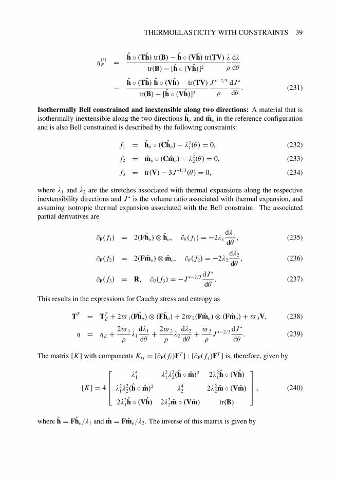
THERMOELASTICITY WITH CONSTRAINTS 39
��3�R � �h � �T �h� tr�B�� �h � �V �h� tr�TV�
tr�B�� [ �h � �V �h�]2
�
�
d�
d�
� �h � �T �h� �h � �V �h�� tr�TV�
tr�B�� [ �h � �V �h�]2
J ��2�3
�
dJ �
d�� (231)
Isothermally Bell constrained and inextensible along two directions: A material that isisothermally inextensible along the two directions �ho and �mo in the reference configurationand is also Bell constrained is described by the following constraints:
f1 � �ho � �C �ho�� �21��� � 0� (232)
f2 � �mo � �C �mo�� �22��� � 0� (233)
f3 � tr�V�� 3J �1�3��� � 0� (234)
where �1 and �2 are the stretches associated with thermal expansions along the respectiveinextensibility directions and J � is the volume ratio associated with thermal expansion, andassuming isotropic thermal expansion associated with the Bell constraint. The associatedpartial derivatives are
F� f1� � 2�F �ho� �ho� � � f1� � �2�1d�1
d�� (235)
F� f2� � 2�F �mo� �mo� � � f2� � �2�2d�2
d�� (236)
F� f3� � R� � � f3� � �J ��2�3 dJ �
d�� (237)
This results in the expressions for Cauchy stress and entropy as
TT � TTE � 2� 1�F �ho� �F �ho�� 2� 2�F �mo� �F �mo��� 3V� (238)
� � �E � 2� 1
��1
d�1
d�� 2� 2
��2
d�2
d�� � 3
�J ��2�3 dJ �
d�� (239)
The matrix [K ] with components Ki j � [F� fi�FT ] : [F� f j�FT ] is, therefore, given by
[K ] � 4
�����4
1 �21�
22��h � �m�2 2�2
1�h � �V �h�
�21�
22��h � �m�2 �4
2 2�22 �m � �V �m�
2�21�h � �V �h� 2�2
2 �m � �V �m� tr�B�
���� � (240)
where �h � F �ho��1 and �m � F �mo��2. The inverse of this matrix is given by

40 M. NEGAHBAN
[K ]�1 � 1
4�41�
42 D
���
��42�tr�B�� [ �m � �V �m�]2�
�21�
22[� �h � �m�2tr�B�� �h � �V �h� �m � �V �m�]
�2�21�
42[� �h � �m�2 �m � �V �m�� �h � �V �h�]
�21�
22[� �h � �m�2tr�B�� �h � �V �h� �m � �V �m�] �2�2
1�42[� �h � �m�2 �m � �V �m�� �h � �V�h�]
��41�tr�B�� [ �h � �V �h�]2� �2�4
1�22[� �h � �m�2 �h � �V �h�� �m � �V �m�]
�2�41�
22[� �h � �m�2 �h � �V�h�� �m � �V �m�] 4�4
1�42[� �h � �m�4 � 1]
��� � (241)
where
D � �[ �h��V �h�]2� [ �m��V �m�]2�2� �h� �m�2 �h��V �h� �m��V �m�� [� �h� �m�4�1]tr�B��� (242)
From [K ]�1 one can calculate ���3�i and� ��3�
i as follows
���3�1 � � 1
2�21 D��h � �TE
�h��[ �m � �V �m�]2 � tr�B��� �m � �TE �m�[� �h � �m�2tr�B�
� �h � �V �h� �m � �V �m�]� tr�TEV�[ �h � �V �h�� � �h � �m�2 �m � �V �m�]�� (243)
���3�2 � � 1
2�22 D��h � �TE
�h�[� �h � �m�2tr�B�� �h � �V �h� �m � �V �m�]� �m � �TE �m�
�[ �h � �V �h�]2 � tr�B���� tr�TE V�[ �m � �V �m�� � �h � �m�2 �h � �V �h�]�� (244)
���3�3 � � 1
D��h � �TE
�h�[ �h � �V �h�� � �h � �m�2 �m � �V �m�]� �m � �TE �m�[ �m � �V �m�
� � �h � �m�2 �h � �V �h�]� tr�TE V�[� �h � �m�4 � 1]�� (245)
The expressions for� ��3�i are similar and can be obtained by removing the “-” sign preceding
each expression and replacing TE with T. The expression for stress can now be written as
T�3�TE � TTE � 2�2
1 ���3�1�h �h� 2�2
2 ���3�3 �m �m� ���3�
3 V (246)
T�3�TR � 2�21�
��3�1�h �h� 2�2
2���3�3 �m �m�� ��3�
3 V� (247)
��3�E � �E � 2 ���3�1 �1
�
d�1
d�� 2 ���3�
2 �2
�
d�2
d�� ���3�
3 J ��2�3
�
dJ �
d�� (248)
��3�R � 2� ��3�1 �1
�
d�1
d�� 2� ��3�
2 �2
�
d�2
d�� �
��3�3 J ��2�3
�
dJ �
d�� (249)
NOTES
1. The selection of p as a scalar is not essential to the development. Without any change in the outcomes,p can be taken as a tensor of any rank. As will be seen later in the development, the imposition ofone scalar valued constraint function results in the introduction of a single scalar function of p in the
THERMOELASTICITY WITH CONSTRAINTS 41
expressions for Cauchy stress and entropy. That is, irrespective of the form of p, its influence is felt bythe response through a single scalar.
2. This assumption is similar to the introduction of a one-parameter family of unconstrained materials, asproposed in [19].
3. For the purposes of this presentation one can assume that �† is a general function of X and �, eventhough as a result of the constraint � can only realize values of �† evaluated at points �X� �� consistentwith the constraint condition f �X� �� � 0. That is, for each material point X, even though�† is definedover the 13-dimensional space of �, � can only take values of �† evaluated over the 12-dimensionalconstraint manifold defined by f �X� �� � 0.If it is desired to assume that �† is only defined over the 12-dimensional constraint manifold, then forthe derivatives to be meaningful as stated one has to extend this function off the constraint manifold.Such extensions are not unique. Any function �†† with the following properties can be used in place of�† in the development to make the derivatives stated meaningful. Take any function �†† defined overthe 13-dimensional space of � with the property that �†† have the same value as �† at every point onthe constraint manifold, and that �†† be differentiable with respect to � at each point on the constraintmanifold. These conditions force ��†† � ��†
at each point on the constraint manifold when restrictingattention to motions on the constraint manifold. Note 5 addresses other issues that might arise with suchnon-unique extensions.
4. The terms “active stress” and “reactive stress” are also used for TE and TR , respectively.5. In reference to the second part of Note 3, the non-uniqueness of the extension of the function for free-
energy off the constraint manifold will not result in a non-uniqueness in the grouping for Method 1, butmight in Method 2 and 3. For Method 1, the method separates ���� into a part that is tangent to theconstraint manifold and a part that is normal to it and then removes the non-unique normal part leavingonly the unique tangential part to be used in the construction of the extra stress and extra entropy. Assuch, Method 1 is similar to the “intrinsic response” introduced by Casey and Krishnaswamy [19].
6. This relation directly follows from taking the derivative of the relation U�U��1 � I.7. The relation F� f � � R can be shown as follows. Since VV�1 � I it follows after taking its derivative
that
dV�1
dt� �V�1 �VV�1� (250)
Since V � V�1B, it follows that
�V � dV�1
dtB�V�1 �B � �V�1 �VV�1B�V�1 �B� (251)
Therefore,
tr� �V� � �tr�V�1 �VV�1B�� tr�V�1 �B�� (252)
Since tr�V�1 �VV�1B� � tr� �V�, it follows that
2tr� �V� � tr�V�1 �B�� (253)
Using B � FFT , taking its time derivative to get �B � �FFT �F �FT and substituting back into the previousexpression yields tr� �V� � tr�RT �F� that can be written as
tr� �V� � R : �F� (254)

42 M. NEGAHBAN
REFERENCES
[1] Spencer, A. J. M. Deformations of Fiber-Reinforced Materials, Clarendon/Oxford University Press, London, 1972.
[2] Antman, S. S. and Marlow, R. S. Material constraints, lagrange multipliers, and compatibility. Applications to rodand shell theories, Archive for Rational Mechanics and Analysis, 116, 257–299 (1991).
[3] Negahban, M. A study of thermodynamic restrictions, constraint conditions, and material symmetry in fully strain-space theories of plasticity, International Journal of Plasticity, 11, 679–724 (1995).
[4] Ericksen, J. L. and Rivlin, R. S. Large elastic deformations of homogeneous anisotropic materials, Journal of Ra-tional Mechanics and Analysis, 3, 281–301 (1954).
[5] Carlson, D. E. and Tortorelli, D. A. On hyperelasticity with internal constraints, Journal of Elasticity, 42, 91–98(1996).
[6] Green, A. E. and Adkins, J. E. Large Elastic Deformations, Clarendon, Oxford, 1960 and 1970.
[7] Truesdell, C. and Noll, W. The Non-Linear Field Theories of Mechanics, Second Edition, Springer, Berlin, 1965/1992.
[8] Wang, C.-C. Mathematical Principles of Mechanics and Electromagnetism, Part A: Analytical and Continuum Me-chanics, Plenum, New York, 1979.
[9] Beatty, M. F. Topics in finite elasticity: Hyperelasticity of rubber, elastomers, and biological tissues-with examples,Applied Mechanics Review, 40, 1699–1734 (1987).
[10] Cohen, H. and Wang, C.-C. On the response and symmetry of elastic materials with internal constraints, Archive forRational Mechanics and Analysis, 99, 1–34 (1987).
[11] Casey, J. A treatment of internally constrained materials, Journal of Applied Mechanics, Transaction of ASME, 62,542–543 (1995).
[12] Casey, J. and Carroll, M. M. A Treatment of internally constrained materials, Journal of Applied Mechanics, Trans-action of ASME, 63, 240 (1996).
[13] Rivlin, R. S. The Fundamental Equations of Nonlinear Continuum Mechanics, Dynamics of Fluids and Plasmas,Academic, New York, 1966.
[14] Green, A. E. and Zerna, W. Theory of Elasticity, Second Edition, Oxford University Press, London, 1968.
[15] Green, A. E., Naghdi, P. M. and Trapp, J. A. Thermodynamics of Continuum with Internal Constraints, InternationalJournal of Engineering Science, 8, 891–908 (1970).
[16] Green, A. E. and Naghdi, P. M. A note on thermodynamics of constrained materials, Journal of Applied Mechanics,Transactions of ASME, 44, 787–789 (1977).
[17] Gurtin, M. E. and Podio-Guidugli, P. The thermodynamics of constrained materials, Archive for Rational Mechanicsand Analysis, 51, 192–208 (1973).
[18] Batra, G. On Hamilton’s principle for thermo-elastic fluids and solids, and internal constraints in thermo-elasticity,Archive for Rational Mechanics and Analysis, 99, 35–59 (1987).
[19] Casey, J. and Krishnaswamy, S. A characterization of internally constrained thermoelastic materials, Mathematicsand Mechanics of Solids, 3, 71–89 (1998).
[20] Martins, L. C. and Duda, F. P. Constrained elastic bodies and universal solutions in the class of plane deformationswith uniform transverse stretch, Mathematics and Mechanics of Solids, 3, 91–106 (1998).
[21] Klisch, S. M. Internally constrained mixtures of elastic continua, Mathematics and Mechanics of Solids, 4, 481–498(1999).
[22] Podio-Guidugli, P. A primer in elasticity, Journal of Elasticity, 58, 1–104 (2000).
[23] Beatty, M. F. and Hayes, M. A. Deformations of an elastic, internally constrained material. Part 1: Homogeneousdeformations, Journal of Elasticity, 29, 1–84 (1992).
[24] Pipkin, A. C. Constraints in linearly elastic materials, Journal of Elasticity, 6, 179–193 (1976).
[25] Rostamian, R. Internal constraints in linear elasticity, Journal of Elasticity, 11, 11–31 (1981).
[26] Podio-Guidugli, P. and Vianello, M. Constraint manifolds for isotropic solids, Archive for Rational Mechanics andAnalysis, 105, 105–121 (1989).
[27] Saccomandi, G. and Beatty, M. F. Universal relations for fiber-reinforced elastic materials, Mathematics and Me-chanics of Solids, 7, 95–110 (2002).