Single Image Super-Resolution Based on Coupled Dictionary and Neural Network Learning

Ke Ma, and Shengchao Liu Department of Computer Sciences University of Wisconsin-Madison {kma, shengchao}@cs.wisc.edu

Abstract

We propose a single image super-resolution method based on coupled dictionaries and neural networks. Our method models the relationship between low- and high-resolution images with a cascade of two distinct learners, and they both contribute to the overall performance, which shares the same ideas with ensemble learning. We discuss how to select the tunable parameters, and compare our method with the baseline method on two datasets. We show that our method is computationally efficient and produces high-quality super-resolution images.

1. Introduction Nowadays, it has become very common that people

use smart phones to take low-resolution pictures, while another interesting trend is that people afford screens of higher and higher resolutions. This creates a gap between low-resolution imaging devices and high-resolution displays. Starting from this point, it is meaningful to come up with an idea to construct high-resolution images from low-resolution ones. Such idea is called image super-resolution (SR), and it has been an active research topic in the computer vision community. It allows better utilization of low-cost image sensors and high-end displays, and is proved to be essential in scientific research such medical and satellite imaging.

While this problem can normally be solved by combining a set of low-resolution images of the same scene aligned with subpixel accuracy, it can be extremely difficult when the number of available input image is small. Although single image super-resolution is generally an ill-posed problem due to insufficient information, various methods can be applied to regularize this problem and produce meaningful results. For example, some people use mathematical models such as curves and patches to model the images as surfaces, and sample the missing locations on the surfaces. Other people use machine learning techniques to learn the relationship between low- and high-resolution images. Our project focuses on recovering the 3x SR version of a given low-resolution image based on machine learning.

[1] proposed a method to reconstruct SR images based on sparse coding. They built a coupled dictionary and optimize for a sparse representation for each patch with respect to some local and global constraints. [2] proposed a method to train a deep convolutional neural network that directly models the mapping from low- to high-resolution images. However, both methods can be computationally expensive. Our project borrows some big ideas from the above methods and adopts a totally different pipeline, which is expected to be efficient and has comparable performance.

2. Related Work Conventional approaches to generating a SR image

require multiple low-resolution images of the same scene. By fusing such low-resolution images, high-resolution images can be reconstructed based on some reasonable assumptions or prior knowledge. But the difficulty is that SR reconstruction can be ill-posed because of insufficient number of images available. Several papers have shown solutions to overcome this difficulty. [3] used a maximum a posteriori framework. [4] proposed an approach using l1 norm minimization and robust regularization. [5] developed a multi-frame image super-resolution approach from a Bayesian view-point.

The second class of SR approaches is based on interpolation. [6] presented the use of B-splines in image enlargement. [7] generalized the Geocuts method, which was proved to have visually appealing results in image SR problem. [8] proposed an approach using a novel generic image prior, with which it could produce state-of-art results. The drawbacks of such methods is the lack of visual complexity of real images.

Another choice is to apply machine learning to solve this problem. [9] used Markov random field solved by belief propagation for reconstruction. [10] extended this approach with Primal Sketch priors, and [11] improved this idea with locally linear embedding. [1] proposed a method based on sparse representation of raw image patches, which represents the state-of-the art, while [2] proposed a method based on deep convolutional network and showed the relationship with sparse representation.

3. Our Method In this section, we introduce how our method works.

We describe the training phase first, and the test phase later. Then we discuss about how to interpret our method from the perspective of ensemble learning.

In order to generate the SR version of an input image, we first decompose the image into square patches of the same size. We call them low-resolution (LR) patches to distinguish them with the high-resolution (HR) patches generated later. Each LR patch is represented as a vector of values between 0 and 1, which is then normalized by subtracting its mean value. The normalized LR patches are fed into the coupled dictionary to generate normalized HR patches. The coupled dictionary is comprised of a low-resolution dictionary and a high-resolution dictionary, and their entries have a one-to-one correspondence. The coupled dictionary models the relationship between normalized LR patches and normalized HR patches, because we are more interested in the textures in the patches rather than their absolute intensities. As the coupled dictionary has limited size, the normalized HR patches generated by it can be regarded as “templates”, which don’t contain intensities and any patch-specific information. To further polish the HR “template” patches, they are concatenated with the original LR patches, and fed into the neural network to produce the final HR patches. As you can expect, the neural network is at lease responsible for two things: to fill in intensities, and to fine tune the HR patches. The HR “template” patches give the neural network a good starting point to magnify the LR patches, without which the task is too underdetermined to have a reasonable solution. The final HR patches are then used to reconstruct the SR version of the image. There is a final step to further improve the quality of the output image, that is, to enforce the global reconstruction constraint. The entire pipeline of our method is shown in Figure 1.

3.1. Training Phase The responsibility of the training phase is to train the

coupled dictionary and the neural network, and record the data for later use. To get the LR and HR patch pairs used

for training, we first downscale the training images to produce the low-resolution counterparts, and then randomly sample LR and HR patches simultaneously. When training the coupled dictionary and the neural network, we use two independent set of training patches, both randomly sampled from the training images. This is because we want the two components to capture different aspects of the relationship between LR and HR, and in practice it accelerates the training of the neural network. Coupled Dictionary Training

The training of the coupled dictionary involves two steps. The first step is to cluster the LR training patches and calculate the centroids of the clusters. These centroids construct the LR dictionary. We use the K-Means clustering algorithm to achieve this. In order to improve the performance, we adopt the K-Means++ algorithm to select initial centroids, and include an online phase after the batch phase to find the global minimum with higher probabilities. The second step is to find the HR counterparts of the LR centroids. We record the indices of the clusters that the LR training patches belong to, and calculate the HR centroids as the average of the HR training patches that belong to the same cluster. These centroids construct the HR dictionary. The coupled dictionary should be overcomplete for better performance. Neural Network Training

The training of the neural network uses the standard Back Propagation algorithm. The architecture of the neural network consists of one input layer, one hidden layer, and one output layer. Because the task considered here can be regarded as regression, we use sigmoid units in the hidden layer and linear units in the output layer.

3.2. Test Phase After the training phase, we need to go through the

entire pipeline to create the SR version of the input images. Here we describe each stage of the pipeline in detail. Patch Extraction

To ensure that the patches cover all the information in the input image, we should decompose the image into patches systematically. Here we extract square patches of the same size column by column, then row by row. To avoid obvious artifacts near the boundaries of the patches, neighboring patches should have some overlap. There are cases when the last patch in a row reaches the right boundary of the image, or the last patch in a column reaches the bottom boundary, so that it is not complete. We handle these cases by mirroring, that is, pretend that there are mirror images about the image boundaries. This technique gives us meaningful boundary patches.

Figure 1. Diagram of the proposed image SR pipeline.

Coupled Dictionary Prediction As stated before, the LR patches are first normalized

and then fed into the coupled dictionary. In the coupled dictionary, we use 1-NN algorithm to find the most similar entry in the LR dictionary. Its index is recorded and used to look up the corresponding entry in the HR dictionary. These HR entries then become the output HR “template” patches. Neural Network Prediction

The HR “template” patches, as well as the LR patches, become the input to the neural network. Combining these two parts is straightforward because patches are stored as vectors internally. The neural network propagates the input values to the output layer via the hidden layer, and generates the output HR patches. Image Reconstruction

The HR patches are then stitched together to reconstruct the HR image, which is exactly the inverse process of the first stage. As in patch extraction, there are patches that fall on the image boundaries. Here we just discard those pixels that are out of bound. We also need to appropriately handle the overlap regions. After the above processing stages, the overlap region from one patch may not be consistent with that from another neighboring patch. We handle this inconsistency by averaging the overlapped pixels. Enforcement of Global Reconstruction Constraint

According to our assumptions, the input LR image should be the blurred and downsampled version of the output HR image. We assume that the blurring filter is a box filter whose size is the same as the scale factor. In our project, the scale factor is 3. Therefore, one pixel in the LR image should correspond to a 3x3 patch in the HR image, and their intensities should satisfy the following equation:

𝐼(#) =𝐼&,(())*

(+,*&+,

3×3

where I(l) is a pixel in the LR image, and I(h)i,j is a pixel in

the corresponding patch in the HR image. Please note that the patch here has totally different meaning from the patches we describe in the above stages. To enforce this global reconstruction constraint, we calculate the difference between the intensity of the pixel and the averaged intensity of the patch, and add this difference to every pixel in the patch. That is:

𝐼&,(()) ← 𝐼&,(

()) + 𝐼 # −𝐼&,()*

(+,*&+,

3×3

Although this looks naïve, it improves the performance in practice.

3.3. Relationship with Ensemble Learning In our SR system, the coupled dictionary and the

neural network are both used for predicting HR patches from LR patches. The training-sets for the coupled dictionary and the neural network are sampled independently, which shares exactly the same idea with Bagging. We hope different learners can capture different aspects of the target function by manipulating their training-sets. The output from the coupled dictionary later becomes part of the input to the neural network, which shares the same idea with Cascading. The coupled dictionary gives the neural network a starting point and reduces its variance, while the neural network further improves the output from the coupled dictionary and reduces its bias. These observations give us a way to understand our system from the perspective of ensemble learning.

4. Experiments and Discussion In this section, we first investigate the two most

important components in our method, that is, the coupled dictionary and the neural network. We perform a set of systematic analyses including plotting learning curves and selecting tunable parameters via cross validation. Then we move our focus to the entire system, analyzing how patch size and overlap width affect the overall performance, and how different components contribute to it. In the end, we apply our method with the selected parameters on two datasets, and compare the results with the baseline method. Please note that when selecting parameters, we consider each parameter alone and ignore the interactions between parameters due to the limited time.

4.1. Analyses of Coupled Dictionary In the following experiments, we consider the

coupled dictionary separately. In the training phase, we sample low-resolution patches and high-resolution patches simultaneously and train a coupled dictionary. In the test phase, we sample low-resolution patches and high-resolution patches, feed low-resolution patches into the coupled dictionary, predict high-resolution patches and compare them with the ground truth. Here, we set the low-resolution patch size to 3x3 and the scale factor to 3, so that the high-resolution patch size is 9x9. We use the measure of mean squared error per patch to evaluate its performance. Dictionary Visualization

We train a coupled dictionary with 10,000 patches and the dictionary size set to 1024. Visualization of the entries in both low-resolution dictionary and high-

resolution dictionary is shown in Figure 2. Black indicates negative values, and white indicates positive values. As expected, entries with the same indices in both dictionaries have good correspondence. Many of the entries show edges in all directions, and the others show relatively smooth gradients; they all represent typical textures or patterns found in the training patches. Effects of Training-set Size

We plot a learning curve for the coupled dictionary with the number of training patches ranging from 2,000 to 50,000. In each iteration, training patches are sampled randomly from images. Each training-set size is repeated for 5 times. Across different settings, we use the same set of 2,000 patches for evaluation to ensure consistency. As shown in Figure 3, increase in the number of training patches leads to improvement of prediction accuracy

when the training-set is relatively small. When the training-set is large, benefits gained from increasing training-set size are overwhelmed by the unbearable computation time. Therefore, we decide that 20,000 training patches should represent a good trade-off between accuracy and efficiency. Effects of Dictionary Size

We also try to vary the size of the coupled dictionary and evaluate its performance. To be specific, we try dictionary sizes of 128, 256, 512, 1024 and 2048. We employ a 6-fold cross validation with 12,000 patches in total to compare different dictionary sizes. The results are shown in Figure 4. When the dictionary is too small, it contains too few useful patch patterns to do the predictions. After the dictionary gets large enough, especially when its size is larger than 512, increasing its size doesn’t improve its performance any longer, only to lengthen its training and test processes. So here we choose the dictionary size to be 512.

Figure 2. Visualization of the entries in the LR dictionary (top) and the HR dictionary (bottom).

Figure 3. Learning curve of the coupled dictionary.

Figure 4. Prediction error for different dictionary sizes.

Alternative Prediction Methods In our initial implementation, we use 1-NN search to

predict high-resolution patches from low-resolution patches. This method is usually called Vector Quantization (VQ) [12], and can be formulated as follows:

𝑎𝑟𝑔𝑚𝑖𝑛𝑪 ||𝒙& − 𝐷𝒄&||=>

&+,

𝑠. 𝑡. ||𝒄&||#B = 1, ||𝒄&||#D = 1, 𝒄& ≥ 0, ∀𝑖 where D is the low-resolution dictionary, and C = [c1, c2, …, cN] is the set of codes for the input low-resolution patches X = [x1, x2, …, xN], which is then used in combination with the high-resolution dictionary to output high-resolution patches. The l0 norm constraint ensures that there is only one non-zero elements in each code, and the l1 norm constraint ensures that its value is 1. There are some alternative methods for this task, which have been proved successful in image classification. One is called Sparse Coding (SC) [12]. The key idea is to relax the constraints, instead of having only one non-zero element in the code, having several ones but are sparse. Hence, a regularization term is needed to ensure the under-determined system has a unique solution:

𝑎𝑟𝑔𝑚𝑖𝑛𝑪 ||𝒙& − 𝐷𝒄&||= + 𝜆||𝒄&||#D>

&+,

Another method is Locality-constrained Linear Coding (LLC) [12], which stresses locality more than sparsity. The key idea is to find a sub-dictionary for each patch, which consists of K entries in the original dictionary that are most similar to the patch, and calculate the code with the sub-dictionary. We remove the shift-invariant constraint in LLC because it is shown not essential. It is now formalized as:

𝑎𝑟𝑔𝑚𝑖𝑛𝑪 ||𝒙& − 𝐷&𝒄&||=>

&+,

where Di is the sub-dictionary for xi. In practice, this is usually more efficient because it doesn’t involve an expensive optimization process.

We do an experiment to test the performance of the coupled dictionary using these three methods. We set the dictionary size to 1024, and employ a 6-fold cross validation with 12,000 patches in total. We empirically set the λ in SC to 0.01, and the K in LLC to 5. The results show that there are significant differences between VQ and LLC (p < 0.01) as well as between LLC and SC (p < 0.001), as in Figure 5. Although SC is the best method in terms of accuracy, it is too expensive in terms of computation, which casts much burden on both the training phase and the test phase. We decide to choose LLC because it improves the accuracy significantly as well, but is no more expensive than VQ.

4.2. Analyses of Neural Network In the following experiments, we consider the neural

network separately. We first train a coupled dictionary with 10,000 patches and the dictionary size set to 1024. We keep the coupled dictionary constant across different settings in the same experiment. In the training phase, we sample low-resolution patches and high-resolution patches simultaneously, feed low-resolution patches into the coupled dictionary to construct the input to the neural network, and then train the neural network. In the test phase, we follow the same procedure to produce the input to the neural network, predict high-resolution patches and compare them with the ground truth. Here, we set the low-resolution patch size to 3x3 and the scale factor to 3, so that the high-resolution patch size is 9x9. We use the measure of mean squared error per patch to evaluate its performance. Overfitting Avoidance

The first thing we want to investigate about the neural network is how to avoid overfitting. Here we adopt the early stopping scheme. We plot a training curve of the neural network with 10,000 training patches and 2,000 validation patches, which is shown in Figure 6. Both the training-set error and the validation-set error decrease rapidly in the first few epochs. The training-set error continues decreasing afterwards, but at a much slower rate. The validation-set error first decreases and then increases. For this specific training process, the validation-set error starts to increase at the 152nd epoch. According to our observations, in most cases this turning point appears before the 500th epoch, so we set the maximum epoch to 500. Empirically we set the validation-set size to be one-fifth of the training-set size.

Figure 5. Prediction error for different prediction methods.

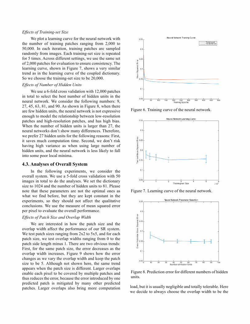
Effects of Training-set Size We plot a learning curve for the neural network with

the number of training patches ranging from 2,000 to 50,000. In each iteration, training patches are sampled randomly from images. Each training-set size is repeated for 5 times. Across different settings, we use the same set of 2,000 patches for evaluation to ensure consistency. The learning curve, shown in Figure 7, shows a very similar trend as in the learning curve of the coupled dictionary. So we choose the training-set size to be 20,000. Effects of Number of Hidden Units

We use a 6-fold cross validation with 12,000 patches in total to select the best number of hidden units in the neural network. We consider the following numbers: 9, 27, 45, 63, 81, and 90. As shown in Figure 8, when there are few hidden units, the neural network is not expressive enough to model the relationship between low-resolution patches and high-resolution patches, and has high bias. When the number of hidden units is larger than 27, the neural networks don’t show many differences. Therefore, we prefer 27 hidden units for the following reasons: First, it saves much computation time. Second, we don’t risk having high variance as when using large number of hidden units, and the neural network is less likely to fall into some poor local minima.

4.3. Analyses of Overall System In the following experiments, we consider the

overall system. We use a 5-fold cross validation with 50 images in total to do the analyses. We set the dictionary size to 1024 and the number of hidden units to 81. Please note that these parameters are not the optimal ones as what we find before, but they are kept constant in the experiments, so they should not affect the qualitative conclusions. We use the measure of mean squared error per pixel to evaluate the overall performance. Effects of Patch Size and Overlap Width

We are interested in how the patch size and the overlap width affect the performance of our SR system. We test patch sizes ranging from 2x2 to 5x5, and for each patch size, we test overlap widths ranging from 0 to the patch side length minus 1. There are two obvious trends: First, for the same patch size, the error decreases as the overlap width increases. Figure 9 shows how the error changes as we vary the overlap width and keep the patch size to be 5. Although not shown here, the same trend appears when the patch size is different. Larger overlaps enable each pixel to be covered by multiple patches and thus reduces the error, because the error introduced by one predicted patch is mitigated by many other predicted patches. Larger overlaps also bring more computation load, but it is usually negligible and totally tolerable. Here

we decide to always choose the overlap width to be the

Figure 6. Training curve of the neural network.

Figure 7. Learning curve of the neural network.

Figure 8. Prediction error for different numbers of hidden units.

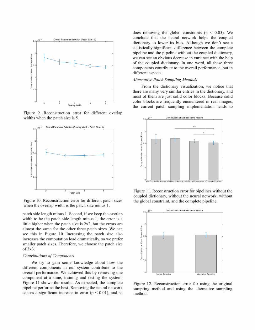
patch side length minus 1. Second, if we keep the overlap width to be the patch side length minus 1, the error is a little higher when the patch size is 2x2, but the errors are almost the same for the other three patch sizes. We can see this in Figure 10. Increasing the patch size also increases the computation load dramatically, so we prefer smaller patch sizes. Therefore, we choose the patch size of 3x3. Contributions of Components

We try to gain some knowledge about how the different components in our system contribute to the overall performance. We achieved this by removing one component at a time, training and testing the system. Figure 11 shows the results. As expected, the complete pipeline performs the best. Removing the neural network causes a significant increase in error (p < 0.01), and so

does removing the global constraints (p < 0.05). We conclude that the neural network helps the coupled dictionary to lower its bias. Although we don’t see a statistically significant difference between the complete pipeline and the pipeline without the coupled dictionary, we can see an obvious decrease in variance with the help of the coupled dictionary. In one word, all these three components contribute to the overall performance, but in different aspects. Alternative Patch Sampling Methods

From the dictionary visualization, we notice that there are many very similar entries in the dictionary, and most of them are just solid color blocks. Because solid color blocks are frequently encountered in real images, the current patch sampling implementation tends to

Figure 9. Reconstruction error for different overlap widths when the patch size is 5.

Figure 10. Reconstruction error for different patch sizes when the overlap width is the patch size minus 1.

Figure 11. Reconstruction error for pipelines without the coupled dictionary, without the neural network, without the global constraint, and the complete pipeline.

Figure 12. Reconstruction error for using the original sampling method and using the alternative sampling method.

sample many of them into the training-set. This actually does harm to the diversity of the dictionary entries. We come up with an alternative patch sampling method, that is, to discard the sampled patches whose variances are lower than a certain threshold. However, our system still needs to know how to handle these solid color blocks. So we decide to use the original sampling method for the neural network.

We do an experiment to verify the effectiveness of this alternative patch sampling method. However, this alternative sampling method fails to show any advantage over the original sampling method, as shown in Figure 12. We choose to stick to out original sampling method.

4.4. Comparison with Baseline Methods Finally, we compare our method with the baseline

methods using the above selected parameters and improvements. The datasets we choose for the comparison include both natural images and artificial ones. Initially, we choose two state-of-the-art methods as our baseline methods: The first method is Bicubic Interpolation (BI), which is widely used in many image processing software. The second method is the Sparse-Coding-based Super-Resolution method (ScSR) [1], which is highly cited and proved to be effective. However, the ScSR code provided by the authors fails to work, so we cannot reproduce their work. Here we only present the comparisons with the former method. Again, we use mean squared error per pixel as our quantitative measure. Flower Dataset

Our first dataset comes from [1] with some modifications, which consists of 50 images of various flowers. 40 images are used for training, and the other for test. All the images are color images, but as our method focuses on grayscale images, they are pre-processed to grayscale when loaded. The images are of various sizes, ranging from around 30,000 pixels to around 150,000 pixels. Most of the images have very delicate textures, which makes the SR process difficult and error-prone.

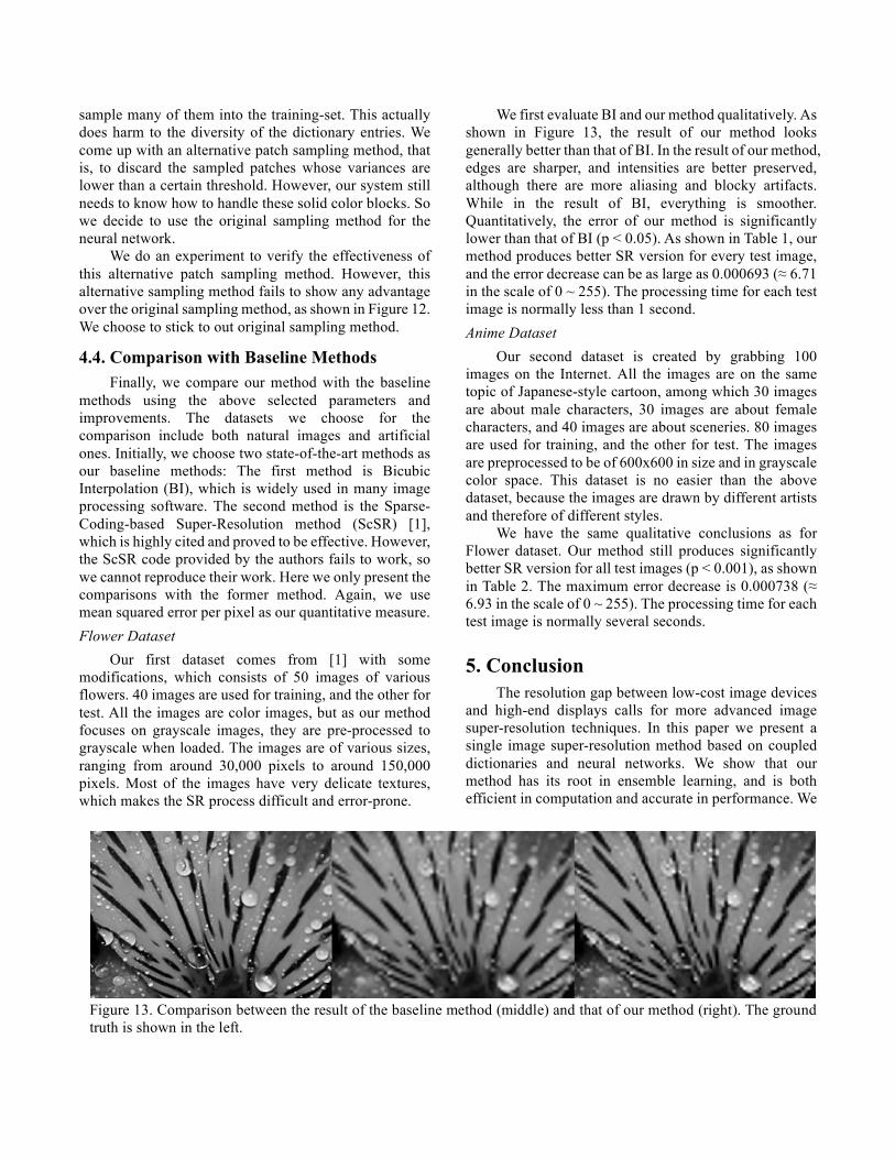
We first evaluate BI and our method qualitatively. As shown in Figure 13, the result of our method looks generally better than that of BI. In the result of our method, edges are sharper, and intensities are better preserved, although there are more aliasing and blocky artifacts. While in the result of BI, everything is smoother. Quantitatively, the error of our method is significantly lower than that of BI (p < 0.05). As shown in Table 1, our method produces better SR version for every test image, and the error decrease can be as large as 0.000693 (≈ 6.71 in the scale of 0 ~ 255). The processing time for each test image is normally less than 1 second. Anime Dataset

Our second dataset is created by grabbing 100 images on the Internet. All the images are on the same topic of Japanese-style cartoon, among which 30 images are about male characters, 30 images are about female characters, and 40 images are about sceneries. 80 images are used for training, and the other for test. The images are preprocessed to be of 600x600 in size and in grayscale color space. This dataset is no easier than the above dataset, because the images are drawn by different artists and therefore of different styles.

We have the same qualitative conclusions as for Flower dataset. Our method still produces significantly better SR version for all test images (p < 0.001), as shown in Table 2. The maximum error decrease is 0.000738 (≈ 6.93 in the scale of 0 ~ 255). The processing time for each test image is normally several seconds.

5. Conclusion The resolution gap between low-cost image devices

and high-end displays calls for more advanced image super-resolution techniques. In this paper we present a single image super-resolution method based on coupled dictionaries and neural networks. We show that our method has its root in ensemble learning, and is both efficient in computation and accurate in performance. We

Figure 13. Comparison between the result of the baseline method (middle) and that of our method (right). The ground truth is shown in the left.

investigate the effects of some tunable parameters in our system, the contributions of different components, and some potential improvements.

If time allows, we would like to investigate how to apply the dictionary optimization algorithm in [12] to our coupled dictionary, so that we can expect a further increase in performance using LLC. Currently the neural network is of simple architecture and uses only sigmoid and linear units, and we would like to try some other activation functions for units and some more complex architectures such as deep network.

Acknowledgement We would like to thank Prof. Mark Craven. His

instructions ultimately led to the creation of this work.

References [1] Yang, J., Wright, J., Huang, T. S., & Ma, Y. (2010). Image super-resolution via sparse representation. Image Processing, IEEE Transactions on, 19(11), 2861-2873. [2] Dong, C., Loy, C. C., He, K., & Tang, X. (2014). Learning a deep convolutional network for image super-resolution. In Computer Vision–ECCV 2014 (pp. 184-199). Springer International Publishing. [3] Hardie, R. C., Barnard, K. J., & Armstrong, E. E. (1997). Joint MAP registration and high-resolution image estimation using a sequence of undersampled images. Image Processing, IEEE Transactions on, 6(12), 1621-1633. [4] Farsiu, S., Robinson, M. D., Elad, M., & Milanfar, P. (2004). Fast and robust multiframe super resolution. Image processing, IEEE Transactions on, 13(10), 1327-1344. [5] Tipping, M. E., & Bishop, C. M. (2006). U.S. Patent No. 7,106,914. Washington, DC: U.S. Patent and Trademark Office. [6] Hou, H. S., & Andrews, H. (1978). Cubic splines for image interpolation and digital filtering. Acoustics,

Speech and Signal Processing, IEEE Transactions on, 26(6), 508-517. [7] Dai, S., Han, M., Xu, W., Wu, Y., & Gong, Y. (2007, June). Soft edge smoothness prior for alpha channel super resolution. In Computer Vision and Pattern Recognition, 2007. CVPR'07. IEEE Conference on (pp. 1-8). IEEE. [8] Sun, J., Sun, J., Xu, Z., & Shum, H. Y. (2008, June). Image super-resolution using gradient profile prior. In Computer Vision and Pattern Recognition, 2008. CVPR 2008. IEEE Conference on (pp. 1-8). IEEE. [9] Freeman, W. T., Pasztor, E. C., & Carmichael, O. T. (2000). Learning low-level vision. International journal of computer vision, 40(1), 25-47. [10] Sun, J., Zheng, N. N., Tao, H., & Shum, H. Y. (2003, June). Image hallucination with primal sketch priors. In Computer Vision and Pattern Recognition, 2003. Proceedings. 2003 IEEE Computer Society Conference on (Vol. 2, pp. II-729). IEEE. [11] Chang, H., Yeung, D. Y., & Xiong, Y. (2004, June). Super-resolution through neighbor embedding. In Computer Vision and Pattern Recognition, 2004. CVPR 2004. Proceedings of the 2004 IEEE Computer Society Conference on (Vol. 1, pp. I-I). IEEE. [12] Wang, J., Yang, J., Yu, K., Lv, F., Huang, T., & Gong, Y. (2010, June). Locality-constrained linear coding for image classification. In Computer Vision and Pattern Recognition (CVPR), 2010 IEEE Conference on (pp. 3360-3367). IEEE.

Table 1. Reconstruction error of BI and our method on the Flower dataset.

Image 1 2 3 4 5 6 7 8 9 10 BI 0.003284 0.000707 0.001514 0.005099 0.000625 0.005014 0.000429 0.000533 0.000381 0.000541

Ours 0.002922 0.000587 0.001307 0.004772 0.000535 0.004320 0.000386 0.000480 0.000324 0.000494

Table 2. Reconstruction error of BI and our method on the Anime dataset.

Image 1 2 3 4 5 6 7 8 9 10 BI 0.002328 0.001872 0.002757 0.005760 0.005992 0.004380 0.003724 0.003821 0.001772 0.001798

Ours 0.002108 0.001588 0.002498 0.005156 0.005254 0.004035 0.003104 0.003456 0.001479 0.001657 Image 11 12 13 14 15 16 17 18 19 20

BI 0.001892 0.002747 0.005891 0.000607 0.005792 0.004160 0.003162 0.001166 0.003057 0.002221 Ours 0.001624 0.002273 0.005508 0.000562 0.005507 0.003898 0.003024 0.001067 0.002859 0.002034