single-image super resolution for multispectral remote sensing data … · 2016-06-10 ·...

SINGLE-IMAGE SUPER RESOLUTION FOR MULTISPECTRAL REMOTE SENSINGDATA USING CONVOLUTIONAL NEURAL NETWORKS

L. Liebel∗, M. Korner

Technical University of Munich, Remote Sensing Technology, Computer Vision Research Group,Arcisstraße 21, 80333 Munich, Germany – {lukas.liebel, marco.koerner}@tum.de

WG ICWG III/VII

KEY WORDS: Single-Image Super Resolution, Deep Learning, Convolutional Neural Networks, Sentinel-2

ABSTRACT:

In optical remote sensing, spatial resolution of images is crucial for numerous applications. Space-borne systems are most likely to beaffected by a lack of spatial resolution, due to their natural disadvantage of a large distance between the sensor and the sensed object.Thus, methods for single-image super resolution are desirable to exceed the limits of the sensor. Apart from assisting visual inspection ofdatasets, post-processing operations—e.g., segmentation or feature extraction—can benefit from detailed and distinguishable structures.In this paper, we show that recently introduced state-of-the-art approaches for single-image super resolution of conventional photographs,making use of deep learning techniques, such as convolutional neural networks (CNN), can successfully be applied to remote sensingdata. With a huge amount of training data available, end-to-end learning is reasonably easy to apply and can achieve results unattainableusing conventional handcrafted algorithms.We trained our CNN on a specifically designed, domain-specific dataset, in order to take into account the special characteristics ofmultispectral remote sensing data. This dataset consists of publicly available SENTINEL-2 images featuring 13 spectral bands, a groundresolution of up to 10 m, and a high radiometric resolution and thus satisfying our requirements in terms of quality and quantity.In experiments, we obtained results superior compared to competing approaches trained on generic image sets, which failed to reasonablyscale satellite images with a high radiometric resolution, as well as conventional interpolation methods.

1. INTRODUCTION

As resolution has always been a key factor for applications usingimage data, methods enhancing the spatial resolution of imagesand thus actively assist in achieving better results are of greatvalue.

In contrast to classical super resolution approaches, using multipleframes of a scene to enhance their spatial resolution, single-imagesuper resolution algorithms have to solely rely on one given inputimage. Even though earth observation missions typically favororbits allowing for acquisition of the same scene on a regular basis,the scenes still change too fast in comparison to the revisit time,e.g., due to shadows, cloud or snow coverage, moving objects or,seasonal changes in vegetation. We hence tackle the problem, asif there was no additional data available.

Interpolation methods, like bicubic interpolation, are straight-forward approaches to solve the single-image super resolutionproblem. Recent developments in the field of machine learning,particularly computer vision, favor evidence-based learning tech-niques using parameters learned during training to enhance theresults in the evaluation of unknown data. By performing end-to-end learning with vast training datasets for optimizing thoseparameters, deep learning techniques, most prominently convo-lutional neural networks (CNNs) are actually able to enhance thedata in an information-theoretical sense. CNN-based single-imagesuper resolution methods therefore are not bound to the samerestrictions as common geometric interpolation methods exclu-sively working on the information gathered in a locally restrictedneighborhood.

Applications include but are not restricted to tools aiding thevisual inspection and thus try to improve the subjective quality

∗Corresponding author

(a) Source image (b) Enhanced image

Figure 1: Enhancement of spatial resolution through single-imagesuper resolution

as to be seen in Figure 1. Single-image super resolution methodscan be efficiently used as pre-processing operations for furthermanual or automatic processing steps, such as classification orobject extraction in general. As a wide range of remote sensingapplications use such operations, the adaption of state-of-the-artsingle-image super resolution methods is eminently valuable.

The natural disadvantage regarding spatial resolution in satelliteimagery, caused by optical hardware and sensor limitations cou-pled with the extreme distance between sensor and sensed object,further increase the need for solutions to the super resolutionproblem. Multispectral satellite images, let alone hyperspectraldatasets, however vary from generic images in terms of their prop-erties to the point that CNNs trained on generic images fail notablywhen confronted with remote sensing images (cf. Section 4.3).

In this paper we show how re-training a CNN designed for single-image super resolution using an appropriate dataset for trainingcan yield better results for multispectral satellite images. Our

The International Archives of the Photogrammetry, Remote Sensing and Spatial Information Sciences, Volume XLI-B3, 2016 XXIII ISPRS Congress, 12–19 July 2016, Prague, Czech Republic

This contribution has been peer-reviewed. doi:10.5194/isprsarchives-XLI-B3-883-2016

883

experiments furthermore revealed system-inherent problems whenapplying deep-learning-based super resolution approaches to mul-tispectral satellite images and thus give indications on how tosuccessfully adapt other related methods for remote sensing appli-cations as well.

The remainder of this paper is structured as follows: Section 2introduces essential concepts and puts our work in the context ofother existing approaches. In Section 3, starting from a detailedanalysis of the problem, we present our methods, especially our ap-proach to address the identified problems. Extensive experimentsto implement and prove our approach are described in Section 4.For this purpose, the generation of an appropriate dataset is shownin Section 4.2. The training process as well as results for a ba-sic and an advanced approach are presented in Section 4.3 andSection 4.4. Based on our experiments, we discuss the methodand its results in Section 5 and compare them to other approachesfollowed by a concluding summary containing further thoughtson potential extensions in Section 6.

2. RELATED WORK

The term super resolution is commonly used for techniques usingmultiple frames of a scene to enhance their spatial resolution.There is however a broad variety of approaches to super resolutionusing single frames as their only input as well. Those can bedivided into several branches, according to their respective generalstrategy.

As a first step towards super resolution, interpolation methods likethe common bicubic interpolation and more sophisticated ones,like the Lanczos interpolation proposed by Duchon (1979), provedto be successful and therefore serve as a solid basis and referencefor quantification.

Dictionary-based approaches, prominently based prominently onthe work of Freeman et al. (2000) and Baker and Kanade (2000)focus on building dictionaries of matching pairs of high- and low-resolution patterns. Yang et al. (2008, 2010) extend these methodsto be more efficient by using sparse coding approaches to finda more compact representation of the dictionaries. Recent workin this field, like (Timofte et al., 2013), further improve theseapproaches to achieve state-of-the-art performance in terms ofquality and computation time.

Solving problems using deep learning has recently become apromising tendency in computer vision. A successful approach tosingle-image super resolution using deep learning has been pro-posed by Dong et al. (2014, 2016). They present a CNN, whichthey refer to as SRCNN, capable of scaling images with betterresults than competing state-of-the-art approaches.

CNNs were first proposed by LeCun et al. (1989), in the contextof an application for handwritten digit recognition. LeCun etal. (1998) further improved their concept, but it only became astriking success when Krizhevsky et al. (2012) presented theirexceptionally successful and efficient CNN for classification ofthe IMAGENET dataset (Deng et al., 2009). Especially the abilityto train CNNs on GPUs and the introduction of the rectified linearunit (ReLU) as an efficient and convenient activation functionfor deep neural networks (Glorot et al., 2011), enabled for workfeaturing deep CNNs as outlined by LeCun et al. (2015). Soft-ware implementations like the CAFFE framework (Jia et al., 2014)further simplify the process of designing and training CNNs.

The following section contains detailed information about thework of Dong et al. (2014, 2016) and the SRCNN.

(a) High-resolution (source) (b) Low-resolution (simulation)

Figure 2: Low-resolution simulation

3. A CNN FOR MULTISPECTRAL SATELLITE IMAGESUPER RESOLUTION

As shown in Section 2, there are promising CNN-based approachesavailable in the computer vision research field to tackle the single-image super resolution problem. In this section we examine prob-lems of utilizing a pretrained network to up-scale multispectralsatellite images in Section 3.1 and further present our approach toovercome the identified problems in Section 3.2.

3.1 Problem

As motivated in Section 1, single-image super resolution methodsfocus on enhancing the spatial resolution of images with usingone image as their only input.

Multispectral satellite images, as acquired by satellite missionslike SENTINEL-2, differ significantly from photographs of objectsrecorded with standard hand-held cameras, henceforth referredto as conventional images. Particularly with regard to resolution,there is a big difference between those types of images.

Despite the rapid development of spaceborne sensors with amaz-ingly low ground sampling distance (GSD), and thus high spatialresolution, the spatial resolution of satellite images is still limitedand very low in relation to the dimensions of the sensed objects. A244× 244 px cut-out detail of a SENTINEL-2 image as preparedfor our dataset (cf. Section 4.2) may cover the area of a wholetown, while an equally sized image from the ImageNet datasetwill typically depict a single isolated object in a much lower scaleand therefore in superior detail.

This turns out to be a serious problem for deep learning approachesas training data consisting of pairs of matching low- and high-resolution images is needed in order to learn an optimal mapping.There is obviously no matching ground truth if the actual imagesare used as the low-resolution images to be up-scaled, since thiswould acquire images of even higher resolution. The only wayto get matching pairs of training data therefore is to simulatea low-resolution version of the images. Looking ahead at theapproach described in the following section, this is done throughsubsequently sampling the images down and up again.

Consequently, the simulated GSD, i.e., spatial resolution furtherdecreases in the low-resolution part of the training set, dependingon the chosen scale denominator and thus yields a substantialloss of information. This causes another problem, as the sam-pling theorem is not guaranteed to be satisfied for low-resolutionsimulations of satellite images in many cases, while this is morelikely in datasets consisting of conventional images, due to therelation of object size and GSD. Smaller structures will moreover



884

10 m

20 m

60 m

Visible

500 1000 1500 2000

Wavelength [nm]

Spatial R

esolu

tion

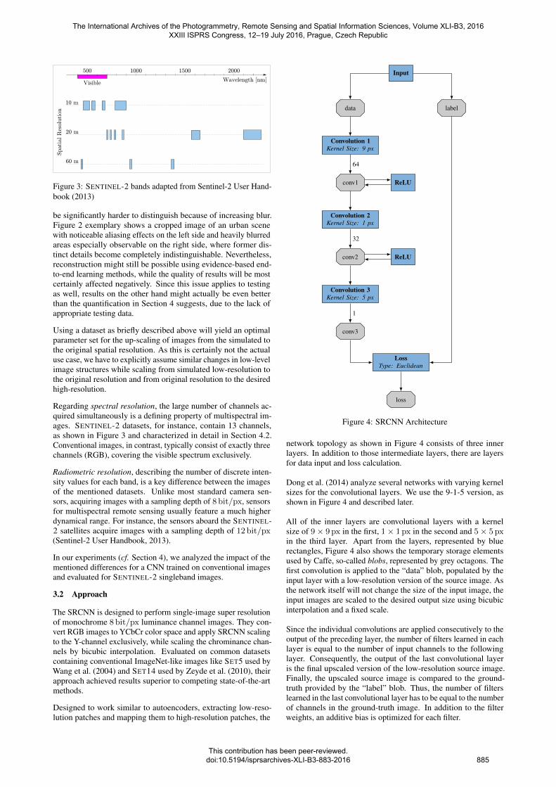
Figure 3: SENTINEL-2 bands adapted from Sentinel-2 User Hand-book (2013)

be significantly harder to distinguish because of increasing blur.Figure 2 exemplary shows a cropped image of an urban scenewith noticeable aliasing effects on the left side and heavily blurredareas especially observable on the right side, where former dis-tinct details become completely indistinguishable. Nevertheless,reconstruction might still be possible using evidence-based end-to-end learning methods, while the quality of results will be mostcertainly affected negatively. Since this issue applies to testingas well, results on the other hand might actually be even betterthan the quantification in Section 4 suggests, due to the lack ofappropriate testing data.

Using a dataset as briefly described above will yield an optimalparameter set for the up-scaling of images from the simulated tothe original spatial resolution. As this is certainly not the actualuse case, we have to explicitly assume similar changes in low-levelimage structures while scaling from simulated low-resolution tothe original resolution and from original resolution to the desiredhigh-resolution.

Regarding spectral resolution, the large number of channels ac-quired simultaneously is a defining property of multispectral im-ages. SENTINEL-2 datasets, for instance, contain 13 channels,as shown in Figure 3 and characterized in detail in Section 4.2.Conventional images, in contrast, typically consist of exactly threechannels (RGB), covering the visible spectrum exclusively.

Radiometric resolution, describing the number of discrete inten-sity values for each band, is a key difference between the imagesof the mentioned datasets. Unlike most standard camera sen-sors, acquiring images with a sampling depth of 8 bit/px, sensorsfor multispectral remote sensing usually feature a much higherdynamical range. For instance, the sensors aboard the SENTINEL-2 satellites acquire images with a sampling depth of 12 bit/px(Sentinel-2 User Handbook, 2013).

In our experiments (cf. Section 4), we analyzed the impact of thementioned differences for a CNN trained on conventional imagesand evaluated for SENTINEL-2 singleband images.

3.2 Approach

The SRCNN is designed to perform single-image super resolutionof monochrome 8 bit/px luminance channel images. They con-vert RGB images to YCbCr color space and apply SRCNN scalingto the Y-channel exclusively, while scaling the chrominance chan-nels by bicubic interpolation. Evaluated on common datasetscontaining conventional ImageNet-like images like SET5 used byWang et al. (2004) and SET14 used by Zeyde et al. (2010), theirapproach achieved results superior to competing state-of-the-artmethods.

Designed to work similar to autoencoders, extracting low-reso-lution patches and mapping them to high-resolution patches, the

Input

data label

Convolution 1Kernel Size: 9 px

conv1 ReLU


conv2 ReLU


conv3

LossType: Euclidean

loss

64

32

1

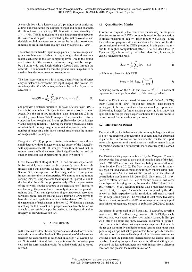
Figure 4: SRCNN Architecture

network topology as shown in Figure 4 consists of three innerlayers. In addition to those intermediate layers, there are layersfor data input and loss calculation.

Dong et al. (2014) analyze several networks with varying kernelsizes for the convolutional layers. We use the 9-1-5 version, asshown in Figure 4 and described later.

All of the inner layers are convolutional layers with a kernelsize of 9× 9 px in the first, 1× 1 px in the second and 5× 5 pxin the third layer. Apart from the layers, represented by bluerectangles, Figure 4 also shows the temporary storage elementsused by Caffe, so-called blobs, represented by grey octagons. Thefirst convolution is applied to the “data” blob, populated by theinput layer with a low-resolution version of the source image. Asthe network itself will not change the size of the input image, theinput images are scaled to the desired output size using bicubicinterpolation and a fixed scale.

Since the individual convolutions are applied consecutively to theoutput of the preceding layer, the number of filters learned in eachlayer is equal to the number of input channels to the followinglayer. Consequently, the output of the last convolutional layeris the final upscaled version of the low-resolution source image.Finally, the upscaled source image is compared to the ground-truth provided by the “label” blob. Thus, the number of filterslearned in the last convolutional layer has to be equal to the numberof channels in the ground-truth image. In addition to the filterweights, an additive bias is optimized for each filter.



885

A convolution with a kernel size of 1 px might seem confusingat first, but considering the number of input and output channels,the filters learned are actually 3D filters with a dimensionality of1× 1× 64. This is equivalent to a non-linear mapping betweenthe low-resolution patterns extracted by the first convolution andthe high-resolution patterns reconstructed by the third convolutionin terms of the autoencoder analogy used by Dong et al. (2014).

The network can handle input image pairs, i.e., source image andground-truth images, of arbitrary size, as long as their dimensionsmatch each other in the loss computing layer. Due to the bound-ary treatment of the network, the source image will be croppedby 12 px in width and height during a forward pass through thenetwork. To compensate for this, the ground-truth image has to besmaller than the low-resolution source image.

The loss layer computes a loss value, quantifying the discrep-ancy or distance between the two input images. The precise lossfunction, called Euclidean loss, evaluated by the loss layer in theSRCNN is

lEucl(θ) =1

2N

N∑n=1

‖F (Dn,θ)− Ln‖22 (1)

and provides a distance similar to the mean squared error (MSE).Here N is the number of images in the currently processed minibatch, D is the set of low-resolution “data” images and L is theset of high-resolution “label” images. The parameter vector θcomprises filter weights and biases applied to the source imagesvia the mapping function F . During the training phase, a so calledmini batch of training images is evaluated in parallel, where thenumber of images in a mini batch is much smaller than the numberof images in the training set.

Dong et al. (2014) propose to train their network on either asmall dataset with 91 images or a larger subset of the ImageNetwith approximately 400 000 images. Since they showed that thetraining results of both datasets differ insignificantly, we used thesmaller dataset in our experiments outlined in Section 4.

Given the results of Dong et al. (2014) and our own experimentsin Section 4.3, we assume that it is generally possible to scaleimages using this network successfully. However, as shown inSection 3.1, multispectral satellite images differ from genericimages in several critical properties. We assume scaling remotesensing images using the same technique is still possible, due tothe fact that the differing properties only affect the parametersof the network, not the structure of the network itself. In end-to-end learning, the parameters in turn only depend on the providedtraining data. Thus, our approach on single-image super resolutionfor multispectral remote sensing data is training a CNN proven tohave the desired capabilities with a suitable dataset. We describethe generation of such dataset in Section 4.2. With using a dataset,matching the test dataset in its properties considerably better, weare able to successfully apply the method to multispectral satelliteimagery, as shown in Section 4.4.

4. EXPERIMENTS

In this section we describe our experiments conducted to verify ourmethods introduced in Section 3. The generation of the dataset weused for our experiments is described in Section 4.2. Section 4.3and Section 4.4 feature detailed descriptions of the evaluation pro-cess and the corresponding results for both the basic and advancedmethod.

4.1 Quantification Metrics

In order to to quantify the results we mainly rely on the peaksignal-to-noise ratio (PSNR), commonly used for the evaluationof image restauration quality. Even though we use the PSNRfor evaluation purposes, it is not used as a loss function for theoptimization of any of the CNNs presented in this paper, mainlydue to its higher computational effort. The euclidean loss, cf.Equation (1), minimized by the solver algorithm, however, isclosely related to the MSE

dMSE =1

N

N∑n=1

(yn − yn)2 (2)

which in turn favors a high PSNR

dPSNR = 10 · log10

(vmax

2

dMSE

)(3)

depending solely on the MSE and vmax = 2b − 1, a constantrepresenting the upper bound of possible intensity values.

Beside the PSNR we evaluated the structural similarity (SSIM)index (Wang et al., 2004) for our test dataset. This measureis designed to be consistent with human visual perception and,since scaling images for further manual processing is an importantapplication for single-image super resolution, this metric seems tobe well suited for our evaluation purposes.

4.2 Multispectral Dataset

The availability of suitable images for training in large quantitiesis a key requirement deep learning in general and our approachin particular. In this section we describe the, for the most partautomatic, generation of a multispectral satellite image datasetfor training and testing our network, more specifically the learnedparameters.

The COPERNICUS programme funded by the European Commis-sion provides free access to the earth observation data of the dedi-cated SENTINEL missions and the contributing missions (Coper-nicus Sentinel Data, 2016). The SENTINEL-2 mission is mainlydesigned for land and sea monitoring through multispectral imag-ing. SENTINEL-2A, the first satellite out of two in the plannedconstellation was launched in June 2015, SENTINEL-2B is ex-pected to follow later in 2016. Each of the two carries or will carrya multispectral imaging sensor, the so called MULTISPECTRALINSTRUMENT (MSI), acquiring images with a radiometric resolu-tion of 12 bit/px. Figure 3 shows the bands acquired by the MSI,as well as their respective spatial resolution. All areas coveredby the acquisition plan will be revisited at least every five days.For our dataset, we used Level-1C ortho-images containing top ofatmosphere reflectances, encoded in 16 bit/px JPEG2000 format.

Our dataset is composed of 75 SENTINEL-2 granules, coveringan area of 100 km2 with an image size of 1980× 1980 px each.We restricted our dataset to five sites mainly located in Europewith little to no cloud and snow coverage, as shown in Figure 5.Since our goal is to show that single-image super resolution tech-niques can successfully applied to remote sensing data rather thangenerating an optimal set of parameters for all possible scenes,this restriction is a reasonable simplification. However to examinewhether or not the parameters learned using our dataset are stillcapable of scaling images of scenes with different settings, weevaluated the learned parameter sets with images from differentlocations and present the results in Section 5.



886

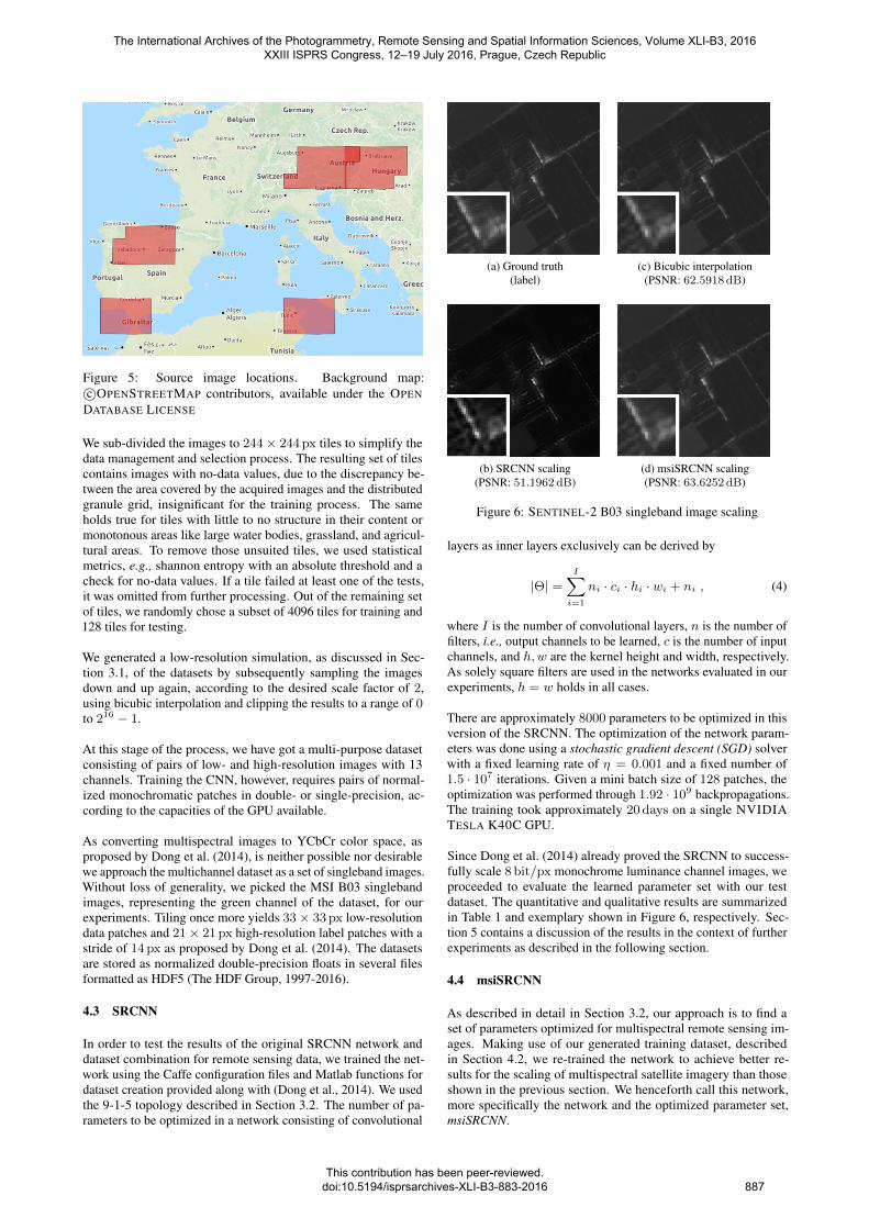
Figure 5: Source image locations. Background map:c©OPENSTREETMAP contributors, available under the OPEN

DATABASE LICENSE

We sub-divided the images to 244× 244 px tiles to simplify thedata management and selection process. The resulting set of tilescontains images with no-data values, due to the discrepancy be-tween the area covered by the acquired images and the distributedgranule grid, insignificant for the training process. The sameholds true for tiles with little to no structure in their content ormonotonous areas like large water bodies, grassland, and agricul-tural areas. To remove those unsuited tiles, we used statisticalmetrics, e.g., shannon entropy with an absolute threshold and acheck for no-data values. If a tile failed at least one of the tests,it was omitted from further processing. Out of the remaining setof tiles, we randomly chose a subset of 4096 tiles for training and128 tiles for testing.

We generated a low-resolution simulation, as discussed in Sec-tion 3.1, of the datasets by subsequently sampling the imagesdown and up again, according to the desired scale factor of 2,using bicubic interpolation and clipping the results to a range of 0to 216 − 1.

At this stage of the process, we have got a multi-purpose datasetconsisting of pairs of low- and high-resolution images with 13channels. Training the CNN, however, requires pairs of normal-ized monochromatic patches in double- or single-precision, ac-cording to the capacities of the GPU available.

As converting multispectral images to YCbCr color space, asproposed by Dong et al. (2014), is neither possible nor desirablewe approach the multichannel dataset as a set of singleband images.Without loss of generality, we picked the MSI B03 singlebandimages, representing the green channel of the dataset, for ourexperiments. Tiling once more yields 33× 33 px low-resolutiondata patches and 21× 21 px high-resolution label patches with astride of 14 px as proposed by Dong et al. (2014). The datasetsare stored as normalized double-precision floats in several filesformatted as HDF5 (The HDF Group, 1997-2016).

4.3 SRCNN

In order to test the results of the original SRCNN network anddataset combination for remote sensing data, we trained the net-work using the Caffe configuration files and Matlab functions fordataset creation provided along with (Dong et al., 2014). We usedthe 9-1-5 topology described in Section 3.2. The number of pa-rameters to be optimized in a network consisting of convolutional

(a) Ground truth(label)

(b) SRCNN scaling(PSNR: 51.1962dB)

(c) Bicubic interpolation(PSNR: 62.5918dB)

(d) msiSRCNN scaling(PSNR: 63.6252dB)

Figure 6: SENTINEL-2 B03 singleband image scaling

layers as inner layers exclusively can be derived by

|Θ| =I∑

i=1

ni · ci · hi · wi + ni , (4)

where I is the number of convolutional layers, n is the number offilters, i.e., output channels to be learned, c is the number of inputchannels, and h,w are the kernel height and width, respectively.As solely square filters are used in the networks evaluated in ourexperiments, h = w holds in all cases.

There are approximately 8000 parameters to be optimized in thisversion of the SRCNN. The optimization of the network param-eters was done using a stochastic gradient descent (SGD) solverwith a fixed learning rate of η = 0.001 and a fixed number of1.5 · 107 iterations. Given a mini batch size of 128 patches, theoptimization was performed through 1.92 · 109 backpropagations.The training took approximately 20 days on a single NVIDIATESLA K40C GPU.

Since Dong et al. (2014) already proved the SRCNN to success-fully scale 8 bit/px monochrome luminance channel images, weproceeded to evaluate the learned parameter set with our testdataset. The quantitative and qualitative results are summarizedin Table 1 and exemplary shown in Figure 6, respectively. Sec-tion 5 contains a discussion of the results in the context of furtherexperiments as described in the following section.

4.4 msiSRCNN

As described in detail in Section 3.2, our approach is to find aset of parameters optimized for multispectral remote sensing im-ages. Making use of our generated training dataset, describedin Section 4.2, we re-trained the network to achieve better re-sults for the scaling of multispectral satellite imagery than thoseshown in the previous section. We henceforth call this network,more specifically the network and the optimized parameter set,msiSRCNN.



887

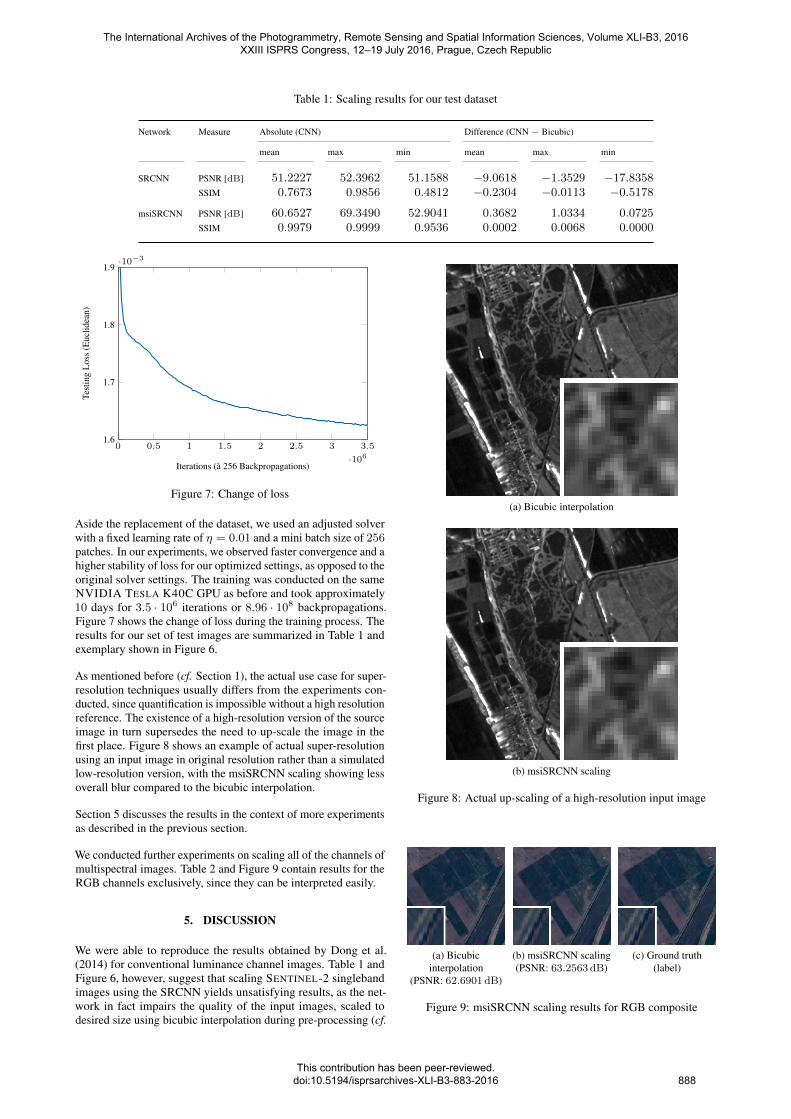
Table 1: Scaling results for our test dataset

Network Measure Absolute (CNN) Difference (CNN − Bicubic)

mean max min mean max min

SRCNN PSNR [dB] 51.2227 52.3962 51.1588 −9.0618 −1.3529 −17.8358SSIM 0.7673 0.9856 0.4812 −0.2304 −0.0113 −0.5178

msiSRCNN PSNR [dB] 60.6527 69.3490 52.9041 0.3682 1.0334 0.0725SSIM 0.9979 0.9999 0.9536 0.0002 0.0068 0.0000

0 0.5 1 1.5 2 2.5 3 3.5

·1061.6

1.7

1.8

1.9·10−3

Iterations (a 256 Backpropagations)

Test

ing

Los

s(E

uclid

ean)

Figure 7: Change of loss

Aside the replacement of the dataset, we used an adjusted solverwith a fixed learning rate of η = 0.01 and a mini batch size of 256patches. In our experiments, we observed faster convergence and ahigher stability of loss for our optimized settings, as opposed to theoriginal solver settings. The training was conducted on the sameNVIDIA TESLA K40C GPU as before and took approximately10 days for 3.5 · 106 iterations or 8.96 · 108 backpropagations.Figure 7 shows the change of loss during the training process. Theresults for our set of test images are summarized in Table 1 andexemplary shown in Figure 6.

As mentioned before (cf. Section 1), the actual use case for super-resolution techniques usually differs from the experiments con-ducted, since quantification is impossible without a high resolutionreference. The existence of a high-resolution version of the sourceimage in turn supersedes the need to up-scale the image in thefirst place. Figure 8 shows an example of actual super-resolutionusing an input image in original resolution rather than a simulatedlow-resolution version, with the msiSRCNN scaling showing lessoverall blur compared to the bicubic interpolation.

Section 5 discusses the results in the context of more experimentsas described in the previous section.

We conducted further experiments on scaling all of the channels ofmultispectral images. Table 2 and Figure 9 contain results for theRGB channels exclusively, since they can be interpreted easily.

5. DISCUSSION

We were able to reproduce the results obtained by Dong et al.(2014) for conventional luminance channel images. Table 1 andFigure 6, however, suggest that scaling SENTINEL-2 singlebandimages using the SRCNN yields unsatisfying results, as the net-work in fact impairs the quality of the input images, scaled todesired size using bicubic interpolation during pre-processing (cf.

(a) Bicubic interpolation

(b) msiSRCNN scaling

Figure 8: Actual up-scaling of a high-resolution input image

(a) Bicubicinterpolation

(PSNR: 62.6901dB)

(b) msiSRCNN scaling(PSNR: 63.2563dB)

(c) Ground truth(label)

Figure 9: msiSRCNN scaling results for RGB composite



888

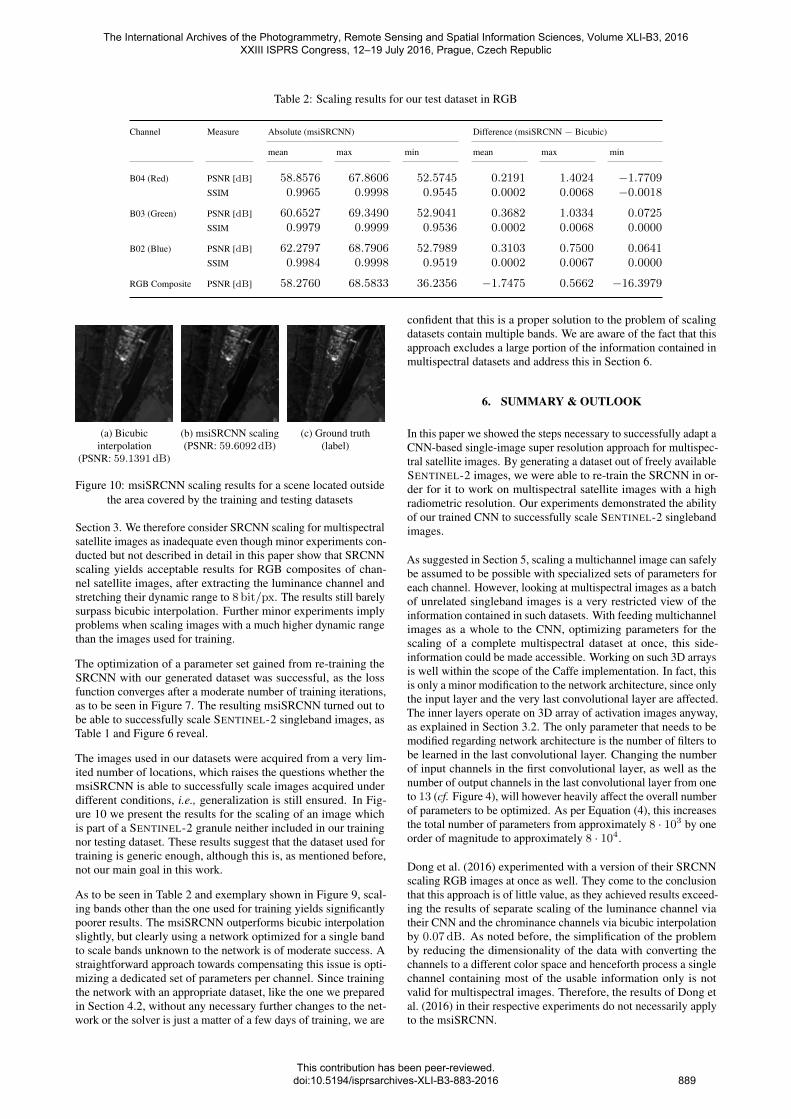
Table 2: Scaling results for our test dataset in RGB

Channel Measure Absolute (msiSRCNN) Difference (msiSRCNN − Bicubic)

mean max min mean max min

B04 (Red) PSNR [dB] 58.8576 67.8606 52.5745 0.2191 1.4024 −1.7709SSIM 0.9965 0.9998 0.9545 0.0002 0.0068 −0.0018

B03 (Green) PSNR [dB] 60.6527 69.3490 52.9041 0.3682 1.0334 0.0725SSIM 0.9979 0.9999 0.9536 0.0002 0.0068 0.0000

B02 (Blue) PSNR [dB] 62.2797 68.7906 52.7989 0.3103 0.7500 0.0641SSIM 0.9984 0.9998 0.9519 0.0002 0.0067 0.0000

RGB Composite PSNR [dB] 58.2760 68.5833 36.2356 −1.7475 0.5662 −16.3979

(a) Bicubicinterpolation

(PSNR: 59.1391dB)

(b) msiSRCNN scaling(PSNR: 59.6092dB)

(c) Ground truth(label)

Figure 10: msiSRCNN scaling results for a scene located outsidethe area covered by the training and testing datasets

Section 3. We therefore consider SRCNN scaling for multispectralsatellite images as inadequate even though minor experiments con-ducted but not described in detail in this paper show that SRCNNscaling yields acceptable results for RGB composites of chan-nel satellite images, after extracting the luminance channel andstretching their dynamic range to 8 bit/px. The results still barelysurpass bicubic interpolation. Further minor experiments implyproblems when scaling images with a much higher dynamic rangethan the images used for training.

The optimization of a parameter set gained from re-training theSRCNN with our generated dataset was successful, as the lossfunction converges after a moderate number of training iterations,as to be seen in Figure 7. The resulting msiSRCNN turned out tobe able to successfully scale SENTINEL-2 singleband images, asTable 1 and Figure 6 reveal.

The images used in our datasets were acquired from a very lim-ited number of locations, which raises the questions whether themsiSRCNN is able to successfully scale images acquired underdifferent conditions, i.e., generalization is still ensured. In Fig-ure 10 we present the results for the scaling of an image whichis part of a SENTINEL-2 granule neither included in our trainingnor testing dataset. These results suggest that the dataset used fortraining is generic enough, although this is, as mentioned before,not our main goal in this work.

As to be seen in Table 2 and exemplary shown in Figure 9, scal-ing bands other than the one used for training yields significantlypoorer results. The msiSRCNN outperforms bicubic interpolationslightly, but clearly using a network optimized for a single bandto scale bands unknown to the network is of moderate success. Astraightforward approach towards compensating this issue is opti-mizing a dedicated set of parameters per channel. Since trainingthe network with an appropriate dataset, like the one we preparedin Section 4.2, without any necessary further changes to the net-work or the solver is just a matter of a few days of training, we are

confident that this is a proper solution to the problem of scalingdatasets contain multiple bands. We are aware of the fact that thisapproach excludes a large portion of the information contained inmultispectral datasets and address this in Section 6.

6. SUMMARY & OUTLOOK

In this paper we showed the steps necessary to successfully adapt aCNN-based single-image super resolution approach for multispec-tral satellite images. By generating a dataset out of freely availableSENTINEL-2 images, we were able to re-train the SRCNN in or-der for it to work on multispectral satellite images with a highradiometric resolution. Our experiments demonstrated the abilityof our trained CNN to successfully scale SENTINEL-2 singlebandimages.

As suggested in Section 5, scaling a multichannel image can safelybe assumed to be possible with specialized sets of parameters foreach channel. However, looking at multispectral images as a batchof unrelated singleband images is a very restricted view of theinformation contained in such datasets. With feeding multichannelimages as a whole to the CNN, optimizing parameters for thescaling of a complete multispectral dataset at once, this side-information could be made accessible. Working on such 3D arraysis well within the scope of the Caffe implementation. In fact, thisis only a minor modification to the network architecture, since onlythe input layer and the very last convolutional layer are affected.The inner layers operate on 3D array of activation images anyway,as explained in Section 3.2. The only parameter that needs to bemodified regarding network architecture is the number of filters tobe learned in the last convolutional layer. Changing the numberof input channels in the first convolutional layer, as well as thenumber of output channels in the last convolutional layer from oneto 13 (cf. Figure 4), will however heavily affect the overall numberof parameters to be optimized. As per Equation (4), this increasesthe total number of parameters from approximately 8 · 103 by oneorder of magnitude to approximately 8 · 104.

Dong et al. (2016) experimented with a version of their SRCNNscaling RGB images at once as well. They come to the conclusionthat this approach is of little value, as they achieved results exceed-ing the results of separate scaling of the luminance channel viatheir CNN and the chrominance channels via bicubic interpolationby 0.07 dB. As noted before, the simplification of the problemby reducing the dimensionality of the data with converting thechannels to a different color space and henceforth process a singlechannel containing most of the usable information only is notvalid for multispectral images. Therefore, the results of Dong etal. (2016) in their respective experiments do not necessarily applyto the msiSRCNN.



889

Au contraire, using the spectral information inherent in each pixeland utilize, e.g., implicit information about the surface material,an extended msiSRCNN is assumed to be able to produce betterresults due to the cross-band information being available. In orderto implement these modifications, some inherent problems needto be solved. The SENTINEL-2 datasets used in our experimentsvary in spatial resolution in their singleband images, as to be seenin Figure 3. Caffe, however, is only able to handle blocks of same-sized input images. Therefore, approaches to this preprocessingsteps, such as scaling the lower-resolution bands to the highestresolution appearing in the dataset using standard interpolationmethods, need to be developed.

To ensure convergence during optimization, a bigger dataset shouldbe used for training, even though our training dataset already out-ranks the dataset successfully used by Dong et al. (2014) in termsof quantity. Certainly, the dataset also has to be extended to amatching number of channels. Our dataset, presented in Sec-tion 4.2, includes all of the 13 spectral bands, thus only the fullyparameterized automatic patch-preparation is affected.

Early stage experiments showed promising results even thoughsome of the mentioned problems still need to be resolved.

ACKNOWLEDGEMENTS

We gratefully acknowledge the support of NVIDIA CORPORA-TION with the donation of the Tesla K40 GPU used for this re-search.

References

Baker, S. and Kanade, T., 2000. Hallucinating faces. In: Proceedingsof the IEEE International Conference on Automatic Face and GestureRecognition (FG), pp. 83–88.

Copernicus Sentinel Data, 2016. https://scihub.copernicus.eu/

dhus, last accessed May 10, 2016.

Deng, J., Dong, W., Socher, R., Li, L. J., Li, K. and Fei-Fei, L., 2009.Imagenet: A large-scale hierarchical image database. In: Proceedingsof the IEEE Conference on Computer Vision and Pattern Recognition(CVPR), pp. 248–255.

Dong, C., Loy, C. C., He, K. and Tang, X., 2014. Learning a deep con-volutional network for image super-resolution. In: D. Fleet, T. Pajdla,B. Schiele and T. Tuytelaars (eds), Proceedings of the European Con-ference Computer Vision (ECCV), Springer International Publishing,Cham, pp. 184–199.

Dong, C., Loy, C. C., He, K. and Tang, X., 2016. Image super-resolutionusing deep convolutional networks. IEEE Transactions on PatternAnalysis and Machine Intelligence (TPAMI) 38(2), pp. 295–307.

Duchon, C. E., 1979. Lanczos filtering in one and two dimensions. Journalof Applied Meteorology 18(8), pp. 1016–1022.

Freeman, W. T., Pasztor, E. C. and Carmichael, O. T., 2000. Learning low-level vision. International Journal of Computer Vision 40(1), pp. 25–47.

Glorot, X., Bordes, A. and Bengio, Y., 2011. Deep sparse rectifier neuralnetworks. In: International Conference on Artificial Intelligence andStatistics (AISTATS), pp. 315–323.

Jia, Y., Shelhamer, E., Donahue, J., Karayev, S., Long, J., Girshick, R.,Guadarrama, S. and Darrell, T., 2014. Caffe: Convolutional architecturefor fast feature embedding. arXiv preprint arXiv:1408.5093.

Krizhevsky, A., Sutskever, I. and Hinton, G. E., 2012. Imagenet clas-sification with deep convolutional neural networks. In: F. Pereira,C. J. C. Burges, L. Bottou and K. Q. Weinberger (eds), Advances inNeural Information Processing Systems 25, Curran Associates, Inc.,pp. 1097–1105.

LeCun, Y., Bengio, Y. and Hinton, G., 2015. Deep learning. Nature521(7553), pp. 436–444.

LeCun, Y., Boser, B., Denker, J. S., Henderson, D., Howard, R. E., Hub-bard, W. and Jackel, L. D., 1989. Backpropagation applied to handwrit-ten zip code recognition. Neural computation 1(4), pp. 541–551.

LeCun, Y., Bottou, L., Bengio, Y. and Haffner, P., 1998. Gradient-basedlearning applied to document recognition. Proceedings of the IEEE86(11), pp. 2278–2324.

Sentinel-2 User Handbook, 2013. https://earth.esa.int/

documents/247904/685211/Sentinel-2_User_Handbook, lastaccessed May 10, 2016.

The HDF Group, 1997-2016. Hierarchical Data Format, version 5. http://www.hdfgroup.org/HDF5/, last accessed May 10, 2016.

Timofte, R., Smet, V. D. and Gool, L. V., 2013. Anchored neighborhoodregression for fast example-based super-resolution. In: Proceedingsof the IEEE International Conference on Computer Vision (ICCV),pp. 1920–1927.

Wang, Z., Bovik, A. C., Sheikh, H. R. and Simoncelli, E. P., 2004. Imagequality assessment: from error visibility to structural similarity. IEEETransactions on Image Processing (IP) 13(4), pp. 600–612.

Yang, J., Wright, J., Huang, T. and Ma, Y., 2008. Image super-resolutionas sparse representation of raw image patches. In: Proceedings ofthe IEEE Conference on Computer Vision and Pattern Recognition(CVPR), pp. 1–8.

Yang, J., Wright, J., Huang, T. S. and Ma, Y., 2010. Image super-resolutionvia sparse representation. IEEE Transactions on Image Processing (IP)19(11), pp. 2861–2873.

Zeyde, R., Elad, M. and Protter, M., 2010. On single image scale-up usingsparse-representations. In: Curves and Surfaces, Springer, pp. 711–730.



890

https://scihub.copernicus.eu/dhus

https://scihub.copernicus.eu/dhus

https://earth.esa.int/documents/247904/685211/Sentinel-2_User_Handbook

https://earth.esa.int/documents/247904/685211/Sentinel-2_User_Handbook

http://www.hdfgroup.org/HDF5/

http://www.hdfgroup.org/HDF5/

single-image super resolution for multispectral remote sensing data … · 2016-06-10 ·...

Documents