single-machine scheduling to minimize the maximum...

Scientia Iranica E (2018) 25(1), 370{385

Sharif University of TechnologyScientia Iranica

Transactions E: Industrial Engineeringhttp://scientiairanica.sharif.edu

Single-machine scheduling to minimize the maximumtardiness under piecewise linear deteriorating jobs

A.A. Jafari and M.M. Lot��

Department of Industrial Engineering, Faculty of Engineering, Yazd University, Yazd, Iran.

Received 9 December 2015; received in revised form 16 October 2016; accepted 25 December 2016

KEYWORDSScheduling;Piecewise lineardeteriorating jobs;Single machine;Tardiness;Branch and Bound;Heuristic.

Abstract. In many realistic production environments, jobs will take longer time if theybegin later. This phenomenon is known as deteriorating jobs which have widely beenstudied. In this paper, the piecewise linear deterioration is discussed in a single-machinescheduling problem of minimizing the maximum tardiness. After proving the NP-hardnessof problem, a Branch and Bound and a heuristic algorithm with O(n2) are proposed tosolve the large-scale problems by near-optimal solutions. The heuristic approach is alsoused to determine an upper bound on the solution of B&B algorithm. The computationalresults of evaluating performance of the two algorithms con�rm the excellent performanceof B&B algorithm as it is able to solve the problems with at least 32 jobs within a reasonabletime. Notably, the heuristic approach is quite accurate and e�cient with an average errorpercentage of less than 0.3%.© 2018 Sharif University of Technology. All rights reserved.

1. Introduction

Nowadays, scheduling problems are applied in di�erentproduction and service systems. In traditional schedul-ing problems, it is assumed that the job processingtimes are known and constant. This assumptionmay not be true for all the cases; there are manysituations in which a job consumes more time whenprocessed later. In fact, when a given job delaysits starting time or waits for process, its processingtime may be increased [1]. In usual, the incrementin processing time is a function of starting time orposition in sequence [2]. These kinds of job are knownas deteriorating jobs, and there is a growing interest tostudy them in the literature.

*. Corresponding author. Tel.: +98 035 31232409;Fax: +98 353 8210699E-mail addresses: [email protected] (A.A. Jafari);lot�@yazd.ac.ir (M.M. Lot�)

doi: 10.24200/sci.2017.4408

Applications of deteriorating jobs can be found inthe �re-�ghting, maintenance planning and scheduling,medical procedures, and searching for an object underworsening weather or growing darkness [1]. Rollingprocess in the steel industries is another well-knowncase of deteriorating jobs. Steel ingots must be heatedup to a predetermined temperature in preheating stage;each ingot rolled earlier has less heat exchange withenvironment and its preheating time will be shorter.Another important application of the above situationis lathing process, in which the needed lathing time willbe increased due to gradual exhaustion of tools [3].

In this paper, Graham symbols [4], in the formof �j�j , is used where �, �, and demonstratemachine environment, problem speci�cation, and ob-jective function, respectively. The variables and pa-rameters used in this paper are described in Table 1.

There is a growing interest in the literatureto study the scheduling problems with deterioratingjobs [5-6]. Alidaee and Womer [7] classi�ed the de-terioration functions into three di�erent kinds: linear,piecewise linear, and non-linear. Most authors assumed

A.A. Jafari and M.M. Lot�/Scientia Iranica, Transactions E: Industrial Engineering 25 (2018) 370{385 371

Table 1. Variables and parameters.Description Notation Description Notation

Number of jobs n Maximum lateness Lmax = maxt�i�nfLtg

ith job ji; i = 1; 2; :::; n Tardiness of ji Ti = maxf0; Ci � digSet of all jobs to be scheduled N = fj1; j2; :::; jng Maximum Tardiness Tmax = max

l�i�nfTigActual processing time of ji Pi; i = 1; 2; :::; n Partial sequence of scheduled jobs �Normal processing time of ji ai; i = 1; 2; :::; n Set of unscheduled jobs (complementary of �) �0

Deterioration rate of ji bi i = 1; 2; :::; n Partial sequence with scheduling ji after � �iStarting time of each job S Maximum tardiness of partial sequence � Tmax(�)

Due date of ji di, i = 1; 2; :::; n Completion time of ji Ci; i = 1; 2; :::; nUi = 0 if di � Ci; otherwise Ui = 1 Ui; i = 1; 2; :::; n Weight of ji wi; i = 1; 2; :::n

Release time of ji ri; i = 1; 2; :::; n Maximum completion time cmax = maxl�i�nfCig

Total completion timePni=1 Ci Weighted total completion time

Pni=1 wiCi

Number of tardy jobs NT =Pni=1 Ui Number of weighted tardy jobs

Pni=1 wiUi

Lateness of ji Li = Ci � di

a linear or piecewise linear deterioration function. Theproblem of deteriorating jobs was reviewed by Chenget al. [8]. They assumed that the processing time ofa job is a linear function of its starting time. In thelinear functions, the deterioration rates may be similaror di�erent. In di�erent deterioration rates, normalprocessing times might be zero or positive. Therefore,the linear deterioration functions are as follows:

Pi = ai + biS; Pi = ai + bS; Pi = biS:

Browne and Yechiali [9] showed that the optimalsequence in problem 1jPi = ai + biSjCmax is basedon non-decreasing rate of ai=bi. Bachman and Janiak[10] proved that problem 1jPi = ai + biSjLmax is NP-complete and presented two heuristics with complexi-ties of O (n:log n) and O(n2). The problem was alsoinvestigated by Hsu and Lin [11] and a Branch andBound (B&B) algorithm was proposed which was ableto solve 100 jobs. Ng et al. [12] proposed a B&Balgorithm for problem F2jPi = ai + biSjPCi whichwas able to handle problems with 15 jobs. Also, theyinvolved a heuristic in the proposed B&B algorithmas an upper bound. Lee et al. [13] consideredproblem FmjPij = aij+bitjPTi and developed a B&Band two metaheuristic algorithms. Yin et al. [14]studied parallel machine scheduling of deterioratingjobs with disruption and presented pseudo-polynomialtime solution algorithms. Luo and Ji [15] consideredsingle-machine scheduling with variable maintenanceunder deteriorating jobs as 1jVM;Pi = ai + biSjCmax,and proved that the problem is NP - hard.

Lee et al. [16] proposed a heuristic and B&B algo-rithm to minimize makespan in a Linear DeterioratingJobs Scheduling Problem (LDJSP) with release time,i.e. 1jPi = ai + bS; ri jCmax; the proposed algorithmsolved problems with 28 jobs. Wu and Lee [17]presented a B&B and several heuristics for problem

F2jPi = ai + biSj�F . The paper was extended byLee et al. [18] and a B&B and several heuristicswere developed to minimize makespan. Jafari andMoslehi [1] proved that problem 1jPi = ai + bS jPUiis NP-hard; hence, a B&B procedure and a heuristicwith O(n2) as an upper bound were proposed. Wangand Wang [19] studied problem F3jPij = aij+bSjCmaxand derived several dominance properties, some lowerbounds and two heuristic algorithms and applied themin a proposed B&B algorithm to �nd the optimalsolution. Yin et al. [20] considered some two-agentsingle-machine scheduling problems with increasinglinear job deterioration and proved their complexity.

The LDJSP with zero normal processing time(Pi = biS) on a single-machine was investigated byMosheiov [21]; he presented the optimal solutionsusing simple rules for performance criteria Cmax,

PCi,P

WiCi, Tmax, Lmax, andPUi. Wang et al. [22]

showed that problem F2jPi = biS jPCi is NP-hard;they proposed a B&B algorithm able to handle 14jobs. Yang and Wang [23] developed a B&B andheuristic algorithm for problem F2jPi = biS jPWiCi.This kind of deterioration function was considered bythe others. Some assumed that the machines are notavailable at any time due to preventive maintenanceor breakdown. For instance, Woo and Lee [24] studiedthe availability constraints on a single machine in tworesumable and non-resumable cases. They proposed aninteger programming model and a heuristic algorithm,respectively, for two problems:

1jr � a; Pi = biS jCmax;

and:

1jnr � a; Pi = biS jXCi:

Some authors supposed that setup time of each jobis not constant; it is a simple linear function of its

372 A.A. Jafari and M.M. Lot�/Scientia Iranica, Transactions E: Industrial Engineering 25 (2018) 370{385

starting time similar to processing time. Cheng etal. [25] presented a B&B algorithm for problem 1jPi =biS; Si = b0iS jTmax. Lee et al. [26] proposed a B&Balgorithm for problem 1jPi = biS; Si = b0iS jPUi whichcould solve the instances up to 1000 jobs in a reasonabletime. Lee and Lu [2] provided a B&B algorithm forproblem 1jPi = biS; Si = b0iS jPWiUi.

Some authors assumed that the deteriorationfunction is piecewise linear in which the actual process-ing time of each job is a function of two or more thantwo constant or linear criteria. Kubiak and Velde [27]studied problem 1jPi jCmax in which Pi is consideredas a non-decreasing three-criteria function as follows:

Pi =

8><>:ai if S � y1

ai + bi(S � y1) if y1 < S < y2

ai + bi(y2 � y1) if S � y2

(1)

where y1 and y2 are the input variables. They showedthat the problem in special case, y2 = 1 and y1 > 0,is NP-hard and proposed a binary B&B algorithm.Moslehi and Jafari [3] surveyed the piecewise lineardeteriorating jobs scheduling problem where the deteri-oration function is similar to Eq. (1) and the objective

is to minimize the number of tardy jobs. They provedthat problem:

1jPi = ai + bi(S � y1); y1 > 0; y2 > y1jnXi=1

Ui;

is NP-hard and developed a B&B procedure and aheuristic algorithm. Lalla Ruiz and Vob [28] consideredproblem PmjPi = ai or ai+bijPCi and presented twomathematical models.

Jafari and Moslehi [29] proved that problem:

1jPi = ai + bi(S � y1); y1 > 0; y2 > y1jnXi=1

Wi Ui;

is NP-hard and provided a B&B algorithm able tohandle 28 jobs. Lai et al. [30] presented the optimalsolutions to a single-machine problem with non-lineardeterioration function. Lee and Yu [31] providedpseudo-polynomial time algorithms to optimize theparallel machine scheduling under potential disruption.

In Table 2, we present a review on the studiesdirected onto the deteriorating jobs scheduling prob-lems where dispatching rule, heuristics, and integer

Table 2. Researches on the deteriorating jobs scheduling problems.

Ref. no. Deterioration function Objective Problem Solutionapproach

[9] Linear (Pi = ai + biS) Cmax 1jPi = ai + biSjCmax DR[10] Linear (Pi = ai + biS) Lmax 1jPi = ai + biSjLmax Heu[11] Linear (Pi = ai + biS) Lmax 1jPi = ai + biSjLmax B&B[12] Linear (Pi = ai + biS)

PCi F2jPi = ai + biSjPCi B&B

[17] Linear (Pi = ai + biS) �F F2jPi = ai + biSj �F B&B, Heu[18] Linear (Pi = ai + biS) Cmax F2jPi = ai + biSjCmax B&B, Heu[16] Linear (Pi = ai + biS) Cmax 1jPi = ai + bS; rijCmax B&B, Heu[1] Linear (Pi = ai + biS)

PUi 1jPi = ai + bSjPUi B&B, Heu

[21] Linear (Pi = biS) Cmax,PCi, 1jPi = biS jCmax 1jPi = biS jPCi DRP

WiCi, 1jPi = biS jPWiCi 1jPi = biS jTmax

Tmax, Lmax,PUi 1jPi = biS jLmax 1jPi = biS jPUi

[22] Linear (Pi = biS)PCi F2jPi = biS jPCi B&B

[23] Linear (Pi = biS)PWiCi F2jPi = biS jPWiCi B&B, Heu

[24] Linear (Pi = biS) Cmax,PCi 1jr � a; Pi = biS jCmax Heu, IP

1jnr � a; Pi = biS jPCi

[25] Linear (Pi = biS) Tmax 1jPi = biS; Si = b0iS jTmax B&B[26] Linear (Pi = biS)

PUi 1jPi = biS; Si = b0iS jPUi B&B

[2] Linear (Pi = biS)PWiUi 1jPi = biS; Si = b0iS jPWiUi B&B

[27] Piecewise Linear Cmax 1jPi = ai + bi(S � y1); y1 > 0; y2 =1jCmax B&B

[3] Piecewise LinearPUi 1jPi = ai + bi(S � y1); y1 > 0; y2 > y1j nP

i=1Ui B&B, Heu

[29] Piecewise LinearPWiUi 1jPi = ai + bi(S � y1); y1 > 0; y2 > y1j nP

i=1Wi Ui B&B

This study Piecewise Linear Tmax 1jPi = ai + bi(S � y1); y1 > 0; y2 > y1jTmax B&B, Heu


programming are shown as DR, HE, and IP, respec-tively.

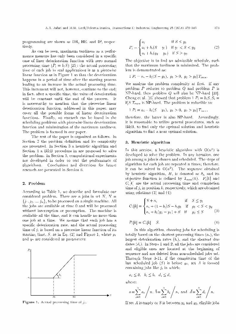
As can be seen, maximum tardiness as a perfor-mance measure has only been considered in a speci�ccase of liner deterioration function with zero normalprocessing time (Pi = biS) [25]; the actual processingtime of each job in real applications is as a piecewiselinear function as in Figure 1 so that the deteriorationhappens in a period of time after the starting processleading to an increase in the actual processing time.This increment will not, however, continue to the end;in fact, after a speci�c time, the value of deteriorationwill be constant until the end of the process. Itis noteworthy to mention that the piecewise lineardeterioration function, addressed in this paper, maycover all the possible forms of linear deteriorationfunctions. Finally, no research can be found in thescheduling problems with piecewise linear deteriorationfunction and minimization of the maximum tardiness.The problem is focused in our paper.

The rest of the paper is organized as follows. InSection 2 the problem de�nition and its complexityare presented. In Section 3 a heuristic algorithm andSection 4 a B&B procedure in are proposed to solvethe problem. In Section 5, computational experimentsare developed in order to test the performance ofalgorithms. Conclusions and directions for futureresearch are presented in Section 6.

2. Problem

According to Table 1, we describe and formulate ourconsidered problem. There are n jobs in set N , N =fj1; j2; :::; jng, to be processed on a single machine. Allthe jobs are available at time 0 and will be processedwithout interruption or preemption. The machine isavailable all the time, and it can handle no more thanone job at a time. We assume that each job has aspeci�c deterioration rate, and the actual processingtime of ji is based on a piecewise linear function of itsstarting time, S, as in Eq. (2) and Figure 1, where y1and y2 are considered as parameters:

Figure 1. Actual processing time of ji.

Pi =

8><>:ai if S � y1

ai + bi(S � y1) if y1 < S < y2

ai + bi(y2 � y1) if S � y2

(2)

The objective is to �nd an admissible schedule, suchthat the maximum tardiness is minimized. The prob-lem is demonstrated as:

1jPi = ai + bi(S � y1); y1 > 0; y2 > y1jTmax:

We analyze the problem complexity at �rst. If anyproblem P reduces to problem Q and problem P isNP-hard, then problem Q will also be NP-hard [32].Cheng et al. [25] showed that problem 1jPi = biS; Si =b0iSjTmax is NP-hard. The problem is reducible to:

1jPi = ai + bi(S � y1); y1 > 0; y2 > y1jTmax;

therefore, the latter is also NP-hard. Accordingly,it is reasonable to utilize general procedures, such asB&B, to �nd only the optimal solution and heuristicalgorithm to �nd a near-optimal solution.

3. Heuristic algorithm

In this section, a heuristic algorithm with O(n2) isdeveloped to solve the problem. In any iteration, onejob among n jobs is chosen and scheduled. The steps ofalgorithm for each job are repeated n times; therefore,it can be solved in O(n2). The sequence obtainedby heuristic algorithm, H, is denoted as �h and itsobjective function is de�ned by Tmax(h). Pi[k] andCi[k] are the actual processing time and completiontime of ji in position k, respectively, which are obtainedusing relations (3) and (4):

Ci[k] =

8><>:S + ai if S � y1

ai + (1 + bi)S � biy1 if y1 < S < y2

ai + bi(y2 � y1) + S if y2 � S (3)

Pi[k] = Ci[k]� S: (4)

In this algorithm, choosing jobs for scheduling istotally based on the shortest processing times (ai), thelargest deterioration rates (bi), and the shortest duedates (di). In Steps 1 and 2, all the jobs are consideredand eligible ones are located at the beginning ofsequence and are deleted from non-scheduled jobs set.Through Steps 3-11, if the completion time of thelast scheduled job (S) is before y1, set A is formedcontaining jobs like ji in which:

ai � �a; bi � �b; di � �d;

where:

�a=nXi=1

ai

,n; �b=

nXi=1

bi

,n; and �d=

nXi=1

di

,n:

If set A is empty or S is between y1 and y2, eligible jobs


are chosen from the set of unscheduled jobs accordingto Steps 12 and 14. In Step 16, if S is greater thany2, then non-scheduled jobs are arranged based on theEDD rule and scheduled at the end of scheduled jobs.The steps of algorithm H are as follows:

- Step 0. Start. Set k = 1, L = fj1; j2; :::; jng, A = �,S = 0, Tmax = 0.

- Step 1. If:

ji 2 L;ai = minf

j2Lajg; bi = maxf

j2Lbjg;

di = minfj2L

djg S + ai � y1;

then go to Step 2; else, go to Step 3.- Step 2. Schedule ji in position k and calculate Ci[k].

Set S = Ci[k], L = L�ji, and k = k+1. If k = n+1,then go to Step 16; else, go to Step 1.

- Step 3. Calculate:

a =nXi=1

ai=n; b =nXi=1

bi=n

and d =nXi=1

di=n:

- Step 4. If S < y1, then set A is updated based onthe following condition:

For ji 2 L :

if ai � a; bi � b; and di � d;then

A = A+ ji:

- Step 5. If A = �, go to Step 6; else, go to Step 9.- Step 6. If S < y1, then set A is updated based on

the following condition:

For ji 2 L :

if ai � a and bi � bthen

A = A+ ji:

If A = �; go to Step 7; else, go to Step 9:


For ji 2 L :

if ai � a and di � dthen

A = A+ jj



For ji 2 L :

if bi � b and di � dthen

A = A+ ji:


- Step 9. If A = � and S < y1, then go to Step 6.If S � y1, go to Step 14; else, choose ji withthe smallest ai from A and schedule it in the kthposition. Set S = Ci[k], L = L� ji, A = A� ji, andk = k + 1. If k = n + 1, then go to Step 16; else,repeat Step 9.

- Step 10. If S � y1, then go to Step 14; else, for allthe jobs ji 2 L, if di � �d, then set A = A+ ji.

- Step 11. If A = �, then go to Step 12; else, chooseji with the smallest ai

bi and the largest bi from A, setA = A � ji and go to Step 13. If there is no sucha job, then choose ji with the largest bi from A, setA = A� ji, and go to Step 13.

- Step 12. Choose ji with the smallest aibi and largest

bi from L and go to Step 13. If there is no such ajob, then choose ji with the largest bi from L and goto Step 13.

- Step 13. Schedule ji in position k. Set S = Ci[k],L = L � ji, and k = k + 1. If k = n + 1, then goto Step 16; if S < y1, then go to Step 11; else, go toStep 14.

- Step 14. If S � y2, then go to Step 15; else, chooseji 2 L with one of the following conditions and goto Step 13:� ji has the smallest ai=bi and smallest di;� ji has the largest bi and smallest di;� ji has the smallest ai=bi and largest bi;� ji has the smallest ai and smallest di;� ji has the smallest bi and smallest di;� ji has the smallest ai;� ji has the largest bi.

- Step 15. Sequence unscheduled jobs by the EDD


rule from k to n.

1. Step 16. Denote the �nal sequence as �h and itsobjective function as Tmax(h), respectively.

4. B&B algorithm

In this section, a B&B algorithm using the back-tracking strategy is proposed to search for the optimalsolution where upper bound, lower bounds, and domi-nance rules are used in an e�cient manner. At �rst, weestablish several dominance rules to fathom the search-ing tree, and then present a property to determinethe ordering of remaining jobs (set �0). In addition,three lower bounds are provided in Subsection 4.3. Inthe proposed B&B algorithm, when a job from set �0is selected for scheduling, its involvement in set � ischecked by dominance rules and lower bounds. If it isnot fathomed, then it will be added to the end of set �.

4.1. Upper boundIn this paper, heuristic algorithm H is considered asthe upper bound of problem and its �nal sequence (�h)will be a basis for generating the searching tree.

4.2. Dominance rulesDominance rules are important in solving the schedul-ing problems. In this subsection, some dominanceproperties are given to be employed in the B&Balgorithm. It is assumed that partial sequence, �, withcompletion time, S, and maximum tardiness, Tmax(�),is in hand. If ji is processed immediately after partialsequence, �, then the resulted sequence is shown as �iand if jj is located after �i, then the sequence will beshown by �ij. Notably, partial sequence �ji is the resultof pairwise interchange of ji and jj in partial sequence�ij. To show that �ij dominates �ji, one should provethat Tmax(�ij) � Tmax(�ji) and Cj(�ij) � Ci(�ji).

Completion times of ji and jj in partial sequence�ij are as follows:

Ci(�ij) =

8><>:S + ai if S � y1

ai + (1 + bi)S � biy1 if y1 < S < y2

ai + bi(y2 � y1) + S if y2 � S (5)

Cj(�ij) =8><>:S + aj + ai if Ci(�ij) � y1

aj + (1 + bj)Ci(�ij)� bjy1 if y1 < Ci(�ij) < y2

aj + bj(y2 � y1) + Ci(�ij) if y2 � Ci(�ij) (6)

Lemma 1. In problem 1jPi = ai + bi(S � y1); y1 >0; y2 > y1jTmax, the jobs completed before y1 will bearranged by the EDD rule.

Proof. The actual processing time of jobs completedbefore y1 is constant. Hence, the problem would belike the basic form 1jTmax where sequence based on theEDD rule is optimal; therefore, completed jobs beforey1 will be arranged by the EDD rule.

Lemma 2. In problem 1jPi = ai + bi(S � y1); y1 >0; y2 > y1jTmax, if S > y1 and the following relationshold, then there exists an optimal sequence in which jimust be processed before jj :

y2 � ai + S(1 + bi)� biy1; (7)

y2 � aj + S(1 + bj)� bjy1; (8)

ai + aj + aibj + (S � y1)(bi + bj + bibj) + S � dj� Tmax(�); (9)

aj + aibj + (S � y1)(bj + bibj) + di � dj ; (10)

ai + aj + ajbi + (S � y1)(bi + bj + bibj) + S � di� Tmax(�); (11)

ai + ajbi + (S � y1)(bi + bibj) + dj � di; (12)

dj � aibj � ajbi + di; (13)

aj/bj � ai/bi: (14)

Proof. Since S > y1, y2 � ai + S(1 + bi)� biy1, andy2 � aj + S(1 + bj) � bjy1, the completion times of jiand jj in �ij and �ji are as follows:

Ci(�ij) = ai + (1 + bi)S � biy1; (15)

Cj(�ij)=ai+aj+aibj+(S�y1)(bi+bj+bibj)+S;(16)

Cj(�ji) = aj + (1 + bj)S � bjy1; (17)

Ci(�ji)=ai+aj+ajbi+(S�y1)(bi+bj+bibj)+S:(18)

From aj/bj � ai/bi, it implies that:

Ci(�ji) � Cj(�ij): (19)

According to the de�nition of tardiness and max-imum tardiness, we have the following relations:

Ti(�ij) = maxf0; ai + (1 + bi)S � biy1 � dig; (20)

Tj(�ij) = maxf0; ai + aj + aibj

+ (S � y1)(bi + bj + bibj) + S � djg; (21)

Tj(�ji) = maxf0; aj + (1 + bj)S � bjy1 � djg; (22)


Ti(�ji) = maxf0; ai + aj + ajbi

+ (S � y1)(bi + bj + bibj) + S � dig; (23)

Tmax(�ij) = maxfTmax(�); Ti(�ij); Tj(�ij)g; (24)

Tmax(�ji) = maxfTmax(�); Ti(�ji); Tj(�ji)g: (25)

Due to Relations (9), (10), and (24), the followingrelation is satis�ed:

Tmax(�ij) = Tj(�ij): (26)

Also, Relations (11), (12), and (25) express that thefollowing relation is valid:

Tmax(�ji) = Ti(�ji): (27)

Relation (13) shows that Ti(�ji) � Tj(�ij): So, we havethe following relation:

Tmax(�ji) � Tmax(�ij): (28)

Based on Relations (19) and (28), we can con�rmthat sequence �ij dominates sequence �ji, and thus theproof is completed.


y2 � ai + S(1 + bi)� biy1; (29)

y2 � aj + S(1 + bj)� bjy1; (30)

Tmax(�) � ai + S(1 + bi)� biy1 � di; (31)

Tmax(�) � ai + aj + aibj + (S � y1)(bi + bj + bibj)

+ S � dj ; (32)

Tmax(�) � aj + S(1 + bj)� bjy1 � dj ; (33)

Tmax(�) � ai + aj + ajbi + (S � y1)(bi + bj + bibj)

+ S � di; (34)



y2 � ai + S(1 + bi)� biy1; (36)

y2 � aj + S(1 + bj)� bjy1; (37)

Tmax(�) � ai + S(1 + bi)� biy1 � di; (38)

Tmax(�) � ai + aj + aibj + (S � y1)(bi + bj + bibj)

+ S � dj ; (39)

ai + aj + ajbi + (S � y1)(bi + bj + bibj)

+ S � di � Tmax(�); (40)




y2 � ai + S(1 + bi)� biy1; (43)

y2 � aj + S(1 + bj)� bjy1; (44)

ai + S(1 + bi)� biy1 � di � Tmax(�); (45)

dj � aj + aibj + (S � y1)(bj + bibj) + di; (46)

ai + aj + ajbi + (S � y1)(bi + bj + bibj)

+ S � di � Tmax(�); (47)



Notably, the proofs of Lemmas 3 to 5 are omittedsince they are similar to that of Lemma 2. However,they are available upon the request of the interestedreaders. We present Lemma 6 to determine theordering of jobs in set �0 and to further speed upsearching process.

Lemma 6. In problem 1jPi = ai + bi(S � y1); y1 >0; y2 > y1jTmax, if S � y2, then the optimal sequenceafter y2 will be obtained by using EDD rule on set �0as follows.

Proof. After y2, actual processing time of jobs inset �0 is known and constant so that the problemis equivalent to problem 1jjTmax in which optimalsequence is obtained via EDD rule. So, jobs startedafter y2 should be arranged by EDD rule.

Lemma 7. In problem 1jPi = ai + bi(S � y1); y1 >

0; y2 > y1j nPi=1

Ui , if there exists ji so that relations


ai = minfj2�0

ajg, bi = maxfj2�0

bjg, di = minfj2�0

djg, and

S + ai � y1 hold, then there always exists an optimalsequence in which ji is scheduled at time S.

Proof. As ji has the least normal process time, itwill have shortest completion time and starting andprocessing times of the following jobs will becomeshorter. Also, the selection of ji makes the job with thelargest deterioration rate be scheduled in a conditionthat there would not be any deterioration for it. Itwould make the next jobs have less deterioration andthe shortest completion time. On the other hand, jihas the least due date; so, scheduling it on time S willnot increase the maximum tardiness.

As a result, employing the above lemma at thestart of each algorithm may lead to scheduling thejobs at the beginning and omit them from set Nwhose search space of problem is reduced. In addition,implementing the lemma in depth search process ofB&B algorithm leads to the selection of the best jobfrom set �0; so, there is no need to search the otherbranches.

4.3. Lower boundsLower bounds can further enhance the e�ciency ofB&B algorithm. In each node, the objective functionof partial sequence � is Tmax(�) and its lower bound isshown by LB�. In order to obtain LB�, the followingtheorems are presented.

Theorem 1. In partial sequence � for problem 1jPi =ai+bi(S�y1); y1 > 0; y2 > y1jTmax, if all the jobs in set�0 are scheduled one by one at time S, then lower boundLB1 is obtained according to the following relation:

LB1 = maxfTmax(�); max8i2�0f0; Ci(�i)� digg: (50)

Proof. Obviously, any di�erent sequence of jobs inset �0 will have no e�ect on Tmax(�). Also, schedulinga given job in set �0 at time S leads to one of thefollowing two cases for that job. If the job becomestardy at time S, then its tardiness will increase afterS; in contrast, if the job does not become tardy attime S, then its tardiness will not decrease after S.Hence, maximum tardiness of set �0 will never be lessthan max8i2�0f0; Ci(�i)�dig. Therefore, the objectivefunction of each complete sequence would not be lessthan LB1.

Theorem 2. In partial sequence � for problem 1jPi =ai + bi(S� y1); y1 > 0; y2 > y1jTmax, lower bound LB2is calculated as follows:

LB2 = maxfTmax(�); Tmax(�0EDD) g; (51)

where Tmax(�0EDD) is obtained according to EDD rulefor the jobs in set �0 assuming deterioration at time Sfor each job.

Proof. Any arbitrary sequence of jobs in set �0 willhave no impact on Tmax(�). Furthermore, it is apparentthat the actual processing time and completion time ofeach job assuming the deterioration at time S is nothigher than the real deterioration. Since the maximumtardiness in basic form 1jjTmax is optimized via EDDrule, by relaxing the assumption of real deteriorationand using the deterioration at time S for all the jobs inset �0, the maximum tardiness will never be less thanTmax(�0EDD). Hence, the objective function of eachcomplete sequence will not be less than LB2.

Theorem 3. In partial sequence � for problem 1jPi =ai + bi(S� y1); y1 > 0; y2 > y1jTmax, lower bound LB3is calculated by the following relation:

LB3 = maxfTmax(�); Tmax(�0LB)g; (52)

where Tmax(�0LB) is calculated by algorithm LB.

Algorithm LB

- Step 0. Set Tmax = 0, C = S, M = 1, k = 1, �0 =fj1; j2; :::; jug, NT (�0) = 0, B�0 = fb�0[1]; b

�0[2]; :::; b

�0[u]g,

and D�0 = fd�0[1]; d�0[2]; :::; d

�0[u]g, such that b�

0[1] � b�

0[2] �

::: � b�0

[u] and d�0

[1] � d�0

[2] � ::: � d�0

[u]g where u is thenumber of jobs in set �0.

- Step 1. Choose a job with the least aj from set�0 and schedule it at time C. If C � y1, then setC = C + aj , M = M + 1, �0 = �0 � jj and go toStep 2; else, select M deterioration rates from setD�0 and assign them to M scheduled jobs at the endof sequence in a non-increasing order; then, calculatetheir completion times. Set C = Cj , M = M + 1,and �0 = �0 � jj .

- Step 2. If C � d[k] � Tmax, then k = k + 1 and goto step 3; else, set Tmax = C� d[k], k = k+ 1 and goto Step 1.

- Step 3. If k � u, then go to Step 1; else, setTmax(�0LB) = Tmax.

Proof. The proof of Theorem 3 is presented in theAppendix.

The lower bound for every node of B&B tree iscalculated by the following relation:

LB� = maxfLB1; LB2; LB3g: (53)


5. Computational experiments

In this section, a set of random generated test problemsis considered in order to evaluate the performance ofB&B and heuristic algorithms. The test problems weresolved on a Pentium 4 PC with 2.53 GHz CPU and 3GRAM under Windows XP. In the following subsections,the problem generation procedure and analysis of theresults are described. Notably, the intervals of uniformdistribution for the test problem parameters are similarto those of [3].

5.1. Test problemsThe normal processing times (ai) and deteriorationrates (bi) are randomly generated from discrete uni-form distribution over (0; 10] and continuous uniformdistribution over (0; 1], respectively. y1 and y2 arealso generated from continuous uniform distributionsover intervals [0; A=3] and [0; 2A=3] for y1 and intervals[A=3; 2A=3] and [2A=3; A] for y2, where A is assumedto be determined as in:

A =nXi=1

ai:

As y2 > y1, in order to generate values of y1 and y2,three distinctive conditions for di�erent combinationsof y1 and y2 would be logical. Due dates were alsogenerated randomly from continuous uniform distribu-tions over (0; 0:5Cmax], [0:5Cmax; Cmax], (0; Cmax], and(0; 1:5Cmax] where Cmax is makespan of the obtainedsequence based on the non-decreasing ratio of ai=bi.For the number of jobs (n), values of 8, 12, 16,20, 24, 28, 32, 36, 40, and 44 were utilized [3].Considering the intervals of y1, y2, and due date, 12groups, S111 to S224, were formed whose de�nitionsand speci�cations are brie y given in Table 3. For anypossible combination of S111 to S224 and n, 20 testproblems were randomly generated. Accordingly, 2400(i.e., 12�10�20) sample problems were generated andsolved totally.

5.2. Computational resultsHeuristic procedure H and B&B algorithm were codedin C++ and sample problems were solved. In ourB&B method, a time limit equal to 4000 seconds foreach problem was considered; if a problem does notget the optimal solution in this limitation, then B&Bprocedure will be stopped. In Table 4, computationalresults for 12 groups of problems are presented. Asobserved in Table 4, the optimal solution is achievedfor all the sample problems with at least 32 jobs.Moreover, some sample problems with more jobs arealso solved.

In order to study the performance of heuristicapproach, the error percentages based on the followingequation are recorded:

Table 3. Speci�cations of the di�erent groups ofproblems.

No Range of deteriorationfunction variables

Range of due dates

y2 y1

1 [A=3; 2A=3] [0; A=3] (0; :5Cmax]2 [A=3; 2A=3] [0; A=3] [:5Cmax; Cmax]3 [A=3; 2A=3] [0; A=3] (0; Cmax]4 [A=3; 2A=3] [0; A=3] (0; 1:5Cmax]5 [2A=3; A] [0; A=3] (0; :5Cmax]6 [2A=3; A] [0; A=3] [:5Cmax; Cmax]7 [2A=3; A] [0; A=3] (0; Cmax]8 [2A=3; A] [0; A=3] (0; 1:5Cmax]9 [2A=3; A] [0; 2A=3] (0; :5Cmax]10 [2A=3; A] [0; 2A=3] [:5Cmax; Cmax]11 [2A=3; A] [0; 2A=3] (0; Cmax]12 [2A=3; A] [0; 2A=3] (0; 1:5Cmax]

%Error = (Z � Z�)/Z� � 100 %;

where Z and Z� are Tmax obtained from heuristicalgorithm and optimal schedule, respectively.

In Table 4, average and maximum values of%Error are presented. The corresponding columnshows that the average %Error is less than 0.3% whichproves that the proposed heuristic algorithm is highlyaccurate; therefore, solving the large-scale problemsis recommended. Notably, the computation time ofheuristic algorithm is not recorded since it is almost�nished in zero time.

As can be seen in Table 4, the performance ofB&B algorithm is di�erent for 12 groups; it signi�-cantly depends upon the values of due dates, y1 andy2. As the maximum tardiness in the problems withlarge due dates is lower than the maximum tardinessin those with short due dates, a great decrease in thenumber of nodes happens, which results in the easyproblems. Generally, large values of y1 cause a decreasein the completion times of jobs because jobs do nothave any deterioration up to time y1. Decreasing thecompletion times of jobs leads to an increase in thenumber of utilization of the dominance rules and lowerbounds, especially LB3; so, it makes the problems hardto solve. Large values of y2 also bring about an increasein the quantity of employing the lemmas and theorems.According to Lemma 8, on the other hand, obtainingthe optimal solution for small values of y2 is easier thanthat for large values; hence, large values of y2 make theproblems di�cult.

The results given in Table 4 indicate that themaximum job size, whose B&B method is able to solve,is 44 belonging to groups S114, S124, and S224. Figure 2demonstrates the minimum average of CPU times for


Table 4. Performance of B&B and heuristic algorithms.

Gro

up

n

# ofoptimumsamples

% Error

AvgCPU

time ofB&B (s)

%Avg of fathomed nodes by

%Avg ofall

fathomednodes

B&B H Avg Max Lema 6 Lem 1 Lem 7 Lem 2 Lem 3 Lem 4 Lem 5 LB3 LB1 LB2

S111

8 20 15 0.09 0.43 0.00 4.49 1.30 1.27 4.37 0.21 1.50 3.19 76.02 2.91 4.74 97.04

12 20 12 0.11 0.56 0.02 8.63 1.26 2.61 2.13 2.97 1.77 2.64 65.88 4.70 7.41 97.89

16 20 12 0.09 0.60 0.12 13.59 0.48 1.86 2.55 3.49 2.94 4.19 59.13 4.45 7.32 99.07

20 20 10 0.05 0.34 1.42 14.45 2.62 4.12 1.95 2.92 1.62 2.30 58.07 5.14 6.81 91.81

24 20 6 0.08 0.70 32.82 15.52 0.35 3.64 0.95 1.85 1.32 3.22 59.86 4.70 8.59 91.84

28 20 7 0.05 0.12 293.03 12.41 0.32 4.37 1.12 1.65 3.03 2.01 63.67 6.88 4.53 95.81

32 20 6 0.07 0.68 1072.02 16.82 0.47 5.41 2.25 8.49 2.08 2.55 50.59 5.18 6.17 92.12

36 12 5 0.04 0.19 1000.25 11.21 0.58 1.37 1.61 2.81 1.43 3.14 66.13 6.18 5.54 94.27

S112

8 20 16 0.05 0.35 0.00 10.98 1.00 3.06 0.76 0.32 0.99 0.78 76.53 1.72 3.85 98.66

12 20 13 0.24 1.24 0.00 13.85 1.98 1.43 0.45 0.14 0.41 3.11 74.78 0.24 3.62 96.23

16 20 12 0.13 0.59 0.04 11.64 3.01 2.17 1.33 0.01 0.75 0.59 76.66 1.66 2.17 88.26

20 20 7 0.15 1.09 0.37 21.36 2.15 1.73 0.54 0.08 2.28 1.66 64.33 1.59 4.29 94.41

24 20 8 0.11 0.98 2.64 30.54 1.51 0.74 1.14 0.81 1.65 1.36 59.76 1.18 1.30 90.52

28 20 6 0.04 0.44 28.93 26.17 2.35 1.32 0.14 1.36 0.00 0.94 66.38 0.49 0.85 84.63

32 20 4 0.03 0.37 100.04 34.24 5.39 4.51 0.09 0.21 0.05 1.48 51.83 0.09 2.11 95.72

36 20 5 0.09 1.03 725.82 22.07 3.68 2.96 0.85 1.91 1.24 2.66 61.43 1.27 1.93 89.61

40 17 4 0.06 0.36 2154.78 14.71 3.65 0.92 1.45 0.56 1.37 2.51 72.73 0.94 1.16 93.53

S113

8 20 13 0.08 0.34 0.00 7.31 1.77 2.10 0.79 0.35 1.81 1.86 69.44 4.04 10.52 97.40

12 20 18 0.01 0.12 0.01 8.50 1.52 1.16 1.21 1.45 4.86 2.84 66.33 4.40 7.73 96.06

16 20 14 0.11 1.75 0.09 8.14 2.15 2.50 1.76 2.26 0.70 3.50 64.54 6.33 8.13 90.93

20 20 9 0.29 4.67 0.54 21.05 2.23 5.19 0.53 2.31 0.55 2.70 55.06 5.59 4.80 92.54

24 20 7 0.02 0.22 6.27 16.25 1.35 4.25 0.69 0.85 0.87 1.29 61.91 4.35 8.19 91.84

28 20 4 0.07 1.16 45.18 25.24 4.21 6.12 1.16 1.20 2.25 3.41 46.61 5.12 4.68 93.35

32 20 1 0.06 0.91 116.26 28.25 2.65 3.84 0.44 0.94 1.69 2.45 50.48 4.12 5.14 92.68

36 20 2 0.04 0.24 650.33 24.38 1.24 4.45 1.96 2.21 1.78 2.84 50.75 6.55 3.84 94.74

40 11 1 0.18 1.22 1327.30 18.96 1.09 3.75 1.66 1.95 1.09 2.85 59.80 4.43 4.42 95.60

S114

8 20 18 0.04 0.62 0.00 2.45 0.84 1.25 0.65 0.12 0.26 1.26 86.54 4.24 2.38 91.24

12 20 15 0.18 1.66 0.00 3.45 2.28 2.20 1.21 2.14 0.05 0.61 73.65 5.42 8.99 90.76

16 20 10 0.06 0.48 0.11 8.65 1.24 0.65 0.23 0.72 0.42 1.45 76.78 3.11 6.75 90.14

20 20 11 0.00 0.05 0.86 6.24 0.92 0.89 0.76 0.64 0.13 0.83 80.34 6.87 2.38 94.56

24 20 6 0.03 0.12 1.27 10.65 0.00 1.40 1.62 1.14 0.42 1.14 76.84 4.24 2.55 93.37

28 20 5 0.01 0.08 3.94 12.65 0.68 0.36 0.85 0.81 0.92 0.35 70.23 3.51 9.64 90.27

32 20 3 0.02 0.11 15.13 6.84 1.21 1.02 1.32 0.41 0.19 0.65 78.21 2.54 7.61 89.77

36 20 4 0.02 0.06 95.58 8.54 2.12 1.86 0.65 0.67 1.81 1.32 68.58 5.51 8.94 92.76

40 20 1 0.00 0.06 435.41 7.79 3.24 2.47 0.34 1.42 0.68 1.55 72.12 3.61 6.78 94.78

44 20 2 0.04 0.09 1650.96 7.12 1.04 0.95 0.00 0.89 0.44 0.59 77.34 4.42 7.21 94.24

S121

8 20 16 0.04 0.49 0.00 2.24 2.43 2.35 1.34 1.47 2.93 1.62 74.86 4.21 6.55 94.43

12 20 16 0.06 0.97 0.00 3.82 0.65 4.57 2.61 2.73 4.61 2.05 67.22 3.43 8.31 95.67

16 20 11 0.05 0.35 1.12 8.56 2.54 3.49 2.02 2.12 2.14 1.68 62.37 4.34 10.74 86.34

20 20 8 0.05 0.27 8.44 7.44 1.14 6.73 1.33 2.37 3.08 2.94 60.64 6.94 7.39 96.72

24 20 4 0.00 0.04 35.82 9.32 1.36 8.41 3.76 1.43 2.59 2.57 59.44 4.30 6.82 95.07

28 20 5 0.01 0.11 455.67 10.65 0.85 0.24 2.45 3.74 1.68 1.44 66.18 5.86 6.91 90.51

32 20 3 0.02 0.21 2890.83 7.74 1.73 16.37 2.76 2.47 2.34 3.51 46.52 8.23 8.33 94.92

36 16 1 0.00 0.01 1850.19 6.96 2.38 2.61 3.27 4.70 1.11 2.73 66.19 4.63 5.42 84.20

8 20 15 0.08 0.74 0.00 3.29 2.41 1.81 0.04 1.45 0.98 0.57 88.58 0.41 0.46 92.42aLem: Lemma.


Table 4. Performance of B&B and heuristic algorithms (continued).

Gro

up

n

# ofoptimumsamples

% Error

AvgCPU

time ofB&B (s)


%Avg ofall

fathomednodes


S122

12 20 12 0.05 0.61 0.08 2.43 3.63 1.75 0.69 0.75 2.37 1.65 84.10 1.69 0.94 94.61

16 20 13 0.12 1.05 0.48 6.74 1.54 2.59 0.88 1.70 1.67 2.37 80.49 0.75 1.27 96.45

20 20 10 0.19 1.16 1.22 3.81 0.98 1.97 0.96 0.42 1.76 1.93 86.18 0.60 1.39 88.26

24 20 5 0.06 0.91 14.48 8.56 2.12 1.24 0.41 1.34 2.58 0.71 79.22 1.37 2.45 93.20

28 20 5 0.11 1.35 110.33 8.12 3.58 1.48 0.65 0.97 0.64 0.95 81.36 0.00 2.25 92.42

32 20 2 0.21 0.45 866.89 4.97 2.91 1.13 0.29 1.94 2.37 1.84 82.15 1.43 0.97 94.18

36 20 3 0.09 0.81 2154.78 5.93 0.41 0.92 1.27 1.02 1.13 2.08 84.95 0.82 1.47 90.04

S123

8 20 16 0.06 0.90 0.00 6.35 0.96 0.24 1.21 2.51 1.55 1.20 75.18 4.60 6.20 94.18

12 20 12 0.11 1.58 0.00 4.57 2.64 0.83 0.84 1.57 0.95 2.67 77.82 3.99 4.12 96.28

16 20 13 0.18 2.13 0.03 5.14 1.43 0.92 1.70 2.63 1.82 1.13 77.08 2.19 5.96 90.59

20 20 8 0.02 0.30 0.67 3.68 1.76 0.81 0.36 0.97 0.80 2.19 79.99 5.86 3.58 95.66

24 20 3 0.09 0.45 44.15 2.27 2.39 0.81 1.22 1.84 1.02 0.87 78.45 4.77 6.36 88.74

28 20 3 0.03 0.06 180.55 5.69 3.72 0.60 1.95 1.22 0.93 2.55 74.04 3.51 5.79 93.62

32 20 1 0.02 0.12 428.91 6.12 1.87 0.51 0.72 0.97 1.24 0.72 78.09 4.84 4.92 94.93

36 20 2 0.08 0.10 712.25 4.71 2.44 0.88 2.42 1.41 2.79 0.42 71.48 5.26 8.19 89.67

40 12 2 0.04 0.08 950.56 6.91 3.26 0.69 0.63 1.22 1.75 1.94 75.19 4.69 3.72 92.25

S124

8 20 16 0.02 0.11 0.00 3.47 1.32 0.69 0.98 1.41 1.27 0.94 80.05 3.11 6.76 90.99

12 20 15 0.03 0.16 0.00 4.66 1.45 0.46 1.38 1.18 2.84 0.65 74.44 2.56 10.38 94.24

16 20 13 0.04 0.12 0.00 3.19 2.34 0.04 1.75 0.94 0.73 1.28 77.06 3.96 8.71 92.35

20 20 9 0.00 0.01 0.02 4.21 1.54 0.42 0.84 0.00 0.49 0.78 80.45 4.81 6.46 96.03

24 20 11 0.00 0.02 0.09 7.96 2.34 0.00 2.76 1.09 1.65 2.34 69.69 4.62 7.55 88.27

28 20 7 0.00 0.00 6.94 2.35 1.84 0.09 0.54 1.54 0.49 0.71 83.36 5.89 3.19 93.14

32 20 5 0.00 0.03 34.43 8.58 0.97 0.01 1.89 0.43 1.38 1.22 78.55 4.21 2.76 87.42

36 20 5 0.01 0.08 147.81 6.41 1.23 0.00 1.19 1.89 0.91 1.07 71.99 5.37 9.94 92.86

40 20 6 0.00 0.04 675.92 7.80 2.43 0.87 0.97 2.01 1.00 2.63 73.93 4.54 3.82 96.24

44 14 2 0.01 0.12 1348.76 8.28 1.89 0.93 1.65 2.18 1.11 2.78 76.16 2.90 2.12 93.64

S221

8 20 14 0.09 1.44 0.00 5.44 2.65 0.75 1.94 2.66 1.35 2.58 75.32 4.93 2.38 93.72

12 20 10 0.04 0.63 0.05 6.17 4.78 1.32 1.47 0.91 2.51 3.24 64.06 6.55 8.99 97.39

16 20 11 0.07 1.09 0.67 3.30 2.40 1.54 2.05 1.23 0.97 2.85 73.67 5.24 6.75 92.03

20 20 5 0.08 1.39 4.66 3.86 3.13 0.68 2.69 2.12 6.62 2.62 66.46 4.93 6.90 88.55

24 20 9 0.04 0.65 25.72 9.64 2.12 2.95 1.27 1.46 3.06 3.20 55.74 8.63 11.93 97.23

28 20 6 0.12 0.21 185.93 4.79 8.89 1.49 1.38 0.00 1.28 2.77 66.03 3.18 10.18 88.58

32 20 4 0.01 0.04 620.55 5.29 4.72 0.70 2.53 2.75 2.40 6.89 57.26 5.58 11.88 93.08

36 18 3 0.01 0.18 1497.07 5.94 6.55 3.88 1.40 2.08 2.58 2.50 60.35 4.30 10.43 84.56

40 9 3 0.00 0.01 675.66 2.25 7.63 4.27 2.72 1.67 3.67 1.65 66.27 3.45 6.42 92.61

S222

8 20 12 0.12 1.48 0.00 1.45 1.92 2.85 0.82 0.96 1.16 0.89 83.44 5.36 1.15 98.76

12 20 10 0.09 1.36 0.00 5.81 4.68 2.48 1.04 1.63 2.42 0.64 72.20 3.14 5.96 94.92

16 20 7 0.06 0.97 0.21 6.91 3.61 3.47 1.61 1.55 1.45 1.60 69.68 7.31 2.81 94.81

20 20 8 0.11 1.72 3.51 4.34 7.36 0.92 0.94 2.84 1.59 2.32 75.73 1.92 2.04 96.57

24 20 5 0.14 0.98 68.35 8.57 4.71 1.55 1.21 0.60 1.71 2.60 69.64 2.74 6.67 89.29

28 20 2 0.16 1.50 1243.76 2.70 3.12 2.67 0.74 1.54 0.54 1.77 80.20 3.55 3.17 90.67

32 20 3 0.11 0.76 2875.88 6.32 4.07 5.09 1.35 1.01 1.92 1.53 68.12 5.14 5.45 88.25

36 10 0 0.09 0.56 1562.93 4.18 3.71 2.42 1.55 0.96 1.38 2.50 74.47 4.65 4.18 91.73

8 20 13 0.00 0.03 0.00 3.47 2.47 1.27 0.88 1.33 1.34 1.38 74.60 7.94 5.32 94.48

12 20 14 0.13 0.90 0.01 7.96 3.54 1.46 0.73 4.34 1.05 2.80 65.29 10.23 2.59 96.85aLem: Lemma.


Table 4. Performance of B&B and heuristic algorithms (continued).

Gro

up

n

# ofoptimumsamples

% Error

AvgCPU

time ofB&B (s)


%Avg ofall

fathomednodes


S223

16 20 8 0.09 1.03 0.53 5.27 1.38 0.58 1.31 1.10 1.48 1.32 77.08 3.78 6.69 94.4620 20 4 0.06 0.61 3.98 4.52 4.10 2.73 0.00 2.75 2.00 0.93 69.20 6.65 7.11 90.1324 20 3 0.00 0.02 84.62 5.29 6.21 1.29 0.61 4.23 0.95 2.03 68.73 8.39 2.27 85.8928 20 5 0.16 0.86 198.94 6.15 5.97 2.11 1.54 3.12 2.63 2.83 63.09 3.64 8.92 95.3132 20 0 0.08 0.34 822.50 3.88 2.02 0.93 0.84 2.68 3.54 3.20 74.96 4.50 3.45 91.4336 15 2 0.03 0.28 1100.50 4.24 2.96 0.67 0.62 3.71 2.01 1.79 74.86 4.96 4.18 93.59

S224

8 20 17 0.02 0.38 0.00 6.10 1.25 1.07 0.84 0.99 2.38 2.29 78.34 5.62 1.12 98.8612 20 11 0.01 0.09 0.07 4.22 2.55 0.93 1.23 1.16 1.57 1.41 76.37 5.89 4.67 89.2116 20 13 0.00 0.05 0.15 3.67 1.47 2.49 0.66 1.64 1.16 0.00 83.05 3.45 2.41 96.5820 20 9 0.00 0.01 1.45 7.51 4.18 2.13 1.05 1.28 3.83 2.40 68.48 2.90 6.24 93.7824 20 5 0.00 0.01 5.63 4.13 3.09 1.37 0.76 0.86 1.40 5.08 73.07 3.69 6.55 93.0728 20 7 0.00 0.00 3.49 10.27 7.62 2.55 1.47 0.89 2.07 0.95 64.06 6.22 3.90 84.9632 20 4 0.00 0.00 2.28 7.38 3.48 0.78 2.04 3.05 0.95 2.67 71.18 4.31 4.16 85.5836 20 1 0.00 0.02 146.10 4.80 5.67 1.63 0.66 2.01 0.65 1.22 74.38 6.93 2.05 91.4540 20 1 0.01 0.11 910.59 6.58 2.19 1.79 0.43 1.39 2.93 0.67 78.20 4.21 1.61 88.7844 20 3 0.00 0.02 1985.68 5.16 1.49 2.02 1.23 1.60 2.62 1.84 77.53 4.64 1.87 93.63

aLem: Lemma.

Figure 2. Average CPU time of B&B algorithm.

solving the three groups in which the values of duedate are generated over the wide interval (0; 1:5Cmax],although values of y1 and y2 in S224 are large. Also,groups S111, S121, and S221 have large CPU times andsmall solved job sizes; due dates of those groups wereobtained over small range (0; 0:5Cmax]. In addition,because of the longest interval of y1 and y2 values ingroups S221 and S223, the average CPU times of solvingthe generated hard problems are rather high. Since y1and y2 in group S222 were generated over the longestinterval and due dates were obtained over the shortinterval (0:5Cmax; Cmax], this group is strongly hard tosolve; the maximum CPU time and minimum numberof optimal samples belong to this group as given inTable 4 and Figure 3.

In Table 4, the e�ciency of all the lemmas andlower bounds is also demonstrated by the averagepercentage of fathomed nodes presented according tothe order of accomplishment in B&B algorithm. Dueto having the shortest interval of y2 over [A=3; 2A=3]in the groups S111, S112, and S113, the number of

Figure 3. Number of optimal samples obtained by B&Balgorithm.

utilizing Lemma 6 is increased and the performance ofthis lemma is great. Also, in groups S221, S222, S223,and S224, where y1 is obtained from the longest interval[0; 2A=3], Lemma 1 is highly e�cient.

According to Table 4, the e�ciency of LB3 isso excellent in all the groups; in many problems, itfathoms the initial nodes of B&B tree so that thenumerous branches of searching tree, and thus a greatpercentage of entire nodes are omitted. As it canbe seen, due to having large due dates over intervals(0:5Cmax; Cmax] and (0; 1:5Cmax] in S112, S114, S122,S124, S222, and S224, the e�ciency of LB1 and LB2 isdecreased. The average percentage of fathomed nodesis at least 84% which proves a fantastic performance ofthe proposed B&B method.

6. Conclusion and future research

In this paper, the single-machine scheduling problem


under piecewise linear deteriorating jobs was investi-gated whose objective is to minimize the maximumtardiness. It was assumed that the processing timeof jobs is an increasing function of their starting timeaccording to a piecewise linear function. The problemis known to be NP-hard; therefore, a B&B algorithmwith several dominance rules and lower bounds wasestablished to solve the problem optimally. A heuristicmethod was also proposed to derive the near-optimalsolutions. The experimental results showed a highperformance of the proposed B&B algorithm as it couldsolve the problems with at least 32 jobs in 12 di�erentgroups. Furthermore, it was shown that the averagepercentage error of heuristic approach is less than 0.3%which demonstrates its great capabilities to solve thelarge-scale problems. Scheduling problem under deteri-orating jobs is an interesting topic for research studies.The future studies may focus on multiple machinesor the other objective functions. Furthermore, somepractical assumptions, such as the machine availabilityconstraint or release times, might be added. Also,the other types of deterioration function, such as theexponential form with the assumption of learning orforgetting e�ects, can be investigated.

References

1. Jafari, A. and Moslehi, G. \Scheduling linear deteri-orating jobs to minimize the number of tardy jobs",Journal of Global Optimization, 54(2), pp. 389-404(2012).

2. Lee, WC. and Lu, Z.S. \Group scheduling with dete-riorating jobs to minimize the total weighted numberof late jobs", Applied Mathematics and Computation,218(17), pp. 8750-8757 (2012).

3. Moslehi, G. and Jafari, A. \Minimizing the numberof tardy jobs under piecewise-linear deterioration",Computers & Industrial Engineering, 59(4), pp. 573-584 (2010).

4. Pinedo, M., Scheduling: Theory, Algorithms, andSystems, 3th Ed., Upper Saddle River, Prentice Hall(2002).

5. Yin, Y., Cheng, T.C.E. and Wu, C.C. \Scheduling withtime-dependent processing times 2015\, MathematicalProblems in Engineering, Article ID 367585, 2 pages(2015).

6. Yin, Y., Cheng, T.C.E. and Wu, C.C. \Schedulingwith time-dependent processing times", MathematicalProblems in Engineering, Article ID 201421, 2 pages(2014).

7. Alidaee, B. and Womer, N.K. \Scheduling with timedependent processing times: Review and extensions",Journal of the Operational Research Society, 50(7), pp.711-720 (1999).

8. Cheng, T.C.E., Ding, Q. and Lin, B.M.T. \A concisesurvey of scheduling with time-dependent processingtimes", European Journal of Operational Research,152(1), pp. 1-13 (2004).

9. Browne, S. and Yechiali, U. \Scheduling deterioratingjobs on a single processor", Computers & OperationsResearch, 38(3), pp. 495-498 (1990).

10. Bachman, A. and Janiak, A. \Minimizing maximumlateness under linear deterioration theory and method-ology", European Journal of Operational Research,126(3), pp. 557-566 (2000).

11. Hsu, Y.S. and Lin, B.M.T. \Minimization of maximumlateness under linear deterioration", Omega, 31(6), pp.459-469 (2003).

12. Ng, C.T., Wang, J.B., Cheng, T.C.E. and Liu, L.L. \Abranch-and-bound algorithm for solving a two-machine ow shop problem with deteriorating jobs", Computers& Operation Research, 37(1), pp. 83-90 (2010).

13. Lee, W.C., Yeh, W.C. and Chung, Y.H. \Total tar-diness minimization in permutation owshop with de-terioration consideration", Applied Mathematical Mod-elling, 38(13), pp. 3081-3092 (2014).

14. Yin, Y., Wang, Y., Cheng, T.C.E., Liu, W. and Li, J.\Parallel-machine scheduling of deteriorating jobs withpotential machine disruptions", Omega, 69, pp. 17-28(2017).

15. Luo, W., and Ji, M. \Scheduling a variable mainte-nance and linear deteriorating jobs on a single ma-chine", Information Processing Letters, 115, pp. 33-39(2015).

16. Lee, W.C., Wu, C.C. and Chung, Y.H. \Schedulingdeteriorating jobs on a single machine with releasetimes", Computers & Industrial Engineering, 54(3),pp. 441-452 (2008).

17. Wu, C.C. and Lee, W.C. \Two-machine owshopscheduling to minimize mean ow time under lineardeterioration", International Journal of ProductionEconomics, 103(2), pp. 572-584 (2006).

18. Lee, W.C., Wu, C.C., Wen, C.C. and Chung, Y.H.\A two-machine owshop makespan scheduling prob-lem with deteriorating jobs", Computers & IndustrialEngineering, 54(4), pp. 737-749 (2008).

19. Wang, J.B. and Wang, M.Z. \Minimizing makespanin three-machine ow shops with deteriorating jobs",Computers & Operation Research, 40(2), pp. 547-557(2013).

20. Yin, Y., Cheng, T.C.E., Wan, L., Wu, C.C. and Liu,J. \Two-agent single-machine scheduling with deterio-rating jobs", Computers & Industrial Engineering, 81,pp. 177-185 (2015).

21. Mosheiov, G. \Scheduling jobs under simple linear de-


terioration", Computers & Operation Research, 21(6),pp. 653-659 (1994).

22. Wang, J.B., Ng, C.T.D., Chen, T.C.E. and Liu,L.L. \Minimizing total completion time in a two-machine ow shop with deteriorating jobs", AppliedMathematics and Computation, 180(1), pp. 185-193(2006).

23. Yang, S.H. and Wang, J.B. \Minimizing total weightedcompletion time in a two-machine ow shop schedulingunder simple linear deterioration", Applied Mathemat-ics and Computation, 217(9), pp. 4819-4826 (2011).

24. Wu, C.C. and Lee, W.C. \Scheduling linear deterio-rating jobs to minimize makespan with an availabilityconstraint on a single machine", Information Process-ing Letters, 87(2), pp. 89-93 (2003).

25. Cheng, T.C.E., Hsu, C.J., Huang, Y.C. and Lee, W.C.\Single-machine scheduling with deteriorating jobsand setup times to minimize the maximum tardiness",Computers & Operation Research, 38(12), pp. 1760-1765 (2011).

26. Lee, W.C., Lin, J.B. and Shiau, Y.R. \Deterioratingjob scheduling to minimize the number of late jobs withsetup times", Computers & Industrial Engineering,61(3), pp. 782-787 (2011).

27. Kubiak, W. and Velde, S. \Scheduling deterioratingjobs to minimize makespan", Naval Research Logistics,45(5), pp. 511-523 (1998).

28. Lalla Ruiz, E. and Vob, S. \Modeling the parallel ma-chine scheduling problem with step deteriorating jobs",European Journal of Operational Research, 255(1), pp.21-33 (2016).

29. Jafari, A. and Moslehi, G. \Minimizing the weightednumber of tardy jobs on a single machine under piece-wise linear deterioration", 9th International IndustrialEngineering Conference, Tehran, Iran (2013).

30. Lai, P., Wu, C. and Lee, W. \Single machine schedul-ing with logarithm deterioration", Optimization Let-ters, 6(8), pp. 1719-1730 (2011).

31. Lee, C. and Yu, G. \Parallel machine scheduling underpotential disruption", Optimization Letters, 2(1), pp.27-37 (2008).

32. Brucker, P. Scheduling Algorithm, 5th Ed., Heidelberg,Berlin (2006).

Appendix

Proof of Theorem 3: Tmax(�0LB) in algorithm LB isbased on comparing the least completion time for eachposition after partial sequence � to the best possibledue date (Steps 1 and 2). At �rst, we show thatif non-decreasing ratio of ai=ab is observed for eachposition, M , after partial sequence, �, then the shortestcompletion time for position M is obtained. Then, weprove that if this completion time is compared to theleast existing due date, LB3 is a lower bound for thisproblem.

Let �1 = (�; �; ji; jj) where � and � are partialsequences with completion times S and C, and i and jare located in positions M�1 and M after �. Sequence�2 = (�; �; jj ; ji) is obtained from �1 by interchanging jiand jj . To show that the shortest completion time forposition M is based on non-decreasing ratio of ai=bi, wemust show that ai=bi � aj=bj to have Cj(�1) � Ci(�2).According to Relation (2), completion times of ji andjj in �1 are as follows:

Ci(�1) =

8><>:C + ai if C � y1

ai + bi(C � y1) + C = ai+(1 + bi)C�biy1 if y1<C � y2 (A.1)

If Ci(�1) < y2, then completion time of jj in �1 is asfollows:

Cj(�1) = aj + bj(Ci(�1)� y1) + Ci(�1)

= aj + bj(ai + (1 + bi)C � biy1 � y1)

+ ai + (1 + bi)C � biy1

= aj + aibj + bj(1 + bi)C � bibjy1 � bjy1 + ai

+ (1 + bi)C � biy1: (A.2)

Now, if Ci(�1) > y2, then completion time of jj in �1is as follows:

Cj(�1) = aj + bj(y2 � y1) + Ci(�1)

= aj + bj(y2 � y1) + ai + (1 + bi)C � biy1:(A.3)

Also, completion times of ji and jj in �2 are as follows:

Cj(�2) =

8><>:C + aj if C � y1

aj + bj(C � y1) + C = aj + (1 + bj)C � bjy1 if y1 < C � y2 (A.4)

If Cj(�2) < y2, then completion time of jj in �1 is asfollows:

Ci(�2) = ai + bi(Cj(�2)� y1) + Cj(�2)

= ai + bi(aj + (1 + bj)C � bjy1 � y1)

+ aj + (1 + bj)C � bjy1

= ai + biaj + bi(1 + bj)C � bibjy1 � biy1 + aj

+ (1 + bj)C � bjy1: (A.5)

Now, if Cj(�2) > y2, then completion time of jj in �1is as follows:

Ci(�2) = ai + bi(y2 � y1) + Cj(�2)


= ai + bi(y2 � y1) + aj + (1 + bj)C � bjy1: (A.6)

According to the completion time of ji and jj ,there are four cases to prove Theorem 3 that need tobe checked one by one.

Case 1: Ci(�1) < y2 and Cj(�2) < y2:

Cj(�1)� Ci(�2) = (aj + aibj + bj(1 + bi)C

� bibjy1 � bjy1 + ai + (1 + bi)C � biy1)

� (ai + biaj + bi(1 + bj)C � bibjy1 � biy1

+ aj + (1 + bj)C � bjy1)

= aj + aibj + bjC + bibjC � bibjy1 � bjy1

+ ai + C + biC � biy1 � ai � biaj � biC� bibjC + bibjy1 + biy1 � aj � C � bjC + bjy1

= aibj � biaj : (A.7)

Since Cj(�1) � Ci(�2) � 0, we have aibj � biaj � 0.Therefore, it implies that ai=bi � aj=bj .

Case 2: Ci(�1) < y2 and Cj(�2) > y2:

Cj(�1)� Ci(�2) = (aj + aibj + bj(1 + bi)C � bibjy1

� bjy1 + ai + (1 + bi)C � biy1)� (ai

+ bi(y2 � y1) + aj + (1 + bj)C � bjy1)

= aj + aibj + bjC + bibjC � bibjy1 � bjy1

+ ai + C + biC � biy1 � ai � biy2 + biy1 � aj� C � bjC + bjy1

= aibj + bibjC � bibjy1

+ biC � biy2: (A.8)

From Ci(�1) < y2, we obtain the following relation:

aibj + bibjC � bibjy1 + biC � biy2 � aibj + bibjC

� bibjy1 + biC � biCi(�1): (A.9)

If the right-hand side of Inequality (A.9) is not positive,then the left-hand side will not be positive. Thus, thefollowing relation is valid:

aibj + bibjC � bibjy1 + biC � biCi(�1) = aibj

+ bibjC�bibjy1+biC�bi(ai+(1 + bi)C � biy1)

� 0;

aibj + bibjC � bibjy1 + biC � biai� biC � bi2C + bi2y1

= bj(ai + biC � biy1)

� bi(ai + biC � biy1)

� 0;

bj(ai + biC � biy1)

� bi(ai + biC � biy1);

bj � bi: (A.10)

On the other hand, from relations Ci(�1) < y2 andy2 < Cj(�2), we have Ci(�1) < Cj(�2):

ai + (1 + bi)C � biy1 < aj + (1 + bj)C � bjy1;

ai + biC � biy1 < aj + bjC � bjy1;

ai � aj < (bj � bi)C�(bj�bi)y1 =(bj � bi)(C � y1):(A.11)

Owing to bj � bi and y1 < C, relation (bj � bi)(C �y1) � 0 and, consequently, ai < aj hold. Accordingly,we have ai=bi � aj=bj .Case 3: Ci(�1) > y2 and Cj(�2) < y2:

Cj(�1)� Ci(�2) = (aj + bj(y2 � y1) + ai + (1 + bi)C

� biy1)� (ai + biaj + bi(1 + bj)C � bibjy1

� biy1 + aj + (1 + bj)C � bjy1)

= aj + bjy2 � bjy1 + ai + C + biC � biy1

� ai � biaj � biC � bibjC + bibjy1 + biy1

� aj � C � bjC + bjy1

= bjy2 � biaj � bibjC+ C + biC � biy1 � ai � biy2 + biy1 � aj+ bibjy1 � bjC: (A.12)

Since Ci(�1) > y2, we can replace Ci(�1) with y2:


bjy2 � biaj � bibjC + bibjy1 � bjC < bjCi(�1)

� biaj � bibjC + bibjy1 � bjC= bj(ai + C + biC � biy1)� biaj� bibjC + bibjy1 � bjC= bjai � biaj : (A.13)

Cj(�1)�Ci(�2) � 0; therefore, relations aibj� biaj � 0and ai=bi � aj=bj are satis�ed.

Case 4: Ci(�1) > y2 and Cj(�2) > y2:

Cj(�1)� Ci(�2) = (aj + bj(y2 � y1) + ai + (1

+ bi)C � biy1)� (ai + bi(y2 � y1) + aj

+ (1 + bj)C � bjy1)

= bj(y2 � C) + bi(C � y2)

= (bj � bi)(y2 � C): (A.14)

Since we want to have Cj(�1) � Cj(�2) � 0, wehave (bj � bi)(y1 � C) � 0. From C � y2, we obtainbj < bi. While the shortest normal processing time (ai)is used in Relation (A.1), the least amount of Ci(�1) inposition M is obtained. Therefore, relation ai � aj issatis�ed. Consequently, we have ai=bi � aj=bj .

In the above four cases, we proved that non-decreasing ratio ai=bi causes to have the least comple-tion time for each position. If the start time of positionis before y1, then ratio ai=bi is reduced to ai. Accordingto Step 1 of algorithm LB, the least amount of ai fromset �0 is selected and scheduled, then it will be omittedfrom �0. If the start time is greater than y1 (e.g.,position M), then the shortest ai remained in set �0(e.g., aj) is scheduled for this position so that ai � aj .To ensure non-decreasing ratio of ai=bi, relation bj < bimust hold; so, M jobs with the least deterioration ratesfrom set B�0 are chosen and scheduled in positions 1 toM after � in a non-increasing order. Then, completiontime of job in position M is calculated according to thecompletion times of the previous positions.

We showed how to obtain the least completiontime of each position based on the non-decreasing ratioof ai=bi so far. Now, we prove that if the least existingdue date is assigned to each opposition, the lowerbound will be obtained. We have:

Tmax(�0LB) = max1�k�uf0; C[k] � d[k]g

= maxf0; C[1] � d[1]; C[2] � d[2]; C[3]

� d[3]; :::; C[u] � d[u]g; (A.15)where C[k] is the least completion time of position k,and d[k] is the kth smallest due date from set D�0 .

Suppose that there is a number 1 � h � u inpartial sequence �0LB so that Tmax(�0LB) = C[h] � d[h].There is partial sequence �0 where d[h] is not assignedto position h; hence, there is a number 1 � k � u,so that d[h] � d[k] or d[k] < d[h] where d[h] and d[k]are assigned to positions k and h, respectively. SinceTmax(�0LB) = C[h]�d[h], relations C[k]�d[k] � C[h]�d[k]and Tmax(�0) � maxfC[h] � d[k] � C[k] � d[h]g hold.

If d[h] � d[k], then relation h < k is satis�edabsolutely. Therefore, we have:

C[h] < C[k];

C[h] � d[h] < C[k] � d[h]

Tmax(�0LB) = C[h] � d[h] < C[k] � d[h] � Tmax(�0);

Tmax(�0LB) � Tmax(�0): (A.16)

If d[k] < d[h], then the following relation is satis�ed:

Tmax(�0LB) = C[h] � d[h] < C[h] � d[k] � Tmax(�0);

Tmax(�0LB) � Tmax(�0): (A.17)

Therefore, partial sequence �0LB dominates partial se-quence �0. Accordingly, LB3 is a lower bound for theproblem.

Biographies

Abbas-Ali Jafari is a PhD candidate at the De-partment of Industrial Engineering at Yazd University.He received his BS degree from Yazd University andhis MS degree from Isfahan University of Technology,both in Iran. One of his main �eld of interest is thescheduling and production planning.

Mohammad Mehdi Lot� is an Associate Professorat the Department of Industrial Engineering at YazdUniversity. He received his BS degree from SharifUniversity of Technology and his MS and PhD degreesfrom University of Tehran, all in Iran. One of his mainareas of interest is the production planning, schedulingand control in operation systems.

single-machine scheduling to minimize the maximum...

Documents