1

Supporting Information

To

Single-Molecule Dynamics of the Molecular Chaperone Trigger Factor in Living Cells

Feng Yang, Tai-Yen Chen, Łukasz Krzemiński, Ace George Santiago, Won Jung, and Peng

Chen*

Department of Chemistry and Chemical Biology, Cornell University, Ithaca, New York, 14853, U.S.A.

*Corresponding author: pc252@cornell.edu

Table of Contents S1. Constructs and strains ............................................................................................................................. 3

S1.1 General molecular biology procedures ............................................................................................. 3 S1.2 Construction of the C-terminal tagged chromosomal TF gene with mEos3.2 via λ-Red homologous recombination ....................................................................................................................... 3 S1.3 Construction of pBAD24_TF-mEos3.2 plasmid and pET21b_TF-mEos3.2 plasmid ...................... 4 S1.4 Construction of pBAD24_TF*-mEos3.2 plasmid ............................................................................ 4 S1.5 Construction of pBAD24_Ffh plasmid ............................................................................................. 4 S1.6 Construction of photoconvertible bimolecular fluorescence complementation (PC-BiFC) constructs .................................................................................................................................................. 5

S1.6.1 General information about PC-BiFC constructs ........................................................................ 5 S1.6.2 Construction of mEos3.2-fragment-tagged fusion genes ........................................................... 5 S1.6.3 Procedures for making pETDuet-1 plasmids for co-expression ................................................ 6 S1.6.4 Procedures for making three pBAD constructs for functional assay ......................................... 6

S2. Intactness and functionality of mEos3.2 and mEos3.2-fragment tagged TF in E. coli........................... 9 S2.1 Protein gel analyses show mEos3.2 and mEos3.2-fragment tagged TF stay intact inside cells ....... 9

S2.1.1 Coomassie-Blue stained SDS-PAGE shows TFmE is intact as a fusion protein inside cells at overexpression level .............................................................................................................................. 9 S2.1.2 Western blot further shows TFmE is intact as a fusion protein at basal expression level and the mE fusion tag does not change its expression from the chromosomal locus ........................................ 9 S2.1.3 Coomassie-Blue stained SDS-PAGE shows mEos3.2-fragment tagged TF are intact at overexpression level ............................................................................................................................ 10

S2.2 Cell growth assays under SDS/EDTA stress show that mEos3.2 and mEos3.2-fragment tagged TF are functional .......................................................................................................................................... 12

S3. Microscopy cell sample preparation ..................................................................................................... 13 S4. Imaging setup for single-molecule tracking (SMT) via time-lapse stroboscopic imaging and for single-cell quantification of protein concentration (SCQPC) in living cells .............................................. 14

2

S4.1 Microscope configuration ............................................................................................................... 14 S4.2 Single-molecule tracking (SMT) via time-lapse stroboscopic imaging .......................................... 15 S4.3 Single-cell quantification of protein concentration (SCQPC) ........................................................ 16 S4.4 PALM imaging of fixed cells (strains containing leucine zipper constructs) ................................. 17

S5. Single-molecule localization and tracking data analysis ...................................................................... 17 S5.1 Determination of single-molecule locations ................................................................................... 17 S5.2 Generation of SMT trajectories ...................................................................................................... 19

S6. Determination of the number of diffusion states as well as their diffusion constants and fractional populations .................................................................................................................................................. 19

S6.1 Probability density function (PDF) and cumulative distribution function (CDF) of displacement length r per time lapse ............................................................................................................................. 19 S6.2 Validation of diffusion state analysis using hidden Markov model ................................................ 22 S6.3 Validation of diffusion state analysis using inverse transformation of the confined displacement distribution (ITCDD) method ................................................................................................................. 23

S7. Determination of unbinding kinetics of TF from the 70S ribosome ..................................................... 24 S7.1 Determination of photobleaching/blinking kinetics of mEos3.2 in E. coli cells ............................ 24 S7.2 Determination of the photobleaching/blinking corrected unbinding rate constant of TF from the 70S ribosome .......................................................................................................................................... 25 S7.3 Validation of the unbinding kinetics analysis via changing the threshold r0 and hidden Markov model analysis ......................................................................................................................................... 25

S7.3.1 Varying r0 to make the integrated area ratio between D2 and D3 population below the threshold in PDF be the same and repeat the kinetics analysis ........................................................... 25 S7.3.2 Validation of the kinetics analysis using hidden Markov model ............................................. 25

S8. Spatial distribution analysis of TF in living cells ................................................................................. 26 S8.1 Uncovering the clustering of TFs using the probability distribution of pairwise distances ............ 26

S8.1.1 General procedures of pairwise distance analysis ................................................................... 26 S8.1.2 Pairwise distance analyses of TFmE

FRK/AAA and TF2mE do not show the existence of clusters;

whereas the analysis of TF2,ΔC13mE does .............................................................................................. 27

S8.2 Distribution of TF molecule positions along the cell short axis reveals the nucleoid exclusion effect of the 70S ribosome inside the cells.............................................................................................. 28

S8.2.1 Distributions of positions of TFmEFRK/AAA and TF2

mE do not show a decreased probability in the middle of the cell along the cell short axis .................................................................................... 28 S8.2.2 Quantification of the degree of nucleoid exclusion using the spatial distribution of TFmE positions in the D3 state further supports that the D3 state is the 70S ribosome bound state .............. 29

S9. Validation and additional information about PC-BiFC ........................................................................ 30 S9.1 Validation of PC-BiFC using leucine zipper system ...................................................................... 30 S9.2 The two TFs in TF2

mE dominantly exist in the dimerized form rather than two monomers tethered by the complemented mEos3.2 ............................................................................................................... 32 S9.3 The complementation of mEos3.2 fragments is mainly due to target protein interactions, and the spontaneous fragment complementation is much less significant .......................................................... 33

S10. Additional references .......................................................................................................................... 34

3

S1. Constructs and strains

S1.1 General molecular biology procedures

All plasmids were purified from E. coli cells using the QIAprep Spin Miniprep Kit (Qiagen), whereas all PCR products as well as vectors and insert digests recovery from a gel were performed using the Wizard SV Gel and PCR Clean-Up System (Promega). All restriction enzymes, ligase, and appropriate buffers were purchased from New England Biolabs. PCR primers were ordered from Integrated DNA Technologies.

Unless specified otherwise, all cells were grown in LB medium (20 g/L LB Broth (Sigma-Aldrich)). SOC medium was prepared by adding 20 mM glucose (Sigma-Aldrich) to SOB medium (2% Bacto Tryptone (Sigma-Aldrich), 0.5% Bacto Yeast Extract (Sigma-Aldrich), 10 mM NaCl (Macron), 2.5 mM KCl (Fisher Scientific), 10 mM MgCl2 (Mallinckrodt), and 10 mM MgSO4 (Fisher Scientific)).

The electrocompetent cells were prepared by making a 1:100 dilution of overnight culture (grown at 30°C in LB with appropriate antibiotics) with LB and appropriate antibiotics, and growing at 30°C with shaking until OD600=0.6. The harvested cells were then centrifuged and washed 3 times with ice-cold 10% glycerol (Macron). Finally the cells were diluted and aliquoted into 50 µL stocks.

PCRs in Supplementary Table S1 were carried out using the AccuPrime Pfx DNA Polymerase Kit (Life Technologies) with the following condition: a denaturation step at 95°C for 2 min, followed by 30 cycles of 15 sec at 95°C, 30 sec at 55°C, and 1 min/kb at 68°C using the AccuPrime Pfx DNA polymerase.

Colony PCRs for screening the inserts in the vectors were conducted using the Econo Taq DNA Polymerase Kit (Lucigen) with the following condition: a denaturation step at 95°C for 3 min, followed by 35 cycles of 30 sec at 95°C, 30 sec at 50°C, and 1 min/kb at 72°C using the Econo Taq DNA polymerase.

S1.2 Construction of the C-terminal tagged chromosomal TF gene with mEos3.2 via λ-Red homologous recombination

The mEos3.2-cat fragment (mEos3.2 gene together with a chloramphenicol resistance cassette (cat, flanked by FRT sequences on both sides)) was cloned out from a linear mEos3.2:cat template1 using primers 1f and 1r flanked by homology regions (5’ homology is the last 36 bp of the TF gene (tig) excluding the stop codon, and the 3’ homology is the 36 bp after the tig stop codon. All primers used are summarized in Supplementary Table S1). We used linear template rather than the original plasmid (pUCmEos3.2: cat)1 to do cloning in order to prevent contamination of the plasmid to the engineered strains in the following step.

The E. coli BW25113 cells containing the pKD46 plasmid (Coli Genetic Stock Center, Supplementary Table S3) were induced with 20 mM L-arabinose (Sigma-Aldrich) to express the recombinase enzymes (beta, gam, exo) from pKD46 and made electrocompetent at 30°C. The E. coli JW0013-4 cells with dnaK gene knockout and E. coli JW0014-1 cells with dnaJ gene knockout (Coli Genetic Stock Center) were first made electrocompetent and transformed with pKD46 plasmids (purified from the BW25113 cells mentioned above) to make JW0013-4-pKD46 and JW0014-1-pKD46 strains (Supplementary Table S3), and then these two new strains were treated the same way as BW25113 with pKD46. The linear fragment containing mEos3.2-cat and flanking homology regions was electroporated into these three strains at 1.8 kV with 0.2 cm cuvette (Bio-Rad). The transformed cells were then

4

suspended in 1 mL SOC medium and incubated at 30°C with shaking for 4 hours without any antibiotics. Then the cells were plated on LB-agar (chloramphenicol 15 µg/mL for BW25113 cells, chloramphenicol 15 µg/mL and kanamycin 15 µg/mL for JW0013-4-pKD46 cells and JW0014-1-pKD46 cells) and incubated at 37°C overnight. The survived cells on plates were screened via colony PCR to confirm the presence of the TF-mEos3.2 fusion gene, which was further confirmed by sequencing the purified genomes of selected colonies. To remove the temperature sensitive pKD46 plasmid, the selected colonies were re-plated on LB-agar (chloramphenicol 30 µg/mL for BW25113 cells, chloramphenicol 30 µg/mL and kanamycin 34 µg/mL for JW0013-4-pKD46 and JW0014-1-pKD46 cells) and incubated at 42°C overnight. Only ampicillin-sensitive colonies after this treatment were selected and used in following experiments. The new strains created in this section are BWTFmE, JW0013-4TFmE, and JW0014-1TFmE, respectively (Supplementary Table S3).

S1.3 Construction of pBAD24_TF-mEos3.2 plasmid and pET21b_TF-mEos3.2 plasmid

The gene of TF-mEos3.2 was cloned out from the purified genome of BWTFmE strain (Supplementary Table S3), using primers 2f and 2r. The PCR product was digested by NheI-HF and SalI-HF restriction enzymes and then inserted into similarly digested pBAD24 and pET-21b vectors (Coli Genetic Stock Center) using Quick Ligase enzyme to generate plasmid pBAD24_TF-mE and plasmid pET21b_TF-mE (Supplementary Table S2). The plasmids were then transformed into E. coli Nova Blue cells (Novagen); cells that survived antibiotic selection (ampicillin 100 µg/mL) were confirmed to have acquired the plasmids containing the inserted gene by colony PCR screening. Purified and sequence confirmed pBAD24_TF-mE plasmids were transformed into BWTFmE cells, resulting in the strain BWTFmE-p (Supplementary Table S3); and purified and sequence confirmed pET21b_TF-mE plasmids were transformed into E. coli BL21 (DE3) cells (Novagen), resulting in the strain BL-TFmE (Supplementary Table S3).

S1.4 Construction of pBAD24_TF*-mEos3.2 plasmid

TF* (FRK/AAA) mutation (i.e., F44A/R45A/K46A mutations, which reduce its association with ribosome2) was done by applying QuikChange Site-directed Mutagenesis (Stratagene) protocol, using primers 3f and 3r. The template for mutagenesis was pBAD24_TF-mE (Supplementary Table S2). The mutated plasmid was transformed into and propagated in Nova Blue cells. Cells that survived antibiotic selection (ampicillin 100 µg/mL) were chosen to extract plasmids. Purified and sequence-confirmed plasmids were transformed into E. coli JW0426-1 cells with the Δtig gene knockout (Coli Genetic Stock Center, Supplementary Table S3) to make JW0426-1-TF*mE strain (Supplementary Table S3).

S1.5 Construction of pBAD24_Ffh plasmid

Purified genome of BW25113 strain (Supplementary Table S3) was used as template to clone out ffh, the gene of the protein component of SRP in E. coli, using primers 4f and 4r. The PCR product was digested by NheI-HF and SalI-HF restriction enzymes and then inserted into similarly digested pBAD24 vector to generate pBAD24_Ffh plasmid (Supplementary Table S2). The plasmid was transformed into and propagated in Nova Blue cells. Cells that survived antibiotic selection (ampicillin 100 µg/mL) were confirmed to have acquired the plasmids containing the expected insert by colony PCR screening.

5

Purified and sequence- confirmed pBAD24_Ffh plasmids were transformed into BWTFmE to make BWTFmE-Ffh strain (Supplementary Table S3).

S1.6 Construction of photoconvertible bimolecular fluorescence complementation (PC-BiFC) constructs

S1.6.1 General information about PC-BiFC constructs

Two pETDuet-1 (Novagen) constructs were designed for the co-expression of two mEos3.2-fragement-tagged TFs: (1) mEC-TF and TF-mEN, and (2) mEC-TF∆C13 (C-terminal 13 amino acids of TF truncated, which reduces its dimerization capability3) and TF-mEN. In each of the two constructs, the first gene was inserted into the first multiple cloning site (MCS) of pETDuet-1 between NcoI and SalI restriction sites; the second gene was inserted into the second MCS between BglII and XhoI restriction sites.

To demonstrate that the split and complementation design on mEos3.2 works under our experimental conditions, we used the classic leucine zippers system NZ and CZ4 and designed the fusions CZ-mEN and mEC-NZ. In addition, we also targeted the complemented complex to the inner membrane by using the construct Tsr-CZ-mEN, where Tsr is an inner membrane protein,5,6 together with mEC-NZ, so that we can use PALM to map the inner-membrane anchored complementation complexes. CZ-mEN or Tsr-CZ-mEN was inserted into the first MCS of pETDuet-1 while mEC-NZ was inserted into the second MCS.

S1.6.2 Construction of mEos3.2-fragment-tagged fusion genes

In making the fusion genes (i.e., mEC-TF, TF-mEN, mEC-TF∆C13, mEC-NZ, CZ-mEN, and Tsr-CZ-mEN), three types of flexible linkers were used (L1, L2, and L3). Their DNA sequences and corresponding amino acid compositions are listed below:

L1: 5’-ggtggctctggctctggc-3’; GGSGSG; this linker was used to make mEC-TF, mEC-TF∆C13 and mEC-NZ.

L2: 5’-ggtggaagcggt-3’; GGSG; this linker was used to make TF-mEN, and connect CZ to mEN.

L3: 5’-ggcgcgggcggtgcaggtggtgcaggt-3’; GAGGAGGAG; this linker was used to connect Tsr to CZ.

In mEC-TF, the C-terminal fragment (residue 165-226) of mEos3.2 (i.e., mEC) is fused to the N-terminus of TF, with linker L1. First, the genes corresponding to mEC and TF were cloned out (using primers 5f and 5r, and 6f and 6r, respectively) from the plasmid pUC-19_mE (Supplementary Table S2) and the purified genome of E. coli BW25113 strain (Supplementary Table S3), respectively. The L1 linker sequence was included in the primers 5r and 6f. These two PCR products have overlapping regions, and they were used together as templates for the subsequently PCR using primers 9f and 10r to generate the fusion construct mEC-TF.

In TF-mEN, the N-terminal fragment (residue 1-164) of mEos3.2 (i.e., mEN) is fused to the C-terminus of TF, with linker L2. The cloning procedures were similar to those of mEC-TF, but using PCR 7, 8, and 12, and the corresponding primers and templates as listed in Supplementary Table S1.

mEC-TF∆C13 is the fusion between mEC and TF∆C13, with linker L1. mEC fragment is the same as that in mEC-TF. TF∆C13 is TF with 13 amino acids at the C-terminal truncated; it was cloned from the purified genome of the BW25113 strain (Supplementary Table S3) using primers 6f and 9r and fused with mEC fragment using primers 9f and 9r.

6

mEC-NZ is the fusion between mEC and NZ (AQLKKELQANKKELAQLKWELQALKKELAQ), with linker L1. PCR 5, 14, and 19 (Supplementary Table S1) were used to construct it.

CZ-mEN is the fusion between CZ (AQLEKKLQALEKKLAQLEWKNQALEKKLAQ) and mEN, with linker L2. PCR 7, 15, and 20 (Supplementary Table S1) were used to make it.

For Tsr-CZ-mEN, Tsr was first fused to the N-terminus of CZ, with linker L3, then this fusion gene was connected to mEN similar as CZ-mEN construct. PCR 7, 16, 17, 18, and 21 (Supplementary Table S1) were used for these procedures.

S1.6.3 Procedures for making pETDuet-1 plasmids for co-expression

The final PCR products from S1.6.2 and the recipient pETDuet-1 vectors were double-digested with appropriate restriction enzymes (NcoI-HF and SalI-HF for MCS1; BglII and XhoI for MCS2) and ligated. Next, the ligation plasmids were transformed into Nova Blue competent cells. Cells that survived antibiotic selection (ampicillin 100 µg/mL) were confirmed to have acquired the engineered vectors by colony PCR screening. The purified and sequence-confirmed plasmids were used to transform BL21 (DE3) competent cells.

S1.6.4 Procedures for making three pBAD constructs for functional assay

In order to confirm the mEos3.2-fragment-tagged proteins are biologically functional inside the cells, we made pBAD24_mECTF, pBAD24_mECTF∆C13 and pBAD33_TFmEN plasmids (Supplementary Table S2) for expression of mEos3.2-fragment-tagged proteins in the Δtig strain (i.e., JW0426-1). For the pBAD24 constructs, the PCR products 10 and 11 (Supplementary Table S1) and the pBAD24 plasmids were double-digested with restriction enzymes NcoI-HF and SalI-HF and then purified and ligated respectively. For the pBAD33 construct, the fusion gene TF-mEN with new flanking sequences containing restriction sites and ribosome-binding sites was made by PCR 13 (Supplementary Table S1), then this PCR product and pBAD33 plasmid (Coli Genetic Stock Center) were purified and double-digested using restriction enzymes SacI-HF and SalI-HF, before they were purified and ligated. The three ligated plasmids were each transformed into Nova Blue competent cells, amplified and confirmed by colony PCR screening and DNA sequencing. Finally the three plasmids were transformed into JW0426-1 cells and selected on antibiotic plates (ampicillin 100 µg/mL for cells containing pBAD24 vectors and chloramphenicol 30 µg/mL for cells containing pBAD33 vectors).

Supplementary Table S1. Primers used for PCR

PCR #

Primer Name and Sequence Template PCR Product

1 1f 5’-gaaaccactttcaacgagctgatgaaccagcaggcgatgagtgcgattaagccagac-3’ 1r 5’-gcctttgtgcgaatttagctcgttatgctgcgtaaaacgacggccagtgaattcga-3’

mEos3.2:cat linear

template

mEos3.2-cat with flanking homologous

regions

2 2f 5’-agtcaggctagcatgcaagtttcagttgaaaccactcaagg-3’ 2r 5’-agtcaggtcgacttatcgtctggcattgtcagg-3’

Purified genome of BWTFmE

TF-mEos3.2

7

3 3f 5’-cgatattcattggcactttgcctgcggcggcgccgtcaatacgtacttttttcg-3’ 3r 5’-cgaaaaaagtacgtattgacggcgccgccgcaggcaaagtgccaatgaatatcg-3’

pBAD24_TF-mE

pBAD24_TF*-mE

4 4f 5’-agtcaggctagcatgtttgataatttaaccgatcgtttgtcgcgc-3’ 4r 5’-agtcaggtcgacttagcgaccagggaagcctgg-3’

Purified genome of BW25113

ffh

5 5f 5’-cagggtggaagcggtggaaatgcccattaccgatg-3’ 5r 5’-gccagagccagagccacctcgtctggcattgtcag-3’

pUC19_mE mEC-L1

6 6f 5’-ggctctggctctggcatgcaagtttcagttgaaaccac-3’ 6r 5’-ttacgcctgctggttcatc-3’

Purified genome of BW25113

L1-TF

7 7f 5’-ggtggaagcggtatgagtgcgattaagccag-3’ 7r 5’-ttatcgtctggcattgtcag-3’

pUC19_mE L2-mEN

8 8f 5’-atgcaagtttcagttgaaaccac-3’ 8r 5’-cataccgcttccacccgcctgctggttcagcag-3’

Purified genome of BW25113

TF-L2

9 6f & 9r 5’-agtcaggtcgacttattcagtcactttcgctttcgccag-3’ Purified

genome of BW25113

L1-TF∆C13

10 9f 5’-agtcagccatgggcggaaatgcccattaccgatgtg-3’ 10r 5’-agtcaggtcgacttacgcctgctggttcatc-3’

mEC-L1 & L1-TF

mEC-TF

11 9f & 9r mEC-L1 & L1-TF∆C13

mEC-TF∆C13

12 10f 5’-agtcagagatctcatgcaagtttcagttgaaaccac-3’ 11r 5’-agtcagctcgagttattcaagcaacaaagccatc-3’

TF-L2 & L2-mEN

TF-mEN

13 11f 5’-agtcaggagctcaggaggaattcaccatgcaagtttcagttgaaaccac-3’ 12r 5’-agtcaggtcgacttattcaagcaacaaagccatc-3’

TF-mEN TF-mEN for

pBAD33

14 12f 5’-ggctctggctctggc-3’ 13r 5’-tcactgagccagttctttc-3’

pTRE-Tight caspase-3 (p12)::nz

L1-NZ

15 13f 5’-gcacagctggagaagaaac-3’ 14r 5’-accgcttccaccctg-3’

pTRE-Tight cz::caspase-

3 (p17) CZ-L2

16 14f 5’-atgttaaaacgtatcaaaattgtgaccag-3’ 15r 5’-acctgcaccacctgcaccgcccgcgccaaatgtttcccagttctcctcgc-3’

Purified genome of BW25113

Tsr-L3

17 15f 5’-gcaggtggtgcaggtgcacagctggagaagaaac-3’ & 14r pTRE-Tight cz::caspase-

3 (p17) L3-CZ-L2

18 14f & 14r Tsr-L3 & L3-CZ-L2

Tsr-CZ-L2

19 16f 5’-agtcagagatctcggaaatgcccattaccgatg-3’ 16r 5’-agtcagctcgagtcactgagccagttctttc-3’

mEC-L1 & L1-NZ

mEC-NZ

20 17f 5’-agtcagccatgggcgcacagctggagaagaaactg-3’ 17r 5’-agtcaggtcgacttattcaagcaacaaagccatctc-3’

CZ-L2 & L2-mEN

CZ-mEN

8

21 18f 5’-agtcagccatgggcatgttaaaacgtatcaaaattgtgaccag-3’ & 17r Tsr-CZ-L2 & L2-mEN

Tsr-CZ-mEN

Forward primers are denoted as #f, while reverse primers are denoted as #r. Underlined DNA sequences stand for restriction enzyme sites.

Supplementary Table S2. Plasmids used or constructed

Plasmid #

Plasmid Name Vector Backbone Gene Insert Reference

1 pUC19_mE pUC19 mEos3.2 Previous

work1

2 pTRE-Tight caspase-3

(p12)::nz pTRE-Tight caspase-3 (p12)::nz

Previous work7

3 pTRE-Tight

cz::caspase-3 (p17) pTRE-Tight cz::caspase-3 (p17)

Previous work7

4 pKD46 pINT-ts Lambda Red genes (beta, gam, exo) Previous

work8

5 pBAD24_TF-mE pBAD24 TF-mEos3.2 This work

6 pET21b_TF-mE pET-21b TF-mEos3.2 This work

7 pBAD24_TF*-mE pBAD24 TF*-mEos3.2 This work

8 pBAD24_Ffh pBAD24 ffh This work

9 pD1_mECTF-TFmEN pETDuet-1 mEC-TF & TF-mEN This work

10 pD1_mECTF∆C13-

TFmEN pETDuet-1 mEC-TF∆C13 & TF-mEN This work

11 pBAD24_mECTF pBAD24 mEC-TF This work

12 pBAD24_mECTF∆C13 pBAD24 mEC-TF∆C13 This work

13 pBAD33_TFmEN pBAD33 TF-mEN This work

14 pD1_mECNZ-CZmEN pETDuet-1 mEC-NZ & CZ-mEN This work

15 pD1_mECNZ-

TsrCZmEN pETDuet-1 mEC-NZ & Tsr-CZ-mEN This work

Supplementary Table S3. Strains used or prepared

Strain #

Strain Name Plasmid Chromosomal Gene

Modification Reference

1 BW25113 pKD46 none Previous

work8

2 JW0426-1 none ∆tig Previous

work9 3 BWTFmE none tig-mEos3.2 This work

4 JW0013-4-pKD46 pKD46 ∆dnaK This work

5 JW0014-1-pKD46 pKD46 ∆dnaJ This work

6 JW0013-4TFmE none ∆dnaK, tig-mEos3.2 This work

7 JW0014-1TFmE none ∆dnaJ, tig-mEos3.2 This work

8 BWTFmE-p pBAD24_TF-mE tig-mEos3.2 This work

9 JW0426-1-TF*mE pBAD24_TF*-mE ∆tig This work

10 BWTFmE-Ffh pBAD24_Ffh tig-mEos3.2 This work

11 JW0426-1-mECTF pBAD24_mECTF ∆tig This work

9

12 JW0426-1-mECTF∆C13 pBAD24_mECTF∆C13 ∆tig This work

13 JW0426-1-TFmEN pBAD33_TFmEN ∆tig This work

14 JW0426-1-ep pBAD24 ∆tig This work

15 BW-ep pBAD24 none This work

16 BL-TFmE pET21b_TFmE none This work

17 BL-pD1 pETDuet-1 none This work

18 BL-mECTF pD1_mECTF none This work

19 BL-mECTF-TFmEN pD1_mECTF-TFmEN none This work

20 BL-mECTF∆C13-

TFmEN pD1_mECTF∆C13-TFmEN none This work

21 BL-mECNZ-CZmEN pD1_mECNZ-CZmEN none This work

22 BL-mECNZ-TsrCZmEN pD1_mECNZ-TsrCZmEN none This work In the strain name column, BW and JW refer to strains based on BW25113; BL refers to strains based on BL21 (DE3).

S2. Intactness and functionality of mEos3.2 and mEos3.2-fragment tagged TF in E. coli

S2.1 Protein gel analyses show mEos3.2 and mEos3.2-fragment tagged TF stay intact inside cells

S2.1.1 Coomassie-Blue stained SDS-PAGE shows TFmE is intact as a fusion protein inside cells at overexpression level

In order to visualize the expression of TFmE on SDS-PAGE, we used the strain BWTFmE-p (Supplementary Table S3), which has a TFmE in a pBAD24 plasmid in addition to the chromosomal TFmE copy. We first grew this strain overnight in LB with 30 µg/mL chloramphenicol and 100 µg/mL ampicillin for ~16 h (37°C, with shaking), then the culture was diluted by 100 times in LB contains the same antibiotics but grown at 30°C with shaking until OD600 = 0.3. 1 mM L-arabinose was added to induce the overexpression of TFmE from the pBAD24 vector for 3 h before a cell sample (1 mL) of this culture was centrifuged down (1000 g, 10 min). The harvested cell pellets were washed with 1X PBS buffer and lysed with 2X SDS-PAGE Laemmli buffer, heat-denatured at 95°C for 10 min before loaded onto a 7% SDS-PAGE gel. The electrophoresis was performed by PowerPac (Bio-Rad) at 120 V for 70 min. A negative control strain BW-ep contains the empty pBAD24 vector (Supplementary Table S3) was also performed in the same way.

As shown in Supplementary Figure S1A (3rd column), the overexpressed TFmE (74 kDa) is clearly visible. No clear band at ~26 kDa (MW for mEos3.2) or at ~48 kDa (MW for TF) is observed, suggesting there is no significant cleavage (<5% by comparing the intensities of bands) of the mEos3.2 tag of TFmE. The negative control (Supplementary Figure S1A, 2nd column) expectedly does not show a discernable band at ~74 kDa, and the chromosomally encoded TF (at ~48 kDa) is also not visible due to its much lower expression level.

S2.1.2 Western blot further shows TFmE is intact as a fusion protein at basal expression level and the mE fusion tag does not change its expression from the chromosomal locus

10

Since the expression of TFmE from the chromosome locus only (BWTFmE strain, Supplementary Table S3) cannot be clearly detected by SDS-PAGE, we performed Western blot on this strain using anti-TF antibody.

The growth and lysis of BWTFmE were same as the procedures in S2.1.1 except for the lack of the induction step. The lysed sample was also run in SDS-PAGE first, together with Amersham ECL Plex Fluorescent Rainbow protein molecular weight markers (GE Healthcare Life Science) in 1X MES buffer. After the electrophoresis, proteins from SDS-PAGE gel were transferred onto the Hybond-LEP PVDF membrane (GE Healthcare Life Sciences) at 100 V for 70 min. The transferred membrane was blocked with 4% Amersham ECL Prime blocking reagent (GE Healthcare Life Sciences) in PBS-T (0.1% Tween-20, Sigma-Aldrich) wash buffer, shaking at room temperature for 2 h. After blocking, the membrane was washed with PBS-T buffer twice (5 min each time) and incubated in PBS-T solution with mouse-derived anti-TF monoclonal antibody (Clontech, 1 : 2000 dilution) at room temperature for 2 h (with shaking), and incubated in the same solution at 4°C overnight. Next, the membrane was rinsed by PBS-T for 3 times (5 min each time) and incubated in PBS-T with goat anti-mouse IgG H&L (HRP) secondary antibody (Abcam) and 1% Amersham ECL Prime blocking reagent at room temperature for 40 min, followed by rinsing for 3 times (8 min each time). Finally, the membrane was probed with Pierce ECL 2 Western Blotting substrate (Thermo Scientific). The signals were detected using Bio-Rad ChemiDoc MP

Imaging System. Two control strains JW0426-1, which has the Δtig knockout, and BW25113, the base strain (Supplementary Table S3), were performed the same way.

As shown in Supplementary Figure S1B (4th column), TFmE (74 kDa) is expressed from the chromosome in the BWTFmE strain, and no discernable band at ~48 kDa (MW for TF) can be detected, which supports TFmE in this strain is also intact. For the two control strains, as expected, JW0426-1 strain with TF gene knockout (2nd column) does not show any bands other than the nonspecific bands (these bands exist in all columns and we believe they are due to nonspecific binding of secondary antibody); and BW25113 (3rd column) shows a clear band at ~48 kDa, corresponding to the chromosomal TF. Moreover, the intensities of bands (proportional to the cellular concentration of protein) of the BWTFmE strain at ~74 kDa and the BW25113 strain at ~48 kDa are about the same. These results support all TFs expressed from chromosome of BWTFmE are tagged with mEos3.2, and the mE tag does not change TF’s expression level from the chromosomal locus.

S2.1.3 Coomassie-Blue stained SDS-PAGE shows mEos3.2-fragment tagged TF are intact at overexpression level

Strains BL-mECTF-TFmEN and BL-mECTF∆C13-TFmEN (Supplementary Table S3) were used to check expression and intactness of mEC-TF, mEC-TF∆C13 and TF-mEN fusion proteins. Other two strains BL-pD1 and BL-mECTF (Supplementary Table S3) were used as a negative control and for locating the position of mEC-TF (due to its relatively low expression level) on the gel, respectively. The expression and electrophoresis procedures were similar to S2.1.1, but instead of using L-arabinose, 1 mM IPTG (Sigma-Aldrich) was added to induce overexpression from pETDuet-1 vector.

The results are shown in Supplementary Figure S1C. The TF-mEN fusion protein is clearly visible in both BL-mECTF-TFmEN and BL-mECTF∆C13-TFmEN cells (66 kDa, 4th and 5th columns); mEC-TF is clearly visible in BL-mECTF-TFmEN (56 kDa, 4th column), and mEC-TF∆C13 is clearly visible in BL-mECTF∆C13-TFmEN (54.45 kDa, 5th column). No bands at ~48 kDa (MW for TF), ~18 kDa (MW for mEN), or ~8 kDa (MW for mEC) can be seen for both 4th and 5th columns, which supports

11

there are no significant cleavages (<5% by comparing the intensities of bands) of mEC-TF, mEC-TF∆C13, or TF-mEN. The mEC-TF band can be better visualized and localized in BL-mECTF strain (Supplementary Figure S1C, 3rd column). Again, there is no discernible cleavage of mEC tag. And for the negative control BL-pD1 (Supplementary Figure S1C, 2nd column), as expected, there are no detectable bands corresponding to TF or TF fusion proteins (the chromosomal copy of TF cannot be detected in Coomassie-Blue stained SDS-PAGE).

Supplementary Figure S1. Protein gel analyses show mEos3.2 and mEos3.2-fragment tagged TFs are intact inside cells. (A) SDS-PAGE shows the overexpression of TFmE from the pBAD24 vector (strain BWTFmE-p) upon induction with 1 mM L-arabinose together with the negative control strain BW-ep (carrying the empty pBAD24 vector). (B) Western blot shows the basal expression of TFmE from the E. coli chromosome (strain BWTFmE), together with negative control JW0426-1 (TF gene knockout) and BW25113 WT strains. (C) SDS-PAGE shows the overexpression of TF-mEN, mEC-TF, and mEC-TF∆C13 from the pETDuet-1 vector (strains BL-mECTF-TFmEN and BL-mECTF∆C13-TFmEN) together with a control that only expresses mEC-TF from pETDuet-1 (strain BL-mECTF), and a negative control BL-pD1 (carrying empty pETDuet-1 vector). (D) SDS-PAGE shows the overexpression of Ffh from pBAD24 vector (strain BWTFmE-Ffh) upon induction with 1 mM L-arabinose for 3 h together with the negative control strain BW-ep (BW25113 strain with empty pBAD24 vector).

12

S2.2 Cell growth assays under SDS/EDTA stress show that mEos3.2 and mEos3.2-fragment tagged TF are functional

Since TF plays a role in the biogenesis of outer-membrane proteins (OMPs)10 and defects in the biogenesis of OMPs disrupt the outer membrane integrity and increase cells’ sensitivities to SDS/EDTA,11 we tested the functionalities of mEos3.2 and mEos3.2-fragment tagged TF using cell growth assays under SDS/EDTA stress.10 The chromosomally engineered strain BWTFmE

(Supplementary Table S3) were compared with the wild type strain BW25113 and the Δtig strain JW0426-1 (Supplementary Table S3); while the mEos3.2-fragment tagged TF (TF-mEN, mEC-TF, and mEC-TF∆C13) were separately expressed from plasmids in the ∆tig strain (JW0426-1-TFmEN, JW0426-1-mECTF, and JW0426-1-mECTF∆C13, Supplementary Table S3), and compared with the wild type BW25113 strain containing the empty pBAD24 plasmid (BW-ep, Supplementary Table S3) and the ∆tig strain containing empty pBAD24 plasmid (JW0426-1-ep, Supplementary Table S3).

For each sample, we first grew the cells overnight in LB for ~16 h (37°C, with shaking), then the culture was diluted by 100 times in LB and grown at 30°C until OD600 = 0.4. The culture was again diluted 1:5 in LB containing 0.1% SDS (Thermo Fisher Scientific) and 0.5 mM EDTA (Fisher Scientific) (for strains BW25113, BWTFmE, and JW0426-1) or 0.1% SDS, 0.5 mM EDTA, and 1 mM L-arabinose (for strains BW-ep, JW0426-1-TFmEN, JW0426-1-mECTF, and JW0426-1-mECTF∆C13) and continued to grow at 30°C.The OD600 was then measured at various time lapses.

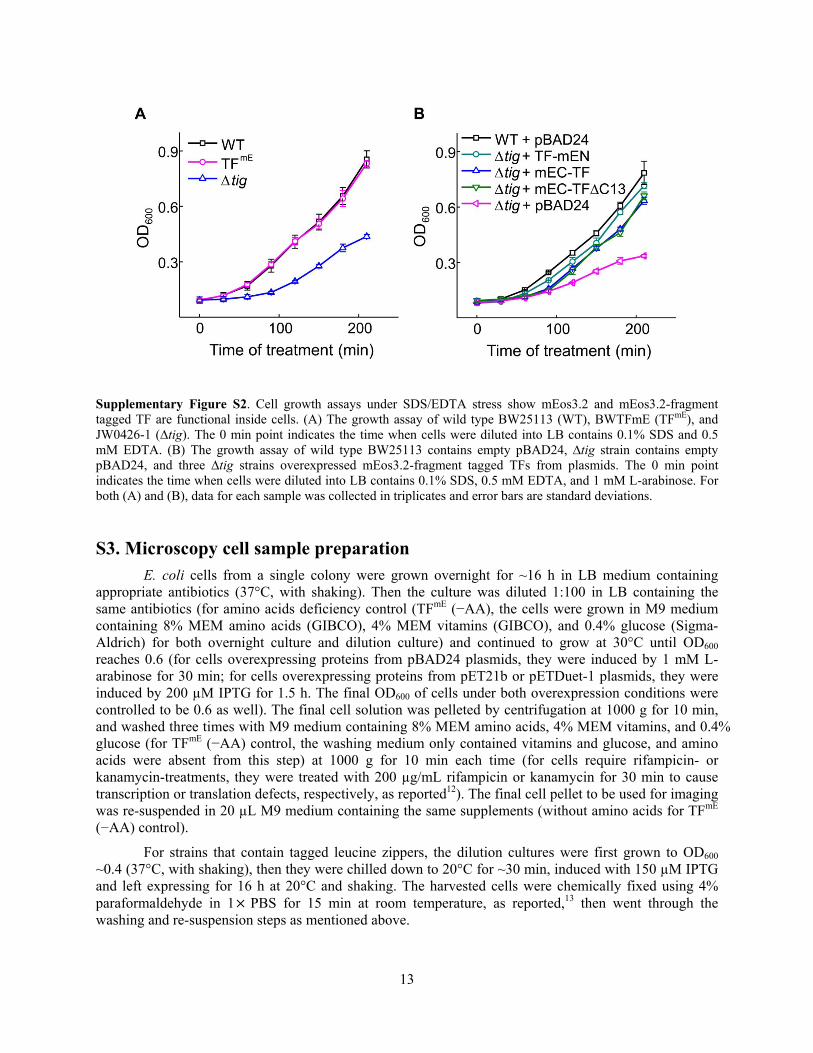
As shown in Supplementary Figure S2A, cells with chromosomal TF tagged with mEos3.2 (TFmE) show identical growth behavior under SDS/EDTA stress to the wild type BW25113 (WT), whereas the ∆tig strain shows much worse growth. These results support mEos3.2-tagged TF is as functional as the untagged TF.

Similarly, as shown in Supplementary Figure S2B, when mEos3.2-fragment tagged TF (TF-mEN, mEC-TF, or mEC-TF∆C13) are expressed from plasmids under induction of L-arabinose, all the ∆tig strains show comparable (slightly less) growth behaviors as the wild type BW25113 (with empty pBAD24 plasmids) under SDS/EDTA stress, whereas the ∆tig strain containing only empty pBAD24 plasmids shows significantly worse growth. These results support mEos3.2-fragment tagged TFs are comparably functional to the untagged TF.

13

Supplementary Figure S2. Cell growth assays under SDS/EDTA stress show mEos3.2 and mEos3.2-fragment tagged TF are functional inside cells. (A) The growth assay of wild type BW25113 (WT), BWTFmE (TFmE), and JW0426-1 (∆tig). The 0 min point indicates the time when cells were diluted into LB contains 0.1% SDS and 0.5 mM EDTA. (B) The growth assay of wild type BW25113 contains empty pBAD24, ∆tig strain contains empty pBAD24, and three ∆tig strains overexpressed mEos3.2-fragment tagged TFs from plasmids. The 0 min point indicates the time when cells were diluted into LB contains 0.1% SDS, 0.5 mM EDTA, and 1 mM L-arabinose. For both (A) and (B), data for each sample was collected in triplicates and error bars are standard deviations.

S3. Microscopy cell sample preparation E. coli cells from a single colony were grown overnight for ~16 h in LB medium containing

appropriate antibiotics (37°C, with shaking). Then the culture was diluted 1:100 in LB containing the same antibiotics (for amino acids deficiency control (TFmE (−AA), the cells were grown in M9 medium containing 8% MEM amino acids (GIBCO), 4% MEM vitamins (GIBCO), and 0.4% glucose (Sigma-Aldrich) for both overnight culture and dilution culture) and continued to grow at 30°C until OD600 reaches 0.6 (for cells overexpressing proteins from pBAD24 plasmids, they were induced by 1 mM L-arabinose for 30 min; for cells overexpressing proteins from pET21b or pETDuet-1 plasmids, they were induced by 200 µM IPTG for 1.5 h. The final OD600 of cells under both overexpression conditions were controlled to be 0.6 as well). The final cell solution was pelleted by centrifugation at 1000 g for 10 min, and washed three times with M9 medium containing 8% MEM amino acids, 4% MEM vitamins, and 0.4% glucose (for TFmE (−AA) control, the washing medium only contained vitamins and glucose, and amino acids were absent from this step) at 1000 g for 10 min each time (for cells require rifampicin- or kanamycin-treatments, they were treated with 200 µg/mL rifampicin or kanamycin for 30 min to cause transcription or translation defects, respectively, as reported12). The final cell pellet to be used for imaging was re-suspended in 20 µL M9 medium containing the same supplements (without amino acids for TFmE (−AA) control).

For strains that contain tagged leucine zippers, the dilution cultures were first grown to OD600

~0.4 (37°C, with shaking), then they were chilled down to 20°C for ~30 min, induced with 150 µM IPTG and left expressing for 16 h at 20°C and shaking. The harvested cells were chemically fixed using 4% paraformaldehyde in 1× PBS for 15 min at room temperature, as reported,13 then went through the washing and re-suspension steps as mentioned above.

14

To make the imaging sample, 30 µL of 100 nm gold nanoparticles (Ted Pella, Inc., Cat. #: 15708-9, used as position markers for drift correction) in 1:1 water-ethanol solution was first drop-casted onto a clean coverslip and allowed to dry at room temperature for ~30 min. 30 µL 3% heat-dissolved agarose in M9 medium containing appropriate supplements were added onto a clean quartz slide with parafilm spacers secured along the sides of the slide. Then another quartz slide was immediately pressed against the liquid agarose until it solidified to become a gel pad. The final cell sample (2 µL) was added on top of this gel pad and then the coverslip with gold nanoparticles was pressed against the pad, spreading and immobilizing the cells on the gel pad. The edges between coverslip and glass slide were sealed with double-sided tape and epoxy to prevent gel drying, as showed in Supplementary Figure S3.

Supplementary Figure S3. Assembly of the sample for imaging. E. coli cells were immobilized on 3% agarose gel pad. The gel pad was sandwiched between a coverslip and a glass slide, sealed by double-sided tape and epoxy.

S4. Imaging setup for single-molecule tracking (SMT) via time-lapse stroboscopic imaging and for single-cell quantification of protein concentration (SCQPC) in living cells

S4.1 Microscope configuration

The imaging was performed on an Olympus IX71 inverted microscope equipped with transmission imaging optics and an electron-multiplying CCD camera (Andor Technology, DU-897E-CSO-#BV, pixel size 16×16 µm2), similar to what was done previously.1 A 60×TIRF oil immersion objective (Olympus PlanApo N 60×oil 1.45) together with a 1.6× magnification changer and a 1.2× C-mount adapter (Spot Diagnostic Instruments, DD12BXC) collectively magnify the image 115.2×. The final image pixel size is 135.4 nm, calibrated by using a high precision Ronchi Ruling (Edmund Optics, 40 line-pairs/mm).

Supplementary Figure S4 shows a schematic diagram of our microscope setup. In the excitation path, an acousto-optic tunable filter (AOTF) (AA, AOTFnC-400.650-TN) was used to shutter 405 nm (CrystaLaser, DL405-100), 488 nm (CrystaLaser, DL488-050) and 561 nm lasers (Coherent, Sapphire 561-200CW). Three laser beams were spatially overlapped using dichroic filters (Chroma, T510lpxrxt and T4251lpxr) and passed a quarter waveplate to change the polarizations to be circularly polarized. All laser lights were then expanded 4 times by an achromatic lens pair and focused (40 cm focus length lens) at the back focal plane of the objective before being reflected toward the objective by a three-band dichroic filter (Chroma, Z408/488/561 rpc) inside the Olympus filter cube. The cells were then excited via epi-illumination with objective-collimated lasers whose beam size at the sample plane is 26 µm (FWHM). The epi-illumination was inclined approximately to be 60 degree from the optical axis of objective to ensure the illumination is through the cell and to decrease background from the medium above. In the detection path, the emission from mEos3.2 passed through the three-band dichroic filter and the green (Chroma, ET525/50 M) or red band-pass filter (Semrock, FF01-617/73) before entering the EMCCD. A 220×220 pixel region of the EMCCD was used during data acquisition. The synchronization

15

between camera and AOTF was through the Precision Control Unit (Andor Technology, ER_PCUT_101, PU-0614) and the imaging protocol was controlled via the Andor iQ 2.6 software. All imaging experiments were conducted at room temperature (~20°C).

Supplementary Figure S4. Schematic diagram of the microscope setup. An AOTF was synchronized with EMCCD camera and shuttered lasers to generate short laser pulses for single-molecule stroboscopic imaging and single-cell quantification of protein concentration. The 405 nm laser was used to photoconvert mEos3.2 from green to red fluorescence form; and the 561 nm laser was used to probe and track red mEos3.2. The 488 nm laser can be used to detect green-fluorescent form of mEos3.2. Figure adopted from reference.1

S4.2 Single-molecule tracking (SMT) via time-lapse stroboscopic imaging

mEos3.2 was photoconverted by 405 nm laser with a power density of 1-10 W/cm2 to ensure less than one mEos3.2 per cell was photoconverted on average. After photoconverting a single mEos3.2 molecule, the camera-synchronized 561 nm laser was shuttered by the AOTF and created pulse trains with short pulse width (Tint) and time lapse (Ttl) to probe and track the photoconverted molecule with power density of 21.7 kW/cm2. The short duration of the 561 nm laser pulse is crucial for obtaining distinct fluorescent point spread function (PSF) from fast moving proteins in each imaging frame. We used Tint = 4 ms for all the experiments, which is similar to the reported Tint =5 ms for tracking single RelA-Dendra2 molecules14 and Tint =4 ms for tracking mEos3.2-tagged transcription regulators.1 For the time lapse, it has to be long enough to sample the residence times but not too long to skip residence times.

16

We found Ttl=60 ms to be optimal by comparing results ranging from 15 to 180 ms. This value is also the same as what was used for tracking mEos3.2-tagged transcription regulator molecules.1

We then used a two-dimensional Gaussian function to fit the fluorescence PSF in each image to obtain the center location of one molecule in the image. This center location represents the average center localization of the molecule within Tint. Combining the center locations of the molecule in all image frames across a time series, a position trajectory was generated. Experimentally, as showed in Supplementary Figure S5, the procedures described above were performed by an imaging cycle that included a photoconversion of a mEos3.2 tagged protein with 405 nm laser for 20 ms (long enough to convert mEos3.2 but not too long to convert multiple molecules) and subsequent 30 snapshots with camera synchronized 561 nm laser with Tint = 4 ms and Ttl = 60 ms. The number of imaging snapshots in each cycle was sufficient to eventually photobleach the mEos3.2 molecule, before the next photoconversion/imaging cycle, which was repeated for 500 times for each cell to collect enough trajectories.

S4.3 Single-cell quantification of protein concentration (SCQPC)

The photoconversion/imaging cycles discussed in S4.2 simultaneously allow us to determine the average fluorescence intensity (i.e.,⟨ ⟩ ) of a single mEos3.2 molecule in each image and the number of mEos3.2 proteins tracked ( ). After 500 photoconversion/imaging cycles, we photoconverted all the remaining green mEos3.2 proteins to their red forms with the 405 nm laser, then we measured the total red fluorescence intensity of the cell using the same 561 nm laser imaging conditions as done in SMT step. Since the average fluorescence intensity ⟨ ⟩ of mEos3.2 molecules for each cell was determined from the same cell, it can be directly used to compare with the total red fluorescence intensity of the cell to calculate the copy number of the remaining proteins.

The schematic of this assay can be found in Supplementary Figure S5. After 500 cycles of SMT, the cells were illuminated with 405 nm laser at 10 W/cm2 for 1 min to convert the rest of the mEos3.2 proteins to red forms followed by 561 nm laser imaging for 2000 frames at the same laser power density and laser exposure time as done in the SMT step. This SCQPC process was repeated for 3 times until all the proteins inside the cell were photoconverted and subsequently photobleached. We then recorded the total red fluorescence intensity of the cell ( = ∑ ; (i=1, 2, 3) is the fluorescence intensity of each SCQPC cycle). Dividing the total fluorescence intensity by the average intensity of a single mEos3.2, ⟨ ⟩⁄ , we obtained the copy number of mEos3.2 tagged proteins in the SCQPC step ( ). Then the total copy number of protein of interest in each cell would be calculated by = ( +) . Here = 41 is a detection efficiency correction factor that accounts for the fact that not 100% mEos3.2 molecules can be photoconverted and detected. We obtained this factor by comparing the average copy number measured from our imaging experiment of many cells and the copy number calculated from SDS-PAGE and Western blot analysis (S2.1), and this detection efficiency is close to the reported value for mEos3.2 under similar imaging condition in which mEos3.2 was also highly expressed (i.e., tens of thousands of copies in each cell).15

To convert the single-cell protein copy number to the cellular protein concentration, we determined the cell volume from its transmission image. The cell boundary in the transmission image was fitted by the model of the cylinder with two hemispherical caps to get the quantitative information on the cell geometry.1,16 The width and length of the cell were defined as 2R and 2R+L (R is the radius of the hemispherical cap, and L is the height of the cylinder) and the volume of the cell was then calculated as (4 3⁄ + ). Then the cellular protein concentration would be ⁄ .

In order to compare cells under different conditions (e.g., DnaK/J knockout, drug treatment, overexpression of SRP, different growth medium, etc.), we used the SCQPC to sort cells into groups with various levels of cellular protein concentration and only compare cells with similar protein concentration

17

level. In this way, our diffusion and residence time analyses can avoid the complication of possible influences of cellular protein concentrations on comparison results.

Supplementary Figure S5. Single-molecule tracking (SMT) with time-lapse stroboscopic imaging and single-cell quantification of protein concentration (SCQPC). For SMT, one (or none) mEos3.2 molecule was photoconverted to its red form during each 20 ms 405 nm laser pulse, then it was probed by 30 imaging snapshots with EMCCD-synchronized 561 nm laser pulses (pulse time Tint = 4 ms, time lapse Ttl = 60 ms). This imaging cycle was repeated for 500 times for each cell. For the SCQPC, the remaining mEos3.2 molecules after the SMT step were photoconverted to the red forms by 405 nm laser illumination for 1 min, and then these molecules were imaged by 561 nm laser for 2000 frames at the same laser power density and laser exposure time as done in the SMT step. This imaging cycle was repeated for 3 times for each cell. Figure adopted from reference.1

S4.4 PALM imaging of fixed cells (strains containing leucine zipper constructs)

For leucine zipper constructs in fixed E. coli cells, we used a continuous activation and imaging mode in which both the 405 nm and the 561 nm lasers illuminated simultaneously, while the EMCCD was operating at a frame rate of 50 ms. This process lasted for one minute for each cell and these accumulated molecular localizations over time allowed for reconstruction of sub-diffraction-limited images.

S5. Single-molecule localization and tracking data analysis

S5.1 Determination of single-molecule locations

Fluorescent images from our SMT experiments were analyzed using home written Matlab (R2012a, Math Works) program iQPALM1 to obtain locations of individual mEos3.2-tagged TF molecules.

18

First, we used the bright filed transmission images to map the cell boundaries by locating pixels around the cell that have the largest intensity contrast. Then the cell boundaries were superimposed onto the corresponding fluorescence image, the area inside boundary was defined as the region of interest (ROI) of each cell.

Second, each original fluorescence image was convolved with a low-pass Gaussian kernel (13×13, σ = 1 pixel) to remove unreasonably small spots to generate a slightly smoothed image. This image is then applied by a boxcar kernel (15×15, pixel value = 1/225) to obtain the non-uniform background image. Subtracting this background image from the previous slightly-smoothed image generates a final image for spot localization.1,17-19 Pixels with intensities above a threshold (the mean value plus 4 standard deviation of the whole image) inside the ROI of the final image were chosen and fitted with a 2D Gaussian function to obtain the information about the center position, intensity, spot size, and localization errors of each detected fluorescent molecule. The fitting function is given below:

( , ) = exp − ( − )2 − ( − )2 +

( , ) is the EMCCD fluorescence intensity counts at the position ( , ). , , ( , ), and ( , ) are the amplitude, background, centroid location, and standard deviation of the Gaussian function fit, respectively. The total EMCCD counts of the fitted spot (cts, the volume under the fitted 2D Gaussian function) is then converted to the total number of fluorescence photons (N) via the equation below, provided by Andor Technology:

= ( ⁄ ) × ( ⁄ ) × 3.65

Here g, S, and QE are the EM gain, sensitivity (electrons per count), and quantum yield of the EMCCD camera in the spectral range of detected fluorescence respectively. The 3.65 is a physical constant for electron creation in silicon (eV per electron) and (in eV) is the energy of a single detected fluorescence photon (chosen at wavelength 580 nm, the peak of mEos3.2 red fluorescence spectrum).

The localization error ( , i = x or y) of the centroid location was estimated according to20,21:

= + 12 + 8

and N are the standard deviation of the 2D Gaussian fit and the total number of photons as described earlier; a is the pixel size; b is the standard deviation of the background.

After the determination of the centroid locations, these locations were corrected for sample drifting using the 100 nm Au nanoparticle markers in the same frame. The drift was calculated via the relative positions of Au nanoparticles to their positions in the first frame. These drift-corrected spots were then filtered based on and . Both too small (i.e., too narrow for a reasonable single-molecule fluorescence PSF) and too big (too wide for a clean PSF image) ones were rejected. The final threshold used was 80 < < 350 nm (i = x and y), same as in our previous study.1

1

2

3

19

S5.2 Generation of SMT trajectories

The final localizations from S5.1 were grouped according to the imaging cycle (30 frames per cycle) to generate the single-molecule tracking trajectories (location vs. time) and the corresponding displacement trajectories (displacement length r per time lapse vs. time). Typically only one or zero mEos3.2 molecules were converted in each photoconversion/imaging cycle. Cycles containing more than one spot in a single frame were removed from further diffusion and residence time analyses due to the difficulty in differentiating positions belonging to different trajectories.

S6. Determination of the number of diffusion states as well as their diffusion constants and fractional populations

S6.1 Probability density function (PDF) and cumulative distribution function (CDF) of displacement length r per time lapse

If a protein diffuses following Brownian diffusion, we can use the well-known equation (in 2D)22 to describe its motion:

( , ) = ∇ ( , )

Here ( , )is the probability distribution function of the displacement vector , ( , )d represents the probability that a single protein is detected within the region [ , + d ] at the time t. D is the diffusion constant, and ∇ is the 2D Laplacian operator. The solution to the above equation is:

( , ) = 14 exp −4

The probability distribution function of the scalar displacement length r, PDF(r, t), in which all angular

space in 2D is included, satisfies PDF( , )d = ( , ) d . Substituting d = d d and = gives:

PDF( , ) = 2 exp −4

Theoretically, fitting the histogram of displacement length r with the equation above will give the corresponding diffusion constant D. However, the choice of bin size in generating the histogram of r is not trivial because the bin size itself may affect the fitting results. To overcome this issue, we turned to use the cumulative distribution function (CDF) of displacement length r. This CDF is obtained by integrating PDF(r, t):

CDF( , ) = PDF( , )d = 1 − exp −4

4

5

6

7

20

To determine the number of diffusion states, corresponding diffusion constants and fractional populations, a linear combination of two or more CDFs of the displacement length r was used as in previous studies.1,14,22-27 This linear combination approach assumes that the interconversion kinetics among the different diffusion states is slower than the experimental time resolution. The validation of this assumption is discussed in S7.3.2. We only used the first displacement of each single-molecule displacement trajectory to avoid the bias toward molecules that have long trajectories so that all molecules contribute equally to the final CDF. The form of CDF fitting function with two (i.e., C2(r)) and three diffusion states ((i.e., C3(r))) are shown below, respectively:

( ) = 1 − exp −4 + 1 − exp −4

( ) = 1 − exp −4 + 1 − exp −4 + 1 − exp −4

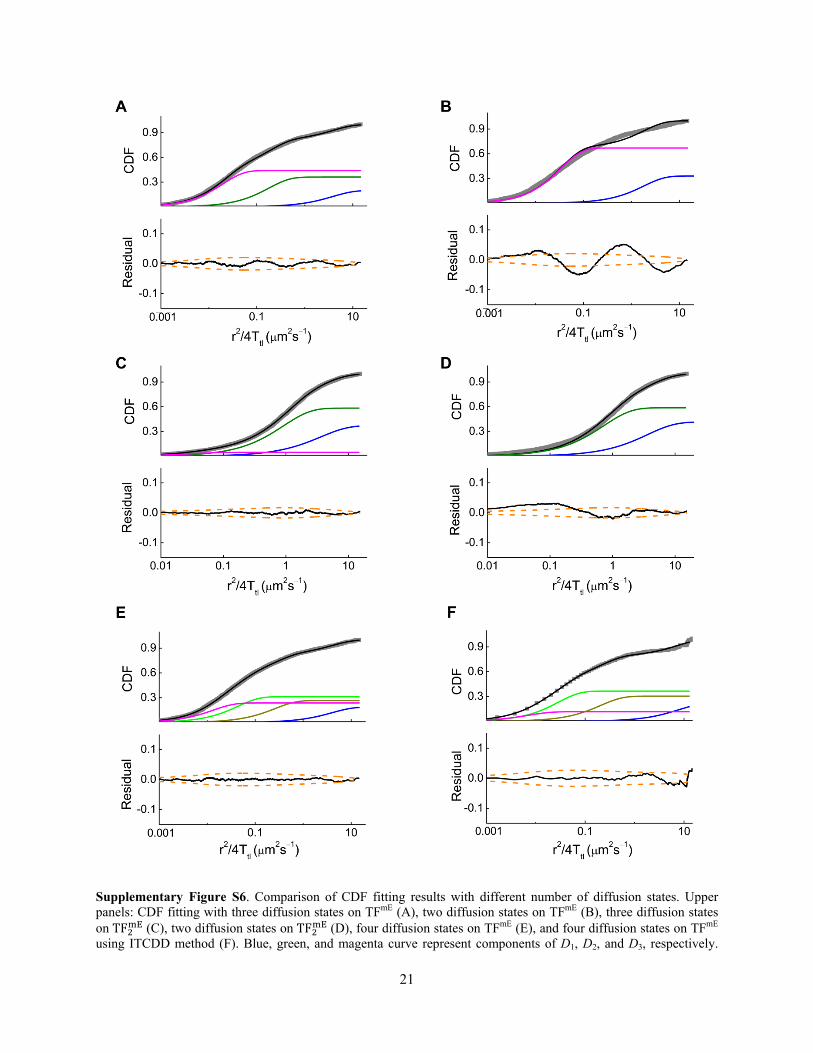
Here , , and are relative amplitudes of different diffusion states (for ( ), + = 1; for ( ), + + = 1) and they represent their fractional populations. , , and are effective diffusion constants. Supplementary Figure S6 shows examples of comparing CDF fitting results with different numbers of diffusion states on TFmE and TF and the corresponding residual analyses. Clearly for TFmE, the fitting quality of CDF with three states is much better than that with two states (Supplementary Figure S6A and B), so the minimal number of diffusion states for this strain is three. And the fitting residuals of CDF with four states (see Section S6.3) are much smaller than the 95% confidence bounds of the data (Supplementary Figure S6E and F), indicating the 4-state model is over-fitting the data. Therefore the 3-state model is sufficient to describe the diffusion of TFmE. For TF , the fitting qualities between 2- or 3-state model do not show much difference (Supplementary Figure S6C and D), and even if fitted with three states the fractional population of D3 is negligible (< 5%), thus the minimal number of diffusion states for this strain is two.

Supplementary Table S4 summaries the CDF fitting results of constructs we studied.

8

9

21

Supplementary Figure S6. Comparison of CDF fitting results with different number of diffusion states. Upper panels: CDF fitting with three diffusion states on TFmE (A), two diffusion states on TFmE (B), three diffusion states on TF (C), two diffusion states on TF (D), four diffusion states on TFmE (E), and four diffusion states on TFmE using ITCDD method (F). Blue, green, and magenta curve represent components of D1, D2, and D3, respectively.

22

Additional colored curves in (E) and (F) represent component of D4. Black curve is the overall fitted function. Lower panels: residuals of the CDF fitting from the upper panels. Orange dashed lines are the 95% confidence interval and the black lines are the residuals.

Supplementary Table S4. Effective diffusion constants and fractional populations from CDF analysis

D1 (µm2s–1) D2 (µm2s–1) D3 (µm2s–1) A1 (%) A2 (%) A3 (%)

# of

trajectories

Average trajectory

length (# of positions) TF 3.85 ± 0.14 0.18 ± 0.04 0.02 ± 0.01 20 ± 2 36 ± 3 44 ± 1 6934 3.10 ± 2.42 TF (p) 3.84 ± 0.24 0.72 ± 0.08 0.05 ± 0.01 31 ± 2 52 ± 1 16 ± 1 11448 3.05 ± 2.02 TF / (p) 3.76 ± 0.15 0.92 ± 0.07 0.04 ± 0.01 37 ± 1 58 ± 2 5 ± 1 5420 2.81 ± 1.58 TF + Rif 3.87 ± 0.10 0.42 ± 0.06 0.04 ± 0.02 28 ± 3 59 ± 1 12 ± 3 10400 2.84 ± 1.66 TF + Kan 3.74 ± 0.07 0.36 ± 0.02 0.06 ± 0.02 25 ± 4 49 ± 3 26 ± 4 9916 2.94 ± 1.74 TF∆ 3.52 ± 0.10 0.28 ± 0.02 0.04 ± 0.01 16 ± 3 54 ± 2 29 ± 4 6124 3.16 ± 1.98 TF∆ 3.68 ± 0.14 0.28 ± 0.01 0.04 ± 0.01 17 ± 2 50 ± 5 33 ± 4 5299 3.01 ± 1.89 TF (–AA) 3.56 ± 0.22 0.50 ± 0.09 0.05 ± 0.01 29 ± 2 54 ± 2 17 ± 2 8289 2.76 ± 1.38 TF + SRP 3.78 ± 0.13 0.20 ± 0.03 0.04 ± 0.01 16 ± 4 48 ± 2 36 ± 3 5511 3.00 ± 1.84 TF 3.04 ± 0.10 0.62 ± 0.06 51 ± 2 49 ± 1 8888 2.81 ± 1.58 TF (p) BL21a 3.96 ± 0.27 0.42 ± 0.06 0.04 ± 0.01 20 ± 1 58 ± 2 22 ± 2 7800 2.78 ± 1.54 TF ,∆ 3.75 ± 0.15 0.94 ± 0.10 0.02 ± 0.01 32 ± 1 58 ± 2 10 ± 2 4590 2.96 ± 1.90 TF + Kan 3.09 ± 0.14 0.55 ± 0.04 64 ± 3 36 ± 2 6052 2.91 ± 1.68

a All the TF dimer constructs and ones labeled “BL21” are in BL-21(DE3); while other constructs are in BW25113 strain.

S6.2 Validation of diffusion state analysis using hidden Markov model

In addition to the CDF analysis, we further performed hidden Markov model analysis using the vbSPT (variational Bayes Single Particle Tracking) software28 to extract diffusion states from our SMT data.

In this analysis, trajectories with minimally 2 positions (1 displacement) were used as inputs, while the dimensionality of the displacement is 2 (along both x and y directions). For the data with minimally three diffusion states from CDF analysis, we initially allowed maximally N = 6 states in the vbSPT software, the output gave the optimal number of diffusion states as N = 3, 4, 5, or 6, with similar model scores (the differences compared to the highest model score (dF) are ~−100 to 0, the closer to zero the better), better than N = 1 or 2 (dF = −Inf to ~−2000). So the minimal number of diffusion states is still three. For the data with minimally two diffusion states from CDF analysis, the same conclusion was also obtained from vbSPT analysis. Example outputs for TFmE and TF are shown in Supplementary Figure S7. The details of comparison between vbSPT results and CDF results are shown in Supplementary Table S5. All the diffusion constants (D1, D2, and D3) are very similar while the fractional populations of relatively slow-moving molecules obtained from vbSPT analysis are slightly larger.

23

Supplementary Figure S7. Hidden Markov model analysis via vbSPT. Example outputs of hidden Markov model analysis using vbSPT software on TFmE (A) and TF (B). Blue, green, and magenta circles represent diffusion states of D1, D2, and D3, respectively. The area of the circle indicates the fractional population while the thickness of arrow line indicates the transition probability.

S6.3 Validation of diffusion state analysis using inverse transformation of the confined displacement distribution (ITCDD) method

Furthermore, we applied the ITCDD method29 to validate our diffusion analysis, as we developed in a previous paper29. Due to the cell confinement effect, the displacement length distribution of proteins is distorted29,30. Thus we used ITCDD method to convert the distorted displacement length distribution back to that in free space to resolve the intrinsic diffusion constants and corresponding fractional populations. We first obtained the average cell geometry parameters (length and width) as mentioned in S4.3 and performed simulations to build the confinement transformation matrix (i.e., [CTM]) for each set of data. Then the PDF of displacement length r in free space (i.e., PDFFS) can be obtained by performing inverse transformation on PDF of displacement length r in confined space in the cell (i.e., PDFCS):PDF = CTM ∙ PDF , as described in our previous study.29 Finally the corresponding CDF of displacement length r in free space (i.e., CDFFS) was generated. The final results were compared with those from regular CDF analysis (Supplementary Table S5). The intrinsic diffusion constant of free diffusing state (D1) is much larger from ITCDD method than the effective diffusion constant in CDF analysis because the fast moving molecules are affected most by the cell confinement effect.29 Other diffusion constants and all the fractional populations are very similar between these two methods.

Supplementary Table S5. Comparison of fitting results using different methods.

TF TF Method CDF vbSPT ITCDDa CDF vbSPT ITCDDa

D1 (µm2s–1) 3.85 ± 0.14 4.40 ± 0.42 7.3 ± 2.4 3.04 ± 0.10 3.91 ± 0.47 6.3 ± 1.5 D2 (µm2s–1) 0.18 ± 0.04 0.19 ± 0.05 0.20 ± 0.02 0.62 ± 0.06 0.78 ± 0.17 0.86 ± 0.13 D3 (µm2s–1) 0.02 ± 0.01 0.02 ± 0.01 0.02 ± 0.01

A1 (%) 20 ± 2 14 ± 1 21 ± 1 51 ± 2 32 ± 2 50 ± 4 A2 (%) 36 ± 3 31 ± 3 33 ± 3 49 ± 1 68 ± 4 50 ± 3 A3 (%) 44 ± 1 54 ± 4 45 ± 2

a Note the diffusion constants from ITCDD, where the cell confinement effect is accounted for, are intrinsic diffusion constants, whereas those from CDF and vbSPT analysis are effective diffusion constants that are affected by cell geometry and imaging time resolution.

24

S7. Determination of unbinding kinetics of TF from the 70S ribosome The SMT trajectories (location vs. time) gave the corresponding displacement trajectories

(displacement length r vs. time), as discussed in S5.2. When TF binds to the 70S ribosome, its movement becomes very slow (almost stationary) and the corresponding displacement length per time lapse will be very small. Therefore, we can define an upper threshold of displacement length (220 nm, below which >99% displacement lengths and the corresponding positions of the 70S-ribosome-bound state (D3 state) are included; Figure 2C in the main text) to identify the microscopic residence time of TF molecules bound on the 70S ribosome (Figure 5A in the main text).

S7.1 Determination of photobleaching/blinking kinetics of mEos3.2 in E. coli cells

Because of the photobleaching/blinking behaviors of mEos3.2, the measured residence time will end not only due to the unbinding of TF from the 70S ribosome but also due to photophysical properties of the mEos3.2 tag, and thus we need a correction for this measurement.

We used the emission intensity vs. time trajectory (which shows on-off photoblinking behaviors and eventually becomes permanently dark from photobleaching, as shown in Supplementary Figure S8A) to extract the distribution of emission on time (i.e., ). This distribution can give us the photobleaching/blinking rate constant, , which is the sum of bleaching and blinking rate constants. However, unlike the photophysical studies with continuous imaging scheme,31,32 we used stroboscopic imaging in which our excitation laser pulse is only on for , which is just a portion of total time-lapse . So the apparent photobleaching/blinking rate constant will equal to the intrinsic under continuous illumination condition corrected by a factor ⁄ to account for the time-lapse imaging effect. Therefore, the distribution of can be fitted by the equation below:

( ) = exp −

Here C is a normalization constant. An example of fitting is shown in Supplementary Figure S8B. The extracted from this fitting is 248 ± 13 s−1, which is closed to the reported value (257 ± 9 s−1) under similar imaging conditions.1

Supplementary Figure S8. Photobleaching/blinking kinetics of mEos3.2. (A) An example of single-molecule emission intensity vs. time trajectory of TFmE in one imaging cycle. The fluorescence intensities below the threshold

10

25

(the mean value plus four standard deviation of the whole image) are represented by zero. (B) The distribution of for TFmE (black dots) and the fitting using Equation 10 (magenta curve), giving kbl = 248 ± 13 s−1.

S7.2 Determination of the photobleaching/blinking corrected unbinding rate constant of TF from the 70S ribosome

After obtained the photobleaching/blinking constant , we can fit the distribution of residence time with a single exponential function shown below:

= exp − +

Here C is the normalization constant. is the apparent unbinding rate constant of TF from the 70S ribosome.

S7.3 Validation of the unbinding kinetics analysis via changing the threshold r0 and hidden Markov model analysis

After thresholding by the upper limit , the small displacements are dominated by TF in the D3 state (70S-ribosome-bound state); yet there is some contribution from TF in the D2 state as well (about 35% for TFmE). And the amount of this contribution varies across different strains used in this study due to different fractional populations of D3 and D2 states. Therefore the values of the unbinding rate constant determined could change with different thresholds. To probe whether this issue affects the conclusions drawn from the kinetics analysis, we used two approaches for validation.

S7.3.1 Varying r0 to make the integrated area ratio between D2 and D3 population below the threshold in PDF be the same and repeat the kinetics analysis

Instead of fixing a single threshold for all strains used in this study. We varied for each strain to make the integrated area ratio between D2 and D3 populations below the r0 threshold in PDF be the same as that for the TFmE strain (i.e., our base strain for comparison) so that the contribution of TF in the D2 state would be the same in the thresholded displacements across all the conditions. The results are shown in Supplementary Figure S9, all the trends are consistent with the original analysis using fixed = 220 nm:

• The unbinding rate constant of TFmE (−AA) (amino acids deficiency control) or TFmE with Kan treatment is significantly larger than that of TFmE under normal conditions (Supplementary Figure S9A, B).

• The unbinding rate constant of TF∆ (DnaK knockout control) or TF∆ (DnaJ knockout control) does not show clear difference compared with that of TFmE (Supplementary Figure S9C).

• Overexpression of SRP does not change the unbinding rate constant of TFmE significantly (Supplementary Figure S9D).

S7.3.2 Validation of the kinetics analysis using hidden Markov model

The vbSPT software28 is based on hidden Markov model analysis and does not require thresholding, thus we extracted the unbinding rate constants directly using this software and confirmed all the trends are, again, consistent with the original kinetics analysis. The absolute values of the unbinding

11

26

rate constant determined here are different from those obtained from our r0 thresholding method, possibly due to the inevitable contributions of TFmE in the D2 state to the thresholded displacement lengths r. The results are also shown in Supplementary Figure S9. Compared with TFmE under normal conditions, the unbinding rate constants of TFmE (−AA) and TFmE with Kan treatment show clear increases (Supplementary Figure S9A, B), whereas the unbinding rate constants of TF∆ , TF∆ , and TFmE with overexpression of SRP do not change significantly (Supplementary Figure S9C, D).

The vbSPT also gives the average lifetimes of D1, D2, and D3 states of TFmE to be ~0.19 s, ~0.50 s, and ~1.4 s, all are significantly longer than our experimental time resolution 60 ms, which supports that the interconversions among different diffusion states are slow enough to ensure the linear combination of CDFs in our diffusion analysis (S6.1) be valid.

Supplementary Figure S9. Our conclusions about the unbinding rate constants of TFmE from 70S ribosome from kinetics analysis are independent of the choice of r0 as well as of using three different methods.

S8. Spatial distribution analysis of TF in living cells

S8.1 Uncovering the clustering of TFs using the probability distribution of pairwise distances

S8.1.1 General procedures of pairwise distance analysis

27

In order to quantify the heterogeneity of the spatial distribution of TFs in living cells, we calculated pairwise distances between first positions (to avoid the bias toward long trajectories) of all tracking trajectories in each cell. By combining results from many cells, we could obtain the probability distribution of pairwise distances of specific strains. In addition, we also applied the r0 threshold (see Section S7) to divide positions into a subgroup corresponding to TF molecules bound to the 70S ribosome (D3 state positions) and the other subgroup of the rest positions.

To quantify the degree of heterogeneity of the probability distribution of pairwise distances, we performed a simulation to generate a uniform distribution of positions within the cell, as a reference. First, we divided cells from a specific experiment into four groups according to their geometric size (from small to large, the determination of cell geometric size is described in S4.3). For each group of cells, we calculated the average cell length and width, the number of cells, and the average number of first positions (i.e., the average number of tracking trajectories) per cell. Second, we simulated four corresponding groups of cells, each group containing the same number of cells as the corresponding experimental group, and each cell within the same group having the cell length and width, and the number of first positions, same as the average values from the corresponding experimental group as well. However, the spatial distribution of simulated positions in the cells is uniform so that there are no spatial patterns. The simulation of uniform distribution is done by randomly placing positions (same number as the average number of first positions in each group) within the cell boundary (with length and width same as the average values in each group). Finally, we obtained the probability distribution of pairwise distances from our simulated cells as mentioned above.

By subtracting the probability distribution of pairwise distances of simulated cells from our experimental results (both experimental and simulated probability distribution have the same bin size), we can use the difference to estimate the degree of spatial heterogeneity and identify potential clustering of TF positions within the cells. Peaks appearing in the difference of probability distribution at short pairwise distances would indicate clustering of TFs in the cell and we can use the peak positions to estimate the cluster sizes. However, since our imaging was always done on living cells, the locations of clusters may change due to motions during the sampling of positions of molecules, which would diminish the observed clustering effect in the pairwise distance distributions. Therefore, the cluster size determined from the pair-wise distance distribution analysis here should reflect an upper limit of the real cluster size.

S8.1.2 Pairwise distance analyses of TFmEFRK/AAA and TF2

mE do not show the existence of clusters; whereas the analysis of TF2,ΔC13

mE does

Supplementary Figure S10A and B show the probability difference of pairwise distance distribution of TF / and TF compared with the simulation results of uniform position distributions in the cell, respectively.

No significant peaks (indicating the existence of clusters) can be found within short distances (i.e., <100 nm) in either of them, which supports that neither of these strains contains a 70S-ribosome-bound TF population (i.e., D3 state).

Supplementary Figure S10C shows the probability difference of pairwise distance distribution of TF ,∆ for which we can resolve the D3 state in the CDF analysis (Supplementary Table S4), compared

with its corresponding simulation results of the uniform position distribution. Here the pair-wise distance distribution for the D3 state shows a clear peak at ~60 nm, which is similar to that of TFmE. This result

supports that once the dimerization ability of TF is impaired by the ΔC13 truncation, the complementation complex (two TF monomers linked by a complemented mEos3.2) can regain the capability of binding to the 70S ribosome.

28

Supplementary Figure S10. Pairwise distance distributions between first positions of tracking trajectories. Probability difference of pairwise distance distributions for (A)TF / , (B) TF , and (C) TF ,∆ relative to their corresponding simulated uniform distribution inside cells.

S8.2 Distribution of TF molecule positions along the cell short axis reveals the nucleoid exclusion effect of the 70S ribosome inside the cells

According to previous studies33 , 70S ribosomes are excluded from the nucleoid region of E. coli (the nucleoid usually is located in the middle of the cell), whereas the free ribosomal subunits are homogenously distributed throughout the cell. Thus, by examining the spatial distribution of TFmE positions along the short axis of cells, we should observe lower density in the middle of cells if some TFmE molecules are bound to 70S ribosomes.

In order to do this, we normalized the geometry and overlaid multiple cells (as well as first positions of TF tracking trajectories in them) from each specific experiment condition using the average cell length and width. We also applied the r0 threshold as done in S8.1.1 to divide TF positions into a subgroup corresponding to TF molecules bound to the 70S ribosome (D3 state positions) and the other subgroup of the rest positions. In each subgroup, the 1st positions of TF tracking trajectories in the cylinder region of the normalize cell (i.e., excluding the two hemispherical ends) were projected onto the short axis of the cell to generate the position probability (bin size: one tens of the cell width, ~100 nm). As a control, we performed a simulation that have the same number of positions as the corresponding experimental cells but are uniformly distributed within the cell. Finally, by comparing the probability distribution of positions along the cell short axis between experimental results and the corresponding simulated results, we can uncover the molecular density difference inside the cells.

S8.2.1 Distributions of positions of TFmEFRK/AAA and TF2

mE do not show a decreased probability in the middle of the cell along the cell short axis

Supplementary Figure S11A and B show the distributions of positions of TF / and TF , along the cell short axis, respectively. They do not show less probabilities in the middle region of the cell compared with their corresponding simulated results with a uniform distribution, which supports that neither of these TF variants contains a population that bounds to the 70S ribosome, which would be excluded from the nucleoid region of the cell.

29

Supplementary Figure S11. Distribution of molecular positions along the cell short axis. The distribution of positions of (A) TF / and (B) TF (magenta curves) from overlaid cells compared with the simulated uniform distribution (black dashed curves).

S8.2.2 Quantification of the degree of nucleoid exclusion using the spatial distribution of TFmE positions in the D3 state further supports that the D3 state is the 70S ribosome bound state

To further support that the D3 state of TFmE is the 70S-ribosome-bound population, we performed another simulation in which molecular positions are excluded from a cylinder with varying radius re in the center of the cell (Supplementary Figure S12A, similar as Elf and coworkers did previously33). By comparing the spatial distribution of the TF positions in the D3 state along the cell short axis with this simulation, we can estimate the degree of exclusion of the D3 population form the center of the cell, which, should behave similarly as the exclusion of 70S ribosomes if this population is indeed bound to 70S ribosomes.

Supplementary Figure S12B and C show the results of D3 states of TFmE and TFmE + Kan (i.e., Kan treatment) in comparison with the simulations that have an excluded region in the middle of the cell. Clearly, the exclusion radius re decreases after the Kan treatment, which is consistent with the previous findings that Kan causes nucleoid contraction.12,34-36 This further supports that the D3 state of TFmE is the 70S-ribosome-bound state.

In addition, to validate the exclusion effect in our data (the dent in the middle of probability distribution of molecular positions along the cell short axis), we subtracted the probability distribution of TFmE positions in the D3 state (blue curve, Figure S12B) from the uniform distribution simulation (black dashed curve). The probability difference of the bin corresponding to the bottom of the dent is ~0.027, larger than the mean plus two standard deviations of the probability differences of the rest bins (~0.019), indicating the probability of D3 state positions of TFmE in the middle of the cells is significantly smaller than the probability of uniform distribution in the same area. Therefore, the dent in this probability distribution reflects the actual spatial pattern rather than random noises.

30

Supplementary Figure S12. Estimation of the degree of exclusion from the distribution of positions along the cell short axis. In addition to the uniform distribution simulation (black dashed curves), models of exclusion from the center of a cylinder with radius re (A) were used to compare with the distribution of positions of (B) TFmE and (C) TFmE +Kan (i.e., Kan treatment of TFmE).

S9. Validation and additional information about PC-BiFC

S9.1 Validation of PC-BiFC using leucine zipper system

We first validated our PC-BiFC design using leucine zipper system mEC-NZ and CZ-mEN (Supplementary Figure S13A and B). Once the two leucine zippers NZ and CZ assemble, the two mEos3.2 fragments mEC and mEN can complement and become fluorescent, and we can use PALM to obtain the localizations of the complemented complex. Each of these localizations was then convoluted with a standard 2D Gaussian function (whose FWHM is ~32 nm, which is about the average localization accuracy of individual molecules in PALM imaging) to generate a reconstructed PALM image for each cell. Examples of reconstructed PALM images are shown in Supplementary Figure S13C, D, and E). The spatial distribution of this complemented complex is homogenous inside the cells, as expected.4

We did a further validation using another system mEC-NZ and Tsr-CZ-mEN, in which Tsr is an inner-membrane protein5,6 (Supplementary Figure S14A and B) and it targets the complemented complex to the cell membrane. Supplementary Figure S14C, D, and E show examples of reconstructed PALM images for this system. Clear accumulations of proteins on the membrane were observed, which agrees with the spatial distribution of Tsr.

These results above support that our PC-BiFC method works effectively.

31

Supplementary Figure S13. Schematic diagram of (A) design of CZ-mEN and mEC-NZ constructs and (B) the complementation strategy. Below, (C), (D), and (E) show reconstructed super-resolution PALM images (red images) of selected cells expressing these constructs. Insets show bright-field transmission images (upper corners) and diffraction-limited epi-fluorescence images (lower corners) of the same cells, but resized to 50% of the PALM images.

32

Supplementary Figure S14. Schematic diagram of (A) design of Tsr-CZ-mEN and mEC-NZ constructs and (B) the complementation strategy. Below, (C), (D), and (E) show reconstructed super-resolution PALM images (red images) of selected cells expressing these constructs. Insets show bright-field transmission images (upper corners) and diffraction-limited epi-fluorescence images (lower corners) of the same cells, but resized to 50% of the PALM images.

S9.2 The two TFs in TF2mE dominantly exist in the dimerized form rather than two

monomers tethered by the complemented mEos3.2

Supplementary Figure S15A shows a structural model of TF2mE using linker L1 and L2 between

TF and the two mEos3.2 fragments (see S1.6.2). The structure of the TF2 dimer was based on the reported TF2 dimer from Vibrio cholera (PDB ID: 1T11).37

The irreversible complementation of the two mEos3.2 fragments essentially tethers the two TF monomers, forcing them to stay dominantly as a TF2 dimer because of the increased local effective protein concentration, while minimizing the dissociated two-monomer form. The two linkers between TF and the mEos3.2-fragments, if fully stretched, bring the two TF protein molecules within about rm ~ 5 nm to each other. Relative to one TF, the other TF is essentially confined approximately to a surrounding

spherical space of (Supplementary Figure S15B), leading to an effective local protein

concentration of 1 (⁄ ), which is ~3000 μM. Considering that the natural TF2 dimer has a

dissociation constant Kd of ~2 µM,38 this effective concentration of ~3000 μM will ensure that the complementation-tethered TF2

mE dimer will stay at the dimerized form for >98% of time. Therefore, the PC-BiFC strategy traps TF2

mE into the dimer form, which we could then study using single-molecule tracking measurements.

33

Supplementary Figure S15. (A) Structural model of TF2mE in two orientations (~180° difference). (B) Schematic of

the effective volume of a pair of TFs tethered by a complemented mEos3.2, centered at one TF molecule with a radius of rm.

S9.3 The complementation of mEos3.2 fragments is mainly due to target protein interactions, and the spontaneous fragment complementation is much less significant

Even without any target protein interactions (e.g., TF dimerization), the two mEos3.2 fragments may still encounter and complement (i.e., spontaneous complementation). In order to estimate how much this effect contributes to the overall complementation, we quantified the detected complementation complex concentrations in the cell using the SCQPC approach introduced in S4.3, where we did not use detection efficiency correction factor. We compared TF , the complementation between mEC-TF and TF-mEN, and TF ,∆ , the complementation complex between mEC-TF∆C13 and TF-mEN in which TFΔC13 has reduced capability for dimerization3 so the complementation of mEos3.2 fragments has a significant contribution from the spontaneous complementation. The average cellular concentration of detected complemented complex of TF is more than twice of that of TF ,∆ , (Supplementary Figure S16A vs B), which supports that the specific complementation due to target protein interactions is more efficient than spontaneous complementation of mEos3.2 fragments.

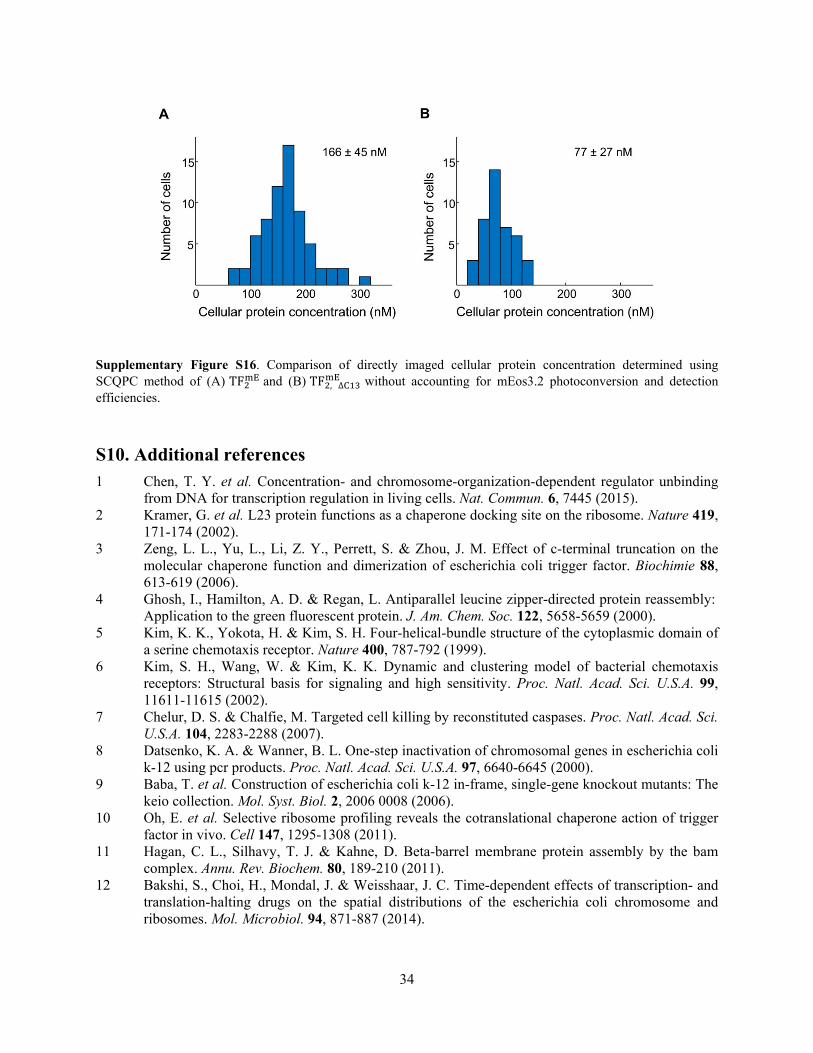
34

Supplementary Figure S16. Comparison of directly imaged cellular protein concentration determined using SCQPC method of (A) TF and (B)TF ,∆ without accounting for mEos3.2 photoconversion and detection efficiencies.

S10. Additional references 1 Chen, T. Y. et al. Concentration- and chromosome-organization-dependent regulator unbinding

from DNA for transcription regulation in living cells. Nat. Commun. 6, 7445 (2015). 2 Kramer, G. et al. L23 protein functions as a chaperone docking site on the ribosome. Nature 419,

171-174 (2002). 3 Zeng, L. L., Yu, L., Li, Z. Y., Perrett, S. & Zhou, J. M. Effect of c-terminal truncation on the

molecular chaperone function and dimerization of escherichia coli trigger factor. Biochimie 88, 613-619 (2006).

4 Ghosh, I., Hamilton, A. D. & Regan, L. Antiparallel leucine zipper-directed protein reassembly:  Application to the green fluorescent protein. J. Am. Chem. Soc. 122, 5658-5659 (2000).

5 Kim, K. K., Yokota, H. & Kim, S. H. Four-helical-bundle structure of the cytoplasmic domain of a serine chemotaxis receptor. Nature 400, 787-792 (1999).

6 Kim, S. H., Wang, W. & Kim, K. K. Dynamic and clustering model of bacterial chemotaxis receptors: Structural basis for signaling and high sensitivity. Proc. Natl. Acad. Sci. U.S.A. 99, 11611-11615 (2002).

7 Chelur, D. S. & Chalfie, M. Targeted cell killing by reconstituted caspases. Proc. Natl. Acad. Sci. U.S.A. 104, 2283-2288 (2007).

8 Datsenko, K. A. & Wanner, B. L. One-step inactivation of chromosomal genes in escherichia coli k-12 using pcr products. Proc. Natl. Acad. Sci. U.S.A. 97, 6640-6645 (2000).

9 Baba, T. et al. Construction of escherichia coli k-12 in-frame, single-gene knockout mutants: The keio collection. Mol. Syst. Biol. 2, 2006 0008 (2006).

10 Oh, E. et al. Selective ribosome profiling reveals the cotranslational chaperone action of trigger factor in vivo. Cell 147, 1295-1308 (2011).

11 Hagan, C. L., Silhavy, T. J. & Kahne, D. Beta-barrel membrane protein assembly by the bam complex. Annu. Rev. Biochem. 80, 189-210 (2011).

12 Bakshi, S., Choi, H., Mondal, J. & Weisshaar, J. C. Time-dependent effects of transcription- and translation-halting drugs on the spatial distributions of the escherichia coli chromosome and ribosomes. Mol. Microbiol. 94, 871-887 (2014).

35

13 Betzig, E. et al. Imaging intracellular fluorescent proteins at nanometer resolution. Science 313, 1642-1645 (2006).

14 English, B. P. et al. Single-molecule investigations of the stringent response machinery in living bacterial cells. Proc. Natl. Acad. Sci. U.S.A. 108, E365-373 (2011).

15 Wang, S., Moffitt, J. R., Dempsey, G. T., Xie, X. S. & Zhuang, X. Characterization and development of photoactivatable fluorescent proteins for single-molecule-based superresolution imaging. Proc. Natl. Acad. Sci. U.S.A. 111, 8452-8457 (2014).

16 Itan, E., Carmon, G., Rabinovitch, A., Fishov, I. & Feingold, M. Shape of nonseptated escherichia coli is asymmetric. Phys. Rev. E. Stat. Nonlin. Soft Matter Phys. 77, 061902 (2008).

17 Henriques, R. et al. Quickpalm: 3d real-time photoactivation nanoscopy image processing in imagej. Nat. Meth. 7, 339-340 (2010).

18 Gould, T. J., Verkhusha, V. V. & Hess, S. T. Imaging biological structures with fluorescence photoactivation localization microscopy. Nat. Protoc. 4, 291-308 (2009).

19 Bakshi, S., Bratton, B. P. & Weisshaar, J. C. Subdiffraction-limit study of kaede diffusion and spatial distribution in live escherichia coli. Biophys J 101, 2535-2544 (2011).

20 Thompson, R. E., Larson, D. R. & Webb, W. W. Precise nanometer localization analysis for individual fluorescent probes. Biophys. J. 82, 2775-2783 (2002).

21 Yildiz, A. et al. Myosin v walks hand-over-hand: Single fluorophore imaging with 1.5-nm localization. Science 300, 2061-2065 (2003).

22 Schutz, G. J., Schindler, H. & Schmidt, T. Single-molecule microscopy on model membranes reveals anomalous diffusion. Biophys. J. 73, 1073-1080 (1997).

23 Gebhardt, J. C. et al. Single-molecule imaging of transcription factor binding to DNA in live mammalian cells. Nat. Meth. 10, 421-426 (2013).

24 Mazza, D., Abernathy, A., Golob, N., Morisaki, T. & McNally, J. G. A benchmark for chromatin binding measurements in live cells. Nucleic Acids Res. 40, e119 (2012).

25 Niu, L. & Yu, J. Investigating intracellular dynamics of ftsz cytoskeleton with photoactivation single-molecule tracking. Biophys. J. 95, 2009-2016 (2008).

26 Uphoff, S., Reyes-Lamothe, R., Garza de Leon, F., Sherratt, D. J. & Kapanidis, A. N. Single-molecule DNA repair in live bacteria. Proc. Natl. Acad. Sci. U.S.A. 110, 8063-8068 (2013).

27 Mueller, F., Stasevich, T. J., Mazza, D. & McNally, J. G. Quantifying transcription factor kinetics: At work or at play? Crit. Rev. Biochem. Mol. Biol. 48, 492-514 (2013).

28 Persson, F., Linden, M., Unoson, C. & Elf, J. Extracting intracellular diffusive states and transition rates from single-molecule tracking data. Nat. Meth. 10, 265-269 (2013).

29 Chen, T. Y. et al. Quantifying multistate cytoplasmic molecular diffusion in bacterial cells via inverse transform of confined displacement distribution. J. Phys. Chem. B. 119, 14451-14459 (2015).

30 Oswald, F., E, L. M. B., Bollen, Y. J. & Peterman, E. J. Imaging and quantification of trans-membrane protein diffusion in living bacteria. Phys. Chem. Chem. Phys. 16, 12625-12634 (2014).

31 Annibale, P., Vanni, S., Scarselli, M., Rothlisberger, U. & Radenovic, A. Quantitative photo activated localization microscopy: Unraveling the effects of photoblinking. PLoS One 6, e22678 (2011).

32 Lee, S. H., Shin, J. Y., Lee, A. & Bustamante, C. Counting single photoactivatable fluorescent molecules by photoactivated localization microscopy (palm). Proc. Natl. Acad. Sci. U.S.A. 109, 17436-17441 (2012).

33 Sanamrad, A. et al. Single-particle tracking reveals that free ribosomal subunits are not excluded from the escherichia coli nucleoid. Proc. Natl. Acad. Sci. U.S.A. 111, 11413-11418 (2014).

34 Misumi, M. & Tanaka, N. Mechanism of inhibition of translocation by kanamycin and viomycin: A comparative study with fusidic acid. Biochem. Biophys. Res. Commun. 92, 647-654 (1980).

35 Pestka, S. The use of inhibitors in studies on protein synthesis. Meth. Enzymol. 30, 261-282 (1974).

36

36 Sohmen, D., Harms, J. M., Schlunzen, F. & Wilson, D. N. Snapshot: Antibiotic inhibition of protein synthesis i. Cell 138, 1248 e1241 (2009).

37 Ludlam, A. V., Moore, B. A. & Xu, Z. The crystal structure of ribosomal chaperone trigger factor from vibrio cholerae. Proc. Natl. Acad. Sci. U.S.A. 101, 13436-13441 (2004).

38 Maier, R., Eckert, B., Scholz, C., Lilie, H. & Schmid, F. X. Interaction of trigger factor with the ribosome. J. Mol. Biol. 326, 585-592 (2003).