Single-Trial Analysis and Classification ofERP Components – a Tutorial

Benjamin Blankertz∗,a,b, Steven Lemmb, Matthias Tredera, Stefan Haufea, Klaus-Robert Müllera

aBerlin Institute of Technology, Machine Learning Laboratory, Berlin, GermanybFraunhofer FIRST, Intelligent Data Analysis Group, Berlin, Germany

Abstract

Analyzing brain states that correspond to event related potentials (ERPs) on a single trial basis isa hard problem due to the high trial-to-trial variability and the unfavorable ratio between signal(ERP) and noise (artifacts and neural background activity). In this tutorial, we provide a compre-hensive framework for decoding ERPs, elaborating on linear concepts, namely spatio-temporalpatterns and filters as well as linear ERP classification. However, the bottleneck of these tech-niques is that they require an accurate covariance matrix estimation in high dimensional sensorspaces which is a highly intricate problem. As a remedy, we propose to use shrinkage estima-tors and show that appropriate regularization of linear discriminant analysis (LDA) by shrink-age yields excellent results for single-trial ERP classification that are far superior to classicalLDA classification. Furthermore, we give practical hints on the interpretation of what classifierslearned from the data and demonstrate in particular that the trade-off between goodness-of-fitand model complexity in regularized LDA relates to a morphing between a difference pattern ofERPs and a spatial filter which cancels non task-related brain activity.

Key words: EEG, ERP, BCI, decoding, machine learning, shrinkage, LDA, spatial filter, spatialpattern

1. Introduction

Designated as one of the final frontiers of science, understanding brain function is a challengethat keeps attracting scientists from a multitude of disciplines. Early research efforts culminatedin the emergence of computational neuroscience, the principal theoretical method for investigat-ing the mechanisms of the nervous system. In particular, the interest in modelling single-trialbehavior of the human brain has rapidly grown in the past decades. Nowadays the scope of mod-ern neuroscience has been widened to decoding single-trial encephalogram data with respect tothe identification of mental states or human intentions. This branch of research is strongly influ-enced by the development of an effective communication interface connecting the human brainand a computer ([19, 33, 35, 76, 5, 52, 16, 77, 34]), which finally also attracted the machinelearning community to the field [6, 69, 27, 47, 11, 50, 7, 8, 74, 49, 67]. In this context the abil-ity to perform single-trial classification of EEG data received much attention. But there is also

∗corresponding author: benjamin.blankertz@tu-berlin.de

Preprint submitted to NeuroImage June 18, 2010

interest from the basic research in single-trial analysis of event-related potentials (ERPs), wheremainly the question of trial-to-trial variability is addressed (e.g., [55]).

Generally, the analysis of single-trial responses suffers from the superposition of task-relevantsignals by task-unrelated brain activities, resulting in a low signal-to-noise ratio (SNR) of the ob-served single-trial responses. Here, in the context of single-trial classification of ERPs, we referto the ERPs as the signals and to all non-phase-locked neural activity as well as to non-neuralartifacts as interfering noise. Accordingly, the major goal of data processing prior to the clas-sification of single-trial ERPs is to enhance their SNR significantly, in other words, isolatingthe phase-locked ERP signal from the interfering noise. To distinguish signals of interest fromthe interfering noise, different feature extraction methods have been applied, including temporaland spatial filters. Here, the most prevalent techniques are bandpass, notch or Laplace filters aswell as principle component analysis (PCA) and more sophisticated techniques such as waveletdenoising [53] and blind source separation (BSS) techniques [13, 14, 2, 40, 78, 37]. To these ex-tracted features, different classification techniques have been applied, that can be either assignedto linear or non-linear methods. Among the non-linear methods the support vector machine isthe most powerful method applied to ERP classification ([46, 42, 54]). However, there is anongoing debate whether the classification of single-trial EEG requires a non-linear model or ifa linear model is sufficient given an appropriate feature extraction [43]. However, regardless ofthe particular techniques employed for feature extraction or classification, there is substantialvariability in the classification accuracy both between subjects [26, 7, 30, 25, 17, 1] and withinsubjects during the course of an experiment [62]. It was shown in online studies that adaptationtechniques can help to cope with the corresponding changes of the data distributions [71, 72, 69].Furthermore, there are other techniques that have been found promising in the same respect inoffline studies, namely explicitely modeling the distribution change (cf. [66]), restricting the fea-ture space to the stationary part only (cf. [73]), or enforcing invariance properties in the featureextract step (e.g. [9]).

The rest of the paper is structured as follows. First, we introduce an EEG sample data setthat is used throughout this paper for illustration and validation purpose and thereupon we definespatial, temporal, and spatio-temporal features. In Section 3, we introduce the concept of spatialpatterns and filters within the framework of the linear EEG model and give a first argument onwhy an effective spatial filter will typically look much different from a pattern. Then, we discussLDA and the plausibility of the assumptions underlying the optimality criterion in the context ofEEG. Futhermore, we provide an illustrative simulation as another argument for the fundamentaldifference between spatial patterns and filters. After that, we introduce the important conceptof regularization of the empirical covariance matrix by shrinkage and a method to determinethe optimal shrinkage parameter. In Section 5, the introduced concepts of machine learning areapplied to one example data set to illustrate the interpretation of the classification method. Anextensive validation of the proposed method on 13 data sets is provided in Section 6 including acomparison of the performance with state-of-the-art methods. Finally, we summarize the findingsin a conclusion.

2. Example Data Set

We introduce an example EEG data set that we use throughout the paper to exemplify fea-ture extraction and classification methods. The data set stems from a calibration recording foran attention-based typewriter. It provides a good show-case, because it comprises a sequence of

2

(a) (b)

Figure 1: Experimental design: Symbols can be selected in the mental typewriter Hex-o-Spell in a two level procedure.(a) At the first level, a disc containing a group of 5 symbols is selected. (b) For the second level, the symbols of theselected group are distributed to all discs (animated transition). The empty disc can be used as ‘undo’ to return to thegroup level without selection. Selection of the backspace symbol ‘<’ allows to erase the last written symbol.

ERP components that reflect different brain processes, related to visual processing of the phys-ical stimulus properties as well as higher cognitive components associated with more abstractprocessing of the visual event. This data set will serve as a touchstone for the machine learningtechniques presented in this paper. Furthermore, we will argue that these techniques can also beused as a tool to study the underlying visuo-cognitive processes.

Attention-based typewriting was introduced by [22]. The so called Matrix Speller consists ofa 6×6 symbol matrix wherein symbols are arranged within rows and columns. Throughout thecourse of a trial, the rows and columns are intensified (‘flashed’) one after the other in a randomorder. Since the neural processing of a stimulus can be modulated by attention, the ERP elicitedby target intensifications is diffferent from the ERP elicited by nontarget intensifications. Severalimprovements on the original approach have been suggested, see [41, 27, 57, 31, 39].

The present data is based on a novel variant of Hex-o-Spell ([68]), a mental typewriter whichwas originally controlled by means of motor imagery [75, 10, 44] while the new variant is basedon ERPs. The Hex-o-Spell realizes selection of a target symbol in two recurrent steps. At the firstlevel, the group containing the target symbol is selected, followed by the selection of the targetsymbol itself at the second level. Groups of symbols (level 1) and single symbols (level 2) arearranged in six circles that are placed at the corners of an (invisible) hexagon, see Fig. 1. For theselection at each level, the circles are intensified in random order (10 blocks of intensificationsof each of the 6 discs).

Intensification was realized by upsizing the disc including the symbol(s) by 62.5% for 100 mswith a stimulus onset asynchrony of 166 ms, see Fig. 1. Participants were instructed to fixatethe target symbol (checked online with an eye tracker) while silently counting the number ofintensifications of the target symbol. For a detailed comparision between Matrix Speller and theERP-based Hex-o-Spell, in particular concerning the issue of eye gaze, see [68].

The data set used in this paper was recorded in an offline calibration mode, that means brain3

signals are not classified online and the application behaves as if all decisions are classifiedcorrectly. A text field at the top of the screen displays the words that are to be ‘written’ withthe current symbol shown in red and larger font size, see Fig. 1. After the first level stimulationis finished, the second level starts automatically with the correct subgroup. Such calibration isrecorded in order to train the classifier and optimize parameters.

From the classification point of view, the task can be reduced to the discrimination of brainresponses to target stimuli (intensifications of discs that the user draws attention to) and nontargetstimuli. If this binary discrimination problem can be solved, the system can obviously determinethe intended letter. Single-trial classification of these brain responses in most users lacks accu-racy. Ten repetitions of stimulus sequences are performed in the calibration, which allows toinvestigate the optimal number of repetitions for the use in subsequent online experiments.

ERPs for the Hex-o-Spell data set in one particular participant1 are shown in Fig. 2. Spatialdistributions are shown for several subcomponents, determined from those time intervals that areshaded in the ERP curve on top. As the figure suggests, some components are related to the pro-cessing of the physical properties of the stimulus in primary visual areas in occipital cortex (theaccording component labels are tagged with the prefix ‘v’ for visual). Other components reflectmore abstract processes of attentional gating and event detection and they are characterized by amore central topographic distribution.

Since all of these components can be modulated by attention and eye fixation, all intervals arepotentially informative regarding the classification task. However, the fact that trial-to-trial vari-ability of ERP amplitudes is extremely high in both target and nontarget classes (not shown in thegraph) renders the classification problem a hard one. It requires the application of sophisticatedmachine learning methods, as introduced next.

2.1. Features of ERP Classification

ERP components are characterized by their temporal evolution and the corresponding spatialpotential distributions. As raw material, we have the spatio-temporal data matrix2 X(k) ∈ RM×T

for each trial k with M being the number of channels and T the number of sampled time points.For the formalism in classification, features are considered to be column vectors, which are ob-tained by concatenation of all columns of X(k) into x ∈ RM·T . Time is typically sampled inequidistant intervals, but it might be beneficial to select specific intervals of interest correspond-ing to subcomponents or an ERP complex, see Section 5.3. Therefore, we give the followingformal definition of spatio-temporal features. We denote the scalp potential at channel c andtime point t within trial k by x(k)

c (t) (superscript k will be omitted). Given a subset of channelsC = {c1, . . . , cM} we define xC(t) = [xc1 (t), . . . , xcM (t)]> as the vector of potential values for thesubset of channels at time point t.

By concatenation of those vectors for all time points t1, . . . , tT of one trial one obtains spatio-temporal features

(1) X(C) = [xC(t1), . . . , xC(tT )].

1For illustration purpose here and in Sections 4 and 5, we use single-subject data from Hex-o-Spell data set, whilethe validation in Section 6 is performed on data from all 13 participants and for both typewriter types, Hex-o-Spell andthe Matrix Speller.

2Throughout this manuscript, italic characters refer to scalars such as t and M; a bold lower case character as in adenotes a vector; matrices are indicated by uppercase bold characters, such as A; while the transpose of a vector and amatrix is consistently denoted by a> and A>, respectively.

4

−5

0

5

−5

0

5

vP1115−135 ms

N1135−155 ms

vN1155−195 ms

P2205−235 ms

vN2285−325 ms

P3335−395 ms

N3

−100 0 100 200 300 400 500

−5

0

5

Cz [−] (PO7+PO8)/2 [−−]

ms

[µV

]

TargetNontarget

495−535 ms

Tar

get

No

nta

rget

[µV]

Figure 2: ERPs in the attention based typewriter. Every 166 ms one disc of the typewriter was intensified for 100 ms(indicated by solid bars at the bottom of the time course plot). According to whether or not it was the to-be-attendeddisc, trials were labelled as targets or nontargets, respectively. Brain responses to target stimuli are characterized by asequence of different ERP components. The graph on top shows the time course of the ERPs at channel Cz and theaverage of channels PO7 and PO8. The baseline was taken -166 to 0 ms prestimulus indicated by the horizontal gray bararound the x-axis. The trial-to-trial standard deviation is between 6.7 and 9µV at channel Cz and between 4.7 and 6.5µVat channel (PO7+PO8)/2. The two rows below display scalp topographies for the two experimental conditions at the timeintervals that are shaded in the ERP plot. The maps show a top view on the head with nose up where the averaged scalppotentials obtained for each electrode are spatially interpolated and coded in color.

5

It can be helpful for classification to reduce the dimensionality of those features by averagingacross time in certain intervals. These can be equally spaced (subsampling), or specifically cho-sen, preferably such that each interval contains one component of the ERP in which the spatialdistribution is approximately constant, see Section 5.3. Therefore, we use the follwing moregeneral definition.

Let T1, . . . ,TI sets of time points (each Ti typically being an interval). Given selected chan-nels C and time intervals T = 〈Ti〉i=1,...,I , we define the spatio-temporal feature as

(2) X(C,T ) = [mean 〈xC(t)〉t∈T1, . . . ,mean 〈xC(t)〉t∈TI

].

For the case that there is only one time interval (i.e., I = 1), we call the features (purely) spatial(but it relates to the temporal domain). In this case, the dimensionality of the feature coincideswith the number of channels. The feature of a single trial is the average scalp potential within thegiven time interval (at all given channels). Otherwise, when C is a singleton {c1} (i.e., M = 1),we say X is a temporal feature (at channel c1). In this case, the feature of a single trial is the‘time course’ of scalp potentials at the given channel, sampled at time intervals T1, . . . ,TI .

To discuss the distribution of ERP features, we consider a simplified model. We model eachsingle trial x(k)(t) as the superposition of a (phase-locked) event-related source s(t) (= ERP) whichis constant in every single trial and ‘noise’ (non phase-locked activity) n(k)(t), which is assumedto be identically independent distributed (iid) according to a Gaussian distribution N(0,Σn) (fora fixed t).

(3) x(k)(t) = s(t) + n(k)(t) for all trials k = 1, . . . ,K

Under this model assumption, the spatial feature, say, at time point t0 is Gaussian distributedaccording to N(s(t0),Σn). This means that ERP features are Gaussian distributed with the meanbeing the ERP pattern and the covariance being the covariance of ongoing background EEG, seeFig. 3.

The assumption of the ERP being the same within each trial is known to be invalid. E.g.,amplitude and latency of the P3 component depend on many factors that vary from trial to trial,such as time since last target and attention. In this case, the covariance of the data distributioncomprises also the trial-to-trial variation of the ERP. Nevertheless, these variations in the ERPare typically small compared to the background noise, such that Eq. (3) still holds well enoughto provide a useful model.

3. Spatial Filters and Spatial Patterns

The basic macroscopic model of EEG generation [48] assumes the tissue to be a resistivemedium and hence only considers effects of volume conduction, while neglecting the marginalcapacitive effects [64]. Subject to these prerequisites, a single current source s(t) contributeslinearly to the scalp potential x(t), i.e.,

(4) x(t) = as(t),

where the propagation vector a ∈ RM represents the individual coupling strengths of the sources to the M surface electrodes. In general, the propagation vector a depends on three factors;the conductivity of the intermediary layers (brain tissue, skull, skin); the spatial location andorientation of the current source within the brain; and the impedances and locations of the scalp

6

−30 −20 −10 0 10 20 30 40−30

−20

−10

0

10

20

Potential at Cz [µV]

Pot

entia

l at P

O7

[µV

]

Figure 3: Distribution of ERP Features. Scalp potentials of each single trial have been averaged across time withinthe interval of the visual N1 component (155–195 ms). The dots show the distribution of those values for channels Czand PO7 separately for the two conditions ‘target’ (cyan) and ‘nontarget’ (orange). Means of the two distributions aremarked by crosses. Classwise covariance matrices have been used to indicate a fitted Gaussian distribution by equidensitycontours at 1.5 times standard deviation. Note, that the covariance of both conditions is very similar.

electrodes. In order to model the contribution of multiple source signals s(t) = (s1(t), s2(t), . . .)>

to the surface potential, the propagation vectors of the individual sources are aggregated into amatrix A = [a1, a2, . . .] and the overall surface potential results in

(5) x(t) = As(t) + n(t).

This model also incorporates an additive term n(t), which comprises any contribution not de-scribed by the matrix A. Although some of the originating sources might be of neocorticalorigin, n(t) is conventionally conceived as noise, emphasizing that those activities are not subjectof the investigation. The propagation matrix A is often called the forward model, as it relates thesource activities to the signals acquired at the different sensors. In this regard, the propagationvector a of a source s is often referred to as the spatial pattern of s, and can be visualized bymeans of a scalp map.

The reverse process of relating the sensor activities to originating sources, is called backwardmodeling and aims at computing a linear estimate of the source activity from the observed sensoractivities:

(6) s(t) = W>x(t).

A source s is therefore obtained as a linear combination of the spatially distributed informationfrom the multiple sensors, i.e., s(t) = w>x(t). In general, the estimation of the backward modelcorresponds to a reconstruction of the sources by means of inverting the forward model. Incase of a non-invertible matrix A a solution can be obtained only approximatively. For example,the recovering of the sources given by the forward model A by means of a least mean squaresestimator, that is

(7) W = argminV

∑t

||V>As(t) − s(t)||2,

7

leads to a solution of the pseudo-inverse of A, i.e.,

(8) W> = (A>A)−1A>.

However, generally the forward model is not known and the goal of backward modelling is to finda suitable linear transformation W> of the data which leads to an improved signal to noise ratio(SNR) of signals of interest. Accordingly, the rows w> of the matrix W> are commonly referredto as spatial filters. Although the spatial filters w> can be visualized by means of scalp maps,their interpretation is not as straightforward as for the spatial patterns, cf. also the discussion inSection 4.2. To see this, consider the following simplified noise free example of two sources s1and s2 given with their corresponding propagation vectors a1 and a2, respectively. The task is torecover the source s1 from the observed mixture x = a1s1 + a2s2. In general, a linear filter w>yields w>x = w>a1s1 + w>a2s2. If we suppose the two propagation vectors to be orthogonal,i.e., a>1 a2 = 0, it follows immediately that the best linear filter is given by w> = a>1 and s1 canbe perfectly recovered (up to scaling) by s1 = ‖a1‖

2s1. Hence in case of orthogonal sourcesthe best filter corresponds to the propagation direction of the source, i.e., a pattern. However,changing the setting slightly and assuming non-orthogonal propagation vectors, i.e., a>1 a2 , 0,the signal along the direction a1 also consists of a portion of s2. In order to obtain the optimalfilter to recover s1 the filter has to be orthogonal to the interfering source s2, i.e., w>a2 = 0, whilehaving a positive inner product w>a1 > 0. Thus the optimal filter has to take the propagationvectors of both sources into account and is given by the first row of the pseudo-inverse of [a1 a2].Consequently, the spatial filters depend on the scalp distributions not just of the reconstructedsource, but also on the distribution of the other sources. Moreover, the signal that is recovered bya spatial filter w> also captures the portion of the noise that is collinear with the source estimate:s(t) = s(t) + w>n(t). Hence a spatial filter which optimizes the SNR of a signal of interest mustbe approximatively orthogonal against interfering sources and noise signals.

For a comprehensive review on spatial filters and linear analysis of EEG we refer to [51] andfor a tutorial on optimal spatial filters for features based on oscillatory brain activity (cf. [12]).

4. Linear Classification

In this paper, we demonstrate how a basic classification algorithm, Linear Discriminant Anal-ysis (LDA), can become a powerful tool for the classification of ERP components when endowedwith a technique called shrinkage for the use with high dimensional features. This technique issimple to implement, computationally cheap, easy to apply, and yet—to our experience—givesimpressive results that are at least on the same level with state-of-the-art classification methodsthat are more complex, see Section 6. Of course, the applicability of LDA with shrinkage isby no means restricted to classification of ERP components but is a general technique for linearclassification.

4.1. Linear Discriminant Analysis

For known Gaussian distributions with the same covariance matrix for all classes, it canbe shown that Linear Discriminant Analysis (LDA) is the optimal classifier in the sense thatit minimizes the risk of misclassification for new samples drawn from the same distributions([21]). Note that LDA is equivalent to Fisher Discriminant Analysis and Least Squares Regres-sion ([21]). The optimality criterion relies on three assumptions:

8

(1) Features of each class are Gaussian distributed. Due to our experience, features of ERPdata satisfy this condition quite well, see also Section 2.1, and the method is quite robustto deviations from the normality assumption. For other type of features one can often finda preprocessing to approximately achieve Gaussian distributions, see [18, 38]. But, e.g.,inherently multi modal data would require a particular preprocessing or classification.

(2) Gaussian distributions of all classes have the same covariance matrix. This assumptionimplies the linear separability of the data. It is approximately satisfied for many ERPdata sets as the ongoing activity is typically independent of the different conditions underinvestigation, see also Fig. 3 and the discussion regarding distributions of ERP featuresin Section 2.1. But this is not necessarily so. When comparing ERPs related to differentvisual cues, the visual alpha rhythm may be modulated by each type of cue in a differentway. Fortunately, LDA is quite robust in cases of different covariance matrices. On theother hand, modelling a separate covariance matrix for each class leads to a nonlinearseparation (quadratic discriminant analyses, for QDA, see [21, 23, 71] and for kernel basedlearning see [46]) that is much more sensible to errors in the estimation of the covariancematrices and therefore often yields inferior results to LDA unless a large number of trainingsamples is available.

In the current data set, we verified the assumption by inspecting scalp topographies of theprincipal components corresponding to the largest eigenvalues of the covariance matrices,see Fig. 4.

(3) True class distributions are known. This assumption is obviously never fulfilled in any realapplication. Means and covariance matrices of the distributions have to be estimated fromthe data. Due to the inevitable errors in those estimates the optimality statement might nothold at all, even when the assumptions (1) and (2) are met quite well. This is typically thecase, when the number of training samples is low compared to the dimensionality of thefeatures. For this case, we will see later that shrinkage estimators are an excellent optionto apply, see Section 4.3.

It is our firm belief, that it is vital to comprehend all aspects of the classification, and thus tobe able to follow all steps of the process in the analysis for a particular data set, rather than to treatthe method as a black box. To this end, we start by discussing linear classification interpretingwhat was ‘learned’ by the classifier. In this respect, it is important to remember the notions offilters and patterns, see Section 3. For illustration purpose, we utilize so-called spatial features,that were introduced in Section 2.1.

4.2. Understanding Linear ClassifiersBinary linear classifiers can be characterized by a projection vector w and a bias term b

referring to the separating hyperplane w>x + b = 0. The classification function assigns a giveninput x ∈ RN the class label according to sign(w>x + b). The projection vector of LDA is definedas

(9) w = Σ−1c (µµµ2 − µµµ1)

where µµµi is the estimated mean of the class i and Σc = 1/2(Σ1 + Σ2) is the estimated common co-variance matrix, i.e., the average of the class-wise empirical covariance matrices Σi, see Eq. (11)below.

9

(a) Class target (b) Class nontarget

pc #1: std= 54.2 µV pc #2: std= 26.6 µV

pc #3: std= 15.4 µV pc #4: std= 11.6 µV

pc #1: std= 55.5 µV pc #2: std= 26.8 µV

pc #3: std= 15.1 µV pc #4: std= 10.6 µV

[a.u.]−1 −0.8 −0.6 −0.4 −0.2 0 0.2 0.4 0.6 0.8 1

Figure 4: Verification of the assumption of equal covariance matrices. An eigenvalue decomposition was performedfor the covariance matrices of the two conditions target and nontarget (for spatial features at 220 ms post stimulus, butresults for other time points/intervals look similar). The eigenvectors (or principal components) corresponding to thefour largest eigenvalues are visualized as scalp topographies (as the scaling is arbitrary, the maximum absolute value ischosen to be 1 and the scale of the colormap ranges from -1 to 1 [arbitrary unit]). The similarity of the correspondingmaps for the two classes can be seen as an indication that the covariance matrices of the two classes can be assumed tobe equal.

10

w ∼ Σ−1(µµµ2 − µµµ1) w ∼ µµµ2 − µµµ1

accounting for the

spatial structure

of the noise

Figure 5: Weight vector of a linear classifier displayed as scalp topography. When a linear classifier is trained on spatialfeatures (see Section 2.1), the obtained weight vector can coherently be displayed as scalp topography. In this example,a classifier was trained on the spatial feature extracted from the time interval 205–235 ms. The topography on the leftdisplays the spatial filter calculated with LDA. The right maps shows the ‘filter’ that was obtained under the assumptionthat the common covariance matrix is spherical. Note, that in this particular case the filter is the pattern of the differenceof the two ERPs.

In the following, we consider applying LDA to spatial features (see Section 2.1) and providean insightful interpretation in terms of spatial filters and patterns and a good visualization. Butthe principles apply to other types of features, too.

A linear classifier that was trained on spatial features can also be regarded as a spatial filter(cf. Section 3). Thus, the linear classifier may be interpreted as a “backward model” to recoverthe signal of discriminative sources, cf. also [49]. Let w ∈ RM be the weight vector and Y ∈RM×#time points be continuous EEG signals. Then

(10) Y f := w>Y ∈ R1×#time points

is the result of spatial filtering: each channel of Y is weighted with the corresponding componentof w and summed up. The weight vector w of the classifier can be displayed as scalp map, but itsinterpretation requires some background knowledge, see also the discussion in Section 3. Takingthe interval of the P2 component (205–235 ms) of our example data set, the difference patternof the two conditions (target stimulus minus nontarget stimulus) displays a typical pattern withbroad central focus, see right topography of Fig. 3. In contrast, the classifier resp. spatial filterhas an intricate and more complex structure that has also weights of substantial magnitude, e.g.,in the occipital region which does not contribute to the P2 component itself, see left topographyof Fig. 5. Note, that the difference pattern in Fig. 5(right) corresponds to the LDA classifierunder the assumption that the class covariance matrices are spherical, i.e. Σ−1 ∼ I, with I beingthe identity matrix.

Clearly this non-smoothness of the filter topography seen in Fig. 5(left) might evoke disbeliefin researchers that are used to look at patterns only. Therefore, we will give an illustrativesimulation to point out, that indeed the optimal filter typically requires a more intricate structureand may have substantial weight on electrodes that do not provide good discriminability whenlooking at Fig. 5(right). Note, that these channels can contribute to a reduction of noise inthe informative channels. To illustrate this argument, we use artificially generated data. Twodimensional data was drawn from two Gaussian distributions simulated potentials recorded attwo scalp electrodes FCz and CPz. Both channels thus contribute to the discrimination of thetwo classes, see Fig. 6 (a). Classification of this 2D data yields 15% error. Now we add onesource of disturbance, namely occipital alpha rhythm which is not related to the classification

11

(a) (b) (c)

−10 −5 0 5 10

−6

−4

−2

0

2

4

6

8

potential at FCz [µV]

pote

ntia

l at C

Pz

[µV

]

with little disturbance

0.2

0.4 CPz

FCz

Oz

−10 −5 0 5 10

−6

−4

−2

0

2

4

6

8

potential at FCz [µV]

pote

ntia

l at C

Pz

[µV

]

with disturbance from Oz

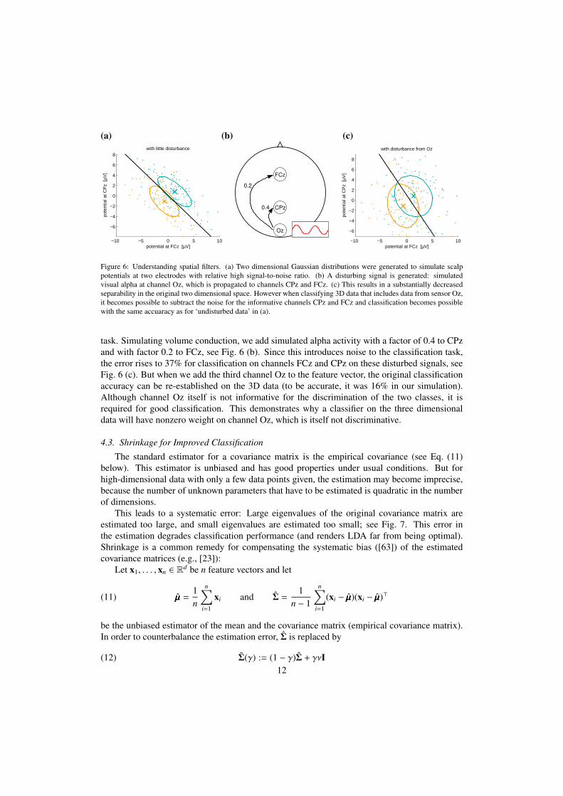
Figure 6: Understanding spatial filters. (a) Two dimensional Gaussian distributions were generated to simulate scalppotentials at two electrodes with relative high signal-to-noise ratio. (b) A disturbing signal is generated: simulatedvisual alpha at channel Oz, which is propagated to channels CPz and FCz. (c) This results in a substantially decreasedseparability in the original two dimensional space. However when classifying 3D data that includes data from sensor Oz,it becomes possible to subtract the noise for the informative channels CPz and FCz and classification becomes possiblewith the same accuaracy as for ‘undisturbed data’ in (a).

task. Simulating volume conduction, we add simulated alpha activity with a factor of 0.4 to CPzand with factor 0.2 to FCz, see Fig. 6 (b). Since this introduces noise to the classification task,the error rises to 37% for classification on channels FCz and CPz on these disturbed signals, seeFig. 6 (c). But when we add the third channel Oz to the feature vector, the original classificationaccuracy can be re-established on the 3D data (to be accurate, it was 16% in our simulation).Although channel Oz itself is not informative for the discrimination of the two classes, it isrequired for good classification. This demonstrates why a classifier on the three dimensionaldata will have nonzero weight on channel Oz, which is itself not discriminative.

4.3. Shrinkage for Improved Classification

The standard estimator for a covariance matrix is the empirical covariance (see Eq. (11)below). This estimator is unbiased and has good properties under usual conditions. But forhigh-dimensional data with only a few data points given, the estimation may become imprecise,because the number of unknown parameters that have to be estimated is quadratic in the numberof dimensions.

This leads to a systematic error: Large eigenvalues of the original covariance matrix areestimated too large, and small eigenvalues are estimated too small; see Fig. 7. This error inthe estimation degrades classification performance (and renders LDA far from being optimal).Shrinkage is a common remedy for compensating the systematic bias ([63]) of the estimatedcovariance matrices (e.g., [23]):

Let x1, . . . , xn ∈ Rd be n feature vectors and let

(11) µµµ =1n

n∑i=1

xi and Σ =1

n − 1

n∑i=1

(xi − µµµ)(xi − µµµ)>

be the unbiased estimator of the mean and the covariance matrix (empirical covariance matrix).In order to counterbalance the estimation error, Σ is replaced by

(12) Σ(γ) := (1 − γ)Σ + γνI12

0 50 100 150 200

0

50

100

150

200

250

index of Eigenvector

Eig

enva

lue

trueN=500N=200N=100N= 50

samples

Σ^

Σ

true cov.

emp. cov

Σ(0.5)∼

Σ^

νΙ

Figure 7: Left: Eigenvalue spectrum of a given covariance matrix (bold line) and eigenvalue spectra of covariancematrices estimated from a finite number of samples drawn (N= 50, 100, 200, 500) from a corresponding Gaussiandistribution. Middle: Data points drawn from a Gaussian distribution (gray dots; d = 200 dimensions, two dimensionsselected for visualization) with true covariance matrix indicated by an orange colored ellipsoid, and estimated covariancematrix in cyan. Right: An approximation of the true covariance matrix can be obtained as a linear interpolation betweenthe empirical covariance matrix and a sphere of approriate size.

for a tuning parameter γ ∈ [0, 1] and ν defined as average eigenvalue trace(Σ)/d of Σ withd being the dimensionality of the feature space. Then the following holds. Since Σ is positivesemi-definite we have an eigenvalue decomposition Σ = VDV> with orthonormal V and diagonalD. Due to the orthogonality of V we get

Σ = (1 − γ)VDV> + γνI = (1 − γ)VDV> + γνVIV> = V ((1 − γ)D + γνI) V>

as eigenvalue decomposition of Σ. That means

• Σ and Σ have the same eigenvectors (columns of V)

• extreme eigenvalues (large or small) are modified (shrunk or elongated) towards the aver-age ν.

• γ = 0 yields unregularized LDA, γ = 1 assumes spherical covariance matrices.

Using LDA with such modified covariance matrix is termed covariance-regularized LDA, regu-larized LDA or LDA with shrinkage.

For the trade-off with respect to the shrinkage parameter, recently an analytic method tocalculate the optimal shrinkage parameter for certain directions of shrinkage was found ([36];see also [70] for the first application in BCI). This approach aims at minimizing the Frobeniusnorm between the shrunk covariance matrix and the unknown true covariance matrix Σ. In effect,large sample-to-sample variance of entries in the empirical covariance are penalized, i.e., lead tostronger shrinkage. When we denote by (xk)i resp. (µµµ)i the i-th element of the vector xk resp. µµµand denote by si j the element in the i-th row and j-th column of Σ and define

zi j(k) = ((xk)i − (µµµ)i) ((xk) j − (µµµ) j),

then the optimal parameter for shrinkage towards identity (as defined by (12)) can be calculated

13

as ([58])

(13) γ? =n

(n − 1)2

∑di, j=1 vark(zi j(k))∑

i, j s2i j +∑

i(sii − ν)2.

The usage of the eq. (13) for the selection of the shrinkage parameter does not neccessarilylead to better classification results, compared to a selection based on, e.g., cross-validation, butis easier to implement and computationally much cheaper. Using regularized LDA for retrainingthe classifier after each trial during online operation as in [69] would hardly be possible withoutthe analytical solution.

With respect to classification of ERP features, we know from Fig. 5 that the shrinkage param-eter γ controls the weight vector of the corresponding classifier between the two extreme polesof spatial pattern (difference between ERPs) for γ = 1 and a spatial filter that incorporates thespatial structure of the noise for γ = 0. The latter case is optimal, if the covariance of the noise isknown. The empirical estimates that can be calculated from training data are error prone, in par-ticular for high-dimensional feature spaces. In this case, the automatic selection of the shrinkageparameter provides a good trade-off of using the spatial structure of the noise without overfittingto the particular statistics found in the training set.

The method of regularized LDA with shrinkage parameter selected by the analytical solutionof [58] is called shrinkage LDA.

5. Classification of ERP Components

We start by exploring ERP classification separately in the temporal and in the spatial domain.The purpose of classification on temporal features is to determine which channels contributemost to the discrimination task. And classifcation on spatial features demonstrates which timeintervals are most important. Taken together, this investigation provides a good idea of whichcomponents of the EEG is exploited by the classifier, and gives a better understanding of the dataand the classification process. For the actual classification task, the full information of spatio-temporal features should be exploited, as demonstrated in Section 5.3.

5.1. Classification in the Temporal Domain

ERPs exhibit a particular time course at electrodes over its generators. The temporal featurescalculated from single channels have been introduced in Section 2.1.

This single channel data does (in most cases) not contain sufficient information for a com-petitive classification. Nevertheless, we can gain useful information in the following way. Foreach single channel the classification accuracy that can be obtained from temporal features withordinary LDA is determined (e.g. by cross validation, cf. [38]). The resulting accuracy valuescan be visualized as scalp topography and provide thus a survey of the spatial distribution ofdiscriminative information, see Fig. 8 (a). In this case, we can see that relevant information orig-inates from central locations (P3), but even much better discriminability is provided by occipitalregions (vN2 component). The fact that classification in the matrix speller is mainly based onvisual evoked potentials rather than the P3 was only recently reported [68, 3]. The separabilitymap found here is completely in line with neurophysiological plausibility, but in other paradigmsit might indicate the need for further preprocessing of the signals.

14

(a) (b) (c)[%]

15

20

25

30

35

40

>=45

0 200 400 600 800 10000

10

20

30

40

time [ms]cl

assi

ficat

ion

loss

[%

]

[a.u.]

−0.06

−0.04

−0.02

0

0.02

0.04

0.06

Figure 8: Temporal and Spatial Classification. (a) The classification error of temporal features extracted from the timeinterval 115–535 ms was determined for each single channel. The obtained values are visualized here as scalp topographyby spatially interpolating the values assigned to each channel position and displaying the result as color coded map.(b) The classification error of spatial features was determined for each time interval of 30 ms duration, shifted from 0 to1000 ms. (c) Classifier as spatial filter: A linear classifier was trained on spatial features extracted from the time interval220–250 ms (shaded in subplot (b)) of the running example data set. The resulting weight vector can be visualized as atopography and can regarded as a spatial filter.

5.2. Classification in the Spatial Domain

ERPs exhibit a particular spatial distribution during the peak times of their subcomponents.Spatial features calculated from single time points (or potential values obtained by averagingwithin a given time interval) have been introduced in Section 2.1. Depending on the experimen-tal setting, classification of such spatial feature may already yield powerful classification, givenan appropriate selection of the time interval. But there is often a complex of several ERP com-ponents that contribute to the classification. In that case, spatio-temporal features can enhancethe result, see Section 5.3.

For spatial features, a classifier with ‘maximum’ shrinkage (γ = 1) uses the pattern of thedifference of the two classes as projection vector, see also Fig. 5. This corresponds to a rathersmooth topography, and might therefore seem neurophysiologically more plausibe. The moreintricate spatial filters we get with little shrinkage account for the spatial structure of the noiseand hold therefore the potential of more accurate classification, see Fig. 9 and the discussionin Section 4.2. In this sense, the shrinkage parameter reflects our belief in the estimation of thenoise. If the noise (covariance matrix) can be estimated very well, it should be taken into accountfor classification without restriction (γ = 0, i.e., ordinary LDA). But if the spatial structure ofthe noise cannot be reliably estimated from the training data one should disbelief it and shrinktowards the no-noise assumption (γ = 1) in order to avoid overfitting. The procedure for theselection of the shrinkage parameter γ provides a trade-off, that was found to work well forclassification of ERP components.

Fig. 11 (left part) shows the classification results of spatial features extracted at different timeintervals for the example data set using ordinary LDA (the right panel of that figure is explainedin the next section).

5.3. Classification in the Spatio-Temporal Domain

A good way to get an overview of where the discriminative information lies in the spatio-temporal plane is to visualize a matrix of separability measures to the spatio-temporal featuresof the experimental conditions. More specifically, this matrix is obtained by calculating a sep-arability index separately for each pair of channel and time point. In this paper, we will use

15

γ = 0 γ = 0.001 γ = 0.005 γ = 0.05 γ = 0.5 γ = 1

15

20

25

30

35

40

erro

r [%

]

[a.u.]−1 −0.8 −0.6 −0.4 −0.2 0 0.2 0.4 0.6 0.8 1

Figure 9: Results for different values of shrinkage parameter γ. Classification accuracy of spatial features (time interval205–235 ms) was evaluated for different values of shrinkage parameter γ. The normal vector of the classifier’s separatinghyperplane w can be regarded as a spatial filter (see Section 3 and 4.2) and is visualized here for each value of γ as scalpmap (arbitrary unit). For γ = 1, the normal vector w is proportional to µ2 − µ1, while it is proportional to Σ−1(µµµ2 −µµµ1) inthe case without shrinkage (γ = 0). Note, that for illustration reasons, shrinkage was applied here to spatial features, i.e.,data which is not so high-dimensional. Therefore, the gain obtained by shrinkage is not as huge as it often is for higherdimensional data, see below the result for spatio-temporal features.

16

[ms]

chan

nels

−100 0 100 200 300 400 500

Fz

FCz

Cz

CPz

Pz

Oz

115 − 135 ms 135 − 155 ms 155 − 195 ms 205 − 235 ms 285 − 325 ms 335 − 395 ms 495 − 535 ms

[a.u

.]

−0.2

−0.1

0

0.1

0.2

Figure 10: Visualization of signed r2-matrix. For the spatio-temporal features, signed r2-values of targets minus nontargetsingle trial ERPs were calculated and displayed as a color coded matrix. A heuristic was used to determine the indicatedtime intervals, which accumulate high r2 values and each time interval has a fairly constant spatial pattern of r2-values.The time-averaged r2-values for each of those intervals are also visualized as scalp topography. Note, that the matrixvisualization also shows propagation of components. The visual N1 component with peak around 175 ms at electrodesPO7 and PO8 seems to originate from frontal areas around 115 ms (light blue band going from top (= frontal areas)diagonally down to the bottom (= occipital areas)). The central P2 component peaking around 220 ms is initially morefocussed to the central area and propagates from there to frontal and occipital sites.

signed-r2-values: The pointwise biserial correlation coefficient (r-value) is defined as

(14) r(x) :=√

N1 · N2

N1 + N2

mean{xi | yi = 1} −mean{xi | yi = 2}std{xi}

,

and the signed-r2-values are sgn-r2(x) := sign(x) · r(x)2. Alternatively, other measures of separa-bility of distributions can be used, such as Fisher score ([21, 45]), Student’s t-statistic ([65, 45])area under the ROC curve ([24]) or rank-biserial correlation coefficient ([15]). The latter twomeasures have the advantage that they do not rely on the assumption that the class distributionsare Gaussian. On the other hand, since LDA assumes Gaussian distributions, it seems appropriateto make the same assumption in feature selection.

The analysis result for our example data set is shown in Fig. 10. Based on the displayedmatrix of separability indices (here, r2 values), it is possible to determine a set of time intervals({T1, . . . ,Tn} in our notions of Section 2.1) that are good candidates for classification. Sincewithin each interval the average across time is calculated, see Eq. (2), the intervals should bechosen such that within each interval the spatial pattern is fairly constant. Due to the high di-mensionality of spatio-temporal features it is important to use the shrinkage technique presentedin Section 4.3 for classification.

Fig. 11 (right part) shows the classification results for spatio-temporal features. While ordi-nary LDA suffered from overfitting and obtained a result of 25% error, which is worse than mostsingle interval results, shrinkage greatly reduced the error to only 4%. While the results of ordi-nary LDA was disappointing in this particular example data set, we would like to point out, thatLDA is in many cases a powerful and robust classification method. In the example used here,the number of training samples was low (750) compared to the dimensionality of the features(7 × 55 = 385), since this requires the estimation of 385 × 384/2 = 73, 920 parameters in the

17

−5

0

5

vP1 N1 vN1 P2 vN2 P3

N3

115−135 ms 135−155 ms 155−195 ms 205−235 ms 285−325 ms 335−395 ms 495−535 ms

10

15

20

25

30

35

err

or

[%

]

Combined

LDA

withshrinkage

5%[ V]µ

Figure 11: Classification error: (left) using spatial features extracted from different time intervals; (right) using spatio-temporal features obtained from all eight time intervals. While LDA (red circle) obtains a result that is worse than mostsingle interval results due to overfitting, shrinkage (magenta colored circle) greatly reduces the error to about 4%. Theintervals correspond to the shaded areas in Fig. 2. Bottom row: Scalp maps show the spatial distribution of the ERPcomponents in the corresponding time intervals.

covariance matrix. Additionally, to the bias in the estimation of the covariance matrix, there isalso a numerical problem in the inversion of a badly conditioned matrix. There are ways to copewith these numerical issues, e.g., involving singular value decomposition, but since that is alsokind of regularization, we did not use such a method for comparison here.

Finally, we would like to point out that the weight vector of a linear classifier trained onspatio-temporal features can be visualized similar as for spatial features, see Fig. 8 (c), but asa sequence for scalp maps that represent the resulting spatial filters for each of the chosen timeintervals Ti.

6. Empirical Evaluation

Finally, we demonstrate the effect of shrinkage on ERP detection performance and presentclassification results, validated on data of all 13 participants for both types of speller paradigms,Hex-o-Spell and the Matrix Speller, see Section 2.

In this context, we restrict the analysis to the binary classification problem target vs. non-target and provide validation results for a varying number of training samples, which nicelydemonstrates the effect of degrading performance in cases of small samples-to-feature ratios andits remedy by shrinkage.

We compare shrinkage LDA with ordinary LDA and also with stepwise LDA (SWLDA,[20]), because the latter is the state-of-the-art algorithm for the Matrix Speller resp. ERP classi-fication in some BCI groups (e.g., [31, 32, 22]). In [32] different classification algorithms havebeen compared with the conclusion that SWLDA has the greatest potential for the usage in theMatrix Speller. The SWLDA classifier was extended in [28] into an ensemble framework withsome improvement in performance, evaluated for the case of sufficient training data.

This SWLDA classifier is basically another regularized version of LDA, performing dimen-sionality reduction by restricting the number of used features (variables). Model estimation forSWLDA is done in a greedy manner by iteratively inserting and removing features from the

18

model based on statistical tests until the maximal number of active variables is reached. Themethod has three free parameters to choose: two p-values guiding insertion and removal of vari-ables, and the maximal number of variables. We here use pins = 0.1 and prem = 0.15, and amaximum of 60 predictors, as recommended in [32].

6.1. Data preprocessing and feature selection

The continuous EEG recordings of each of the 13 participants were epoched and aligned tothe onsets of intensification. A baseline correction was done based on the average EEG activitywithin 170ms directly preceding the stimulus. Epochs were split into a training and a test set asdescribed below. The training data were used to heuristically determine a set of seven subect-specific discriminative time intervals (see Section 5.1), which were constrained to lie between50ms and 650ms poststimulus (covering all components of potential interest, like P1, N1, P2, N3,P3, N3, see Fig. 2). For each trial, spatio-temporal features (cf. Section 2.1) have been calculatedin the following way. The mean activity in the selected intervals for 55 scalp electrodes gave riseto 55× 7 matrices X(1), . . . ,X(n), that were stacked into feature vectors x(1), . . . , x(n) of dimensionp = 385.

6.2. Performance evaluation setting

To analyze the performance of the classifiers in difficult settings of small samples-to-featureratios, we used a varying number of training samples (n) between 50 and 650. Splitting the datainto training and test set was done in a chronological fashion, taking the first part as training dataand the second part as test data. Note, that the maximum number of samples corresponds to 6symbol selection steps with 10 intensifications. The parameters of the linear classifiers are esti-mated from the training set, and applied on the test samples. The classifiers are optimized to pro-vide good separation between target epochs (participant focuses on intensified row/column/disc)and non-target epochs (participant focuses on different item). The validation error is calculatedon all left-out trials. This procedure was performed for all 13 participants separately and theerror rates were averaged.

6.3. Results

Fig. 12 depicts the results in the described validation setting. In cases with p >> n, Shrinkage-LDA clearly outperforms the other methods. For p < n the performance of SWLDA convergestowards Shrinkage-LDA, while ordinary LDA needs considerably more training samples for sta-ble operation. The peaking behaviour of the LDA performance near the ratio n/p = 1 looksstrange, but is well known in the machine learning literature, see [56, 59]. It is due to a numberof eigenvalues being very small but nonzero, which leads unfavorable numerical effects in theinversion of the empirical covariance matrix using the pseudo-inverse, see [29].

7. Conclusion

When analyzing BCI data, we typically examine the spatial patterns and filters that allow toclassify a certain brain state. In this tutorial, we identified an intuitive relation between patternsand filters in the context of regularized LDA. Furthermore, we gave two arguments for the dif-ferent nature of filters in contrast to patterns, which should provide a better understanding andinterpretation of spatial filters.

19

0 100 200 300 400 500 600 7000

10

20

30

40

Matrix Speller

# training samples

bina

ry v

alid

atio

n er

ror

[%]

0 100 200 300 400 500 600 7000

10

20

30

40

Hex−o−Spell

# training samples

LDASWLDAShrinkage−LDA

Figure 12: Classification results on spatio-temporal features for a variable number of training samples. Three differentvariants of linear discriminant classifiers have been trained on spatio-temporal features of p = 385 dimensions. Thenumber of training samples was varied from n = 50 to 650. The strange peaking behaviour of the LDA performance nearn = p is discussed in the main text. Left: Results for the Matrix Speller. Right: Results for Hex-o-Spell.

Mathematically, a key ingredient of the proposed algorithm was an accurate covariance ma-trix estimate, which is particularly hard in high dimensions. The use of a higher number ofchannels is potentially advantageous for ERP classification, but this improvement can only beturned to practice if the employed classification algorithm uses a proper regularization techniquethat allows to handle high dimensional features albeit a small number of training samples. Whilethis insight is well-known in statistics, the practical use of shrinkage for ERP decoding is noveland yields substantial improvements in predictive accuracy.

Future work will explore shrinkage estimation also for combinations of imaging features (seee.g. [18]) and for correlative measurements between different image modalities such as localfield potentials (LFP) and fMRI ([4]). Furthermore we will consider nonlinear variants, whereshrinkage could be performed in a kernel feature space ([61, 60, 46]).

Acknowledgement

We are very grateful to Nicole Krämer (Weierstrass Institute for Applied Analysis and Stochas-tics, Berlin) for pointing us to the analytic solution of the optimal shrinkage parameter for regu-larized linear discriminant analysis.

Furthermore, we are indebted to two reviewers and our colleges in the Berlin BCI group whogave valuable comments on earlier versions of the manuscript.

The studies were partly supported by the Bundesministerium für Bildung und Forschung(BMBF), Fkz 01IB001A/B, 01GQ0850, by the German Science Foundation (DFG, contractMU 987/3-1), by the European Union under the PASCAL2 Network of Excellence, ICT-216886.This publication only reflects the authors’ views. Funding agencies are not liable for any use thatmay be made of the information contained herein.

20

References

[1] Allison, B., Lüth, T., Valbuena, D., Teymourian, A., Volosyak, I., Gräser, A., 2009. BCI demographics: How many(and what kinds of) people can use an SSVEP BCI? IEEE Trans Neural Syst Rehabil EngIn revision.

[2] Belouchrani, A., Abed-Meraim, K., Cardoso, J.-F., Moulines, E., Feb 1997. A blind source separation techniqueusing second-order statistics. Signal Processing, IEEE Transactions on 45 (2), 434–444.

[3] Bianchi, L., Sami, S., Hillebrand, A., Fawcett, I. P., Quitadamo, L. R., Seri, S., Jun 2010. Which physiologicalcomponents are more suitable for visual ERP based brain-computer interface? A preliminary MEG/EEG study.Brain Topogr 23, 180–185.

[4] Bießmann, F., Meinecke, F. C., Gretton, A., Rauch, A., Rainer, G., Logothetis, N., Müller, K.-R., 2009. Temporalkernel canonical correlation analysis and its application in multimodal neuronal data analysis. Machine Learning79 (1-2), 5—27.URL http://www.springerlink.com/content/e1425487365v2227

[5] Birbaumer, N., Mar 2006. Brain-computer-interface research: coming of age. Clin Neurophysiol 117, 479–483.[6] Blankertz, B., Curio, G., Müller, K.-R., 2002. Classifying single trial EEG: Towards brain computer interfacing.

In: Diettrich, T. G., Becker, S., Ghahramani, Z. (Eds.), Advances in Neural Inf. Proc. Systems (NIPS 01). Vol. 14.pp. 157–164.

[7] Blankertz, B., Dornhege, G., Krauledat, M., Müller, K.-R., Curio, G., 2007. The non-invasive Berlin Brain-Computer Interface: Fast acquisition of effective performance in untrained subjects. Neuroimage 37 (2), 539–550.URL http://dx.doi.org/10.1016/j.neuroimage.2007.01.051

[8] Blankertz, B., Dornhege, G., Lemm, S., Krauledat, M., Curio, G., Müller, K.-R., 2006. The Berlin Brain-ComputerInterface: Machine learning based detection of user specific brain states. J Universal Computer Sci 12 (6), 581–607.

[9] Blankertz, B., Kawanabe, M., Tomioka, R., Hohlefeld, F., Nikulin, V., Müller, K.-R., 2008. Invariant commonspatial patterns: Alleviating nonstationarities in brain-computer interfacing. In: Platt, J., Koller, D., Singer, Y.,Roweis, S. (Eds.), Advances in Neural Information Processing Systems 20. MIT Press, Cambridge, MA, pp. 113–120.

[10] Blankertz, B., Krauledat, M., Dornhege, G., Williamson, J., Murray-Smith, R., Müller, K.-R., 2007. A note onbrain actuated spelling with the Berlin Brain-Computer Interface. In: Stephanidis, C. (Ed.), Universal Access inHCI, Part II, HCII 2007. Vol. 4555 of LNCS. Springer, Berlin Heidelberg, pp. 759–768.

[11] Blankertz, B., Losch, F., Krauledat, M., Dornhege, G., Curio, G., Müller, K.-R., 2008. The Berlin Brain-ComputerInterface: Accurate performance from first-session in BCI-naive subjects. IEEE Trans Biomed Eng 55 (10), 2452–2462.URL http://dx.doi.org/10.1109/TBME.2008.923152

[12] Blankertz, B., Tomioka, R., Lemm, S., Kawanabe, M., Müller, K.-R., Jan. 2008. Optimizing spatial filters for robustEEG single-trial analysis. IEEE Signal Process Mag 25 (1), 41–56.URL http://dx.doi.org/10.1109/MSP.2008.4408441

[13] Cardoso, J.-F., Souloumiac, A., 1993. Blind beamforming for non gaussian signals. IEE Proceedings-F 140, 362–370.

[14] Comon, P., 1994. Independent component analysis, a new concept? Signal Process. 36 (3), 287–314.[15] Cureton, E. E., 1956. Rank-biserial correlation. Psychometrika 21 (3), 287–290.[16] Curran, E. A., Stokes, M. J., 2003. Learning to control brain activity: A review of the production and control of

EEG components for driving brain-computer interface (BCI) systems. Brain Cogn 51, 326–336.[17] Dickhaus, T., Sannelli, C., Müller, K.-R., Curio, G., Blankertz, B., 2009. Predicting BCI performance to study BCI

illiteracy. BMC Neuroscience 2009 10, (Suppl 1):P84.[18] Dornhege, G., Blankertz, B., Curio, G., Müller, K.-R., Jun. 2004. Boosting bit rates in non-invasive EEG single-

trial classifications by feature combination and multi-class paradigms. IEEE Trans Biomed Eng 51 (6), 993–1002.URL http://dx.doi.org/10.1109/TBME.2004.827088

[19] Dornhege, G., del R. Millán, J., Hinterberger, T., McFarland, D., Müller, K.-R. (Eds.), 2007. Toward Brain-Computer Interfacing. MIT Press, Cambridge, MA.

[20] Draper, N., Smith, H., 1966. Applied regression analysis. Wiley series in probability and mathematical statistics.Wiley, New York.

[21] Duda, R. O., Hart, P. E., Stork, D. G., 2001. Pattern Classification, 2nd Edition. Wiley & Sons.[22] Farwell, L., Donchin, E., 1988. Talking off the top of your head: toward a mental prosthesis utilizing event-related

brain potentials. Electroencephalogr Clin Neurophysiol 70, 510–523.[23] Friedman, J. H., 1989. Regularized discriminant analysis. J Amer Statist Assoc 84 (405), 165–175.[24] Green, M. D., Swets, J. A., 1966. Signal detection theory and psychophysics. Krieger, Huntington, NY.[25] Guger, C., Daban, S., Sellers, E., Holzner, C., Krausz, G., Carabalona, R., Gramatica, F., Edlinger, G., Oct 2009.

How many people are able to control a P300-based brain-computer interface (BCI)? Neurosci Lett 462, 94–98.

21

[26] Guger, C., Edlinger, G., Harkam, W., Niedermayer, I., Pfurtscheller, G., 2003. How many people are able to operatean EEG-based Brain-Computer Interface (BCI)? IEEE Trans Neural Syst Rehabil Eng 11 (2), 145–147.

[27] Hong, B., Guo, F., Liu, T., Gao, X., Gao, S., Sep 2009. N200-speller using motion-onset visual response. ClinNeurophysiol 120, 1658–1666.

[28] Johnson, G. D., Krusienski, D. J., 2009. Ensemble SWLDA classifiers for the P300 speller. In: Proceedings of the13th International Conference on Human-Computer Interaction. Part II. Springer-Verlag, Berlin, Heidelberg, pp.551–557.

[29] Krämer, N., 2009. On the peaking phenomenon of the lasso in model selection, preprint available:http://arxiv.org/abs/0904.4416.

[30] Krauledat, M., Tangermann, M., Blankertz, B., Müller, K.-R., Aug 2008. Towards zero training for brain-computerinterfacing. PLoS ONE 3 (8), e2967.

[31] Krusienski, D., Sellers, E., McFarland, D., Vaughan, T., Wolpaw, J., Jan 2008. Toward enhanced P300 spellerperformance. J Neurosci Methods 167, 15–21.

[32] Krusienski, D. J., Sellers, E. W., Cabestaing, F., Bayoudh, S., McFarland, D. J., Vaughan, T. M., Wolpaw, J. R.,Dec 2006. A comparison of classification techniques for the P300 speller. J Neural Eng 3 (4), 299–305.

[33] Kübler, A., Kotchoubey, B., Dec 2007. Brain-computer interfaces in the continuum of consciousness. Curr OpinNeurol 20, 643–649.

[34] Kübler, A., Kotchoubey, B., Kaiser, J., Wolpaw, J., Birbaumer, N., 2001. Brain-computer communication: Unlock-ing the locked in. Psychol Bull 127 (3), 358–375.

[35] Kübler, A., Müller, K.-R., 2007. An introducton to brain computer interfacing. In: Dornhege, G., del R. Millán, J.,Hinterberger, T., McFarland, D., Müller, K.-R. (Eds.), Toward Brain-Computer Interfacing. MIT press, Cambridge,MA, pp. 1–25.

[36] Ledoit, O., Wolf, M., 2004. A well-conditioned estimator for large-dimensional covariance matrices. J MultivarAnal 88, 365–411.

[37] Lemm, S., Curio, G., Hlushchuk, Y., Müller, K.-R., April 2006. Enhancing the signal to noise ratio of ICA-basedextracted ERPs. IEEE Trans Biomed Eng 53 (4), 601–607.

[38] Lemm, S., Dickhaus, T., Blankertz, B., Müller, K.-R., 2010. Machine learning and pattern recognition in computa-tional neuroscience – a review. NeuroimageIn revision.

[39] Li, H., Li, Y., Guan, C., 2006. An effective BCI speller based on semi-supervised learning. Conf Proc IEEE EngMed Biol Soc 1, 1161–1164.

[40] Makeig, S., Jung, T.-P., Bell, A. J., Ghahremani, D., Sejnowski, T. J., 1997. Blind separation of auditory event-related brain responses into independent components. PNAS 94, 10979–10984.

[41] Martens, S. M., Hill, N. J., Farquhar, J., Schölkopf, B., Apr 2009. Overlap and refractory effects in a brain-computerinterface speller based on the visual P300 event-related potential. J Neural Eng 6, 026003.

[42] Meinicke, P., Kaper, M., Hoppe, F., Heumann, M., Ritter, H., 2003. Improving transfer rates in brain computerinterfacing: A case study. In: S. Becker, S. T., Obermayer, K. (Eds.), Advances in Neural Information ProcessingSystems 15. pp. 1107–1114.

[43] Müller, K.-R., Anderson, C. W., Birch, G. E., 2003. Linear and non-linear methods for brain-computer interfaces.IEEE Trans Neural Syst Rehabil Eng 11 (2), 165–169.

[44] Müller, K.-R., Blankertz, B., September 2006. Toward noninvasive brain-computer interfaces. IEEE Signal ProcessMag 23 (5), 125–128.

[45] Müller, K.-R., Krauledat, M., Dornhege, G., Curio, G., Blankertz, B., 2004. Machine learning techniques for brain-computer interfaces. Biomed Tech 49 (1), 11–22.

[46] Müller, K.-R., Mika, S., Rätsch, G., Tsuda, K., Schölkopf, B., May 2001. An introduction to kernel-based learningalgorithms. IEEE Neural Networks 12 (2), 181–201.

[47] Müller, K.-R., Tangermann, M., Dornhege, G., Krauledat, M., Curio, G., Blankertz, B., 2008. Machine learningfor real-time single-trial EEG-analysis: From brain-computer interfacing to mental state monitoring. J NeurosciMethods 167 (1), 82–90.URL http://dx.doi.org/10.1016/j.jneumeth.2007.09.022

[48] Nunez, P. L., Srinivasan, R., December 2005. Electric Fields of the Brain: The Neurophysics of EEG, 2nd Edition.Oxford University Press, USA.

[49] Parra, L., Alvino, C., Tang, A., Pearlmutter, B., Yeung, N., Osman, A., Sajda, P., Jun 2003. Single-Trial Detectionin EEG and MEG: Keeping it Linear. Neurocomputing 52-54, 177–183.

[50] Parra, L., Christoforou, C., Gerson, A., Dyrholm, M., Luo, A., Wagner, M., Philiastides, M., Sajda, P., 2008.Spatiotemporal linear decoding of brain state. IEEE Signal Process Mag 25 (1), 107–115.

[51] Parra, L. C., Spence, C. D., Gerson, A. D., Sajda, P., 2005. Recipes for the linear analysis of EEG. Neuroimage28 (2), 326–341.

[52] Pfurtscheller, G., Neuper, C., Birbaumer, N., 2005. Human Brain-Computer Interface. In: Riehle, A., Vaadia, E.(Eds.), Motor Cortex in Voluntary Movements. CRC Press, New York, Ch. 14, pp. 367–401.

22

[53] Quiroga, R., Garcia, H., 2003. Single-trial event-related potentials with wavelet denoising. Clin Neurophysiol 114,376–90.

[54] Rakotomamonjy, A., Guigue, V., Mar 2008. BCI competition III: dataset II- ensemble of SVMs for BCI P300speller. IEEE Trans Biomed Eng 55, 1147–1154.

[55] Ratcliff, R., Philiastides, M. G., Sajda, P., Apr 2009. Quality of evidence for perceptual decision making is indexedby trial-to-trial variability of the EEG. Proc Natl Acad Sci U S A 106, 6539–6544.

[56] Raudys, S., Duin, R., 1998. Expected classification error of the fisher linear classifier with pseudo-inverse covari-ance matrix. Pattern Recognition Letters 19, 385–392.

[57] Salvaris, M., Sepulveda, F., Aug 2009. Visual modifications on the P300 speller BCI paradigm. J Neural Eng 6,046011.

[58] Schäfer, J., Strimmer, K., 2005. A shrinkage approach to large-scale covariance matrix estimation and implicationsfor functional genomics. Stat Appl Genet Mol Biol 4, Article32.

[59] Schäfer, J., Strimmer, K., 2005. An empirical bayes approach to inferring large-scale a gene association networks.Bioinformatics 21 (6), 754–764.

[60] Schölkopf, B., Mika, S., Burges, C., Knirsch, P., Müller, K.-R., Rätsch, G., Smola, A., September 1999. Input spacevs. feature space in kernel-based methods. IEEE Trans Neural Netw 10 (5), 1000–1017.

[61] Schölkopf, B., Smola, A., Müller, K.-R., 1998. Nonlinear component analysis as a kernel eigenvalue problem.Neural Comput 10 (5), 1299–1319.

[62] Shenoy, P., Krauledat, M., Blankertz, B., Rao, R. P. N., Müller, K.-R., 2006. Towards adaptive classification forBCI. J Neural Eng 3 (1), R13–R23.URL http://dx.doi.org/10.1088/1741-2560/3/1/R02

[63] Stein, C., 1956. Inadmissibility of the usual estimator for the mean of a multivariate normal distribution. Proc. 3rdBerkeley Sympos. Math. Statist. Probability 1, 197-206 (1956).

[64] Stinstra, J., Peters, M., 1998. The volume conductor may act as a temporal filter on the ECG and EEG. Med BiolEng Comput 36, 711–6.

[65] Student, 1908. The probable error of a mean. Biometrika 6, 1–25.[66] Sugiyama, M., Krauledat, M., Müller, K.-R., 2007. Covariate shift adaptation by importance weighted cross vali-

dation. Journal of Machine Learning Research 8, 1027–1061.[67] Tomioka, R., Müller, K. R., 2010. A regularized discriminative framework for EEG based communication. Neu-

roimage 49, 415–432.[68] Treder, M. S., Blankertz, B., May 2010. (C)overt attention and speller design in visual attention based brain-

computer interfaces. Behavioral & Brain Functions 6, 28.[69] Vidaurre, C., Blankertz, B., 2010. Towards a cure for BCI illiteracy. Brain Topography 23, 194–198, open Access.

URL http://dx.doi.org/10.1007/s10548-009-0121-6

[70] Vidaurre, C., Krämer, N., Blankertz, B., Schlögl, A., 2009. Time domain parameters as a feature for eeg-basedbrain computer interfaces. Neural Networks 22, 1313–1319.

[71] Vidaurre, C., Schlögl, A., Cabeza, R., Scherer, R., Pfurtscheller, G., 2006. A fully on-line adaptive BCI. IEEETrans Biomed Eng 53 (6), 1214–1219.

[72] Vidaurre, C., Schlögl, A., Cabeza, R., Scherer, R., Pfurtscheller, G., 2007. Study of on-line adaptive discriminantanalysis for EEG-based brain computer interfaces. IEEE Trans Biomed Eng 54 (3), 550–556.

[73] von Bünau, P., Meinecke, F. C., Király, F., Müller, K.-R., 2009. Finding stationary subspaces in multivariate timeseries. Physical Review Letters 103, 214101.

[74] Wang, Y., Zhang, Z., Li, Y., Gao, X., Gao, S., Yang, F., Jun 2004. BCI competition 2003-data set IV: An algorithmbased on CSSD and FDA for classifying single-trial EEG. IEEE Trans Biomed Eng 51, 1081–1086.

[75] Williamson, J., Murray-Smith, R., Blankertz, B., Krauledat, M., Müller, K.-R., 2009. Designing for uncertain,asymmetric control: Interaction design for brain-computer interfaces. International Journal of Human-ComputerStudies 67 (10), 827–841.

[76] Wolpaw, J., Mar 2007. Brain-computer interfaces as new brain output pathways. J Physiol 579, 613–619.[77] Wolpaw, J. R., Birbaumer, N., McFarland, D. J., Pfurtscheller, G., Vaughan, T. M., 2002. Brain-computer interfaces

for communication and control. Clin Neurophysiol 113 (6), 767–791.[78] Ziehe, A., Müller, K.-R., Nolte, G., Mackert, B.-M., Curio, G., January 2000. Artifact reduction in magnetoneu-

rography based on time-delayed second-order correlations. IEEE Trans Biomed Eng 47 (1), 75–87.

23