singular value decomposition - lecture notes
TRANSCRIPT
Definitions and Notations Singular Value Decomposition Theorem Applications Summary
Singular Value DecompositionWhy and How
Royi Avital1
1Signal Processing Algorithms DepartmentElectromagnetic Area
Missile DivisionRafael
June, 2011
Definitions and Notations Singular Value Decomposition Theorem Applications Summary
1 Definitions and NotationsNotationsDefinitionsIntroduction
2 Singular Value Decomposition TheoremSVD TheoremProof of the SVD TheoremSVD PropertiesSVD Example
3 ApplicationsOrder ReductionSolving Linear Equation SystemTotal Least SquaresPrincipal Component Analysis
Definitions and Notations Singular Value Decomposition Theorem Applications Summary
Notations
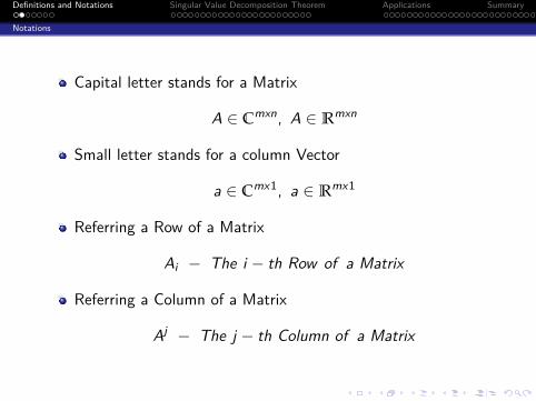
Capital letter stands for a Matrix
A ∈ Cmxn, A ∈ Rmxn
Small letter stands for a column Vector
a ∈ Cmx1, a ∈ Rmx1
Referring a Row of a Matrix
Ai − The i − th Row of a Matrix
Referring a Column of a Matrix
Aj − The j − th Column of a Matrix
Definitions and Notations Singular Value Decomposition Theorem Applications Summary
Definitions
1 Definitions and NotationsNotationsDefinitionsIntroduction
2 Singular Value Decomposition TheoremSVD TheoremProof of the SVD TheoremSVD PropertiesSVD Example
3 ApplicationsOrder ReductionSolving Linear Equation SystemTotal Least SquaresPrincipal Component Analysis
Definitions and Notations Singular Value Decomposition Theorem Applications Summary
Definitions
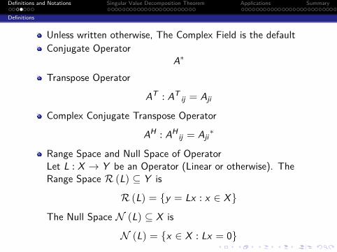
Unless written otherwise, The Complex Field is the defaultConjugate Operator
A∗
Transpose Operator
AT : ATij = Aji
Complex Conjugate Transpose Operator
AH : AHij = Aji
∗
Range Space and Null Space of OperatorLet L : X → Y be an Operator (Linear or otherwise). TheRange Space R (L) ⊆ Y is
R (L) = {y = Lx : x ∈ X}
The Null Space N (L) ⊆ X is
N (L) = {x ∈ X : Lx = 0}
Definitions and Notations Singular Value Decomposition Theorem Applications Summary
Introduction
1 Definitions and NotationsNotationsDefinitionsIntroduction
2 Singular Value Decomposition TheoremSVD TheoremProof of the SVD TheoremSVD PropertiesSVD Example
3 ApplicationsOrder ReductionSolving Linear Equation SystemTotal Least SquaresPrincipal Component Analysis
Definitions and Notations Singular Value Decomposition Theorem Applications Summary
Introduction
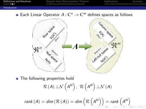
Each Linear Operator A : Cn → Cm defines spaces as follows
The following properties hold
R (A)⊥N(
AH), R
(AH)⊥N (A)
rank (A) = dim (R (A)) = dim(R(
AH))
= rank(
AH)
Definitions and Notations Singular Value Decomposition Theorem Applications Summary
Introduction
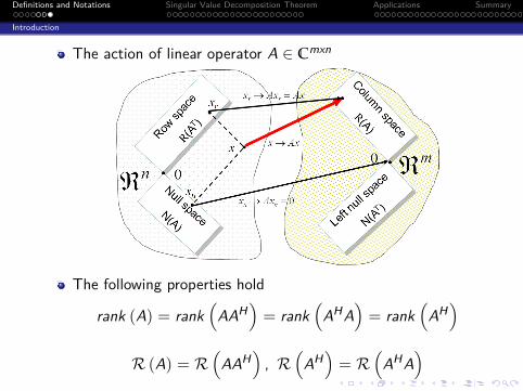
The action of linear operator A ∈ Cmxn
The following properties hold
rank (A) = rank(
AAH)= rank
(AHA
)= rank
(AH)
R (A) = R(
AAH), R
(AH)= R
(AHA
)
Definitions and Notations Singular Value Decomposition Theorem Applications Summary
SVD Theorem
1 Definitions and NotationsNotationsDefinitionsIntroduction
2 Singular Value Decomposition TheoremSVD TheoremProof of the SVD TheoremSVD PropertiesSVD Example
3 ApplicationsOrder ReductionSolving Linear Equation SystemTotal Least SquaresPrincipal Component Analysis
Definitions and Notations Singular Value Decomposition Theorem Applications Summary
SVD Theorem
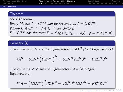
TheoremSVD Theorem:Every Matrix A ∈ Cmxn can be factored as A = UΣV H .Where U ∈ Cmxm, V ∈ Cnxn are Unitary.Σ ∈ Cmxn has the form Σ = diag (σ1, σ2, . . . , σp) , p = min (m, n).
Corollary (i)The columns of U are the Eigenvectors of AAH (Left Eigenvectors).
AAH = UΣV H(
UΣV H)H
= UΣV HV ΣHUH = UΣΣHUH
The columns of V are the Eigenvectors of AHA (RightEigenvectors).
AHA =(
UΣV H)H
UΣV H = V ΣHUHUΣV H = V ΣH ΣV H
Definitions and Notations Singular Value Decomposition Theorem Applications Summary
SVD Theorem
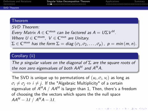
TheoremSVD Theorem:Every Matrix A ∈ Cmxn can be factored as A = UΣV H .Where U ∈ Cmxm, V ∈ Cnxn are Unitary.Σ ∈ Cmxn has the form Σ = diag (σ1, σ2, . . . , σp) , p = min (m, n).
Corollary (ii)The p singular values on the diagonal of Σ are the square roots ofthe non zero eigenvalues of both AAH and AHA.
The SVD is unique up to permutations of (ui , σi , vi ) as long asσi 6= σj ⇔ i 6= j . If the "Algebraic Multiplicity" of a certaineigenvalue of AHA / AAH is larger than 1, Then, there’s a freedomof choosing the the vectors which spans the the null spaceAAH − λI / AHA− λI.
Definitions and Notations Singular Value Decomposition Theorem Applications Summary
Proof of the SVD Theorem
1 Definitions and NotationsNotationsDefinitionsIntroduction
2 Singular Value Decomposition TheoremSVD TheoremProof of the SVD TheoremSVD PropertiesSVD Example
3 ApplicationsOrder ReductionSolving Linear Equation SystemTotal Least SquaresPrincipal Component Analysis
Definitions and Notations Singular Value Decomposition Theorem Applications Summary
Proof of the SVD Theorem
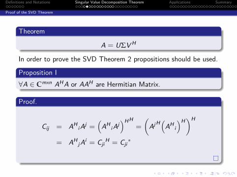
Theorem
A = UΣV H
In order to prove the SVD Theorem 2 propositions should be used.
Proposition I∀A ∈ Cmxn AHA or AAH are Hermitian Matrix.
Proof.
Cij = AHiAj =
(AH
iAj)HH
=
(Aj H(AH
i)H)H
= AHjAi = Cji
H = Cji∗
Definitions and Notations Singular Value Decomposition Theorem Applications Summary
Proof of the SVD Theorem
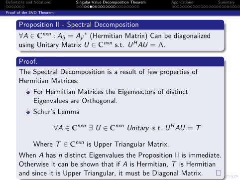
Proposition II - Spectral Decomposition∀A ∈ Cnxn : Aij = Aji
∗ (Hermitian Matrix) Can be diagonalizedusing Unitary Matrix U ∈ Cnxn s.t. UHAU = Λ.
Proof.The Spectral Decomposition is a result of few properties ofHermitian Matrices:
For Hermitian Matrices the Eigenvectors of distinctEigenvalues are Orthogonal.Schur’s Lemma
∀A ∈ Cnxn ∃ U ∈ Cnxn Unitary s.t. UHAU = T
Where T ∈ Cnxn is Upper Triangular Matrix.When A has n distinct Eigenvalues the Proposition II is immediate.Otherwise it can be shown that if A is Hermitian, T is Hermitianand since it is Upper Triangular, it must be Diagonal Matrix.
Definitions and Notations Singular Value Decomposition Theorem Applications Summary
Proof of the SVD Theorem
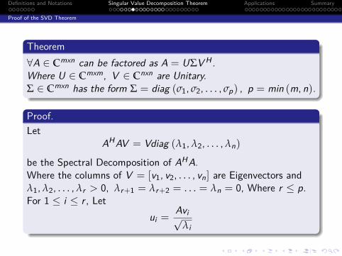
Theorem∀A ∈ Cmxn can be factored as A = UΣV H .Where U ∈ Cmxm, V ∈ Cnxn are Unitary.Σ ∈ Cmxn has the form Σ = diag (σ1, σ2, . . . , σp) , p = min (m, n).
Proof.Let
AHAV = Vdiag (λ1,λ2, . . . ,λn)
be the Spectral Decomposition of AHA.Where the columns of V = [v1, v2, . . . , vn] are Eigenvectors andλ1,λ2, . . . ,λr > 0, λr+1 = λr+2 = . . . = λn = 0, Where r ≤ p.For 1 ≤ i ≤ r , Let
ui =Avi√
λi
Definitions and Notations Singular Value Decomposition Theorem Applications Summary
Proof of the SVD Theorem
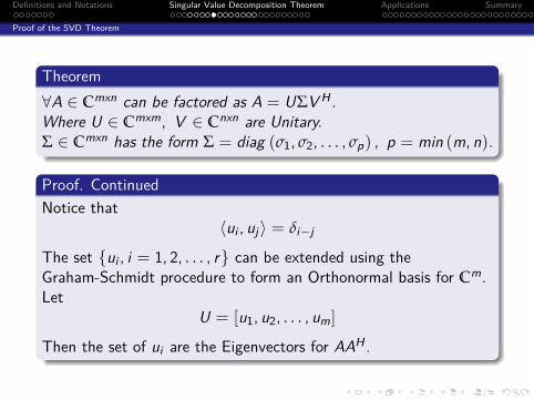
Theorem∀A ∈ Cmxn can be factored as A = UΣV H .Where U ∈ Cmxm, V ∈ Cnxn are Unitary.Σ ∈ Cmxn has the form Σ = diag (σ1, σ2, . . . , σp) , p = min (m, n).
Proof. ContinuedNotice that
〈ui , uj〉 = δi−j
The set {ui , i = 1, 2, . . . , r} can be extended using theGraham-Schmidt procedure to form an Orthonormal basis for Cm.Let
U = [u1, u2, . . . , um]
Then the set of ui are the Eigenvectors for AAH .
Definitions and Notations Singular Value Decomposition Theorem Applications Summary
Proof of the SVD Theorem
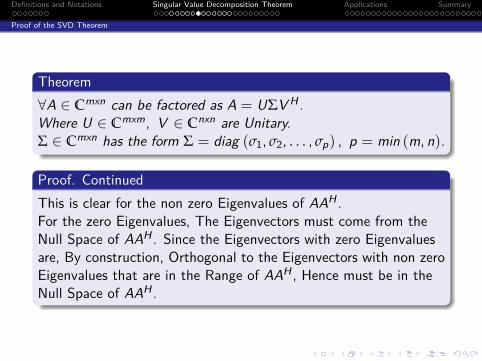
Theorem∀A ∈ Cmxn can be factored as A = UΣV H .Where U ∈ Cmxm, V ∈ Cnxn are Unitary.Σ ∈ Cmxn has the form Σ = diag (σ1, σ2, . . . , σp) , p = min (m, n).
Proof. ContinuedThis is clear for the non zero Eigenvalues of AAH .For the zero Eigenvalues, The Eigenvectors must come from theNull Space of AAH . Since the Eigenvectors with zero Eigenvaluesare, By construction, Orthogonal to the Eigenvectors with non zeroEigenvalues that are in the Range of AAH , Hence must be in theNull Space of AAH .
Definitions and Notations Singular Value Decomposition Theorem Applications Summary
Proof of the SVD Theorem
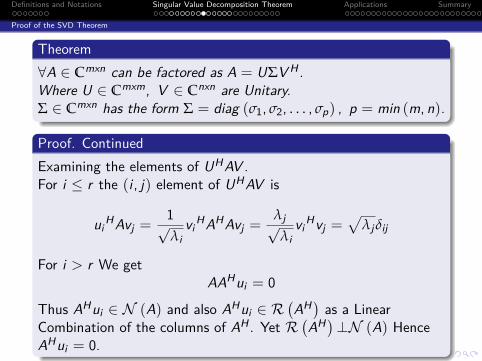
Theorem∀A ∈ Cmxn can be factored as A = UΣV H .Where U ∈ Cmxm, V ∈ Cnxn are Unitary.Σ ∈ Cmxn has the form Σ = diag (σ1, σ2, . . . , σp) , p = min (m, n).
Proof. ContinuedExamining the elements of UHAV .For i ≤ r the (i , j) element of UHAV is
uiHAvj =
1√λi
viHAHAvj =
λj√λi
viHvj =
√λj δij
For i > r We getAAHui = 0
Thus AHui ∈ N (A) and also AHui ∈ R(AH) as a Linear
Combination of the columns of AH . Yet R(AH)⊥N (A) Hence
AHui = 0.
Definitions and Notations Singular Value Decomposition Theorem Applications Summary
Proof of the SVD Theorem
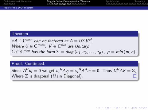
Theorem∀A ∈ Cmxn can be factored as A = UΣV H .Where U ∈ Cmxm, V ∈ Cnxn are Unitary.Σ ∈ Cmxn has the form Σ = diag (σ1, σ2, . . . , σp) , p = min (m, n).
Proof. Continued.Since AHui = 0 we get ui
HAvj = vjHAHui = 0. Thus UHAV = Σ,
Where Σ is diagonal (Main Diagonal).
Definitions and Notations Singular Value Decomposition Theorem Applications Summary
Proof of the SVD Theorem
Theorem∀A ∈ Cmxn can be factored as A = UΣV H .Where U ∈ Cmxm, V ∈ Cnxn are Unitary.Σ ∈ Cmxn has the form Σ = diag (σ1, σ2, . . . , σp) , p = min (m, n).
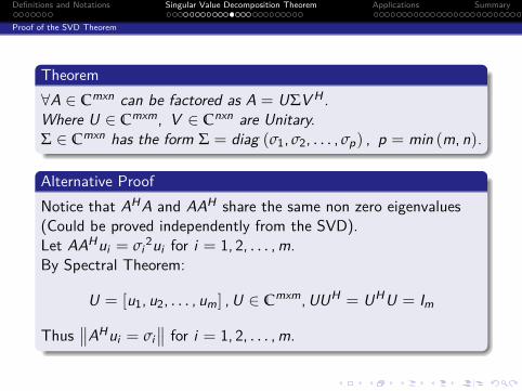
Alternative ProofNotice that AHA and AAH share the same non zero eigenvalues(Could be proved independently from the SVD).Let AAHui = σi
2ui for i = 1, 2, . . . ,m.By Spectral Theorem:
U = [u1, u2, . . . , um] ,U ∈ Cmxm,UUH = UHU = Im
Thus∥∥AHui = σi
∥∥ for i = 1, 2, . . . ,m.
Definitions and Notations Singular Value Decomposition Theorem Applications Summary
Proof of the SVD Theorem
Theorem∀A ∈ Cmxn can be factored as A = UΣV H .Where U ∈ Cmxm, V ∈ Cnxn are Unitary.Σ ∈ Cmxn has the form Σ = diag (σ1, σ2, . . . , σp) , p = min (m, n).
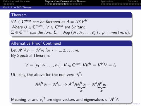
Alternative Proof ContinuedLet AHAvi = σi
2vi for i = 1, 2, . . . ,m.By Spectral Theorem:
V = [v1, v2, . . . , vm] ,V ∈ Cnxn,VV H = V HV = In
Utilizing the above for the non zero σi2:
AAHui = σi2ui ⇒ AHAAHui︸ ︷︷ ︸
zi
= σi2AHui︸ ︷︷ ︸
zi
Meaning zi and σi2 are eigenvectors and eigenvalues of AHA.
Definitions and Notations Singular Value Decomposition Theorem Applications Summary
Proof of the SVD Theorem
Theorem∀A ∈ Cmxn can be factored as A = UΣV H .Where U ∈ Cmxm, V ∈ Cnxn are Unitary.Σ ∈ Cmxn has the form Σ = diag (σ1, σ2, . . . , σp) , p = min (m, n).
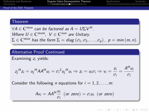
Alternative Proof ContinuedExamining zi yields:
zjHzi = uj
HAAHui = σi2uj
Hui ⇒ zi = ui σi ⇒ vi =ziσi
=AHui
σi
Consider the following n equations for i = 1, 2, . . . ,m:
Avi = AAH uiσi
(or zero) = σiui (or zero)
Definitions and Notations Singular Value Decomposition Theorem Applications Summary
Proof of the SVD Theorem
Theorem∀A ∈ Cmxn can be factored as A = UΣV H .Where U ∈ Cmxm, V ∈ Cnxn are Unitary.Σ ∈ Cmxn has the form Σ = diag (σ1, σ2, . . . , σp) , p = min (m, n).
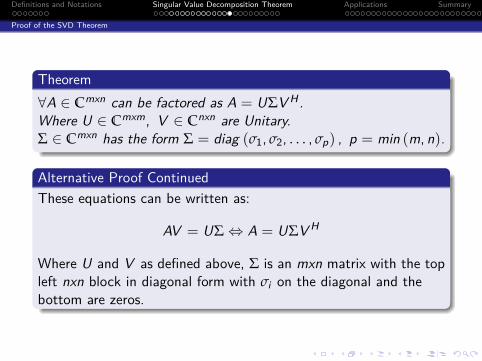
Alternative Proof ContinuedThese equations can be written as:
AV = UΣ⇔ A = UΣV H
Where U and V as defined above, Σ is an mxn matrix with the topleft nxn block in diagonal form with σi on the diagonal and thebottom are zeros.
Definitions and Notations Singular Value Decomposition Theorem Applications Summary
SVD Properties
1 Definitions and NotationsNotationsDefinitionsIntroduction
2 Singular Value Decomposition TheoremSVD TheoremProof of the SVD TheoremSVD PropertiesSVD Example
3 ApplicationsOrder ReductionSolving Linear Equation SystemTotal Least SquaresPrincipal Component Analysis
Definitions and Notations Singular Value Decomposition Theorem Applications Summary
SVD Properties
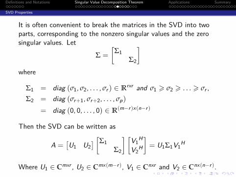
It is often convenient to break the matrices in the SVD into twoparts, corresponding to the nonzero singular values and the zerosingular values. Let
Σ =
[Σ1
Σ2
]where
Σ1 = diag (σ1, σ2, . . . , σr ) ∈ Rrxr and σ1 > σ2 > . . . > σr ,
Σ2 = diag (σr+1, σr+2, . . . , σp)
= diag (0, 0, . . . , 0) ∈ R(m−r)x(n−r)
Then the SVD can be written as
A =[U1 U2
] [Σ1Σ2
] [V1
H
V2H
]= U1Σ1V1
H
Where U1 ∈ Cmxr , U2 ∈ Cmx(m−r), V1 ∈ Cnxr and V2 ∈ Cnx(n−r).
Definitions and Notations Singular Value Decomposition Theorem Applications Summary
SVD Properties
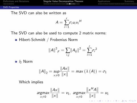
The SVD can also be written as
A =r
∑i=1
σiuiviH
The SVD can also be used to compute 2 matrix norms:Hibert-Schmidt / Frobenius Norm
‖A‖2F = ∑i ,j‖Aij‖2 =
r
∑i=1
σi2
l2 Norm
‖A‖2 = supx 6=0
‖Ax‖‖x‖ = max (λ (A)) = σ1
Which implies
argmaxx 6=0
‖Ax‖‖x‖ = v1, argmax
x 6=0
∥∥xHA∥∥
‖x‖ = u1
Definitions and Notations Singular Value Decomposition Theorem Applications Summary
SVD Properties
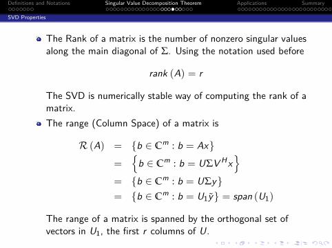
The Rank of a matrix is the number of nonzero singular valuesalong the main diagonal of Σ. Using the notation used before
rank (A) = r
The SVD is numerically stable way of computing the rank of amatrix.The range (Column Space) of a matrix is
R (A) = {b ∈ Cm : b = Ax}=
{b ∈ Cm : b = UΣV Hx
}= {b ∈ Cm : b = UΣy}= {b ∈ Cm : b = U1y} = span (U1)
The range of a matrix is spanned by the orthogonal set ofvectors in U1, the first r columns of U.
Definitions and Notations Singular Value Decomposition Theorem Applications Summary
SVD Properties
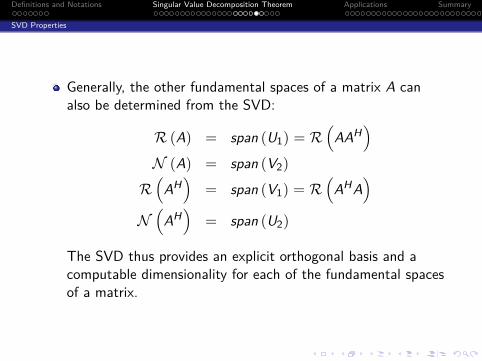
Generally, the other fundamental spaces of a matrix A canalso be determined from the SVD:
R (A) = span (U1) = R(
AAH)
N (A) = span (V2)
R(
AH)
= span (V1) = R(
AHA)
N(
AH)
= span (U2)
The SVD thus provides an explicit orthogonal basis and acomputable dimensionality for each of the fundamental spacesof a matrix.
Definitions and Notations Singular Value Decomposition Theorem Applications Summary
SVD Properties
Since the SVD is a decomposition of a given matrix into 2 Unitarymatrices and a diagonal matrix, all matrices could be described asa rotation, scaling and another rotation.This intuition is a result of the properties of unitary matrices whichbasically rotate the multiplied matrix.This property is farther examined when dealing Linear Equations.
Definitions and Notations Singular Value Decomposition Theorem Applications Summary
SVD Example
1 Definitions and NotationsNotationsDefinitionsIntroduction
2 Singular Value Decomposition TheoremSVD TheoremProof of the SVD TheoremSVD PropertiesSVD Example
3 ApplicationsOrder ReductionSolving Linear Equation SystemTotal Least SquaresPrincipal Component Analysis
Definitions and Notations Singular Value Decomposition Theorem Applications Summary
SVD Example
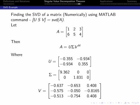
Finding the SVD of a matrix (Numerically) using MATLABcommand - [U S V] = svd(A).Let
A =
[1 2 36 5 4
]Then
A = UΣV H
WhereU =
[−0.355 −0.934−0.934 0.355
]Σ =
[9.362 0 00 1.831 0
]
V =
−0.637 −0.653 0.408−0.575 −0.050 −0.8165−0.513 −0.754 0.408
Definitions and Notations Singular Value Decomposition Theorem Applications Summary
SVD Example
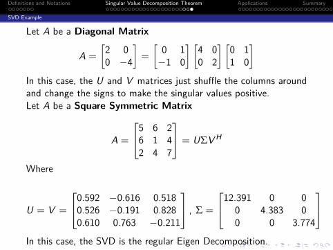
Let A be a Diagonal Matrix
A =
[2 00 −4
]=
[0 1−1 0
] [4 00 2
] [0 11 0
]In this case, the U and V matrices just shuffle the columns aroundand change the signs to make the singular values positive.Let A be a Square Symmetric Matrix
A =
5 6 26 1 42 4 7
= UΣV H
Where
U = V =
0.592 −0.616 0.5180.526 −0.191 0.8280.610 0.763 −0.211
, Σ =
12.391 0 00 4.383 00 0 3.774
In this case, the SVD is the regular Eigen Decomposition.
Definitions and Notations Singular Value Decomposition Theorem Applications Summary
Order Reduction
1 Definitions and NotationsNotationsDefinitionsIntroduction
2 Singular Value Decomposition TheoremSVD TheoremProof of the SVD TheoremSVD PropertiesSVD Example
3 ApplicationsOrder ReductionSolving Linear Equation SystemTotal Least SquaresPrincipal Component Analysis
Definitions and Notations Singular Value Decomposition Theorem Applications Summary
Order Reduction
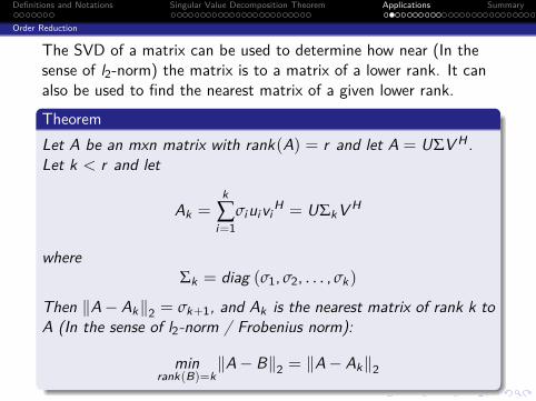
The SVD of a matrix can be used to determine how near (In thesense of l2-norm) the matrix is to a matrix of a lower rank. It canalso be used to find the nearest matrix of a given lower rank.
TheoremLet A be an mxn matrix with rank(A) = r and let A = UΣV H .Let k < r and let
Ak =k
∑i=1
σiuiviH = UΣkV H
whereΣk = diag (σ1, σ2, . . . , σk)
Then ‖A− Ak‖2 = σk+1, and Ak is the nearest matrix of rank k toA (In the sense of l2-norm / Frobenius norm):
minrank(B)=k
‖A− B‖2 = ‖A− Ak‖2
Definitions and Notations Singular Value Decomposition Theorem Applications Summary
Order Reduction
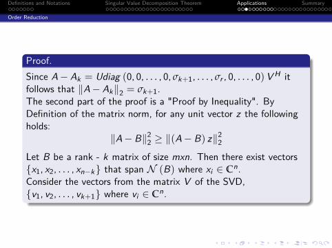
Proof.Since A− Ak = Udiag (0, 0, . . . , 0, σk+1, . . . , σr , 0, . . . , 0)V H itfollows that ‖A− Ak‖2 = σk+1.The second part of the proof is a "Proof by Inequality". ByDefinition of the matrix norm, for any unit vector z the followingholds:
‖A− B‖22 ≥ ‖(A− B) z‖22Let B be a rank - k matrix of size mxn. Then there exist vectors{x1, x2, . . . , xn−k} that span N (B) where xi ∈ Cn.Consider the vectors from the matrix V of the SVD,{v1, v2, . . . , vk+1} where vi ∈ Cn.
Definitions and Notations Singular Value Decomposition Theorem Applications Summary
Order Reduction
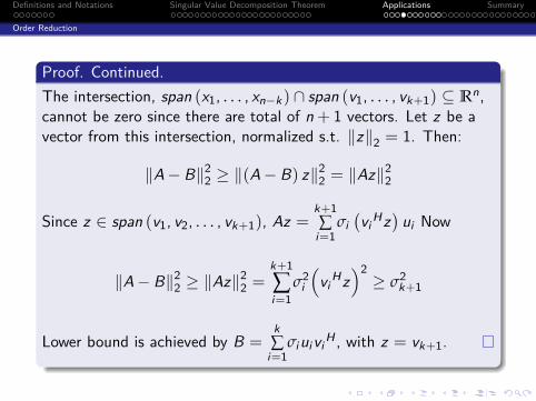
Proof. Continued.The intersection, span (x1, . . . , xn−k) ∩ span (v1, . . . , vk+1) ⊆ Rn,cannot be zero since there are total of n + 1 vectors. Let z be avector from this intersection, normalized s.t. ‖z‖2 = 1. Then:
‖A− B‖22 ≥ ‖(A− B) z‖22 = ‖Az‖22
Since z ∈ span (v1, v2, . . . , vk+1), Az =k+1∑
i=1σi(vi
Hz)
ui Now
‖A− B‖22 ≥ ‖Az‖22 =k+1
∑i=1
σ2i
(vi
Hz)2≥ σ2
k+1
Lower bound is achieved by B =k∑
i=1σiuivi
H , with z = vk+1.

Definitions and Notations Singular Value Decomposition Theorem Applications Summary
Order Reduction
Applications of Order Reduction:Image Compression
Definitions and Notations Singular Value Decomposition Theorem Applications Summary
Order Reduction
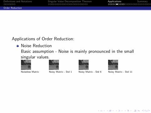
Applications of Order Reduction:Noise ReductionBasic assumption - Noise is mainly pronounced in the smallsingular values.
Noiseless Matrix Noisy Matrix - Std 1 Noisy Matrix - Std 6 Noisy Matrix - Std 11

Definitions and Notations Singular Value Decomposition Theorem Applications Summary
Order Reduction
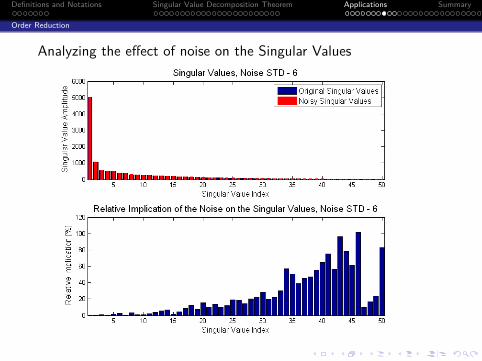
Analyzing the effect of noise on the Singular Values
Definitions and Notations Singular Value Decomposition Theorem Applications Summary
Order Reduction
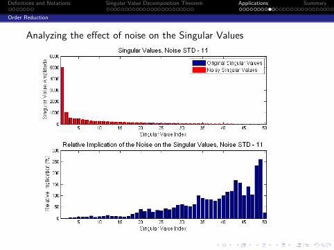
Analyzing the effect of noise on the Singular Values
Definitions and Notations Singular Value Decomposition Theorem Applications Summary
Order Reduction
Analyzing the effect of noise on the Singular Values

Definitions and Notations Singular Value Decomposition Theorem Applications Summary
Order Reduction
Ground Truth Added Noise Std 6 Reconstruction using 140 SingularValues
Definitions and Notations Singular Value Decomposition Theorem Applications Summary
Solving Linear Equation System
1 Definitions and NotationsNotationsDefinitionsIntroduction
2 Singular Value Decomposition TheoremSVD TheoremProof of the SVD TheoremSVD PropertiesSVD Example
3 ApplicationsOrder ReductionSolving Linear Equation SystemTotal Least SquaresPrincipal Component Analysis
Definitions and Notations Singular Value Decomposition Theorem Applications Summary
Solving Linear Equation System
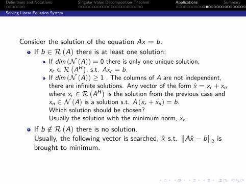
Consider the solution of the equation Ax = b.If b ∈ R (A) there is at least one solution:
If dim (N (A)) = 0 there is only one unique solution,xr ∈ R
(AH), s.t. Axr = b.
If dim (N (A)) ≥ 1 , The columns of A are not independent,there are infinite solutions. Any vector of the form x = xr + xnwhere xr ∈ R
(AH) is the solution from the previous case and
xn ∈ N (A) is a solution s.t. A (xr + xn) = b.Which solution should be chosen?Usually the solution with the minimum norm, xr .
If b /∈ R (A) there is no solution.Usually, the following vector is searched, x s.t. ‖Ax − b‖2 isbrought to minimum.
Definitions and Notations Singular Value Decomposition Theorem Applications Summary
Solving Linear Equation System
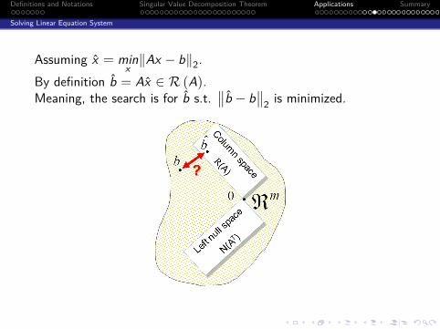
Assuming x = minx‖Ax − b‖2.
By definition b = Ax ∈ R (A).Meaning, the search is for b s.t.
∥∥b − b∥∥2 is minimized.
Definitions and Notations Singular Value Decomposition Theorem Applications Summary
Solving Linear Equation System
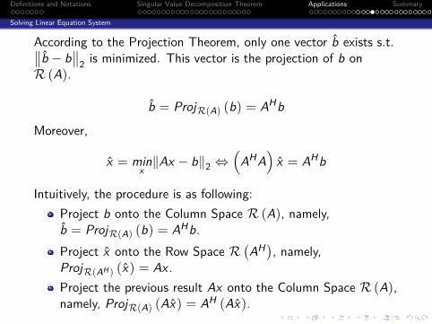
According to the Projection Theorem, only one vector b exists s.t.∥∥b − b∥∥2 is minimized. This vector is the projection of b on
R (A).
b = ProjR(A) (b) = AHb
Moreover,
x = minx‖Ax − b‖2 ⇔
(AHA
)x = AHb
Intuitively, the procedure is as following:Project b onto the Column Space R (A), namely,b = ProjR(A) (b) = AHb.Project x onto the Row Space R
(AH), namely,
ProjR(AH ) (x) = Ax .Project the previous result Ax onto the Column Space R (A),namely, ProjR(A) (Ax) = AH (Ax).
Definitions and Notations Singular Value Decomposition Theorem Applications Summary
Solving Linear Equation System
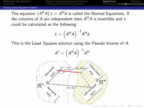
The equation(AHA
)x = AHb is called the Normal Equations. If
the columns of A are independent then AHA is invertible and xcould be calculated as the following:
x =(
AHA)−1
AHb
This is the Least Squares solution using the Pseudo Inverse of A:
A† =(
AHA)−1
AH
Definitions and Notations Singular Value Decomposition Theorem Applications Summary
Solving Linear Equation System
Yet, if the columns of A are linearly dependent the Pseudo Inverseof A can’t be calculated directly.If A has dependent columns, then the nullspace of A is not trivialand there is no unique solution.The problem becomes selecting one solution out of the infinitenumber of possible solutions.As mentioned, commonly accepted approach is to select thesolution with the smallest norm (Length).This problem could be solved using the SVD and definition of thegeneralized Pseudo Inverse of a matrix.
Definitions and Notations Singular Value Decomposition Theorem Applications Summary
Solving Linear Equation System
DefinitionThe Pseudo Inverse of a matrix A = UΣV H , denoted A† is givenby
A† = V Σ†UH
Where Σ† is obtained by transposing Σ and inverting all non zeroentries.
Proposition IIILet A = UΣV H and x † = A†b = V Σ†UHb. Then AHAx † = AHb.
Namely, using the solution given by the Pseudo Inverse matrixcalculated using the SVD holds the Normal Equations. Thisdefinition of Pseudo Inverse exists for any matrix.
Definitions and Notations Singular Value Decomposition Theorem Applications Summary
Solving Linear Equation System
Proposition IIILet A = UΣV H and x † = A†b = V Σ†UHb. Then AHAx † = AHb.
proofIt’s sufficient to show that AH (Ax † − b
)= 0.
Ax † − b =(
UΣV H)
V Σ†UHb − b
=(
UΣΣ†UH − I)
b
=(
U(
ΣΣ† − I)
UH)
b
Definitions and Notations Singular Value Decomposition Theorem Applications Summary
Solving Linear Equation System
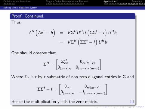
Proof. Continued.Thus,
AH(
Ax † − b)
= V ΣHUHU(
ΣΣ† − I)
UHb
= V ΣH(
ΣΣ† − I)
UHb
One should observe that
ΣH =
[ΣH
rxr 0rx(m−r)0(n−r)xr 0(m−r)x(m−r)
]Where Σr is r by r submatrix of non zero diagonal entries in Σ and
ΣΣ† − I =[
0rxr 0rx(m−r)0(n−r)xr −I (m−r)x(m−r)
]Hence the multiplication yields the zero matrix.
Definitions and Notations Singular Value Decomposition Theorem Applications Summary
Solving Linear Equation System
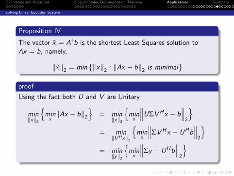
Proposition IVThe vector x = A†b is the shortest Least Squares solution toAx = b, namely,
‖x‖2 = min {‖x‖2 : ‖Ax − b‖2 is minimal}
proofUsing the fact both U and V are Unitary
min‖x‖2
{min
x‖Ax − b‖2
}= min
‖x‖2
{min
x
∥∥∥UΣV Hx − b∥∥∥2
}= min
‖V Hx‖2
{min
x
∥∥∥ΣV Hx − UHb∥∥∥2
}= min
‖y‖2
{min
x
∥∥∥Σy − UHb∥∥∥2
}
Definitions and Notations Singular Value Decomposition Theorem Applications Summary
Solving Linear Equation System
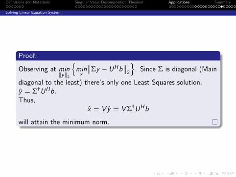
Proof.
Observing at min‖y‖2
{min
x
∥∥Σy − UHb∥∥2
}. Since Σ is diagonal (Main
diagonal to the least) there’s only one Least Squares solution,y = Σ†UHb.Thus,
x = V y = V Σ†UHb
will attain the minimum norm.
Definitions and Notations Singular Value Decomposition Theorem Applications Summary
Solving Linear Equation System
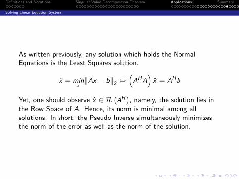
As written previously, any solution which holds the NormalEquations is the Least Squares solution.
x = minx‖Ax − b‖2 ⇔
(AHA
)x = AHb
Yet, one should observe x ∈ R(AH), namely, the solution lies in
the Row Space of A. Hence, its norm is minimal among allsolutions. In short, the Pseudo Inverse simultaneously minimizesthe norm of the error as well as the norm of the solution.
Definitions and Notations Singular Value Decomposition Theorem Applications Summary
Solving Linear Equation System
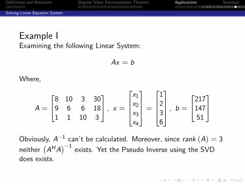
Example IExamining the following Linear System:
Ax = b
Where,
A =
8 10 3 309 6 6 181 1 10 3
, x =
x1x2x3x4
=
1236
, b =
21714751
Obviously, A−1 can’t be calculated. Moreover, since rank (A) = 3neither
(AHA
)−1 exists. Yet the Pseudo Inverse using the SVDdoes exists.
Definitions and Notations Singular Value Decomposition Theorem Applications Summary
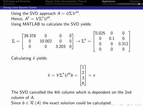
Solving Linear Equation System
Using the SVD approach A = UΣV H .Hence, A† = V Σ†UH .Using MATLAB to calculate the SVD yields:
Σ =
39.378 0 0 00 10.002 0 00 0 3.203 0
→ Σ† =
0.025 0 00 0.1 00 0 0.3120 0 0
Calculating x yields:
x = V Σ†UHb =
1236
= x
The SVD cancelled the 4th column which is dependent on the 2ndcolumn of A.Since b ∈ R (A) the exact solution could be calculated.
Definitions and Notations Singular Value Decomposition Theorem Applications Summary
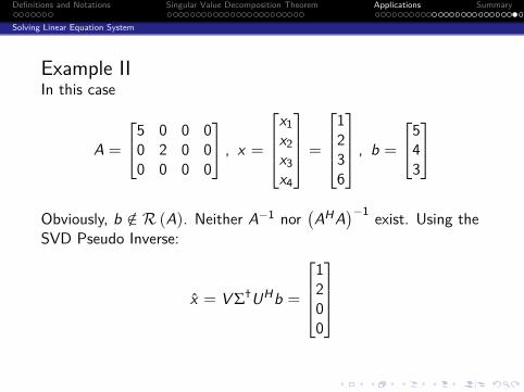
Solving Linear Equation System
Example IIIn this case
A =
5 0 0 00 2 0 00 0 0 0
, x =
x1x2x3x4
=
1236
, b =
543
Obviously, b /∈ R (A). Neither A−1 nor
(AHA
)−1 exist. Using theSVD Pseudo Inverse:
x = V Σ†UHb =
1200
Definitions and Notations Singular Value Decomposition Theorem Applications Summary
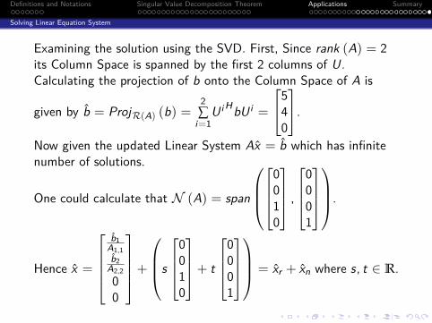
Solving Linear Equation System
Examining the solution using the SVD. First, Since rank (A) = 2its Column Space is spanned by the first 2 columns of U.Calculating the projection of b onto the Column Space of A is
given by b = ProjR(A) (b) =2∑
i=1U i HbU i =
540
.Now given the updated Linear System Ax = b which has infinitenumber of solutions.
One could calculate that N (A) = span
0010
,
0001
.
Hence x =
b1
A1,1b2
A2,200
+
s
0010
+ t
0001
= xr + xn where s, t ∈ R.
Definitions and Notations Singular Value Decomposition Theorem Applications Summary
Solving Linear Equation System
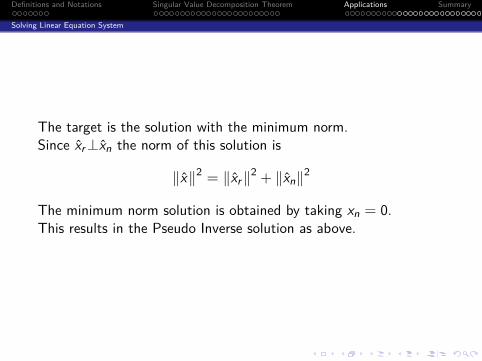
The target is the solution with the minimum norm.Since xr⊥xn the norm of this solution is
‖x‖2 = ‖xr‖2 + ‖xn‖2
The minimum norm solution is obtained by taking xn = 0.This results in the Pseudo Inverse solution as above.
Definitions and Notations Singular Value Decomposition Theorem Applications Summary
Solving Linear Equation System
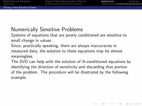
Numerically Sensitive ProblemsSystems of equations that are poorly conditioned are sensitive tosmall change in values.Since, practically speaking, there are always inaccuracies inmeasured data, the solution to these equations may be almostmeaningless.The SVD can help with the solution of ill-conditioned equations byidentifying the direction of sensitivity and discarding that portionof the problem. The procedure will be illustrated by the followingexample.
Definitions and Notations Singular Value Decomposition Theorem Applications Summary
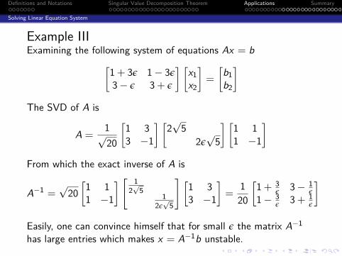
Solving Linear Equation System
Example IIIExamining the following system of equations Ax = b[
1+ 3ε 1− 3ε3− ε 3+ ε
] [x1x2
]=
[b1b2
]The SVD of A is
A =1√20
[1 33 −1
] [2√5
2ε√5
] [1 11 −1
]From which the exact inverse of A is
A−1 =√20[1 11 −1
] [ 12√5
12ε√5
] [1 33 −1
]=
120
[1+ 3
ε 3− 1ε
1− 3ε 3+ 1
ε
]Easily, one can convince himself that for small ε the matrix A−1has large entries which makes x = A−1b unstable.
Definitions and Notations Singular Value Decomposition Theorem Applications Summary
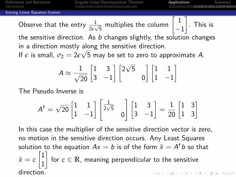
Solving Linear Equation System
Observe that the entry 12ε√5 multiplies the column
[1−1
]. This is
the sensitive direction. As b changes slightly, the solution changesin a direction mostly along the sensitive direction.If ε is small, σ2 = 2ε
√5 may be set to zero to approximate A.
A ≈ 1√20
[1 33 −1
] [2√5
0
] [1 11 −1
]The Pseudo Inverse is
A† =√20[1 11 −1
] [ 12√5
0
] [1 33 −1
]=
120
[1 31 3
]In this case the multiplier of the sensitive direction vector is zero,no motion in the sensitive direction occurs. Any Least Squaressolution to the equation Ax = b is of the form x = A†b so that
x = c[11
]for c ∈ R, meaning perpendicular to the sensitive
direction.
Definitions and Notations Singular Value Decomposition Theorem Applications Summary
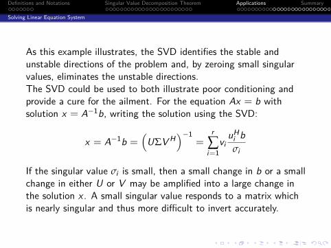
Solving Linear Equation System
As this example illustrates, the SVD identifies the stable andunstable directions of the problem and, by zeroing small singularvalues, eliminates the unstable directions.The SVD could be used to both illustrate poor conditioning andprovide a cure for the ailment. For the equation Ax = b withsolution x = A−1b, writing the solution using the SVD:
x = A−1b =(
UΣV H)−1
=r
∑i=1
viuH
i bσi
If the singular value σi is small, then a small change in b or a smallchange in either U or V may be amplified into a large change inthe solution x . A small singular value responds to a matrix whichis nearly singular and thus more difficult to invert accurately.

Definitions and Notations Singular Value Decomposition Theorem Applications Summary
Solving Linear Equation System
Another point of view, considering the equation
Ax0 = b0 ⇒ x0 = A−1b0
Let b = b0 + δb where δb is the error or noise, etc.Therefore
Ax = b0 + δb ⇒ x = A−1b0 + A−1δb = x0 + δx
Investigating how small or large is this error in the answer for agiven amount of error. Note that
δx = A−1δb ⇒ ‖δx‖ ≤∥∥A−1
∥∥ ‖δb‖
Or since∥∥A−1
∥∥ = σmax(A−1
)= 1
σmin(A) the following holds
‖δx‖ ≤ ‖δb‖σmin (A)
Definitions and Notations Singular Value Decomposition Theorem Applications Summary
Solving Linear Equation System
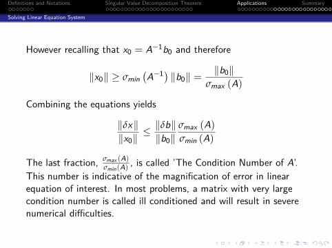
However recalling that x0 = A−1b0 and therefore
‖x0‖ ≥ σmin(A−1
)‖b0‖ =
‖b0‖σmax (A)
Combining the equations yields
‖δx‖‖x0‖
≤ ‖δb‖‖b0‖
σmax (A)σmin (A)
The last fraction, σmax (A)σmin(A) , is called ’The Condition Number of A’.
This number is indicative of the magnification of error in linearequation of interest. In most problems, a matrix with very largecondition number is called ill conditioned and will result in severenumerical difficulties.
Definitions and Notations Singular Value Decomposition Theorem Applications Summary
Solving Linear Equation System
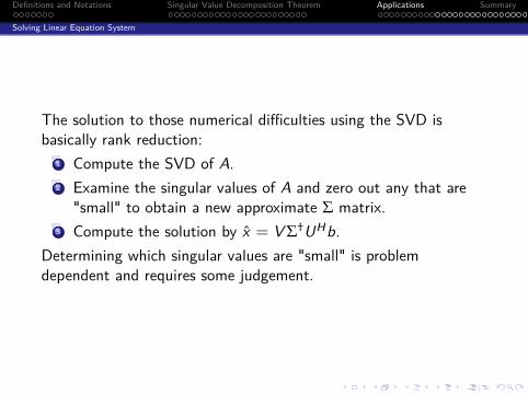
The solution to those numerical difficulties using the SVD isbasically rank reduction:
1 Compute the SVD of A.2 Examine the singular values of A and zero out any that are
"small" to obtain a new approximate Σ matrix.3 Compute the solution by x = V Σ†UHb.
Determining which singular values are "small" is problemdependent and requires some judgement.
Definitions and Notations Singular Value Decomposition Theorem Applications Summary
Total Least Squares
1 Definitions and NotationsNotationsDefinitionsIntroduction
2 Singular Value Decomposition TheoremSVD TheoremProof of the SVD TheoremSVD PropertiesSVD Example
3 ApplicationsOrder ReductionSolving Linear Equation SystemTotal Least SquaresPrincipal Component Analysis
Definitions and Notations Singular Value Decomposition Theorem Applications Summary
Total Least Squares
In the classic Least Squares problems, the solution minimizing‖Ax − b‖2 is sought after. The hidden assumption is that matrixA is correct, any error in the problem is in b.The Least Squares problem finds a vector x s.t.
‖Ax − b‖2 = min
which is accomplished by finding some perturbation r of the righthand side of minimum norm
Ax = b + r
s.t. (b + r ) ∈ R (A). In the Total Least Squares problem, boththe right and left side of the equation assumed to have errors. Thesolution of the perturbed equation
(A + E ) x = b + r
is sought s.t. (b + r ) ∈ R (A + E ) and the norm of theperturbations is minimized.
Definitions and Notations Singular Value Decomposition Theorem Applications Summary
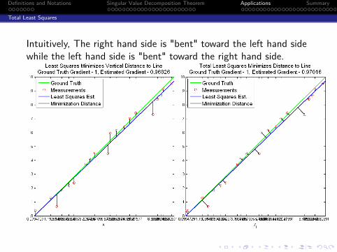
Total Least Squares
Intuitively, The right hand side is "bent" toward the left hand sidewhile the left hand side is "bent" toward the right hand side.
Definitions and Notations Singular Value Decomposition Theorem Applications Summary
Total Least Squares
Let A be an mxn matrix. To find the solution to the TLS problemone may observe the homogeneous form
[A + E |b + r
] [ x−1
]= 0→
([A|b]+[E |r]) [ x−1
]= 0
Let C =[A|b]∈ Cmx(n+1) and let ∆ =
[E |r]be the perturbation
of the data. In order for the homogeneous form to have solution
the vector[
x−1
]must lie in the Null Space of C + ∆ and in order
for the solution not to be trivial, the perturbation ∆ must be suchthat C + ∆ is rank deficient.
Definitions and Notations Singular Value Decomposition Theorem Applications Summary
Total Least Squares
Analyzing the TLS problem using the SVD. We bring(A + E ) x = (b + r ) into the form
[A + E |b + r
] [ x−1
]= 0
Let[A + E |b + r
]= UΣV H be the SVD of the above form. If
σn+1 6= 0 then rank([
A + E |b + r])
= n + 1 which means theR([
A + E |b + r])
= Rn+1, hence there’s no nonzero vector inthe orthogonal complement of the Row Space hence the set ofequations is incompatible. To obtain solution the rank of[A + E |b + r
]must be reduced to n.
As shown before the best approximation of rank n in bothFrobenius and l2 norm is given by the SVD[
A|b]= UΣV H , Σ = diag (σ1, σ2, . . . , σn, 0)
Definitions and Notations Singular Value Decomposition Theorem Applications Summary
Total Least Squares
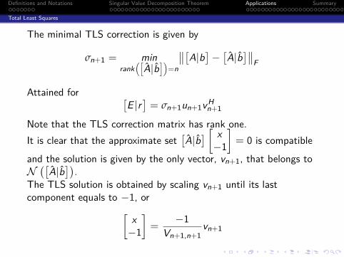
The minimal TLS correction is given by
σn+1 = minrank
([A|b
])=n
∥∥[A|b]− [A|b]∥∥F
Attained for [E |r]= σn+1un+1vH
n+1
Note that the TLS correction matrix has rank one.It is clear that the approximate set
[A|b] [ x−1
]= 0 is compatible
and the solution is given by the only vector, vn+1, that belongs toN([
A|b]).
The TLS solution is obtained by scaling vn+1 until its lastcomponent equals to −1, or[
x−1
]=
−1Vn+1,n+1
vn+1
Definitions and Notations Singular Value Decomposition Theorem Applications Summary
Total Least Squares
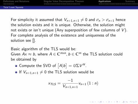
For simplicity it assumed that Vn+1,n+1 6= 0 and σn > σn+1 hencethe solution exists and it is unique. Otherwise, the solution mightnot exists or isn’t unique (Any superposition of few columns of V ).For complete analysis of the existence and uniqueness of thesolution see [].
Basic algorithm of the TLS would be:Given Ax ≈ b, where A ∈ Cmxn, b ∈ Cm the TLS solution couldbe obtained by
Compute the SVD of[A|b]= UΣV H .
If Vn+1,n+1 6= 0 the TLS solution would be
xTLS =−1
Vn+1,n+1vn+1 (1 : n)
Definitions and Notations Singular Value Decomposition Theorem Applications Summary
Total Least Squares
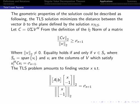
The geometric properties of the solution could be described asfollowing, the TLS solution minimizes the distance between thevector b to the plane defined by the solution xTLS .Let C = UΣV H From the definition of the l2 Norm of a matrix
‖Cv‖2‖v‖2
≥ σn+1
Where ‖v‖2 6= 0. Equality holds if and only if v ∈ Sc whereSc = span {vi} and vi are the columns of V which satisfyuH
i Cvi = σn+1.The TLS problem amounts to finding vector x s.t.∥∥∥∥[A|b] [ x
−1
]∥∥∥∥2∥∥∥∥[ x
−1
]∥∥∥∥2
= σn+1
Definitions and Notations Singular Value Decomposition Theorem Applications Summary
Total Least Squares
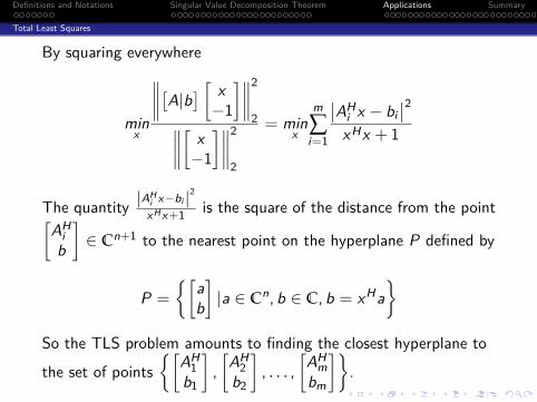
By squaring everywhere
minx
∥∥∥∥[A|b] [ x−1
]∥∥∥∥22∥∥∥∥[ x
−1
]∥∥∥∥22
= minx
m
∑i=1
∣∣AHi x − bi
∣∣2xHx + 1
The quantity |AHi x−bi |2xHx+1 is the square of the distance from the point[
AHi
b
]∈ Cn+1 to the nearest point on the hyperplane P defined by
P =
{[ab
]|a ∈ Cn, b ∈ C, b = xHa
}So the TLS problem amounts to finding the closest hyperplane to
the set of points{[
AH1
b1
],
[AH2
b2
], . . . ,
[AH
mbm
]}.
Definitions and Notations Singular Value Decomposition Theorem Applications Summary
Total Least Squares
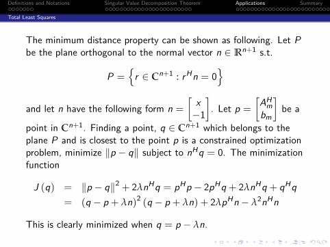
The minimum distance property can be shown as following. Let Pbe the plane orthogonal to the normal vector n ∈ Rn+1 s.t.
P ={
r ∈ Cn+1 : rHn = 0}
and let n have the following form n =
[x−1
]. Let p =
[AH
mbm
]be a
point in Cn+1. Finding a point, q ∈ Cn+1 which belongs to theplane P and is closest to the point p is a constrained optimizationproblem, minimize ‖p − q‖ subject to nHq = 0. The minimizationfunction
J (q) = ‖p − q‖2 + 2λnHq = pHp − 2pHq + 2λnHq + qHq= (q − p + λn)2 (q − p + λn) + 2λpHn− λ2nHn
This is clearly minimized when q = p − λn.
Definitions and Notations Singular Value Decomposition Theorem Applications Summary
Total Least Squares
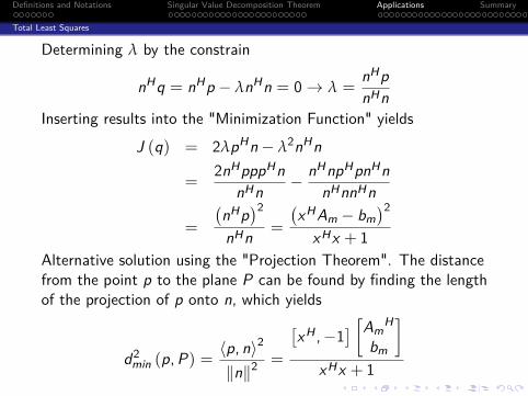
Determining λ by the constrain
nHq = nHp − λnHn = 0→ λ =nHpnHn
Inserting results into the "Minimization Function" yields
J (q) = 2λpHn− λ2nHn
=2nHpppHn
nHn − nHnpHpnHnnHnnHn
=
(nHp
)2nHn =
(xHAm − bm
)2xHx + 1
Alternative solution using the "Projection Theorem". The distancefrom the point p to the plane P can be found by finding the lengthof the projection of p onto n, which yields
d2min (p,P) =
〈p, n〉2
‖n‖2=
[xH ,−1
] [AmH
bm
]xHx + 1
Definitions and Notations Singular Value Decomposition Theorem Applications Summary
Principal Component Analysis
1 Definitions and NotationsNotationsDefinitionsIntroduction
2 Singular Value Decomposition TheoremSVD TheoremProof of the SVD TheoremSVD PropertiesSVD Example
3 ApplicationsOrder ReductionSolving Linear Equation SystemTotal Least SquaresPrincipal Component Analysis
Definitions and Notations Singular Value Decomposition Theorem Applications Summary
Principal Component Analysis
Principal Component Analysis (PCA) is the mathematicalprocedure that uses an orthogonal transformation to convert a setof observations of possibly correlated variables into a set of valuesof uncorrelated variables called Principal Components.The number of Principal Components is less than or equal to thenumber of original variables.This transformation is defined in such way that the first componenthas a variance as high as possible (That’s, accounts for as much ofthe variability in data as possible), and each succeeding componentin turn has the highest variance possible under the constraint thatit is orthogonal to (Uncorrelated with) the preceding components.
Definitions and Notations Singular Value Decomposition Theorem Applications Summary
Principal Component Analysis
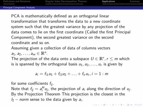
PCA is mathematically defined as an orthogonal lineartransformation that transforms the data to a new coordinatesystem such that the greatest variance by any projection of thedata comes to lie on the first coordinate (Called the first PrincipalComponent), the second greatest variance on the secondcoordinate and so on.Assuming given a collection of data of columns vectorsa1, a2, . . . , am ∈ Rn.The projection of the data onto a subspace U ∈ Rr , r ≤ m whichis is spanned by the orthogonal basis u1, u2, . . . , ur is given by
ai = fi1u1 + fi2u2 + . . . + fir ur , i = 1 : m
for some coefficients fij .Note that fij = aH
i uj , the projection of ai along the direction of uj .By the Projection Theorem This projection is the closest in thel2 − norm sense to the data given by ai .
Definitions and Notations Singular Value Decomposition Theorem Applications Summary
Principal Component Analysis
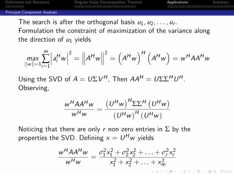
The search is after the orthogonal basis u1, u2, . . . , ur .Formulation the constraint of maximization of the variance alongthe direction of u1 yields
max‖w‖=1
m
∑i=1
∣∣∣aHi w∣∣∣2 = ∥∥∥AHw
∥∥∥2 = (AHw)H (
AHw)= wHAAHw
Using the SVD of A = UΣV H , Then AAH = UΣΣHUH .Observing,
wHAAHwwHw =
(UHw
)H ΣΣH (UHw)
(UHw)H(UHw)
Noticing that there are only r non zero entries in Σ by theproperties the SVD. Defining x = UHw yields
wHAAHwwHw =
σ21x2
1 + σ22x2
2 + . . . + σ2r x2
rx21 + x2
2 + . . . + x2m
Definitions and Notations Singular Value Decomposition Theorem Applications Summary
Principal Component Analysis
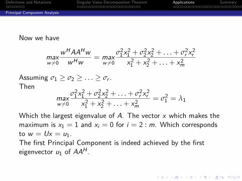
Now we have
maxw 6=0
wHAAHwwHw = max
w 6=0
σ21x2
1 + σ22x2
2 + . . . + σ2r x2
rx21 + x2
2 + . . . + x2m
Assuming σ1 ≥ σ2 ≥ . . . ≥ σr .Then
maxw 6=0
σ21x2
1 + σ22x2
2 + . . . + σ2r x2
rx21 + x2
2 + . . . + x2m
= σ21 = λ1
Which the largest eigenvalue of A. The vector x which makes themaximum is x1 = 1 and xi = 0 for i = 2 : m. Which correspondsto w = Ux = u1.The first Principal Component is indeed achieved by the firsteigenvector u1 of AAH .
Definitions and Notations Singular Value Decomposition Theorem Applications Summary
Principal Component Analysis
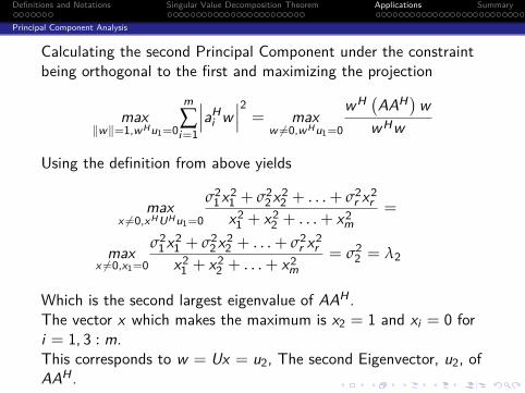
Calculating the second Principal Component under the constraintbeing orthogonal to the first and maximizing the projection
max‖w‖=1,wHu1=0
m
∑i=1
∣∣∣aHi w∣∣∣2 = max
w 6=0,wHu1=0
wH (AAH)wwHw
Using the definition from above yields
maxx 6=0,xHUHu1=0
σ21x2
1 + σ22x2
2 + . . . + σ2r x2
rx21 + x2
2 + . . . + x2m
=
maxx 6=0,x1=0
σ21x2
1 + σ22x2
2 + . . . + σ2r x2
rx21 + x2
2 + . . . + x2m
= σ22 = λ2
Which is the second largest eigenvalue of AAH .The vector x which makes the maximum is x2 = 1 and xi = 0 fori = 1, 3 : m.This corresponds to w = Ux = u2, The second Eigenvector, u2, ofAAH .
Definitions and Notations Singular Value Decomposition Theorem Applications Summary
Principal Component Analysis
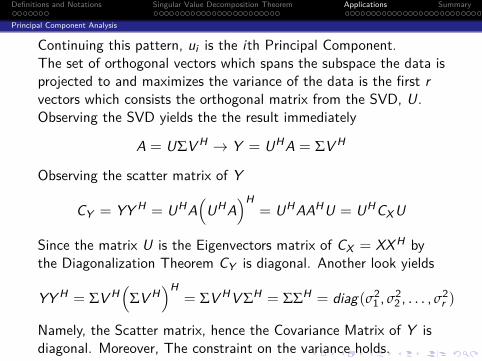
Continuing this pattern, ui is the ith Principal Component.The set of orthogonal vectors which spans the subspace the data isprojected to and maximizes the variance of the data is the first rvectors which consists the orthogonal matrix from the SVD, U.Observing the SVD yields the the result immediately
A = UΣV H → Y = UHA = ΣV H
Observing the scatter matrix of Y
CY = YY H = UHA(
UHA)H
= UHAAHU = UHCX U
Since the matrix U is the Eigenvectors matrix of CX = XXH bythe Diagonalization Theorem CY is diagonal. Another look yields
YY H = ΣV H(
ΣV H)H
= ΣV HV ΣH = ΣΣH = diag(σ21 , σ2
2 , . . . , σ2r )
Namely, the Scatter matrix, hence the Covariance Matrix of Y isdiagonal. Moreover, The constraint on the variance holds.
Definitions and Notations Singular Value Decomposition Theorem Applications Summary
The SVD is a decomposition which can be applied on anymatrix.The SVD exposes fundamental properties of a linear operatorsuch as the fundamental spaces, Frobenius Norm and l2 Norm.The SVD can be utilized in many applications such as solvinglinear systems (Least Squares, Total Least Squares) and orderreduction (Compression, Noise Reduction, PrincipalComponent Analysis).
To Be ContinuedRegulating Linear Equations System.

Appendix
For Further Reading
A. Author.Handbook of Everything.Some Press, 1990.S. Someone.On this and that.Journal on This and That. 2(1):50–100, 2000.
R. Avital.On this and that.Journal on This and That. 2(1):50–100, 2000.