sisifo · 1 introduction 1-1 overview this manual describes the characteristics of an open-source...
TRANSCRIPT

SISIFO
An open webservice for the simulation of PV systems
User manual

Page 2 of 64
INDEX
1 Introduction .................................................................................................................4
1-1 Overview ............................................................................................................. 4
1-2 Home page .......................................................................................................... 6
2 Input interface .............................................................................................................8
2-1 Introduction ........................................................................................................ 8
2-2 Site ........................................................................................................................ 9
2-3 Meteo ................................................................................................................. 10
2-4 PV modules....................................................................................................... 13
2-5 PV generator ..................................................................................................... 16
2-5-1 Ground or roof static structure ............................................................... 19
2-5-2 Façade static structure ............................................................................ 22
2-5-3 One axis horizontal or inclined tracker................................................... 24
2-5-4 One axis vertical (azimuthal) tracker...................................................... 26
2-5-5 Two axes tracker (1st vertical / 2nd horizontal) ..................................... 28
2-5-6 Two axes tracker (1st vertical / 2nd horizontal) – Venetian blind type . 30
2-5-7 Two axes tracker (1st horizontal/ 2nd perpendicular) ............................ 33
2-5-8 Delta structure......................................................................................... 35
2-6 Converters ......................................................................................................... 37
2-6-1 Inverter / Frequency Converter............................................................... 37
2-6-2 Transformer ............................................................................................ 39
2-7 Wiring ................................................................................................................ 41
2-8 Pumping ............................................................................................................ 43
2-9 Simulation options ........................................................................................... 48
2-9-1 Basic Options .......................................................................................... 48
2-9-2 Advanced Options .................................................................................. 48
2-10 Simulation time ................................................................................................ 52
2-11 Simulation ......................................................................................................... 52
3 Output interface ........................................................................................................54

Page 3 of 64
3-1 Overview ........................................................................................................... 54
3-2 Yearly parameters ............................................................................................ 54
3-3 Monthly parameters ........................................................................................ 55
3-4 Detailed Results ............................................................................................... 57
3-5 Generate technical report ............................................................................... 57
3-6 New simulation and Back to Home buttons ............................................... 57
4 ANNEX: Simulation variables ...............................................................................58
4-1 Introduction ...................................................................................................... 58
4-2 List of simulation variables ............................................................................ 58
4-2-1 Meteorological variables - Radiation on the horizontal surface ............. 58
4-2-2 Meteorological variables - Radiation on the inclined surface ................ 58
4-2-3 Meteorological variables - Daily, monthly and yearly irradiations ........ 59
4-2-4 PV system - Powers ................................................................................ 59
4-2-5 PV system - Electric energies ................................................................. 60
4-2-6 Performance ratios .................................................................................. 60
4-2-7 Other performance indices...................................................................... 61
4-2-8 PV pumping system - Instantaneous values ........................................... 61
4-2-9 PV pumping system - Daily, monthly and yearly parameters ................ 61
5 References ..................................................................................................................63

Page 4 of 64
1 Introduction
1-1 Overview This manual describes the characteristics of an open-source simulation
toolbox of PV systems in general and PV irrigation in particular, called “SISIFO”. The work of development of the simulation of PV irrigation systems has been done under the support of the European project MASLOWATEN [1].
This manual is focused on the explanation of the simulation of a PV irrigation system.
In its present version, SISIFO allows the simulation of different types of PV irrigations systems, such as the so-called, pumping systems to a water pool, or the pumping systems at constant pressure (also called direct pumping).
Figure 1 displays the general configuration of the simulated PV irrigation system, which is composed of a PV generator, a frequency converter, an AC motor and a centrifugal pump. On the other hand, Figure 2 shows the general configuration of the simulated grid-connected PV system, which includes a PV generator, an inverter and a low voltage/medium voltage (LV/MV) transformer.
Figure 1. General configuration of the simulated PV irrigation system.

Page 5 of 64
Figure 2. General configuration of the simulated grid-connected PV system.
Simulations require as input data 12 daily monthly average global horizontal irradiation and ambient temperature values, which are, at present, the most common available information for any site.
From these average values, the program is capable to generate synthetic series of daily and hourly data for the whole year.
Next the toolbox determines the irradiance on the inclined surface of the PV generator. In particular, four static surfaces and five sun-trackers (with/without backtracking option) may be simulated, which are displayed in Table 1.
Table 1. Static and tracking structures available for simulation.
Static · Ground, roof, façade, and delta (double static surface)
Tracking · One axis horizontal or inclined
· One axis vertical (azimuthal)
· Two axis (1st vertical, 2nd horizontal)
· Two axis (1st vertical, 2nd horizontal - Venetian blind type)
· Two axis (1st horizontal, 2nd perpendicular)
SISIFO simulates the behaviour of the main technology of PV modules currently present in the market (crystalline silicon (Si-c)) but in the next future, other technologies will be available such as cadmium telluride (Te-Cd), amorphous silicon (Si-a), multi-junction solar cells (e.g., III-V for concentrators) and other compound semiconductors, such as CIS/CIGS. Besides, the modeling also takes into account the effects of shading, dirt and incidence-angle losses, and spectrum.
The modelling of the system components (PV generator, frequency converter and transformer) is based on parameters that can be obtained either

Page 6 of 64
from standard information (datasheets, catalogs, specifications, etc.) or from on-site experimental measurements, and considers energy losses parameters and scenarios whose suitability has been validated in the commissioning of several PV projects carried out in Spain, Portugal, France and Italy, whose aggregated capacity is nearly 700MW.
1-2 Home page The current version of SISIFO is accessible through the following website:
http://sisifo.adminia.es/
This link gives access to the Home page displayed in Figure 3.
Figure 3. Home page of SISIFO.
At the top of the screen, there is a bar composed of different tabs. By selecting “Simulation”, the user will enter in the simulation tool and will be able to perform different simulations. By clicking “Simulation”, one has access to the input data interface and, through the webservice technology, the calculations are carried out remotely in a server that sends back the results to the remote user. At present, all the features of the tool are only available in English.
The input interface (Figure 4) is composed of several tabs (Site, Meteo Data, PV modules, PV generators, Converters, Wiring, Pumping, Options, and Time) that contain the different parameters and options that must be introduced or selected by user in order to perform a simulation. After filling all the required inputs, the user should press the red button called “Simulation” and the simulation starts.

Page 7 of 64
Figure 4. Input interface of SISIFO.
Next two chapters, called “Input interface” and “Output interface”, describe, respectively, the input parameters and the options to be selected by the user in order to perform a simulation, and the results of the simulation. Then, a list of all the simulation variables is presented. The final chapter contains the bibliographic and web references mentioned through this manual.

Page 8 of 64
2 Input interface
2-1 Introduction The top of the input interface (see Figure 4) is composed of the following
eight tabs:
- Site
- Meteo
- PV modules
- PV generators
- Converters
- Wiring
- Pumping
- Options
- Time
Besides, there is one tab called: “Simulation”, which runs a simulation.
Each of these nine tabs contains several input parameters and simulation options that must be introduced or selected by the user in order to perform a simulation, which are described below.

Page 9 of 64
2-2 Site This tab contains the geographical data of the location, which are
specified by the parameters given in Table 2.
Table 2. Geographical data of the location.
Parameters Unit Definition
Location Location of the project.
Local Latitude Degree
Latitude of the location, positive in the Northern Hemisphere and negative in the Southern Hemisphere.
Valid values: from -90 to 90
Local Altitude Meter Altitude of the location over sea level.
Local Longitude Degree Longitude of the location, negative towards West and positive towards East.
Valid values: from -180 to 180

Page 10 of 64
2-3 Meteo This tab allows selecting the “Meteo data type” and the “Sky type” that
will be used in the simulation, which are summarised in the Table 3.
“Meteo data type” may be either “Monthly averages” or “Time series” (this second option will be available soon).
Table 3. Options of METEO.
Parameters Unit Description
Meteo data type
Dimensionless Options
1 Monthly averages
2 Time series (in construction)
Sky type Dimensionless Options
1 Mean
2 Daily synthetic series
3 Hourly synthetic series
If the selected data type option is “Monthly averages”, the program generates the time series starting from the 12 monthly mean values of daily global horizontal irradiation, and maximum and minimum ambient temperatures. The first time series is automatically downloaded from the PVGIS database [2] or introduced manually by the user for the twelve months of the year (see Figure 5), while temperatures need to be introduced manually by the user. In addition, the ratio of diffuse to global irradiation can also be downloaded from PVGIS. The generation of the time series may use three different approaches, which are selected in the “Sky type” options, which are called “Mean”, “Daily synthetic series” and “Hourly synthetic series”.
The first approach, mean-sky, is the most common used in simulation software packages, and involves two steps. First, monthly mean daily horizontal global irradiation is split in beam and diffuse components, which are calculated using global-diffuse correlations, for example, those of Page [3], Erbs [4] or Macagnan [5]. These correlations are selected by the user in the “OPTIONS” tab (section 2-9).
The second step involves the estimation of the instantaneous values of beam and diffuse irradiances, which are calculated from the corresponding beam and diffuse irradiations as described by Collares-Pereira and Rabl [6].

Page 11 of 64
Figure 5. Meteo Data tab.
The second approach, “Daily synthetic series”, is rather simple to implement but, because of the monthly averaging, the weight of the medium ranges in the irradiance frequency distribution tends to be larger than the observed one. Note that as the relationship between PV output power and irradiance is affected by non-linear effects, this frequency distribution affects the PV yearly yield estimation (in some cases, up to 2-3% differences are observed).
This problem can be overcome by the synthetic generation of series of daily irradiation values by the method proposed by Aguiar-Collares. This way,
a different irradiation value, , is available for each day of the month. Then, a decomposition model, adapted to individual daily values, allows the diffuse
component, , to be derived. The four alternatives selected for such decomposition model are the following: two general polynomial relations, proposed by Collares and Erbs, the latter depending also on the sunrise angle,
, and two local correlations, proposed by Macagnan and de Miguel, for Madrid and for the Mediterranean belt, respectively. These correlations are selected by the user in the “OPTIONS” tab (section 2-9). Then, the aforementioned procedure for deriving irradiance profiles can be applied,
leading to and values for each day.

Page 12 of 64
The third approach, “Hourly synthetic series”, consists on of the direct generation of synthetic irradiance values, also following an Aguiar-Collares
proposition. This way, a series of is obtained.
Regarding to the ambient temperature, the program generates the time series starting from the monthly average of the minimum and maximum daily ambient temperatures using cosine type interpolation model [7].
Once time series of horizontal irradiances and ambient temperatures have been calculated by any of the above described methods, next steps involve the calculation of the time series of irradiances on the inclined surface of PV generators and the cell temperature, which are described, respectively in sections 2-9 (Options) and 2-4 (PV modules).

Page 13 of 64
2-4 PV modules This tab allows the selection of PV modules with different solar cell
materials, crystalline silicon and thin films (in construction), whose maximum output DC power, PDC, is calculated using the following power model:
***
ηη
GGPPDC =
Where P* is the maximum power under Standard Test Conditions (STC, defined by a normal irradiance of G*=1000W/m2 and a cell temperature of
CTC º25* = , and AM1.5 spectrum), η=η(G,TC) is the power efficiency as a function of the incident irradiance, G, and cell temperature, TC, and η* is the power efficiency under STC, η*=P*/AG*, where A is the active area of the PV generator.
Depending on the calculation of the power efficiency η, the user may select between two power models. The first one, called “Only temperature effect”, only takes into account the dependence of the efficiency with the temperature:
)(1 ** CC TT −+= γ
ηη
Where γ is the coefficient of variation of power with temperature, in ºC-1, and TC is calculated from the ambient temperature, TA, using the well know equation with the nominal operation cell temperature, NOCT, obtained from the manufacturer datasheet:
GkTGNOCTTT AAC .800
209,0 +=
−
+=
Where TA and NOCT are given in ºC, and G is given in W·m-2., and k is a thermal resistance sometimes called in the literature as Ross coefficient [8], which is given in ºC·m2/W. The experimental correction factor of 0,9 is used to consider the effect of wind speed. The factor 0.9 is an experimental correction factor, based on authors experience, which averages the cooling effect of wind speed on openback mounted PV modules. For example, for a typical value of NOCT=45ºC the previous equation gives k=0.028 ºC·m2/W.
Depending on the mounting and ventilation of the PV modules, k may typically vary from 0.02 to 0.07 ºC·m2/W. If the Ross coefficient is knew for a particular PV module and mounting, this value can also be used in the simulation calculating an “equivalent” NOCT. Table 6 displays some examples.

Page 14 of 64
In the last years, direct measurements of the cell temperature are also available from the monitoring of some grid-connected PV systems. Such measurements are normally performed either attaching a temperature sensor (thermocouple or similar) to the back surface of the modules or calculating it from the measurements of the open-circuit voltage of a reference module [9].
The second power model, called “Irradiance and temperature effects”, is now in construction, so its explanation is not included in this manual.
Table 4, Table 5 and Table 6 summarize all the parameters of this tab, while Figure 6 is an image of this input data tab.
Table 4. Available options for the PV modules tab.
Parameters Unit Definition
Cell Material Dimensionless Material of the solar cell:
Value Material
1 Si-c
2 Thin Film (in construction)
Power Model Dimensionless Power model:
Value Model
1 Only temperature effect.
2 Irradiance and temperature effects (in construction).
Table 5. Coefficients of the power module model that considers only temperature effects.
Parameters Unit Definition
CVPT %ºC-1 Coefficient of Variation of module Power with Temperature γ (absolute value).
NOCT ºC Nominal Operation Cell Temperature

Page 15 of 64
Table 6. Ross coefficient and equivalent TONC for typical mounting of PVmodules [10].
Mounting k [ºC∙m2/W] Equivalent TONC [ºC]
Well cooled 0.020 37.8
Free standing 0.021 38.5
Flat on roof 0.026 43.1
Façade integrated 0.054 67.8
On sloped roof 0.056 70.0
Figure 6. PV modules tab.

Page 16 of 64
2-5 PV generator This tab allows the selection of PV generator electrical and geometrical
characteristics.
The first parameters are electrical characteristics, which are the same for all the PV generators. They are showed in Figure 7 and defined in Table 7. The last two parameters of the table are the number of bypass diodes in the horizontal and vertical dimension, which are used by the Martinez shading model described below.
Figure 7. PV generator tab before selecting the structure.
Table 7. Electrical parameters of the PV generators.
Parameter Unit Definition
Total nominal power kWp Sum of the nominal power of all the PV generators of the system.
PV power per inverter
kWp Nominal PV power connected to a single inverter.
PV power per transformer
kWp Nominal PV power connected to each LV/MV transformer.
PRVPN Dimensionless Ratio of the real power to the nominal PV power.

Page 17 of 64
Bypass diodes – horizontal (NBGH)
Dimensionless Number of bypass diodes in the horizontal dimension.
Bypass diodes – vertical (NBGV)
Dimensionless Number of bypass diodes in the vertical dimension.
An example to correctly understand the parameters NBGH and NBGV is shown in the next figure:
+
-
+
-
+
-
NBGV = 6
+
-
+
-
+
-
+
-
+
-
+
-
+
-
+
-
+
-
NBGH=2
Figure 8. Example of the way of calculating the number of bypass diodes in the horizontal and vertical dimension.
Then, a PV structure must be selected among the four static and five sun-tracking structures available for simulation (Parameter “Struct”), which are displayed in Table 8. Once one of these structures has been selected, a list of geometrical parameters appears (Figure 9 shows an example). These parameters are particular for each structure (tilt, separation between structures, maximum rotation angles, etc.). In the case of trackers with flat-plate modules, the last parameters allow the selection of the backtracking mode of operation [11].
Table 8. Static and tracking structures available for simulation.
Static · Ground, roof, façade, and delta (double static surface)
Tracking · One axis horizontal or inclined
· One axis vertical (azimuthal)
· Two axis (1st vertical, 2nd horizontal)

Page 18 of 64
· Two axis (1st vertical, 2nd horizontal - Venetian blind type)
· Two axis (1st horizontal, 2nd perpendicular)
Figure 9. Example of a PV Generator tab: One axis horizontal.
Next sections display geometrical layouts and define the relevant parameters for each particular PV generator structure. It is worth noting that, in these layouts, all the distances are dimensionless because they are relative to the transversal dimension of the PV generator, which is indicated as “1” in the figures.

Page 19 of 64
2-5-1 Ground or roof static structure
Figure 10. Geometrical layout.
LNSNBG
V
1 (Transversal dimension)
LNS
βG
βRHorizontal
AEO
DEO
NBG
H

Page 20 of 64
Table 9. Parameters of the ground or roof PV generators.
Parameters Unit Definition
Roof inclination (βR) Degree Inclination of the roof regarding the horizontal. For a ground-mounted structure, this parameter should be zero.
Valid values: from 0 to 90
Roof orientation Degree Azimuth of the roof, which refers to either the South (Northern Hemisphere) or to the North (Southern Hemisphere). Negative towards the East and positive towards the West. For a ground-mounted structure, this parameter should be zero.
Valid values: from -90 to 90
Generator inclination (βG)
Degree Inclination of the PV generator with respect to the roof. For a ground-mounted structure, this inclination is with respect tothe horizontal.
Valid values: from 0 to 90
Generator orientation Degree Deviation of the PV generator with respect to the roof, negative towards the East and positive towards the West.
Valid values: from -90 to 90
Separation among structures N-S (LNS)
Dimensionless North-South separation among structures, specified as the ratio between this separation and transversal dimension of the PV generator.
Valid values: from 1 to 100
PV generator width (AEO)
Dimensionless Ratio of the PV generator width to its transversal dimension.
Valid values: >0
Deviation of back structure (DEO)
Dimensionless Deviation of back structure, toward the West, with respect to the front structure.
It must be provided as the ratio of this deviation to the transversal dimension of the PV generator.

Page 21 of 64
Positive towards the West and negative towards the East.
Valid values: ≥0

Page 22 of 64
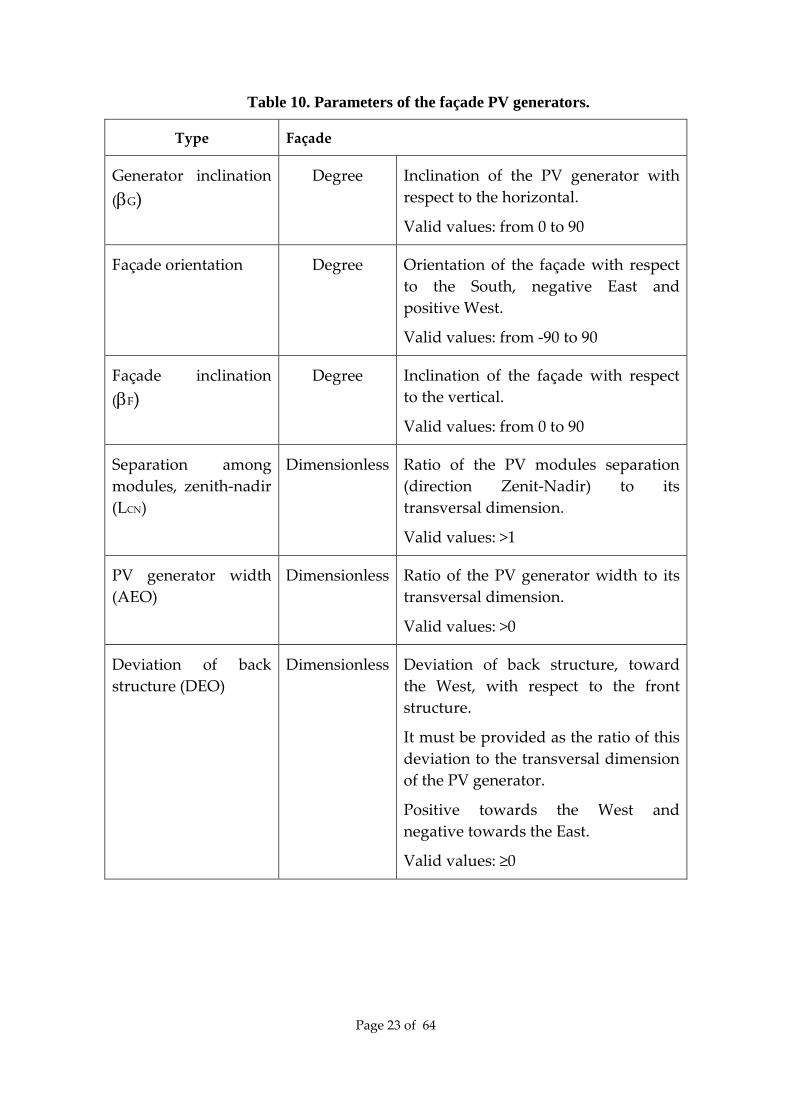
2-5-2 Façade static structure
Figure 11. Geometrical layout.
βG
1
Zenith
βF
Façade
LCN
AEO
DEO
NBGHNBGV
Page 23 of 64
Table 10. Parameters of the façade PV generators.
Type Façade
Generator inclination (βG)
Degree Inclination of the PV generator with respect to the horizontal.
Valid values: from 0 to 90
Façade orientation Degree Orientation of the façade with respect to the South, negative East and positive West.
Valid values: from -90 to 90
Façade inclination (βF)
Degree Inclination of the façade with respect to the vertical.
Valid values: from 0 to 90
Separation among modules, zenith-nadir (LCN)
Dimensionless Ratio of the PV modules separation (direction Zenit-Nadir) to its transversal dimension.
Valid values: >1
PV generator width (AEO)
Dimensionless Ratio of the PV generator width to its transversal dimension.
Valid values: >0
Deviation of back structure (DEO)
Dimensionless Deviation of back structure, toward the West, with respect to the front structure.
It must be provided as the ratio of this deviation to the transversal dimension of the PV generator.
Positive towards the West and negative towards the East.
Valid values: ≥0

Page 24 of 64
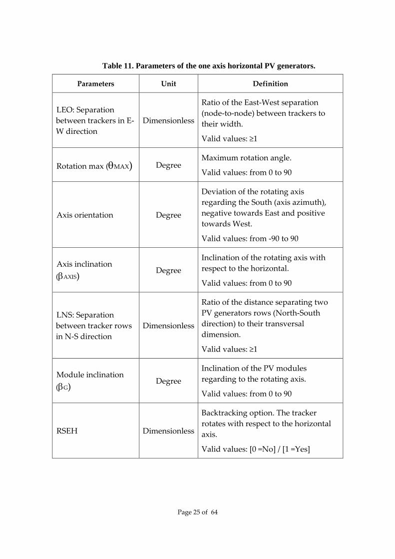
2-5-3 One axis horizontal or inclined tracker
Figure 12. Geometrical layout.
Page 25 of 64
Table 11. Parameters of the one axis horizontal PV generators.
Parameters Unit Definition
LEO: Separation between trackers in E-W direction
Dimensionless
Ratio of the East-West separation (node-to-node) between trackers to their width.
Valid values: ≥1
Rotation max (θMAX) Degree Maximum rotation angle.
Valid values: from 0 to 90
Axis orientation Degree
Deviation of the rotating axis regarding the South (axis azimuth), negative towards East and positive towards West.
Valid values: from -90 to 90
Axis inclination (βAXIS)
Degree Inclination of the rotating axis with respect to the horizontal.
Valid values: from 0 to 90
LNS: Separation between tracker rows in N-S direction
Dimensionless
Ratio of the distance separating two PV generators rows (North-South direction) to their transversal dimension.
Valid values: ≥1
Module inclination (βG) Degree
Inclination of the PV modules regarding to the rotating axis.
Valid values: from 0 to 90
RSEH Dimensionless
Backtracking option. The tracker rotates with respect to the horizontal axis.
Valid values: [0 =No] / [1 =Yes]

Page 26 of 64
2-5-4 One axis vertical (azimuthal) tracker
Figure 13. Geometrical layout.
LEO
LNS
N
1
ALARGβG
E W
S
NBGHNBGV

Page 27 of 64
Table 12. Parameters of the one axis vertical (Azimuthal) PV generators.
Parameters Unit Definition
Rack inclination (βG) Degree Inclination respect to horizontal
Valid values: from 0 to 90
LEO: Separation between trackers in E-
W direction Dimensionless
Ratio of the East-West separation (node-to-node) between trackers to their width.
Valid values: ≥1
LNS: Separation between tracker rows
in N-S direction Dimensionless
Ratio of the distance separating two PV generators rows (North-South direction) to their transversal dimension.
Valid values: ≥ALARG
Tracker height-width ratio (ALARG)
Dimensionless Ratio of the height to the width of the tracker.
Valid values: >0
RSEV Dimensionless Backtracking option. The tracker rotates with respect to the vertical axis.
Valid values: [0 =No] / [1 =Yes]

Page 28 of 64
2-5-5 Two axes tracker (1st vertical / 2nd horizontal)
Figure 14. Geometrical layout.
LEO
LNS
N
1
ALARGβMAX
E W
S
NBGHNBGV

Page 29 of 64
Table 13. Parameters of the two axis (Primary vertical / Secondary
horizontal) PV generators.
Parameters Unit Definition
Azimuth rotation angle limit
Degree Limit for azimuthal rotation angle.
Valid values: from 90 to 180
Maximum inclination (βMAX)
Degree Maximum tilt angle for the tracker.
Valid values: from 0 to 90
LEO: Separation between trackers in E-W direction
Dimensionless
Ratio of the East-West separation (node-to-node) between trackers to their width.
Valid values: ≥1
LNS: Separation between tracker rows in N-S direction
Dimensionless
Ratio of the distance separating two PV generators rows (North-South direction) to their transversal dimension.
Valid values: ≥ALARG
ALARG: Tracker height-width ratio
Dimensionless Ratio of the height to the width of the tracker.
Valid values: >0
RSEV Dimensionless
Backtracking option. regarding to the vertical axis. The tracker rotates with respect to the vertical axis.
Valid values: [0 =No] / [1 =Yes]
RSEH Dimensionless
Backtracking option. regarding to the horizontal axis. The tracker rotates with respect to the vertical axis.
Valid values: [0 =No] / [1 =Yes]

Page 30 of 64
2-5-6 Two axes tracker (1st vertical / 2nd horizontal) – Venetian blind type
Figure 15. Geometrical layout.

Page 31 of 64
Table 14. Parameters of the two axis (Primary vertical / Secondary horizontal) Venetian blind PV generators.
Parameters Unit Definition
Rack inclination (βRACK) Degree
Inclination of the rack with respect to the horizontal.
Valid values: from 0 to 90
LEO: Separation between trackers in E-W direction
Dimensionless
Ratio of the East-West separation (node-to-node) between trackers to their width.
Valid values: ≥1
LNS: Separation between tracker rows in N-S direction
Dimensionless
Ratio of the distance separating two trackers (North-South direction) to their transversal dimension.
Valid values: ≥ALARG
ALARG Dimensionless Ratio of the height to the width of the tracker.
Valid values: ≥0
RSEV Dimensionless Backtracking option. The tracker rotates with respect to vertical axis.
Valid values: [0 =No] / [1 =Yes]
RSEH Dimensionless Backtracking option. The tracker rotates with respect to horizontal axis.
Valid values: [0 =No] / [1 =Yes]
LNS_rack: Separation between rows in rack
Dimensionless
Separation of the rows in the rack, relative to the width of the tracker and measured in the rack plane.
Valid values: ≥ALARGF
ALARGF Dimensionless Ratio of the height to the width of a row in the rack
Valid values: ≥ALARG
NF Dimensionless Number of rows per tracker.

Page 32 of 64
Valid values: ≥1
NBFV Dimensionless Number of bypass diodes per row in the vertical sense.
Valid values: ≥1

Page 33 of 64
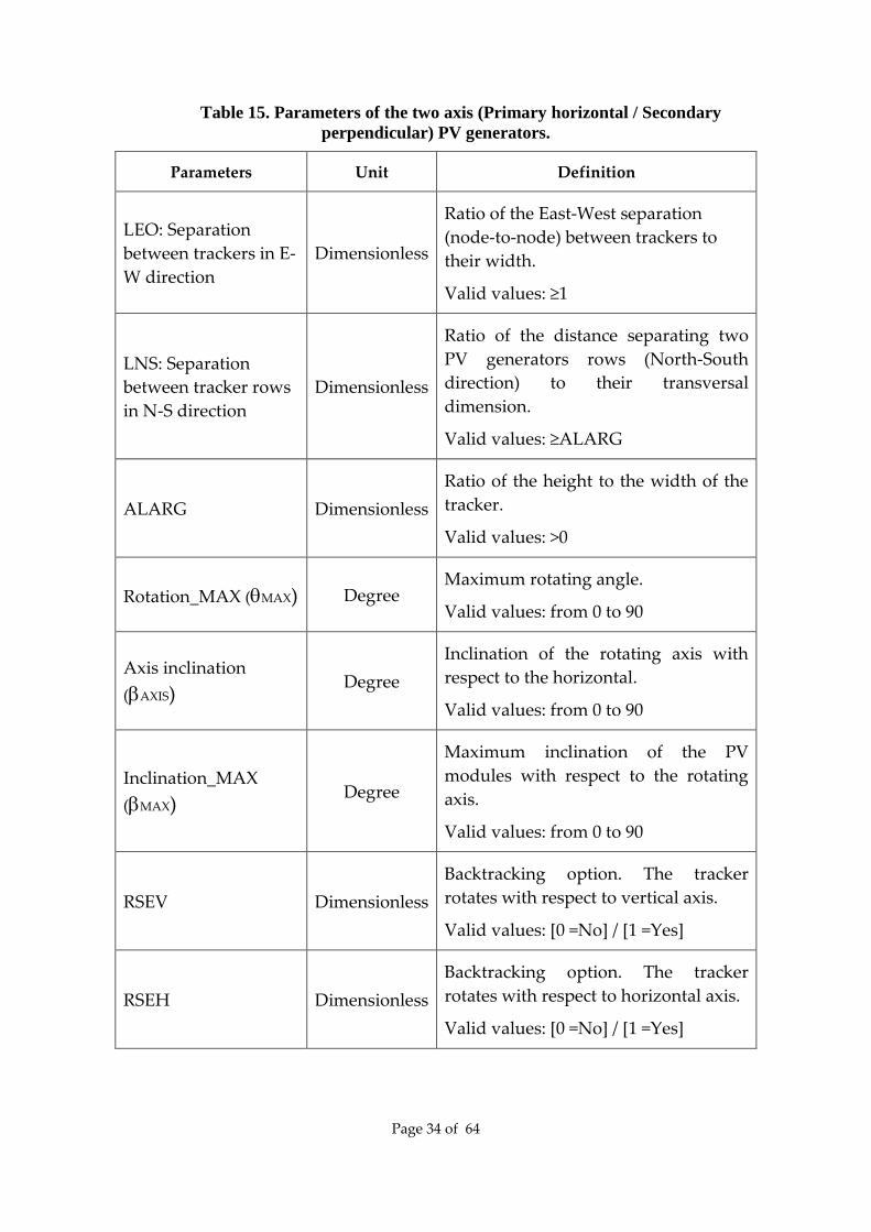
2-5-7 Two axes tracker (1st horizontal/ 2nd perpendicular)
Figure 16. Geometrical layout.
Page 34 of 64
Table 15. Parameters of the two axis (Primary horizontal / Secondary perpendicular) PV generators.
Parameters Unit Definition
LEO: Separation between trackers in E-W direction
Dimensionless
Ratio of the East-West separation (node-to-node) between trackers to their width.
Valid values: ≥1
LNS: Separation between tracker rows in N-S direction
Dimensionless
Ratio of the distance separating two PV generators rows (North-South direction) to their transversal dimension.
Valid values: ≥ALARG
ALARG Dimensionless Ratio of the height to the width of the tracker.
Valid values: >0
Rotation_MAX (θMAX) Degree Maximum rotating angle.
Valid values: from 0 to 90
Axis inclination (βAXIS)
Degree Inclination of the rotating axis with respect to the horizontal.
Valid values: from 0 to 90
Inclination_MAX (βMAX)
Degree
Maximum inclination of the PV modules with respect to the rotating axis.
Valid values: from 0 to 90
RSEV Dimensionless Backtracking option. The tracker rotates with respect to vertical axis.
Valid values: [0 =No] / [1 =Yes]
RSEH Dimensionless Backtracking option. The tracker rotates with respect to horizontal axis.
Valid values: [0 =No] / [1 =Yes]

Page 35 of 64
2-5-8 Delta structure
Figure 17. Geometrical layout.

Page 36 of 64
Table 16. Parameters of the delta generators – West oriented surface.
Parameters Unit Definition
Generator inclination (βW)
Degree Inclination of the PV generator regarding the ground.
Valid values: from 0 to 90
Separation among structures (L)
Dimensionless Separation East-West among structures, specified as the ratio between this separation and transversal dimension of the PV generator.
Valid values: ≥2
PV generator width (AEO)
Dimensionless Ratio of the PV generator width to its transversal dimension.
Total West power kWp Nominal power of the West surface.
Valid values: ≤ Total nominal Power of PV generator
Table 17. Parameters of the delta generators – East oriented surface.
Parameters Unit Definition
Generator inclination (βE)
Degree Inclination of the PV generator regarding the ground.
Valid values: from 0 to 90
Total East power kWp This value is automatically calculated and did not appear in the input interface.
Valid values: Total nominal Power of PV generator - Total West power

Page 37 of 64
2-6 Converters This tab, displayed in Figure 18, allows to select the electrical
characteristics of the inverter or frequency converter, as well as LV/MV and MV/HV transformers.
Figure 18. Converters tab.
2-6-1 Inverter / Frequency Converter The inverter is characterized by its nominal (PI) and maximum output
powers and three experimental parameters (k0, k1 and k2), which are associated, respectively, to the no-load, linear, and Joule inverter losses of the inverter. These parameters are used to calculate its power efficiency, ηI, by means of this equation [12]:
)( 2210 acacac
ac
DC
ACI pkpkkp
pPP
+++==η

Page 38 of 64
Where pac=PAC/PI, being PAC the output AC power of the inverter/frequency converter, which can be determined from PDC (power at the inverter input) and parameters k0, k1 and k2, which must be fitted either from the power efficiency curve provided by the manufacturer or from experimental measurements [13].
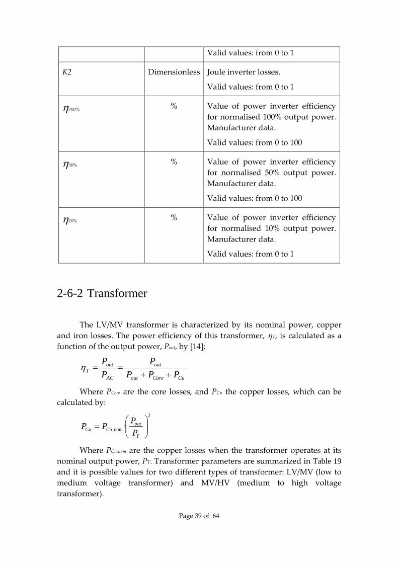
If the ki parameters are not available, they are calculated internally using the values of the power inverter efficiency curve for normalized 10%, 50% and 100% output power points obtained from the manufacturer’s information. Inverter/frequency converter parameters are summarized in Table 18.
Table 18. Inverter/Frequency converter parameters.
Parameters Unit Description
Nominal power kW Nominal power of the inverter.
Valid values: from 0,5*Total nominal Power of PV generator to 1,5*Total nominal Power of PV generator
Maximum power kW Maximum power of the inverter.
Valid values: from 0,5*Total nominal Power of PV generator to 1,5*Total nominal Power of PV generator
Auxiliary consumptions
Consumption of auxiliary equipment.
Valid values:<10% of Nominal power
Power efficiency specification
Specification of the power efficiency curve (excluding auxiliary consumptions).
Valid values: [1 =Model parameters k0, k1 and k2 ] / [2 =point of the power efficiency curve]
K0 Dimensionless No-load inverter losses.
Valid values: from 0 to 1
K1 Dimensionless Linear inverter losses.
Page 39 of 64
Valid values: from 0 to 1
K2 Dimensionless Joule inverter losses.
Valid values: from 0 to 1
η100% % Value of power inverter efficiency for normalised 100% output power. Manufacturer data.
Valid values: from 0 to 100
η50% % Value of power inverter efficiency for normalised 50% output power. Manufacturer data.
Valid values: from 0 to 100
η10% % Value of power inverter efficiency for normalised 10% output power. Manufacturer data.
Valid values: from 0 to 1
2-6-2 Transformer
The LV/MV transformer is characterized by its nominal power, copper and iron losses. The power efficiency of this transformer, ηT, is calculated as a function of the output power, Pout, by [14]:
CuCoreout
out
AC
outT PPP
PPP
++==η
Where PCore are the core losses, and PCu the copper losses, which can be calculated by:
2
, ·
=
T
outnomCuCu P
PPP
Where PCu,nom are the copper losses when the transformer operates at its nominal output power, PT. Transformer parameters are summarized in Table 19 and it is possible values for two different types of transformer: LV/MV (low to medium voltage transformer) and MV/HV (medium to high voltage transformer).

Page 40 of 64
Table 19. Transformer parameters.
Parameters Unit Description
Nominal power kW Nominal power of the transformer.
Valid values: from 0,5*Total nominal Power of PV generator to 1,5*Total nominal Power of PV generator
Iron losses kW No-load transformer losses.
Valid values:<10% of Nominal power
Copper losses kW Copper transformer losses.
Valid values:<10% of Nominal power

Page 41 of 64
2-7 Wiring
This tab (see Figure 19) contains the wiring losses, which are included in Table 20.
Wiring losses are indicated in percent of the nominal PV power and they are calculated using an equation similar to the previous one:
2
·
=
NOMWnomW P
PPP
Where PWnom are the wiring losses when the input power at the wiring section is equal to the nominal PV power, PNOM. Wiring parameters are summarized in Table 20.
Table 20. Wiring parameters.
Parameters Unit Description
WDC % DC wiring losses between PV generator and inverter at nominal PV power.
Valid values: from 0 to 10%
WBT % AC wiring losses between inverter and MV transformer at nominal PV power.
Valid values: from 0 to 10%
WMT % AC wiring losses between MV and HV transformers at nominal PV power.
Valid values: from 0 to 10%
WAT % AC wiring losses between HV transformer and the PPC at nominal PV power.
Valid values: from 0 to 10%

Page 42 of 64
Figure 19. Wiring tab.
Page 43 of 64
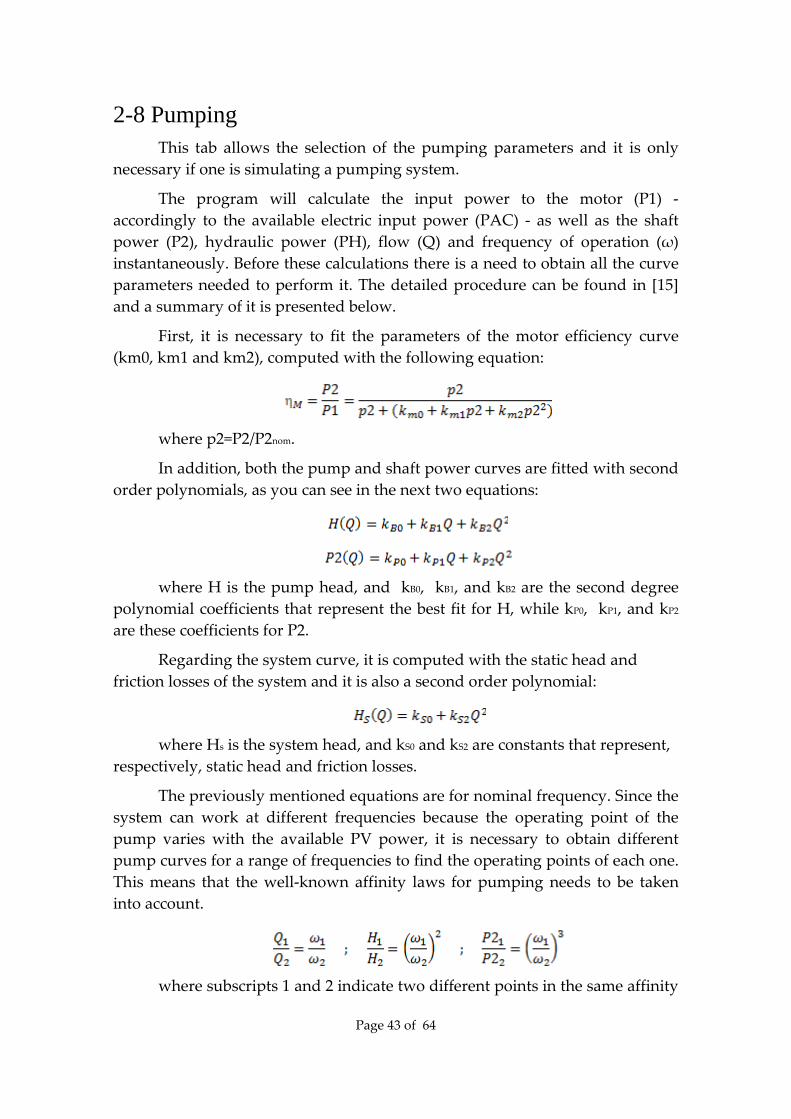
2-8 Pumping This tab allows the selection of the pumping parameters and it is only
necessary if one is simulating a pumping system.
The program will calculate the input power to the motor (P1) - accordingly to the available electric input power (PAC) - as well as the shaft power (P2), hydraulic power (PH), flow (Q) and frequency of operation (ω) instantaneously. Before these calculations there is a need to obtain all the curve parameters needed to perform it. The detailed procedure can be found in [15] and a summary of it is presented below.
First, it is necessary to fit the parameters of the motor efficiency curve (km0, km1 and km2), computed with the following equation:
where p2=P2/P2nom.
In addition, both the pump and shaft power curves are fitted with second order polynomials, as you can see in the next two equations:
where H is the pump head, and kB0, kB1, and kB2 are the second degree
polynomial coefficients that represent the best fit for H, while kP0, kP1, and kP2
are these coefficients for P2.
Regarding the system curve, it is computed with the static head and friction losses of the system and it is also a second order polynomial:
where Hs is the system head, and kS0 and kS2 are constants that represent,
respectively, static head and friction losses.
The previously mentioned equations are for nominal frequency. Since the system can work at different frequencies because the operating point of the pump varies with the available PV power, it is necessary to obtain different pump curves for a range of frequencies to find the operating points of each one. This means that the well-known affinity laws for pumping needs to be taken into account.
where subscripts 1 and 2 indicate two different points in the same affinity

Page 44 of 64
parabola and in different pump curves.
The final goal of the pump modelling is to obtain the relationship between flow (Q) and shaft power (P2), which means having access to the following equation:
where kQ0, kQ1, kQ2 and kQ3 are the third degree polynomial coefficients
that represent the best fit for Q.
In the case of the direct pumping, the operating point is unique. Even so, all the previous procedure is executed because the operating point can means a frequency different than the nominal one.
In order to perform the pumping simulation one needs to start by selecting the type of pumping: water pool or direct. For pump and motor selection, two options are available:
1. To use Caprari online catalog, or
2. To introduce data manually (without the need to use Caprari online catalog). If one is using this option it is necessary to introduce the rated flow (Qnom) and rated head (Hnom) and to provide the different points of the pump curve (H(Q)), shaft power curve (P2(Q)) and power efficiency curve (η(P2)). It is very important to mention that it is mandatory to include the point H(Q=0) in the first curve, i.e., the height at zero flow. In addition, the pumped liquid and its density, the nominal shaft power, the rated speed (as well as its minimum and maximum), the nominal frequency and the rated voltage are also required.
Then, it is necessary to insert the system curve parameters, i.e., the static head (He) and the friction losses at rated flow (Hf).
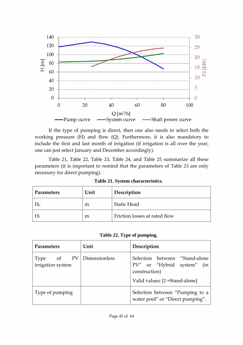
With the previous parameters, the information included in the next figure is obtained.
Page 45 of 64
If the type of pumping is direct, then one also needs to select both the
working pressure (H) and flow (Q). Furthermore, it is also mandatory to include the first and last month of irrigation (if irrigation is all over the year, one can just select January and December accordingly).
Table 21, Table 22, Table 23, Table 24, and Table 25 summarize all these parameters (it is important to remind that the parameters of Table 23 are only necessary for direct pumping).
Table 21. System characteristics.
Parameters Unit Description
He m Static Head
Hf m Friction losses at rated flow
Table 22. Type of pumping.
Parameters Unit Description
Type of PV irrigation system
Dimensionless Selection between “Stand-alone PV” or “Hybrid system” (in construction)
Valid values: [1 =Stand-alone]
Type of pumping Selection between “Pumping to a water pool” or “Direct pumping”.

Page 46 of 64
Valid values: [1 =Water pool] / [2=Direct]
Table 23. Direct pumping characteristics.
Parameters Unit Description
Working pressure m Select the working pressure of the system in terms of equivalent height (in meters)
Valid values: from 0 to the maximum height included in the pump curve
Working flow m3/h Select the working flow of the system
Valid values: from 0 to the maximum flow included in the pump curve
First month of irrigation
Select the first month of irrigation
Valid values: from 1 to 12 (month of the year)
Last month of irrigation
Select the last month of irrigation
Valid values: from 1 to 12 (month of the year)
Table 24. Pump characteristics.
Parameters Unit Description
Model Product name
Rated flow m3/h
Rated head m
Pumped liquid Type of pumped liquid
Density kg/m3 Liquid density
Pump curve Q[m3/h]
H[m]
Height for different flows (at nominal power)

Page 47 of 64
Shaft power curve Q[m3/h]
P2[kW]
Shaft power (mechanical output power of the motor) for different flows (at nominal power)
Table 25. Motor characteristics.
Parameters Unit Description
Model Product name
P2nom kW Rated shaft power
RPMnom RPM Rated speed used for pump data
RPMcool % Minimum speed, relative to the rated speed, for water cooling
RPMmax % Maximum speed, relative to the rated speed
Frequency Hz Nominal frequency
Rated voltage V
Power efficiency P2[kW]
Efficiency [%]
Efficiency for different shaft power values (at nominal power)

Page 48 of 64
2-9 Simulation options This tab (see Figure 20) contains the simulation options that can be
selected by the user, which are summarised in Table 26, at the end of this section.
Figure 20. Simulation options tab.
2-9-1 Basic Options The first two options, “Application” and “Analysis”, indicate,
respectively, the PV application to be simulated (Grid connected or Irrigation PV systems) and the type of analysis to be performed (in the current version, the simulator only performs yearly analysis).
2-9-2 Advanced Options The next options, which should be modified by advanced users, deal
with the models to be used by the sequence of algorithms, which involves two main steps. The first one is the translation of irradiance values from the horizontal surface to the plane of PV modules and second step involves the discount of power losses caused by shading, dirt, angle-of-incidence and spectrum. The transposition procedure follows the next sequence of calculations, based on previous work [11], [16]:
1. Position of the Sun, position of the PV generator surface, and incidence angle [7].

Page 49 of 64
2. Shaded area on the PV generator. If this shaded area is not null and the backtracking mode of operation has been selected, the tracker rotates on the corresponding axis to eliminate the shadow [11].
3. Irradiance on the PV generator plane using different diffuse radiation models: isotropic, Hay [17] or Perez [18], which is selected in the option “Diffuse Model”.
4. Dirt and incidence losses. The implemented model [19] calculates both types of losses and the user must select the degree of dust in the option “Soiling”.
5. Shading losses, calculated using different the model of Martinez et al. Refinement of the previous classic model using an empirical approach [20]. This model and the previous one require specifying the number of bypass diodes or blocks along the dimensions of the PV generator. Figure 21 shows an example.
6. Spectral correction [21], selected in the option “Spectral Response”.
Figure 21. Example of a PV generator composed by four modules, each one with three bypass diodes. In this example, the number of bypass diodes (or groups of cells protected by the same bypass diode) in the horizontal dimension is 2, while
in the vertical dimension is 6.
+
-
+
-
+
-
NBGV = 6
+
-
+
-
+
-
+
-
+
-
+
-
+
-
+
-
+
-
NBGH=2

Page 50 of 64
Finally, the last three options are:
“Minimum irradiance” is the threshold irradiance above which power can be injected into the grid. This parameter is usually provided by the inverter manufacturer. By default, its value is zero.
The “Ground reflectance” is the reflectance of the ground, which may vary from 0.1 for grass up to 0.8 for snow [22]. The default value is 0.2, which is the recommended value for the monthly mean of the ground reflectance when the value of this parameter is unknown.
The option “Daily diffuse correlation” is the global-diffuse model to be used in the estimation of the beam and diffuse components of the horizontal global irradiation, which is the first step of the generation of time series described in section 2-3. There are three available correlations: Page [2], Erbs [4] or Macagnan [5]. This option is only available if the option Synthetized Series of daily data is selected as Sky Type (see section METEO).
The option “Hourly diffuse correlation” is used to select the correlation used to calculate the irradiance values. This option is only available if the option Synthetized Series of hourly data is selected as Sky Type (see section METEO).
All the above described options are summarized in Table 26.
Table 26. Simulation options.
Parameters Unit Description
PV Application PV application to be simulated.
Valid values: [1 =Grid connected] / [2 =PV irrigation].
Analysis type Analysis type.
Valid values: [1 =Yearly analysis]
Soiling % Degree of Dust in %.
Valid values: from 0 to 10%
Spectral Response Dimensionless Consideration of the spectral response of the PV modules
Valid values: [0 =No] / [1 =Yes]
Diffuse Model Dimensionless Models: Isotropic, Anisotropic (Hay), and Anisotropic (Perez). The recommended one is Anisotropic

Page 51 of 64
(Perez)
Valid values:
[1 =Isotropic / [2 =Anisotropic (Hay)] / [3 =Anisotropic (Perez)].
Monthly Diffuse Correlation Dimensionless
Model for the monthly diffuse fraction (only used if Sky Type is “mean”).
Valid values:
[0 =Database / [1=Page] / [2=Collares-Pereira] / [3=Erbs] / [4=Macagnan]
Daily Diffuse Correlation Dimensionless
Model for the daily diffuse fraction (only used if Sky Type is “Daily synthetized Series”)
[0 =Database / [1=Collares-Rabl] / [2=Erbs] / [3= Macagnan] / [4=de Miguel]
Hourly Diffuse Correlation Dimensionless
Model for the hourly diffuse fraction (only used if Sky Type is “Hourly synthetized Series”). The recommended one is BRL
Valid values:
[1 =Orgill-Hollands / [2 =Erbs] / [3 =BRL] / [4 =de Miguel].
Shading Model Dimensionless Model to calculate shading losses. Valid values:
[1 =Martinez]
Minimum irradiance W/m2 Minimum irradiance required to generate power.
Valid values: from 0 to 500 W/m2
Ground Reflectance Dimensionless Ground reflectance of the surrounding floor.
Valid values: from 0 to 0.8

Page 52 of 64
2-10 Simulation time The simulation time tab (see Figure 22) allows the selection of the
number of days to be simulated:
• All the days, which performs the simulation for the 365 days of the year.
• Characteristic days, which only simulates with the characteristic day of each month (i.e., day numbers 17, 45, 74, 105, 135, 161, 199, 230, 261, 292, 322 and 347). It is in construction.
Another parameter to be selected in this tab is the “Simulation Step”, in minutes, which establishes the time resolution of the simulation. The solar time is used as time reference.
Figure 22. Simulation time tab.
2-11 Simulation Once the options are selected by the user, the simulation starts when
simulation button (in red) is pressed (see Figure 22). Next, a new tab is opened in the web browser, which shows the results of the simulation. It is worth pointing out that the simulation will only start if all the required drop-down menus are selected. These menus are indicated in Table 27.

Page 53 of 64
Table 27. Tabs of the input interface and required drop-down menus to be selected in order to perform a new simulation.
Tab Drop‐down menus
Site None.
Meteo “Data type” ,
“Sky model”.
PV modules “Solar cell material” (default: Si-c),
“Module power model” (default: only temperature effect).
PV generators “Structure”.
Converters “Power efficiency curve”.
Wiring None.
Pumping (required only for water pumping)
“Type of PV system” (default: Stand-alone),
“Type of pumping” (default: water pool),
“First month of irrigation” (default: April),
“Last month of irrigation” (default: October).
Options “PV application” (default: Water pumping),
“Analysis type” (default: Yearly Analysis),
“Spectral response” (default: Yes),
“Diffuse radiation modeling” (default: Anisotropic – Perez),
“Monthly diffuse correlation” (default: Database),
“Daily diffuse correlation” (default: Erbs),
“Hourly diffuse correlation” (default: BRL),
“Shading model” (default: Martinez).
Time “Simulation days” (default: Whole year – 1 to 365),
“Time reference” (default: Solar time).

Page 54 of 64
3 Output interface
3-1 Overview The output interface of SISIFO is a new webpage (opened in a new tab)
where different options are displayed in the main bar (see Figure 23). Here, it is possible to see yearly, monthly and detailed results. In addition, an “exit” button is presented, which will close the results tab, maintaining the simulation tab if one wants to perform a new simulation. In the following, the results visualization will be explained.
Figure 23. Output interface: part of yearly parameters
3-2 Yearly parameters The first tab, displayed in Figure 23, shows the following yearly
parameters in the left-hand table: irradiations, in kWh/m2, energy yields, in

Page 55 of 64
kWh/kWp, pumping, in m3/kWp, performance ratios (PR), capture and system losses and BOS efficiency (see Table 28). Besides, a breakdown of energy losses, relative to each step, is displayed in the right hand figure (see Table 29).
Table 28. Yearly parameters: irradiations, energy yields, PRs,
losses and BOS efficiency.
Irradiations, in kWh/m2 - Horizontal - Incident - Effective (dust and incidence) - Effective with adjacent shadows - Effective with total shadows - Effective with shading and spectrum Energy yields, in kWh/kWp - DC - AC - Hydraulic Volume of pumped water, m3/kWp Performance ratios, PR, in % - DC - AC - Hydraulic
BOS efficiency, in %
Losses, in % - Capture - System
Table 29. Yearly energy losses.
Breakdown losses (relative for each step), in %
Dust and incidence By shading Spectral Inverter input power Wind Cell temperature Low irradiance DC wiring Irradiance below the threshold and the inverter’s saturation DC/AC inverter LV wiring Pump motor
3-3 Monthly parameters The second tab displays in tables and figures the monthly mean values
of:
- Irradiations, in Wh/m2: horizontal, incident on the PV generator plane, effective (discounting dust and incidence losses), effective with adjacent shadow, effective with total shadows and effective with shading and spectrum (see Figure 24).
- Energy yields, in kWh/kWp, at the output of the PV generator (DC), at the inverter output (AC) and hydraulic.
- Volume of pumped water, in m3/kWp.
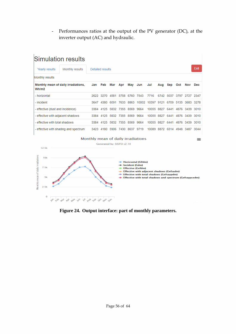
Page 56 of 64
- Performances ratios at the output of the PV generator (DC), at the inverter output (AC) and hydraulic.
Figure 24. Output interface: part of monthly parameters.

Page 57 of 64
3-4 Detailed Results This tab allows the visualization of additional and detailed data divided
in 4 main groups:
- Irradiation on the horizontal surface
- Irradiation on the inclined surface
- Electric energies
- Pumping
Monthly mean values (12 values), monthly values (12 values), and daily values (365 values) are available.
3-5 Generate technical report This tab will be available soon and will allow the generation of a pdf
technical report.
3-6 New simulation A new simulation can be performed because the input tab is still
available. This way, one can redefine some of the parameters and adjust the simulation results to an optimized case.

Page 58 of 64
4 ANNEX: Simulation variables
4-1 Introduction This annex includes a detailed list of the variables that can be selected in
Yearly, Monthly and Detailed Results to be analysed.
4-2 List of simulation variables
4-2-1 Meteorological variables - Radiation on the horizontal surface
Table 30. Horizontal irradiances.
Variable Unit Definition G0 W·m-2 Global B0 “ Beam D0 “ Diffuse
4-2-2 Meteorological variables - Radiation on the inclined surface
Table 31. Irradiances on the inclined surface.
Variable Unit Definition G W·m-2 Global B “ Beam D “ Diffuse R “ Reflected
Gef “ Global effective (includes dust and incidence effects) Bef “ Beam effective

Page 59 of 64
Def “ Diffuse effective Ref “ Reflected effective
Gefsa “ Global effective plus adjacent shading Befsa “ Beam effective plus adjacent shading Defsa “ Diffuse effective plus adjacent shading
Gefsayp “ Global effective plus adjacent and back shading Befsayp “ Beam effective plus adjacent and back shading Defsayp “ Diffuse effective plus adjacent and back shading
Gefsaypce “ Global effective plus adjacent and back shading, and spectral correction
Befsaypce “ Beam effective plus adjacent and back shading, and spectral correction
Defsaypce “ Diffuse effective plus adjacent and back shading, and spectral correction
Refce “ Reflected effective and spectral correction
4-2-3 Meteorological variables - Daily, monthly and yearly irradiations
Daily, monthly and yearly irradiations are indicated, respectively, with the suffixes “d”, “m” and “a” after the irradiance name.
For example:
G0d is the daily horizontal irradiation, Wh·m-2 (365 values).
G0m is the monthly horizontal irradiation, Wh·m-2 (12 values).
G0dm is the monthly mean of daily horizontal irradiation, Wh·m-2 (12 values).
G0a is the yearly horizontal irradiation, Wh·m-2 (1 value).
4-2-4 PV system - Powers Table 32. PV system powers.
Variable Unit Definition
PDCSP kW/kWp Nominal DC power
PDCPP “ Less mismatch losses, power below the nominal one, and other effects (all these losses are included in the
PRVPN parameter of PVGEN)
PDCPT “ Less temperature losses
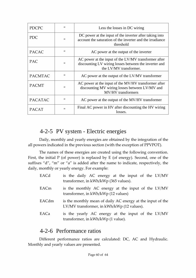
Page 60 of 64
PDCPC “ Less the losses in DC wiring
PDC “ DC power at the input of the inverter after taking into
account the saturation of the inverter and the irradiance threshold
PACAC “ AC power at the output of the inverter
PAC “ AC power at the input of the LV/MV transformer after discounting LV wiring losses between the inverter and
the LV/MV transformer.
PACMTAC “ AC power at the output of the LV/MV transformer
PACMT “ AC power at the input of the MV/HV transformer after
discounting MV wiring losses between LV/MV and MV/HV transformers
PACATAC “ AC power at the output of the MV/HV transformer
PACAT “ Final AC power in HV after discounting the HV wiring losses.
4-2-5 PV system - Electric energies Daily, monthly and yearly energies are obtained by the integration of the
all powers indicated in the previous section (with the exception of PPVPOT).
The names of these energies are created using the following convention. First, the initial P (of power) is replaced by E (of energy). Second, one of the suffixes “d”, “m” or “a” is added after the name to indicate, respectively, the daily, monthly or yearly energy. For example:
EACd is the daily AC energy at the input of the LV/MV transformer, in kWh/kWp (365 values).
EACm is the monthly AC energy at the input of the LV/MV transformer, in kWh/kWp (12 values)
EACdm is the monthly mean of daily AC energy at the input of the LV/MV transformer, in kWh/kWp (12 values).
EACa is the yearly AC energy at the input of the LV/MV transformer, in kWh/kWp (1 value).
4-2-6 Performance ratios Different performance ratios are calculated: DC, AC and Hydraulic.
Monthly and yearly values are presented.

Page 61 of 64
4-2-7 Other performance indices The following performance indices are also calculated, but only on yearly
basis.
Table 33. Other performance indices.
Variable Unit Efficiency of
LCa % Capture losses, relative to Yr
LSa % System losses, relative to Yr
4-2-8 PV pumping system - Instantaneous values Table 34. Hydraulic variables.
Variable Unit Definition
H m Head
Q m3/h Flow rate
FLOW (m3/h)/kWp Normalised flow rate
Table 35. Pumping powers.
Variable Unit Definition
P1 kW/kWp Input power to the motor
P2 “ Shaft power (mechanical output power of the motor)
PH “ Hydraulic power
4-2-9 PV pumping system - Daily, monthly and yearly parameters
Daily, monthly and yearly energies are obtained by the integration of the all powers indicated in the previous section.

Page 62 of 64
The names of the energies are created replacing the initial P (of power) by E (of energy) and adding the suffixes “d”, “m” or “a”, respectively, to indicate daily, monthly or yearly energy. For example:
E1d is the daily PV energy, in kWh/kWp (365 values).
E1m is the monthly PV energy, in kWh/kWp (12 values).
E1dm is the monthly mean of daily PV energy, in kWh/kWp (12 values).
E1a is the daily PV energy, in kWh/kWp (1 value).

Page 63 of 64
5 References
[1] Market uptake of an innovative irrigation Solution based on LOW WATer-Energy consumption (MASLOWATEN). Contract 640771.
[2] PVGIS database: http://re.jrc.ec.europa.eu/pvgis/ [3] Page J.K. The estimation of monthly mean values of daily total shortwave
radiation on vertical and inclined surfaces from sunshine records for latitudes 40°N-40°S. Proceedings U.N. Conference on New Sources of Energy 1961, 378-390.
[4] Erbs, D.G., S.A. Klein, and J.A. Duffie. “Estimation of the Diffuse Radiation Fraction for Hourly, Daily and Monthly-average Global Radiation.” Solar Energy 28, no. 4 (1982): 293–302.
[5] Macagnan, M.H., E. Lorenzo, and C. Jimenez. “Solar radiation in Madrid” International Journal of Solar Energy 16, no. 1 (May 1994): 1–14.
[6] Collares-Pereira, Manuel, and Ari Rabl. “The Average Distribution of Solar Radiation-correlations Between Diffuse and Hemispherical and Between Daily and Hourly Insolation Values.” Solar Energy 22, no. 2 (1979): 155–164.
[7] Lorenzo, Eduardo. “Energy Collected and Delivered by PV Modules.” In Handbook of Photovoltaic Science and Engineering, edited by Antonio Luque and Steven Hegedus, 984–1042. John Wiley & Sons, Ltd, 2011.
[8] Ross R. G. Interface Design considerations for terrestrial solar cell modules. Proceedings of the 12th IEEE Photovoltaic Specialists Conference – 1976 Baton Rouge, Louisiana, A78-10902 01-44, pp. 801-806.
[9] Martínez-Moreno, F., E. Lorenzo, J. Muñoz, and R. Moretón. “On the Testing of Large PV Arrays.” Progress in Photovoltaics: Research and Applications 20, no. 1 (2012): 100–105.
[10] E. Skoplaki, J. A. Palyvos. Operating temperature of photovoltaic modules: A survey of pertinent correlations. Renewable Energy, Volume 34, Issue 1, January 2009, Pages 23-29.
[11] Lorenzo, E., L. Narvarte, and J. Muñoz. “Tracking and Back-tracking.” Progress in Photovoltaics: Research and Applications 19, no. 6 (2011): 747–753.

Page 64 of 64
[12] M. Jantsch, H. Schmidt, J. Schmid. Results of the concerted action on power conditioning and control. 11th European Photovoltaic Solar Energy Conference 1992: 1589-1592.
[13] Muñoz, J., Martínez-Moreno, F. and Lorenzo, E. (2011), On-site characterisation and energy efficiency of grid-connected PV inverters. Prog. Photovolt: Res. Appl., 19: 192–201.
[14] Chapman, Stephen J. Electric Machinery Fundamentals. 5th edition, McGraw-Hill, 2011.
[15] J. Muñoz, J. Carrillo, F. Martínez-Moreno, L. Carrasco and L. Narvarte, "Modeling and simulation of large PV pumping systems," in Proceedings of the 31th European Photovoltaic Solar Energy Conference and Exhibition, Hamburg, 2015.
[16] Narvarte, L., and E. Lorenzo. “Tracking and Ground Cover Ratio.” Progress in Photovoltaics: Research and Applications 16, no. 8 (2008): 703–714.
[17] Hay, J. E., and McKat D.C.. “Estimating Solar Irradiance on Inclined Surfaces: A Review and Assessment of Methodologies.” International Journal of Solar Energy 3, no. 4–5 (1985):203–240.
[18] Perez, Richard, Robert Seals, Pierre Ineichen, Ronald Stewart, and David Menicucci. “A New Simplified Version of the Perez Diffuse Irradiance Model for Tilted Surfaces.” Solar Energy 39, no. 3 (1987): 221–231.
[19] Martin, N., and J.M. Ruiz. “Calculation of the PV Modules Angular Losses Under Field Conditions by Means of an Analytical Model.” Solar Energy Materials and Solar Cells 70, no. 1 (December 2001): 25–38.
[20] Martínez-Moreno, F., J. Muñoz, and E. Lorenzo. “Experimental Model to Estimate Shading Losses on PV Arrays.” Solar Energy Materials and Solar Cells 94, no. 12 (December 2010): 2298–2303.
[21] Martín, N., and J. M. Ruiz. “A New Method for the Spectral Characterisation of PV Modules.” Progress in Photovoltaics: Research and Applications 7, no. 4 (1999): 299–310.
[22] M. Iqbal. An Introduction to Solar Radiation, Chapter 9. Academic Press, (1983).