site properties inferred from delaney park downhole...

SITE PROPERTIES INFERRED FROM DELANEY PARK 1

DOWNHOLE ARRAY IN ANCHORAGE, ALASKA 2

Erol Kalkan1, Hasan S. Ulusoy2, Weiping Wen3, Jon. P. B Fletcher1, Fei Wang4 and Nori 3

Nakata5 4

1Earthquake Science Center, U. S. Geological Survey, CA, 94025, USA 5 2Consulting Engineer, Palo Alto, CA, USA 6 3 Key Lab of Structures Dynamic Behavior and Control of the Ministry of Education, Harbin Institute of 7

Technology, Harbin, 150090, China 8 4Earthquake Administration of Beijing Municipality, Beijing, China 9 5Department of Geophysics, Stanford University, CA, 94305, USA 10

11

12

13

14

15

16

17

18

19

20

Peer Review DISCLAIMER: This draft manuscript is distributed solely for purposes of scientific 21

peer review. Its content is deliberative and pre-decisional, so it must not be disclosed or released 22

by reviewers. Because the manuscript has not yet been approved for publication by the U.S. 23

Geological Survey (USGS), it does not represent any official USGS finding or policy. 24

“Bulletin of Seismological Society of America” v. 3.7

Kalkan et al. (2016) IP-062635 1

ABSTRACT 25

Waveforms recorded at various borehole depths were used to quantify site properties 26

including predominant frequencies, shear-wave velocity profile, shear modulus, soil damping 27

and site amplification at Delaney Park in downtown Anchorage, Alaska. The waveforms 28

recorded by surface and six boreholes (up to 61 m depth) three-component accelerometers were 29

compiled from ten earthquakes that occurred from 2006 to 2013 with moment magnitudes 30

between 4.5 and 5.4 over a range of azimuths at epicentral distances of 11 to 162 km. The 31

deconvolution of the waveforms at various borehole depths on horizontal sensors with respect to 32

the corresponding waveform at the surface provides upward (incident) and downward (reflected) 33

traveling waves within the soil layers. The simplicity and similarity of the deconvolved 34

waveforms from different earthquakes suggest that a one-dimensional shear-beam model is 35

accurate enough to quantify the soil properties. The shear-wave velocities determined from 36

different earthquakes are consistent, and agree well with the logging data; the deconvolution 37

interferometry predicts the shear-wave velocities within 15% of the in-situ measurements. The 38

site amplifications based on surface-to-downhole traditional spectral ratio (SSR), response 39

spectral ratio (RSR), cross-spectral ratio (cSSR), and horizontal-to-vertical spectral ratio (HVSR) 40

of the surface recordings were also evaluated. Based on cSSR, the site amplification was 41

computed as 3.5 at 1.5 Hz (0.67 s), close to the predominant period of the soil column. This 42

amplification agrees well with the average amplification reported in and around Anchorage by 43

previous studies. 44

Keywords: Site amplification, downhole array, wave propagation, interferometry, 45

deconvolution, shear-wave velocity, spectral analysis, Bootlegger Cove formation. 46


Kalkan et al. (2016) IP-062635 2

INTRODUCTION 47

Anchorage, Alaska, lies within one of the most active tectonic environments, and thus has 48

been subjected to frequent seismic activity. The city is built on the edge of a deep sedimentary 49

basin at the foot of Chugach Mountain Range. The basin is over 1 km in thickness in the western 50

part of Anchorage, and reaches 7 km depth at a point about 150 km southwest of the city 51

(Hartman et al., 1974). Shear-wave velocities, measured at 36 sites (Nath et al., 1997) in the 52

basin, indicate that most of the city is on sediments that fall in National Earthquake Hazard 53

Reduction Program (NEHRP) site categories C (360 < VS30 < 760 m/s; VS30 = average shear-54

wave velocity of upper 30 m of crust) and D (180 < VS30 < 360 m/s) (Boore, 2004). The existence 55

of low-velocity sediments overlying metamorphic bedrock can produce strong seismic waves 56

(Borcherdt, 1970). The Great Alaskan earthquake (a.k.a. Prince William Sound earthquake) with 57

moment magnitude (M) 9.2 in March 27, 1964, damaged the city, creating extensive 58

liquefaction, landslides and subsidence as large as 3 m in the downtown area (Updike and 59

Carpenter, 1986; Lade et al., 1988), and moved much of coastal Alaska seaward at least 80 m due 60

to ground failures (Brocher et al., 2014). 61

In 2003, the U.S. Geological Survey’s (USGS) Advanced National Seismic System 62

established a seven-level downhole array of three-component accelerometers at Delaney Park in 63

downtown Anchorage in order to measure sediments response to earthquake shaking, and to 64

provide input wave-field data for soil-structure interaction studies of a nearby twenty-story steel 65

moment frame building (Atwood Building), also instrumented. Figure 1 shows the photo and 66

map view of this downhole array (henceforth denoted as DPK) and Atwood Building in the 67

background. The deepest downhole sensors are located at 61 m depth within the soil layer 68

corresponding to the engineering bedrock. 69


Kalkan et al. (2016) IP-062635 3

Since 2003, more than a dozen earthquakes with M4.5 and above have been recorded at the 70

DPK. These recordings provide an excellent opportunity to extract the site properties, and 71

compare them with those from the earlier studies. The waveforms used in this study are rich 72

enough in low-frequency content that the site amplifications can be computed at low frequencies. 73

First, we applied deconvolution interferometry to the waveforms from ten earthquakes in order to 74

compute shear-wave velocity profile, shear modulus and soil damping. The deconvolution 75

interferometry provides a simple model of wave propagation by considering correlation of 76

motions at different observation points (e.g., Aki, 1957; Claerbout, 1968; Trampert et al. 1993; 77

Lobkis and Weaver, 2001; Roux and Fink, 2003; Schuster et al., 2004; Bakulin and Calvert, 78

2006; Snieder et al., 2006). It also yields more repeatable and higher resolution wave-fields than 79

does cross-correlation interferometry (Nakata and Snieder, 2012; Wen and Kalkan, 2016). Our 80

approach is similar but we identified incident and reflected deconvolved waves and used time 81

reversal to determine the site properties. Although deconvolution and cross-correlation 82

interferometry are interrelated, we preferred the deconvolution interferometry for this study 83

because the effects of the external source have been removed in the latter approach (Snieder and 84

Safak, 2006; Rahmani and Todorovska, 2013). Second, we estimated predominant frequencies of 85

the DPK array by utilizing a frequency response function (FRF), and also by using the average 86

shear-wave velocity of the soil column. Third, the site amplification based on the surface-to-87

downhole traditional spectral ratio (SSR), response spectral ratio (RSR), cross-spectral ratio 88

(cSSR), and horizontal-to-vertical spectral-ratio (HVRS) with surface recordings was evaluated 89

and compared. 90

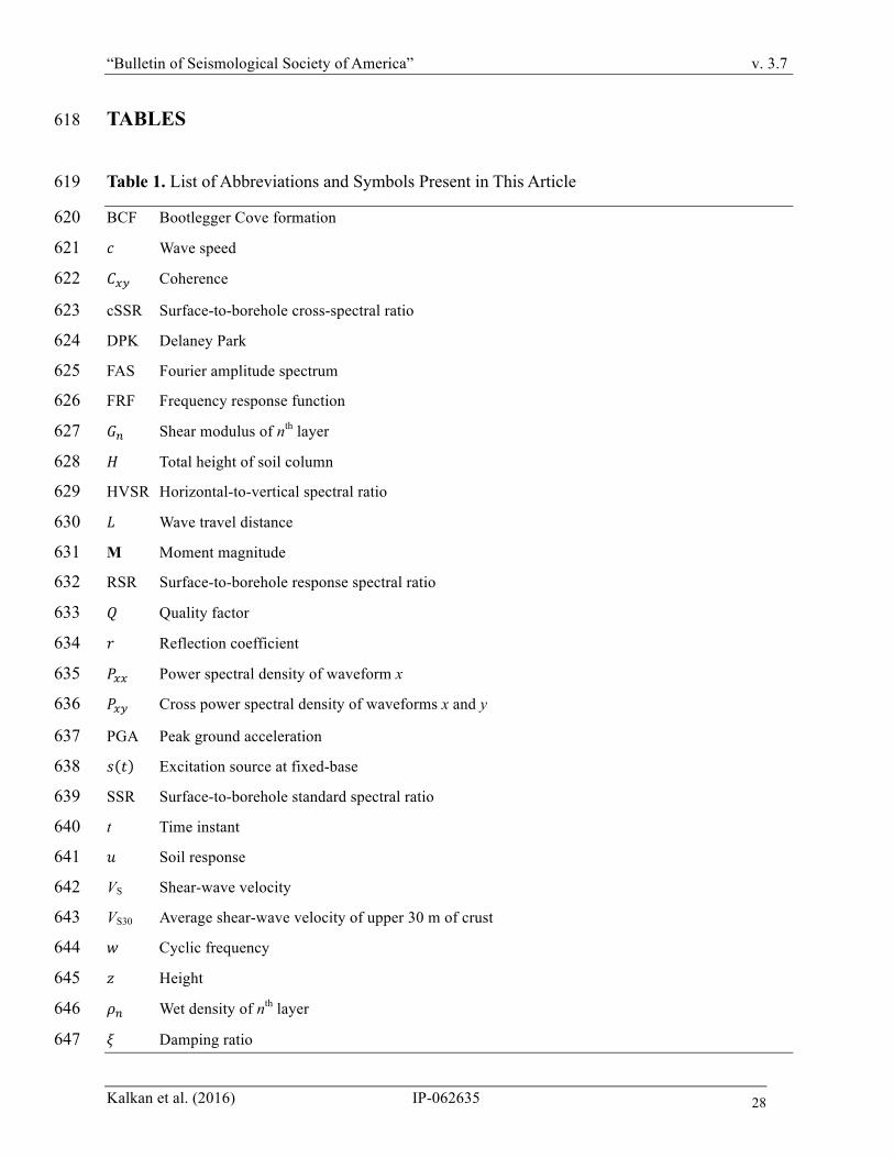
The complete list of abbreviations and symbols used throughout this article is given in Table 91

1. 92


Kalkan et al. (2016) IP-062635 4

TECTONIC SETTING 93

The Anchorage area is located in the upper Cook Inlet region. Cook Inlet is situated in a 94

tectonic forearc basin that is bounded to the west by the Bruin Bay-Castle Mountain fault system 95

and to the east by the Border Ranges fault system including the Knik fault along the west front of 96

the Chugach Mountains as depicted in Figure 2 (Lade et al., 1988). Most of the regional 97

seismicity can be attributed to under-thrusting along the Benioff zone (within ~150 km of 98

Anchorage) of the plate boundary megathrust (Li et al., 2013). Large historical earthquakes have 99

ruptured much of the length of this megathrust (Wong et al., 2010). The Benioff zone (its contour 100

is shown by thick dashed line) dips to the northwest beneath the Cook Inlet region (Fogelman et 101

al., 1978). 102

Smart et al. (1996) suggests that the Paleogene strike slip along the Border Ranges fault was 103

transferred to dextral slip on the Castle Mountain fault through a complex fault array in the 104

Matanuska Valley and strike-slip duplex systems in the northern Chugach Mountains. There is 105

some evidence suggesting that both the Castle Mountain (Bruhn, 1979; Lahr et al., 1986) and 106

Border Ranges fault systems (Updike and Ulery, 1986) may be active, and capable of 107

propagating moderate size earthquakes. The Castle Mountain fault approaches to within about 40 108

km of the city. Each year earthquakes with moment magnitudes above 4.5 are felt in Anchorage 109

as a result of this tectonic setting. 110

THE SITE, INSTRUMENTATION AND EARTHQUAKE DATA 111

DPK array is located at north-west downtown Anchorage as shown in map view in Figure 1. 112

The geological section at the site consists of glacial outwash, overlying Bootlegger Cove 113


Kalkan et al. (2016) IP-062635 5

formation (BCF) and glacial till deposited in a late Pleistocene glaciomarine-glaciodeltaic 114

environment (14,000–18,000 years ago) (Ulery et al., 1983). The glacial outwash contains 115

gravel, sand and silt, commonly stratified, deposited by glacial melt water. This surficial mud 116

layer of soft estuarine silts overlays an approximately 35 m thick glacio-estuarine deposit of stiff 117

to hard clays with interbedded lenses of silt and sand. This glacio-estuarine material is known 118

locally as the BCF. Underlying the BCF is a glaciofluvial deposit from the early Naptowne 119

glaciation (Updike and Carpenter, 1986) consisting mainly of dense to very dense sands and 120

gravels with interbedded layers of hard clay (Finno and Zapata-Medina, 2014). The BCF (from 121

20-50 m depth) has major facies with highly variable physical properties (Updike and Ulery, 122

1986). Cone penetration test blow counts are down in the single digits at depths of over 30 m in 123

BCF, and shear-wave velocity diminishes with depth through this formation (Steidl, 2006). The 124

glacial till is composed of unsorted, nonstratified glacial drift consisting of clay, silt, sand and 125

boulders transported and deposited by glacial ice. The relatively thin (<12.5 m) glacial outwash 126

at the surface is locally underlain by sensitive facies of the BCF that could cause catastrophic 127

failures during earthquakes, as occurred during the 1964 great Alaska earthquake. The DPK array 128

has been deployed to sample the ground motions within this formation, as well as above and 129

below it (Figure 3). The deepest borehole sensor is located in a glacial till formation with VS > 130

900 m/s, corresponding to engineering bedrock. Due to lack of in-situ measurements at the DPK 131

site, the shear-wave velocity (VS) of soil column have been estimated by Nath et al. (1997) and 132

Yang et al. (2008) in Figure 4 from inversion of data at a nearby site, about 200 m away (U. 133

Dutta, oral commun., 2014). The VS increases initially within the glacial outwash at shallower 134

depths, and then decreases within the deeper BCF. 135

The DPK array consists of one surface and six borehole tri-axial accelerometers located at 136


Kalkan et al. (2016) IP-062635 6

4.6, 10.7, 18.3, 30.5, 45.4 and 61 m depth, and oriented to cardinal directions as marked in 137

Figure 3. These borehole depths do not correspond to the depth of the boundary of soil layers. 138

The accelerometers in boreholes (Episensors) are connected to four six-channels 24-bit data 139

loggers (Quanterra-330). More than a dozen earthquakes with M4.5 and above have been 140

recorded since the deployment of the DPK array. Ten earthquakes with M between 4.5 and 5.4 141

were identified for this study based on their proximity to the site and recordings’ intensity. The 142

distant earthquakes were discarded due to low signal-to-noise ratio of the waveforms. The events 143

selected are listed in Table 2 along with distance and epicenter. The event epicenters are depicted 144

on a regional map in Figure 5; also shown in this figure are known faults around the city. Most of 145

the events selected are 35–83 km deep, and 80% of records are considered as far-field since they 146

were recorded at epicentral distances larger than 20 km. All earthquake data have a sampling rate 147

of 200 samples-per-second with a minimum duration of 222 s, covering potential surface waves. 148

The 2012 M4.6 earthquake is the closest event with a peak ground acceleration (PGA) of 1.8% 149

g, recorded at epicentral distance of 10.8 km. The largest PGA of 3.1% g (see Figure 6) was 150

recorded during the 2010 M4.9 event at epicentral distance of 20.7 km. Figure 6 shows the 151

motions from glacial till amplify as they propagate within the BCF, and de-amplify within the 152

transition region to glacial outwash due to impedance contrast. 153

DECONVOLUTION INTERFEROMETRY 154

A one-dimensional shear-beam model provides useful information about soil response to 155

ground shaking (Iwan, 1997). For soil column with uniform mass and stiffness, the shear-wave 156

propagation can be expressed in the time domain as: 157


Kalkan et al. (2016) IP-062635 7

𝑢 𝑡, 𝑧 = 𝐴 𝑡, 𝑧 ∙ 𝑠 𝑡 −𝑧𝑐 + 𝐴 𝑡, 2𝐻 − 𝑧 ∙ 𝑠 𝑡 −

2𝐻 − 𝑧𝑐 + 158

𝑟 ∙ 𝐴 𝑡, 2𝐻 + 𝑧 ∙ 𝑠 𝑡 − /0123

+ 𝑟 ∙ 𝐴 𝑡, 4𝐻 − 𝑧 ∙ 𝑠 𝑡 − 50623

+ ⋯ (1) 159

where 𝑢(𝑡, 𝑧) is the soil response at height 𝑧(𝑧 = 0 at the bottom of the borehole) at time 𝑡, 160

𝑠 𝑡 is the excitation source at the fixed-base, 𝐻 is the total height, 𝑐 is the traveling shear-wave 161

speed, and 𝑟 is the reflection coefficient at 𝑧 = 0. 𝑟 was assumed to be zero for the borehole case. 162

The attenuation occurs during wave propagation in soil column when a wave travel over a 163

distance L, which is described by attenuation operator 𝐴(𝐿, 𝑡). For a constant 𝑄-model, this 164

attenuation operator in frequency domain is given by Aki and Richards (2002): 165

𝐴 𝑤, 𝐿 = exp(−𝜉 ∙ 𝑤 ∙ 𝐿/𝑐) (2) 166

where 𝑤 is the cyclic frequency defined as 2𝜋/𝑡 , 𝜉 is the viscous damping ratio [𝜉 =1/(2𝑄)]. 167

Equation (1) shows that the soil response is the summation of an infinite number of the 168

upward and downward traveling waves. The first term is the upward traveling wave, and the 169

second term represents the reflection of the first wave at the free end, and travels downward. 170

This wave reflects off the fixed-base and travels upward, which is the third term. The last term is 171

the reflection of the third wave at the free end, which travels downward. For the attenuation 172

model in Equation (2), the soil response in the frequency domain is expressed as: 173

𝑈 𝑤, 𝑧 = 𝑆 𝑤HIJK 𝑅I exp(𝑖 ∙ 𝑘 ∙ (2𝑛 ∙ 𝐻 + 𝑧)) ∙ exp(−𝜉 ∙ 𝑘 ∙ (2𝑛 ∙ 𝐻 + 𝑧)) +174

exp 𝑖 ∙ 𝑘 ∙ 2 𝑛 + 1 𝐻 − 𝑧 ∙ exp −𝜉 ∙ 𝑘 ∙ 2 𝑛 + 1 𝐻 − 𝑧 (3) 175

where 𝑘 = 𝑤/𝑐 is the wave number, 𝑖 is the imaginary unit. The deconvolution of the response at 176

height 𝑧 by the response at the free end (surface for soil) is defined in frequency domain by 177


Kalkan et al. (2016) IP-062635 8

𝐷 𝑤, 𝑧 = 𝑈 𝑤, 𝑧 /𝑈 𝑤,𝐻 (4) 178

By plugging equation (3) into equation (4), and making appropriate cancellations, 𝐷 𝑤, 𝑧 can be 179

obtained as 180

𝐷 𝑤, 𝑧 = R/exp(𝑖 ∙ 𝑘 ∙ (−𝐻 + 𝑧))𝑒𝑥𝑝(−𝜉 ∙ 𝑘 ∙ (−𝐻 + 𝑧)) + exp 𝑖 ∙ 𝑘 ∙ 𝐻 − 𝑧 exp −𝜉 ∙181

𝑘 ∙ 𝐻 − 𝑧 (5) 182

Equation (5) shows that the soil response at height 𝑧 deconvolved by the response at the surface 183

is the summation of the two attenuated waves traveling upward and downward. Waveform 184

deconvolution decouples the soil response from the excitation because this deconvolution is 185

independent of the excitation source and the reflection coefficient (Snieder and Safak, 2006; 186

Nakata et al., 2013). Hence, the soil properties can be estimated from the deconvolved 187

waveforms. 188

RESULTS 189

We applied deconvolution interferometry to the data from ten earthquakes listed in Table 2. 190

The soil responses 𝑈 𝑤, 𝑧 from six boreholes were deconvolved by the soil response measured 191

at the surface U(w,H). The deconvolution was based on the single component (east-west) of the 192

horizontal motions because both horizontal components of records produced similar results. 193

Figure 7 shows the waveforms in Figure 6 after deconvolution with the waves at the surface. Full 194

lengths of the waveforms, low-cut filtered by a 4th order acausal Butterworth filter with corner 195

frequency of 0.1 Hz, are used. 196

The deconvolved wave at the surface is a bandpass-filtered Dirac delta function (virtual 197

source), because any waveform deconvolved with itself, with white noise added, yields a Dirac 198


Kalkan et al. (2016) IP-062635 9

delta function (pulse) at t = 0 (see Equation (4) with z = H). The deconvolved waveforms at 199

borehole-2 through borehole-6 demonstrate a wave state of the borehole array. This wave state is 200

the response of different soil layers to the delta function at the surface. For early times, the pulse 201

travels downward in the soil column with a velocity equal to shear-wave velocity of soil layers, 202

and response is superposition of upward and downward traveling waves. At t = 0, the wave field 203

is non-zero only at the surface. For later times, however, the waveforms are governed by site 204

resonance that decays exponentially with time due to attenuation (intrinsic damping). 205

The deconvolved waves shown in Figure 7 contain energy in the acausal part (no phase 206

shift). For negative time, upward going and downward going waves are present that reflect at the 207

surface at t = 0. If the waveforms are deconvolved with the waveform at borehole-6, they will 208

not display acausal arrivals; because there is no physical source at the surface, while the 209

borehole-6 is being shaken by the earthquake. The shaking at the borehole-6 would act as an 210

external source. The causality properties of the deconvolved waveforms are therefore related to 211

the existence (or non-existence) of a physical source of the recorded waves (Snieder et al., 2006). 212

The deconvolved waves in Figure 7 do not show notable intrinsic damping, but some pulse 213

broadening is apparent. This is consistent with the soil-damping ratio computed (will be 214

described later in “Soil-damping Ratio”). 215

Shear-wave Velocity 216

The shear-wave velocity of the upward and downward traveling waves (𝑉W,I) for the nth layer 217

between two boreholes is derived based on the time lag 𝜏between deconvolved waveforms and 218

the distance following the ray theory, which ignores wave scattering, 𝑉W,I = ℎ/𝜏, where h is the 219

distance. The wave travel time (𝜏) associated with the first borehole at 4.6 m is discarded 220


Kalkan et al. (2016) IP-062635 10

because of the overlapping upward and downward waves at this level. In Figure 8a and Figure 221

8b, the arrival time and travel distance of the upward and downward traveling waves are 222

identified to compute the shear-wave velocity profiles based on the 2010 M4.9 earthquake 223

waveforms shown in Figure 6. The negative values are due to the upward traveling waves, and 224

the positive values are associated with the downward traveling waves. A straight line is fitted to 225

all data points in Figure 8b by least squares with the Levenberg-Marquardt method (Levenberg, 226

1944; Marquardt, 1963) to determine a single average shear-wave velocity for the upper 61 m of 227

the soil. Figure 8c depicts the shear-wave velocity of layersfor the upward and downward 228

traveling waves, and compares them with the logged data shown by horizontal bars; the 229

deconvolution results in shear-wave velocities within 15% of the logged data. Note that the term 230

“layer” used here does not necessarily refer to soil layers with distinct physical parameters but 231

the soil medium between tips of two boreholes where the accelerometers are located, which are 232

shown by dash lines in Figure 8c. 233

The same process is repeated for the remaining recordings from nine earthquakes, and Table 234

3 summarizes the shear-wave velocity of the soil layers for each event; also given at the last row 235

of this table are the average shear-wave velocities considering all events. The difference of 236

velocity for upward and downward traveling waves is due to reflection between soil layers, 237

which creates epistemic noise. The shear-wave velocities of the five layers estimated from 238

different earthquakes are very close to each other. Among all layers, the maximum discrepancy 239

between different events is 17%. The last column of Table 3 lists the average shear-wave velocity 240

for the upper 61 m of the soil column for each event computed according to the least square fit 241

shown in Figure 8b. The average shear-wave velocities from the ten earthquakes are practically 242

the same with a maximum discrepancy of 1.7%, indicating that site response remained linear-243


Kalkan et al. (2016) IP-062635 11

elastic between different events. 244

Soil Predominant Frequencies 245

For a homogenous isotropic soil medium with one-dimensional wave propagation model, the 246

predominant frequency (𝑓) of the soil column can be derived from the shear-wave velocity, 𝑓 =247

𝑉[/4𝐻 where 𝐻 is the total height of the soil column. The predominant frequency derived by this 248

simple equation for each earthquake is presented in Table 4. The average value of 𝑓 is 1.2 Hz 249

when all events are considered. For comparison, the predominant frequency of the soil is also 250

computed from the FRF, defined as the surface response compared to the input of the deepest 251

borehole following the initial work done by Borcherdt (1970) and then Joyner el al. (1976) for 252

the San Francisco Bay. The FRF is computed as 253

𝐻(𝑓) = 𝑃]] 𝑓 𝑃]^(𝑓) (6) 254

where 𝑃]] is the power spectral density of the soil response measured at the surface, and 𝑃]^ is 255

the cross power spectral density of the soil response measured at the surface and at the borehole-256

6. Note that Equation (6) is inverted compared to most uses of this method. Figure 10 plots the 257

computed FRFs from ten events. The peaks around 5 to 6 Hz appear only for two events; we 258

attributed these spurious peaks to limitation of the FRF method, and rejected them. The first 259

three frequencies in the FRFs are listed in Table 4. The relative difference between the largest 260

and lowest predominant frequencies is 12%. The relative differences between the largest and 261

lowest second and the third frequencies are 5.6% and 3.2%, respectively. Average value of site 262

fundamental frequency (first mode) from ten earthquakes is 1.44 Hz. For all earthquakes, the 263

predominant frequency derived from the average shear-wave velocity of the soil column is 17% 264

smaller than that computed from the FRF. This difference is expected because the frequency 265


Kalkan et al. (2016) IP-062635 12

derived from the average shear-wave velocity is based on the assumption that the soil column 266

has a uniform mass and stiffness. This assumption often yields smaller frequencies. The average 267

ratios of the second and third frequencies to the predominant frequency are 2.8 and 4.8, 268

respectively while the corresponding analytical ratios are 3 and 5 for uniform soil column. 269

Site Amplification 270

Site amplification refers to the increase in amplitude of seismic waves as they propagate 271

through soft soil layers; this increase is the result of impedance contrast (impedance = density of 272

soil x VS) between different layers (Safak, 2001). A number of empirical site amplification 273

studies have been published for the Anchorage area (e.g., Nath et al., 2002; Martirosyan et al., 274

2002; Dutta et al., 2003). The last two studies computed site response at the basin stations 275

relative to a reference site in the nearby Chugach Mountains. All of the studies focused on site 276

response within the 0.5 to 11 Hz range, and all of the studies found significant frequency-277

dependent site amplifications on the sediments beneath the city. The largest site amplifications on 278

average were reported on the lower-velocity NEHRP class D sites, with average amplifications 279

around 3 at low frequencies (0.5–2.5 Hz) and around 1.5 at higher frequencies (3.0–7.0 Hz). 280

Safak (2001) provides a review of various methods to estimate site amplifications. In this 281

study, the site amplification is calculated with the following four different methods: (i) surface-282

to-borehole standard spectral ratio (SSR); (ii) surface-to-borehole cross-spectral ratio (cSSR); 283

(iii) horizontal-to-vertical spectral ratio (HVSR); and (iv) surface-to-borehole response spectral 284

ratio (RSR). 285

The SSR is the ratio of the Fourier spectra of the site recording to those of the reference-site 286

recording. The deepest borehole in this study is selected as a reference because it is embedded to 287


Kalkan et al. (2016) IP-062635 13

the engineering bedrock (glacial till). The borehole recording is influenced by the downward 288

waves reflected by the soil layers above, and the destructive interference among these waves 289

may cause unexpected peaks in the spectral ratios (Shearer and Orcutt, 1987; Steidl et al., 1996). 290

When shallow borehole data are used as reference for estimating amplification at the surface, the 291

potential maximum in the borehole spectrum would produce peaks in the spectral ratios that 292

could be miscalculated as site-response peaks. Steidl et al. (1996) suggests that coherence 293

estimate 𝐶]^ 𝑓 between the surface and borehole-recorded signals can be used to identify the 294

destructive interference effects that manifest as artificial peaks in the surface-to-borehole transfer 295

function. These artificial peaks correspond to the sinks in the coherence estimate. 296

In order to eliminate the effects of the destructive interference on site amplification, we 297

computed the cSSR, which is the product of the spectral ratio and the coherence function (Safak, 298

1997), to estimate the site amplification (Assimaki et al., 2008). The coherence 𝐶]^ 𝑓 of the 299

surface recording and borehole recording is computed as: 300

𝐶]^ 𝑓 = ab(c)d

aa(c) bb(c). (7)301

𝐶]^ 𝑓 ranges between zero and one, and it is used to assess the effects of noise in the 302

waveform. Frequency ranges in the transfer function that are dominated by noise (typically high 303

frequencies) demonstrate low coherence. At frequencies where sinks are observed in the 304

coherence estimate, the resulting cross-spectral estimate of the transfer function is expected to 305

deviate from the traditional spectral ratio, indicating the occurrence of destructive interference 306

phenomena. Such phenomena (incoherence) can be due to noise or to natural physical processes 307

such as wave passage, scattering and extended source effects (Zerva, 2009). 308

The HVSR is defined as the Fourier spectral ratio between the horizontal and vertical 309


Kalkan et al. (2016) IP-062635 14

recordings (Nakamura, 1989). It is widely used to estimate the fundamental resonance mode at a 310

site. The Fourier spectra of the horizontal recording are estimated by the root mean square of the 311

Fourier spectra of two horizontal components (Martirosyan et al., 2002). HVSR of earthquake 312

motions have also been used to identify the velocity profiles (Arai and Tokimatsu, 2004). A 313

thorough review of the HVSR implementation can be found in Kudo et al. (2004). Studies 314

showed that estimates of the frequency of the predominant peak from HVSR are similar to that 315

obtained with traditional spectral ratios; however, the absolute level of site amplification does 316

not correlate with the amplification obtained from more conventional methods (Lachet and Bard, 317

1994; Field and Jacob, 1995; Field, 1996; Lachet et al., 1996). Thus, HVSR is generally used to 318

analyze the fundamental resonance peaks but not to determine precisely the amplification levels 319

(Bonilla et al., 1997; Riepl et al., 1998; Parolai and Richwalski, 2004). 320

Finally, the RSR, defined as the ratio of 5% damped pseudo-spectral acceleration response 321

spectrum on surface to those on the deepest borehole, was used (Kitagawa et al., 1992). Pseudo-322

spectral acceleration response spectra and their ratios are much smoother functions of frequency 323

than the standard spectral ratios because the damped single-degree-of-freedom system acts as a 324

narrow-band filter. 325

The ratio of the Fourier amplitude spectrum (FAS) of two noisy records is very sensitive to 326

noise, and would have unrealistically high amplitudes if no smoothing were performed on the 327

FAS prior to taking the ratio. Thus, we applied a moving average filter with a length of 2 s (0.5 328

Hz) for smoothing in computing the RSR, cSSR and HVSR. 329

For each of these four methods, site amplifications at different frequencies were computed 330

and averaged across the ensemble of recordings considering all events. Figure 11 plots the mean 331

estimates. Note that the DPK array site has a shallow soft layer in the near surface with relatively 332


Kalkan et al. (2016) IP-062635 15

constant shear-wave velocity (295 m/s; NEHRP site category D) due to presence of BCF 333

overlying a relatively homogeneous stiff formation with strong impedance contrast at 50 m depth 334

(NEHRP site category B). In Figure 11, the values on the horizontal axis are the reciprocals of 335

the periods for the RSR. For each method, three obvious peaks can be seen at three frequency 336

ranges (1.1-1.5 Hz), (4.0-4.4 Hz) and (6.8-7.2 Hz), respectively. These peaks correspond to the 337

predominant frequencies for the first three modes as shown in Figure 10. The SSR method 338

produced the greater site amplification estimates than the cSSR and RSR methods with the 339

exception of HVSR method at low frequencies. Although the frequencies of the predominant 340

peaks from HVSR are similar, the absolute level of site amplification does not correlate well 341

with the amplification estimated from other methods. The SSR method predicts the maximum 342

site amplification as 5.3. This method is the least reliable because it is very sensitive to the noise 343

level in the waveforms, thus it is not appropriate for downhole recordings. 344

The maximum site amplification of 4.2 is predicted by the RSR method; this method is 345

applicable at low frequencies (e.g., less than 4 Hz), but not for high frequencies. The cSSR 346

method resulted in maximum site amplification as large as 3.5 at low frequencies close to the 347

first-mode frequency shown in Figure 10. 348

The average coherence estimates of the surface and the deepest borehole recordings are also 349

presented in Figure 11. Based on the equivalent homogeneous medium approach (Steidl et al., 350

1996), the first mode frequency at which destructive interference is expected to occur is 351

estimated as 1.2 Hz, which is also indicated in Figure 11 with the solid line arrow. Clearly, the 352

destructive interference phenomena is not strictly materialized, which may due to the variation of 353

the shear-wave velocity among different soil layers as can be seen in Figure 8c. However, the 354

dashed line with arrows in Figure 11 indicate that peak site amplification predicted by SSR 355


Kalkan et al. (2016) IP-062635 16

method generally corresponds to the sinks of coherence estimates. This phenomenon means that 356

the cSSR method can predict site amplification at low frequencies more reliably by removing the 357

potential destructive interference. 358

Soil-damping Ratio 359

During wave propagation, the energy loss induced by soil damping can be represented by the 360

following attenuation equation (Aki and Richards, 2002): 361

𝐴[ 𝑓 = 𝑒6e∙c∙f/g (8) 362

where 𝐴[ 𝑓 is the reduction in the amplitude of a sinusoidal wave of frequency 𝑓 when it 363

travels a distance of travel time 𝜏. The damping ratio 𝜉 is defined by the quality factor 𝑄 (𝜉 =364

1/2𝑄). 365

In order to evaluate the dynamic damping in structures, previous studies (Snieder and Safak, 366

2006; Prieto et al., 2010; Newton and Snieder, 2012; Nakata et al., 2013) used the equation (8) in 367

conjunction with deconvolved waves. We adapted the same approach for evaluating the soil 368

dynamic damping. First, the recordings at different soil layers were deconvolved with the 369

recordings at the deepest borehole, and then, the deconvolved waves were bandpass filtered by a 370

4th order Butterworth filter with cutoff frequencies of 0.5 and 2 Hz. These corner frequencies 371

were selected to extract the fundamental mode, and filtered out high and low frequencies. The 372

natural logarithm of the envelope of the bandpass-filtered waveforms corresponding to the M4.9 373

event is shown in Figure 11 by dashed lines. In order to separate the curves at different borehole 374

depths, the natural logarithm of the envelope is added with the number of 50 minus the depth of 375

the borehole (the depth is 0 at the surface). According to the equation (8), the slope of the curves 376

in Figure 11 depends on the attenuation of the waves, thus the offset has no influence on the 377


Kalkan et al. (2016) IP-062635 17

results. The slopes of the curves, which are similar at different layers, were computed by least-378

square fit between 0.5 s and 5.0 s (shown by solid lines). The slope of the solid line is equal to 379

−π𝑓/𝑄. The mean slope at different layers (which is quite consistent at different depths), and the 380

first mode frequencies in Table 4 were used to compute the 𝑄 and 𝜉. Table 5 summarizes the 381

resultant 𝑄 and 𝜉 for all events. The results are stable between different events with a coefficient 382

of variance of 0.16 for 𝑄. The average soil dynamic damping for the DPK array was found to be 383

4.5%. 384

Shear Modulus 385

In homogeneous and isotropic media, the velocity of a shear wave is controlled by the shear 386

modulus 𝐺I, which defines the magnitude of the shear stress that soil can sustain—an important 387

parameter for geotechnical engineering. The shear modulus 𝐺I for the nth soil layer is 388

𝐺I = 𝜌I ∙ 𝑉W,I/ (9) 389

where 𝜌Iis the density of the nth layer. A wet density of 1.96 g/cm3 was assigned to the BCF 390

(from 20-50 m depth) based on measurements of ten soil samples (Lade et al., 1988). The site at 391

which the undisturbed samples of the BCF were collected was found to be geologically typical of 392

the 60 city blocks that form the metropolitan "core area" of Anchorage including the DPK array. 393

Using equation (9) and shear-wave velocity values in Table 3, the shear modulus of the BCF at 394

the DPK array was found to be between 125 and 170.9 MPa. 395

CONCLUSIONS 396

In this study, we investigated the linear-elastic properties of the sediment layers in particular 397

the Bootlegger Cove formation (BCF) at Delaney Park (DPK) downhole array in downtown 398


Kalkan et al. (2016) IP-062635 18

Anchorage Alaska. BCF is a soft formation thought to be responsible for much of the 399

liquefaction damage during the 1964 M9.2 great Alaska earthquake. The waveforms recorded 400

from ten earthquakes were analyzed using deconvolution interferometry. The waveforms at 401

various depths were deconvolved by the waveforms recorded at the surface in order to identify 402

predominant frequencies, shear-wave velocity profile, shear modulus and soil dynamic damping. 403

To quantify the site amplification, surface-to-downhole traditional spectral ratio (SSR), response 404

spectral ratio (RSR), cross-spectral ratio (cSSR), and horizontal-to-vertical spectral ratio (HVSR) 405

were calculated. The site characteristic information obtained here can be used for soil-structure 406

interaction analysis of a nearby twenty-story steel-moment frame building (Atwood Building), 407

also instrumented. 408

The key findings of this study are as follows: 409

• The simplicity and similarity of the deconvolved waveforms from ten earthquakes 410

manifest that a one-dimensional shear-beam model is accurate enough to represent the 411

linear-elastic soil response at the DPK array under low intensity shaking. 412

• The deconvolution results in shear-wave velocities within 15% of the logged data. The 413

maximum discrepancy in shear-wave velocities on average of borehole levels between 414

different events is 17%. This suggests that the deconvolution interferometry is an 415

effective way to quantify the shear-wave velocity profile for geotechnical arrays lacking 416

in-situ measurements. 417

• The predominant soil frequency derived from the average shear-wave velocity is a crude 418

estimation that is less accurate than the estimation from frequency-response function 419

(FRF). For all earthquakes, the predominant frequency derived from the shear-wave 420

velocity of the soil column is on average 1.2 Hz, which is 17% smaller than 1.44 Hz 421


Kalkan et al. (2016) IP-062635 19

estimated from the FRFs. 422

• Despite high aleatoric variability in earthquake waveforms, which come from events 423

varying in size, distance and azimuth, the average shear-wave velocity of soil layers, and 424

the predominant frequency of the soil column are consistent; this indicates that the soil 425

properties remained linear-elastic during different earthquakes. 426

• Destructive interference phenomena were demonstrated to yield overestimation of site 427

response by means of the surface-to-borehole transfer function with the exception of 428

HVSR estimates in the low frequency range. The SSR method was found to be the least 429

reliable one as compared to cSSR, HVSR and RSR techniques because it is very sensitive 430

to the noise level, thus it is not a convenient method for computing site amplification 431

using downhole recordings. 432

• The RSR method was found to be applicable only for computing site amplification at low 433

frequencies (less than 4 Hz); its accuracy quickly diminishes at high frequencies. 434

• The HVSR method was generally found to represent the fundamental resonance peak but 435

not to determine precisely amplification levels, a conclusion also drawn by others. 436

• The cSSR method can predict site amplification more reliably by removing the potential 437

destructive interference, thus it is theoretically more accurate than the other methods. 438

cSSR resulted in average site amplification as large as 3.5 at low frequencies (1.1-1.5 Hz) 439

close to the first-mode frequency of the soil column. Other studies find on average that 440

the largest site amplifications are on the lower-velocity NEHRP class D (180 < VS30 < 360 441

m/s) sites in Anchorage, with average amplifications around 3.0 at low frequencies (0.5–442

2.5 Hz). We found site amplification 17% higher than the average amplification reported 443

by others. 444


Kalkan et al. (2016) IP-062635 20

DATA AND RESOURCES 445

Instruments of the National Strong Motion Network of USGS collected recordings used in 446

this study. The records are available from the first author upon request. Figure 3 is modified from 447

http://nees.ucsb.edu/facilities/atwood-building-anchorage (last accessed July, 2016). 448

ACKNOWLEDGMENTS 449

The authors thank Jack Boatwright, Mehran Rahmani, Brad Aagaard, Sebastiano D’Amico 450

and an anonymous reviewer for their reviews and providing valuable suggestions and comments, 451

which helped improving technical quality of this article. Special thanks are extended to Utpal 452

Dutta and Joey Yang for discussions on DPK array soil properties, Luke Blair for generating the 453

regional maps, Shahneam Reza for preparing the DPK array illustration, Jamie Steidl for making 454

the ground motion recordings available, Christopher Stephens for processing the waveforms, and 455

USGS’s National Strong Motion Network technicians, James Smith, Jonah Merritt and Jason De 456

Cristofaro for keeping the DPK array up and running. China Research Council provided the 457

financial support for Weiping Wen and Fei Wang. 458

REFERENCES 459

Aki, K. (1957). “Space and time spectra of stationary stochastic waves, with special reference to 460

microtremors”, Bull. Earthquake Res. Inst., Univ. of Tokyo, 35, 415–456. 461

Aki, K., and Richards, P.G. (2002). Quantitative seismology, University Science Books, Mill 462

Valley, California. 463

Arai, H. and Tokimatsu, K. (2004). “S-Wave Velocity Profiling by Inversion of Microtremor H/V 464


Kalkan et al. (2016) IP-062635 21

Spectrum”, Bull. Seismol. Soc. Am., 94(1): 53-63, doi: 10.1785/0120030028. 465

Assimaki, D., Li, W., Steidl, J.H. and Tsuda, K. (2008). “Site amplification and attenuation via 466

downhole array seismogram inversion: a comparative study of the 2003 Miyagi-Oki 467

aftershock sequence”, Bull. Seismol. Soc. Am., 98(1): 301-330. 468

Bakulin, A. and Calvert, R. (2006). “The virtual source method: Theory and case study”, 469

Geophysics, 71(4): S139–S150. 470

Bonilla, L.F., Steidl, J.H., Lindley, G.T., Tumarkin, A.G. and Archuleta, R.J. (1997). “Site 471

amplification in the San Fernando Valley, California: variability of site-effect estimation 472

using the S-wave, coda, and H/V methods”, Bull. Seismol. Soc. Am. 87, 710–730. 473

Boore, D.M. (2004). “Ground motion in Anchorage, Alaska, from the 2002 Denali fault 474

earthquake: Site response and displacement pulses”, Bull. Seism. Soc. Am., 94: S72-S84. 475

Borcherdt, R.D. (1970). “Effects of Local Geology on Ground Motion Near San Francisco Bay”, 476

Bull. Seism. Soc. Am., 60: 29–61. 477

Brocher, T.M., Filson, J.R., Fuis, G.S., Haeussler, P.J., Holzer, T.L., Plafker, G., and Blair, J.L. 478

(2014). The 1964 Great Alaska Earthquake and tsunamis—A modern perspective and 479

enduring legacies: U.S. Geological Survey Fact Sheet 2014–3018, 6 p., 480

http://dx.doi.org/10.3133/fs20143018. 481

Bruhn, R.L. (1979). Holocene displacements measured by trenching the Castle Mountain Fault 482

near Houston, Alaska: Alaska Division of Geological and Geophysical Surveys Geologic 483

Report 61, p. 1-4. 484

Claerbout, J.F. (1968). “Synthesis of a layered medium from its acoustic transmission response”, 485

Geophysics, 33(2): 264–269. 486


Kalkan et al. (2016) IP-062635 22

Dutta, U., Biswas, N., Martirosyan, A., Papageorgiou, A. and Kinoshita, S. (2003). “Estimation 487

of earthquake source parameters and site response in Anchorage, Alaska, from strong-motion 488

network data using generalized inversion method”, Phys. Earth Planet. Interiors, 137: 13–29. 489

Field, E.H. (1996). Spectral amplification in a sediment-filled valley exhibiting clear basin-edge 490

induced waves, Bull. Seismol. Soc. Am., 86: 991–1005. 491

Field, E.H. and Jacob, K.H. (1995). A comparison and test of various site response estimation 492

techniques, including three that are non-reference site dependent, Bull. Seismol. Soc. Am. 85: 493

1127–1143. 494

Finno, R.J. and Zapata-Medina, D.G. (2014). “Effects of Construction-Induced Stresses on 495

Dynamic Soil Parameters of Bootlegger Cove Clays“, J. Geotech. Geoenviron. Eng., 140(4): 496

04013051, doi: 10.1061/(ASCE)GT.1943- 5606.0001072. 497

Fogelman, K., Stephens, C., Lahr, J.C., Helton, S. and Allen, M. (1978). Catalog of earthquakes 498

in southern Alaska, October-December, 1977: U.S. Geological Survey Open-File Report 78-499

1097, 28 p. 500

Hartman, D.C., Pessel, G.H. and McGee, D.L. (1974). Stratigraphy of the Kenai group, Cook 501

Inlet, Alaska Div. Geol. Geophys. Surv. Open-File Rept. 49. Available at 502

http://www.dggs.alaska.gov/pubs/id/149 (last accessed November 2014). 503

Iwan, W.D. (1997). “Drift Spectrum: Measure of Demand for Earthquake Ground Motions”, 504

ASCE Journal of Structural Engineering, 123(4): 397-404. 505

Joyner, W.B., Warrick, R.E. and Oliver III, A.A. (1976). “Analysis of Seismograms from a 506

Downhole Array In Sediments Near San Francisco Bay”, Bull. Seism. Soc. Am., 66(3): 937-507

958. 508


Kalkan et al. (2016) IP-062635 23

Kitagawa Y, Okawa, I. and Kashima, T. (1992). “Observation and analyses of dense strong 509

motions at sites with different geological conditions in Sendai”, Proc. Int. Symp. on the 510

Effects of Surface Geology on Seismic Motions, vol. 1. Assoc. of Earthquake Disaster 511

Prevention; 25± 27:311±6. 512

Kudo, K., Sawada, Y. and Horike, M. (2004). “Current studies in Japan on H/V and phase 513

velocity dispersion of microtremors for site characterization”, Proc. 13th World Conference 514

on Earthquake Engineering, Paper No. 1144. 515

Lachet, C. and Bard, P.Y. (1994). “Numerical and theoretical investigations on the possibilities 516

and limitations of Nakamura’s technique”, J. Phys. Earth, 42: 377–397. 517

Lachet, C., Hatzfeld, D., Bard, P.Y., Theodulidis, N., Papaioannou, C. and Savvaidis, A. (1996). 518

“Site effects and microzonation in the city of Thessaloniki (Greece) comparison of different 519

approaches”, Bull. Seismol. Soc. Am. 86(6): 1692–1703. 520

Lade, P.V., Updike, R.G. and Cole, D.A. (1988). Cyclic Triaxial Tests of the Bootlegger Cove 521

Formation, Anchorage, Alaska: U.S. Geological Survey Bulletin 1825, 51 p. 522

Lahr, J.C., Page, R.A., Stephens, C.D. and Fogleman, K.A. (1986). “Sutton, Alaska, earthquake 523

of 1984-evidence for activity on the Talkeetna segment of the Castle Mountain fault system”, 524

Seismological Society of America Bulletin, 76: 967-983. 525

Levenberg, K. (1944). A method for the solution of certain non-linear problems in least squares, 526

Quart. J. Appl. Maths. II, no. 2, 164–168. 527

Li, J., Abers, G.A., Kim, Y. and Christensen, D. (2013). “Alaska megathrust 1: Seismicity 43 528

years after the great 1964 Alaska megathrust earthquake”, Journal of Geophysical Research: 529

Solid Earth, 118(9): 4861–4871. 530


Kalkan et al. (2016) IP-062635 24

Lobkis, O.I., and Weaver, R.L. (2001). “On the emergence of the Green’s function in the 531

correlations of a diffuse field”, J. Acoust. Soc. Am., 110: 3011–3017. 532

Marquardt, D. W. (1963). An Algorithm for Least-Squares Estimation of Nonlinear Parameters, 533

SIAM Journal on Applied Mathematics 11, no. 2, 431–441. 534

Martirosyan, A., Dutta, U., Biswas, N., Papageorgiou, A., and Combellick, R. (2002). 535

“Determination of site response in Anchorage, Alaska, on the basis of spectral ratio 536

methods”, Earthquake Spectra, 18(1): 85-104. 537

Nakata, N. and Snieder, R. (2012). “Estimating near-surface shear wave velocities in Japan by 538

applying seismic interferometry to KiK-net data”, Journal of Geophysical Research, 117: 539

B01308. 540

Nakamura, Y. (1989). A method for dynamic characteristics estimation of subsurface using 541

microtremor on the ground surface. QR Railway Technical Research Institute 30(1). 542

Nakata, N., Snieder, R., Kuroda, S., Ito, S., Aizawa, T. and Kunimi, T. (2013). “Monitoring a 543

building using deconvolution interferometry, I: Earthquake-data analysis”, Bull. Seismol. Soc. 544

Am. 103(3): 1662– 1678, doi: 10.1785/0120120291. 545

Nath, S. K., Chatterjee, D., Biswas, N. N., Dravinski, M., Cole, D.A., Papageorgiou, A., 546

Rodriguez, J.A., and Poran, C.J. (1997). “Correlation study of shear wave velocity in near 547

surface geological formations in Anchorage, Alaska”, Earthquake Spectra 13(1): 55-75. 548

Nath, S.K., Biswas, N.N., Dravinski, M.A. and Papageorgiou, A.S. (2002). “Determination of S-549

wave site response in Anchorage, Alaska in the 1–9 Hz frequency band”, Pure and applied 550

geophysics, 159(11-12): 2673-2698. 551

Newton, C. and Snieder, R. (2012). “Estimating intrinsic attenuation of a building using 552


Kalkan et al. (2016) IP-062635 25

deconvolution interferometry and time reversal”, Bull. Seismol. Soc. Am. 102(5): 2200-2208. 553

Parolai, S. and Richwalski, S. (2004). “The importance of converted waves in comparing H/V 554

and RSM site response estimates”, Bull. Seismol. Soc. Am. 94(1): 304–313. 555

Plafker, G., Gilpin, L.M. and Lahr, J.C. (1994). Neotectonic map of Alaska, in The Geology of 556

North America, vol. G-1, The geology of Alaska (G. Plafker and H.C. Berg, eds.), Geol. 557

Soc. Amer., Boulder, Colo., pp. 389-449. 558

Prieto, G.A., Lawrence, J.F., Chung, A.I. and Kohler, M.D. (2010). “Impulse response of civil 559

structures from ambient noise analysis”, Bull. Seismol. Soc. Am., 100(5A): 2322-2328. 560

Rahmani M. and Todorovska M.I. (2013). “1D system identification of buildings from 561

earthquake response by seismic interferometry with waveform inversion of impulse 562

responses – method and application to Millikan Library”, Soil Dynamics and Earthquake 563

Engrg. 47:157-174, doi: 10.1016/j.soildyn.2012.09.014. 564

Riepl, J., Bard, P.Y., Hatzfeld, D., Papaioannou, C. and Nechtschein, S. (1998). “Detailed 565

evaluation of site-response estimation methods across and along the sedimentary valley of 566

Volvi (EURO-SEISTEST)”, Bull. Seismol. Soc. Am., 88(2): 488–502. 567

Roux, P. and M. Fink (2003). “Green’s function estimation using secondary sources in a shallow 568

wave environment”, J. Acoust. Soc. Am., 113: 1406–1416. 569

Safak, E. (1997). “Models and methods to characterize site amplification from a pair of records”, 570

Earthquake Spectra, 13(1): 97-129. 571

Safak, E. (2001). “Local site effects and dynamic soil behavior”, Soil Dyn. and Eq. Eng., 21: 572

453-458. 573

Schuster, G.T., Yu, J., Sheng, J. and Rickett, J. (2004). “Interferometric daylight seismic 574


Kalkan et al. (2016) IP-062635 26

imaging”, Geophys. J. Int., 157: 838–852. 575

Shearer, P. M., and J. A. Orcutt (1987). “Surface and near-surface effects on seismic waves: 576

theory and borehole seismometer results”, Bull. Seismol. Soc. Am., 77: 1168–1196. 577

Smart, K.J., Pavlis, T.L., Sisson, V.B., Roeske, S.M. and Snee, L.W. (1996). “The Border 578

Ranges fault system in Glacier Bay National Park, Alaska: Evidence for major early 579

Cenozoic dextral strike-slip motion”, Canadian Journal of Earth Sciences 33(9): 1268-1282. 580

Snieder, R. and Safak, E. (2006). “Extracting the Building Response Using Seismic 581

Interferometry: Theory and Application to the Millikan Library in Pasadena, California”, 582

Bull. Seism. Soc. Am., 96(2): 586–598. 583

Snieder, R., Sheiman, J. and Calvert, R. (2006). “Equivalence of the virtual-source method and 584

wave-field deconvolution in seismic interferometry”, Physical Review, E 73, 066620. 585

Steidl, J.H. (2006). “Inventory of Existing Strong-Motion Geotechnical Arrays”, Proceedings of 586

the International Workshop for International Workshop for Site Selection, Installation, and 587

Operation of Geotechnical Strong-Motion Arrays Workshop 2: Guidelines for Installation, 588

Operation, and Data Archiving and Dissemination, La Jolla, California, Cosmos Publication 589

No. CP-2006/01 (http://www.cosmos-eq.org/publications/CP-2006-01.pdf). 590

Steidl, J.H., Tumarkin, A.G. and Archuleta, R.J. (1996). “What is a reference site?”, Bull. 591

Seismol. Soc. Am., 86: 1733–1748. 592

Trampert, J., Cara, M. and Frogneux, M. (1993). “SH propagator matrix and QS estimates from 593

borehole- and surface-recorded earthquake data”, Geophysical Journal International 594

112:290–299. 595

Ulery, C.A., Updike, R.G. and USGS Office of Earthquakes (1983). “Subsurface structure of the 596


Kalkan et al. (2016) IP-062635 27

cohesive facies of the Bootlegger Cove formation, southwest Anchorage: Alaska”, Division 597

of Geological & Geophysical Surveys Professional Report 84, 5 p., 3 sheets, scale 1:15,840. 598

Updike, R.G. and Carpenter, B.A. (1986). “Engineering Geology of the Government Hill Area, 599

Anchorage, Alaska”, U.S. Geol. Surv. Bull.,1588, 36 pp. 600

Updike, R.G. and Ulery, C.A. (1986). Engineering - geologic map of southwest Anchorage, 601

Alaska: Alaska Division of Geological & Geophysical Surveys Professional Report 89, 1 602

sheet, scale 1:15, 840. doi:10.14509/2270. 603

Yang, Z., Dutta, U., Xiong, F., Biswas, N. and Benz, H. (2008). “Seasonal frost effects on the 604

dynamic behavior of a twenty-story office building”, Cold Regions Sc. & Techn. 51:76-84. 605

Wen, W. and Kalkan, E. (2016). “Interferometric System Identification—An Application to a 606

Twenty-story Instrumented Building in Anchorage, Alaska”, Bull. Seismol. Soc. Am. (in-607

review). 608

Wong I., Dawson, T., Dober, M. and Hashash, Y. (2010). “Evaluating the seismic ha ni draz609

Anchorage, Alaska”, Proc. of the 9th U.S. National and 10th Canadian Conference on 610

Earthquake Engineering, July 25-29, Toronto, Ontario, Canada, paper no: 785. 611

Zerva, A (2009). Spatial variation of seismic ground motions: modeling and engineering 612

applications. CRC Press. ISBN ISBN-10: 0849399297; ISBN-13: 978-0849399299. 613

614

615

616

617


Kalkan et al. (2016) IP-062635 28

TABLES 618

Table 1. List of Abbreviations and Symbols Present in This Article 619

BCF Bootlegger Cove formation 620

𝑐 Wave speed 621

𝐶]^ Coherence 622

cSSR Surface-to-borehole cross-spectral ratio 623

DPK Delaney Park 624

FAS Fourier amplitude spectrum 625

FRF Frequency response function 626

𝐺I Shear modulus of nth layer 627

𝐻 Total height of soil column 628

HVSR Horizontal-to-vertical spectral ratio 629

𝐿 Wave travel distance 630

M Moment magnitude 631

RSR Surface-to-borehole response spectral ratio 632

𝑄 Quality factor 633

𝑟 Reflection coefficient 634

𝑃]] Power spectral density of waveform x 635

𝑃]^ Cross power spectral density of waveforms x and y 636

PGA Peak ground acceleration 637

𝑠 𝑡 Excitation source at fixed-base 638

SSR Surface-to-borehole standard spectral ratio 639

t Time instant 640

𝑢 Soil response 641

VS Shear-wave velocity 642

VS30 Average shear-wave velocity of upper 30 m of crust 643

𝑤 Cyclic frequency 644

𝑧 Height 645

𝜌I Wet density of nth layer 646

𝜉 Damping ratio 647


Kalkan et al. (2016) IP-062635 29

𝜏 Wave travel time 648

649

Table 2. Origin Times, Magnitudes, Epicenters of Local and Regional Earthquakes Recorded by 650 The Delaney Park Borehole Array in Anchorage Alaska between 2006 and 2013 (See 651 “Data and Resources”) 652

Event No.

Origin time (UTC) (y-m-d)

Moment Magnitude

Epicenter Coordinates Latitude(°) Longitude(°)

Depth (km)

Epicentral Distance

(km)

Peak Acceleration

(cm/s2)

1 2013-03-13 5.4 62.559 -151.071 83.6 162.0 1.07

2 2012-05-16 4.6 61.118 -149.926 61.7 10.8 17.66

3 2011-06-16 5.1 60.765 -151.076 58.9 81.1 7.78

4 2010-09-20 4.9 61.115 -150.219 45.4 20.7 30.53

5 2010-07-08 4.8 61.805 -150.505 14.9 73.5 6.57

6 2010-04-07 4.6 61.580 -149.652 35.3 42.7 3.62

7 2009-08-19 5.1 61.228 -150.858 66.4 51.7 5.44

8 2009-06-22 5.4 61.939 -150.704 64.6 91.5 11.64

9 2006-09-06 4.5 61.621 -149.930 40.7 45.4 2.94

10 2006-07-27 4.7 61.155 -149.678 36.0 13.3 13.86

The earthquakes are numbered sequentially according to their origin times. Peak acceleration is the observed 653 absolute maximum amplitude of the waveforms from the accelerometers at the surface level 654 655 656 657 658 659 660 661 662 663 664 665 666 667 668 669 670


Kalkan et al. (2016) IP-062635 30

Table 3. Average Shear-wave Velocity of Soil Layers and Soil Column Identified based on 671 Upward and Downward Traveling Waves; Unit = m/s 672

Event No.

Layer 1

(0 - 10.7 m)

Layer 2

(10.7 - 18.3 m)

Layer 3

(18.3 - 30.5 m)

Layer 4

(30.5 - 45.4 m)

Layer 5

(45.4 - 61 m)

Average shear-wave

velocity of soil column

(up) (down) (up) (down) (up) (down) (up) (down) (up) (down)

1 305.7 305.7 253.3 253.3 244.0 244.0 270.9 298.0 780.0 624.0 295

2 267.5 267.5 304.0 253.3 221.8 271.1 298.0 298.0 780.0 624.0 293

3 267.5 267.5 253.3 304.0 271.1 244.0 270.9 298.0 780.0 624.0 293

4 305.7 305.7 217.1 253.3 271.1 244.0 270.9 298.0 780.0 624.0 294

5 267.5 305.7 304.0 253.3 244.0 244.0 270.9 298.0 780.0 624.0 294

6 305.7 267.5 253.3 304.0 244.0 244.0 270.9 298.0 780.0 624.0 292

7 305.7 305.7 253.3 253.3 244.0 271.1 298.0 270.9 624.0 624.0 297

8 267.5 305.7 253.3 253.3 271.1 244.0 270.9 298.0 780.0 624.0 294

9 305.7 267.5 253.3 304.0 244.0 244.0 270.9 298.0 780.0 624.0 296

10 267.5 267.5 253.3 253.3 271.1 244.0 331.1 298.0 624.0 624.0 295

Average 286.6 286.6 259.8 268.5 252.6 249.4 282.3 295.3 748.8 624.0

Std. dev. 20.1 20.1 25.9 24.5 17.3 11.4 20.5 8.6 65.8 0

673

674

675

676

677

678

679

680

681


Kalkan et al. (2016) IP-062635 31

Table 4. Site Fundamental Frequencies Derived from Shear-wave Velocity and Spectral Ratios; 682 Unit = Hz 683

Event No. Derived frequency, f

(Hz)

First-mode frequency

(Hz)

Second-mode frequency

Third-mode frequency

1 1.209 1.563 4.126 6.934

2 1.201 1.392 3.931 6.909

3 1.201 1.440 4.028 6.958

4 1.205 1.392 4.004 6.812

5 1.205 1.489 4.004 6.934

6 1.197 1.416 4.077 6.982

7 1.217 1.416 4.077 6.958

8 1.205 1.465 4.053 6.982

9 1.213 1.465 4.150 7.031

10 1.209 1.416 4.126 6.836

Average 1.206 1.445 4.060 6.934

Std. dev. 0.006 0.053 0.068 0.067

684

685

686

687

688

689

690

691

692

693

694

695

696

697


Kalkan et al. (2016) IP-062635 32

Table 5. Mean Slope of Natural Logarithm Envelope at Different Boreholes Shown in Figure 12, 698 Quality Factor 𝑄, and Damping Ratio 𝜉 Computed from Ten Earthquakes 699

Event No. Mean slope of different layers

Quality factor (𝑄)

Damping ratio (𝜉)

1 -0.415 11.824 0.042

2 -0.399 10.960 0.046

3 -0.426 10.627 0.047

4 -0.405 10.800 0.046

5 -0.412 11.365 0.044

6 -0.394 11.296 0.044

7 -0.397 11.197 0.045

8 -0.401 11.469 0.044

9 -0.404 11.392 0.044

10 -0.419 10.617 0.047

Average -0.407 11.155 0.045

Std. dev. -0.104 0.395 0.002

700


Kalkan et al. (2016) IP-062635 33

FIGURES 701

702

Photo showing Delaney Park (DPK) borehole array in downtown Anchorage Alaska. 703

Atwood building (twenty-story steel moment frame) in the background (165 m away 704

from DPK array) is also instrumented. Google map insert shows the location of 705

Delaney Park (photo = E. Kalkan). The color version of this figure is available only 706

in the electronic edition. 707


Kalkan et al. (2016) IP-062635 34

708

Active faults in the vicinity of Anchorage Alaska, shown by dash lines; major 709

highways are denoted, dots indicate cities. Map is modified from Lade et al. (1988), 710

Benioff zone contour is from Plafker et al. (1994). The color version of this figure is 711

available only in the electronic edition. 712

713


Kalkan et al. (2016) IP-062635 35

714

Instrumentation layout of Delaney Park borehole array and soil layers; arrows 715

indicate sensor orientation. Also shown is the instrumentation layout of Atwood 716

building (see “Data and Resources”). The color version of this figure is available 717

only in the electronic edition. 718


Kalkan et al. (2016) IP-062635 36

719

Shear-wave velocity with depth based on geophysical measurements at a site about 720

200 m away from the DPK [adapted from Nath et al. (1997) and Yang et al. (2008)]. 721

Shear-wave velocity is lower between -20 and -48 m at Bootlegger Cove formation 722

than the shallower glacial outwash (between 0 and -12.2 m) (see also Figure 3 for 723

geological profile). 724

500 1000−50

−40

−30

−20

−10

0

Shear-wave velocity, m/s

Dep

th, m


Kalkan et al. (2016) IP-062635 37

725

Map showing location of Delaney Park borehole array by triangle (N61.21349° and 726

W149.98328°) and epicenters of selected ten earthquakes with circles (summarized 727

in Table 1). Quaternary faults and major highways are indicated in and around 728

Anchorage, Alaska. The color version of this figure is available only in the 729

electronic edition. 730


Kalkan et al. (2016) IP-062635 38

731

Horizontal acceleration waveforms from the 2010 M4.9 earthquake at epicentral 732

distance of 20.7 km; recorded peak ground acceleration at the surface is 30.53 cm/s2; 733

soil layers and their VS values are depicted. Only first 15 s of the waveforms are 734

shown; minimum duration of records is 222 s. The color version of this figure is 735

available only in the electronic edition. 736


Kalkan et al. (2016) IP-062635 39

737

Waveforms in Figure 6 at different depths after deconvolution with the waveform 738

recorded at the surface. The deconvolved waveforms by the surface response are 739

acausal, and show the upward and downward traveling waves. At the second depth 740

(close to the surface) these waves are not distinguishable due to overlapping. The 741

color version of this figure is available only in the electronic edition. 742


Kalkan et al. (2016) IP-062635 40

743

Plots show (a) arrival times of upward and downward traveling waves at five 744

borehole levels estimated from the peaks of the deconvolved waves; (b) an average 745

shear-wave velocity for the upper 61 m soil deposit is derived from the estimated 746

travel times (𝜏) and the distances (h) following a least square fit; (c) comparisons of 747

estimated shear-wave velocity profile with logged data; dashed horizontal lines 748

indicate depths of borehole sensors. Upward and downward traveling waves are 749

identified by arrows. Results are based on the 2010 M4.9 earthquake waveforms 750

shown in Figure 6. The color version of this figure is available only in the electronic 751

edition. 752


Kalkan et al. (2016) IP-062635 41

753

Plots show comparisons of estimated mean (thick vertical lines) and mean ± one 754

standard deviation (thin vertical lines) shear-wave velocity profiles using ten 755

earthquakes with logged data. The dashed horizontal lines indicate depths of 756

borehole sensors. The color version of this figure is available only in the electronic 757

edition. 758

759


Kalkan et al. (2016) IP-062635 42

760

First three fundamental frequencies of the soil column identified on horizontal 761

spectral ratios between the surface and -61 m (deepest borehole). Plots are based on 762

waveforms from ten earthquakes. Note that peak at 9 Hz denotes the fourth mode. -763

The color version of this figure is available only in the electronic edition. 764


Kalkan et al. (2016) IP-062635 43

765

Average site amplification estimates of recordings from ten earthquakes calculated 766

with four different methods [surface-to-downhole traditional spectral ratio (SSR), 767

response spectral ratio (RSR), cross-spectral ratio (cSSR), and horizontal-to-vertical 768

spectral ratio (HVSR)]. Also shown are the corresponding average magnitude-769

squared coherence estimates of the surface and the deepest borehole recordings. The 770

solid vertical line with arrow indicates the first-mode frequency with high coherence, 771

the dashed vertical lines with arrows denote the frequencies where the sinks of 772

coherence estimate are observed due to destructive interference. The color version of 773

this figure is available only in the electronic edition. 774

775

0

2

4

6

8

10

Site a

mplification

2 4 6 8 100

0.2

0.4

0.6

0.8

1

Frequency, Hz

Magnitude-s

quare

d c

ohere

nce

SSR

cSSR

HVSR

RSR


Kalkan et al. (2016) IP-062635 44

776

Natural logarithm envelope of the bandpass-filtered waveforms (dashed lines), and 777

their least-square fit between 0.5 s and 5 s (solid lines). Data correspond to the M4.9 778

earthquake as shown in Figure 6. Deconvolved waves were bandpass filtered by a 4th 779

order acausal Butterworth filter with cutoff frequencies of 0.5 and 2 Hz. The color 780

version of this figure is available only in the electronic edition. 781

0 1 2 3 4 5 6 7−60

−50

−40

−30

−20

−10

0

Time, s

ln(e

nvel

ope)

− d

epth

site properties inferred from delaney park downhole...

Documents