site-specific seismic site response model for the waste treatment
TRANSCRIPT

PNNL-15089
Site-Specific Seismic Site Response Model for the Waste Treatment Plant, Hanford, Washington A. C. Rohay S. P. Reidel February 2005 Prepared for the U.S. Department of Energy Office of River Protection under Contract DE-AC05-76RL01830

DISCLAIMER
This report was prepared as an account of work sponsored by an agency of the United States Government. Neither the United States Government nor any agency thereof, nor Battelle Memorial Institute, nor any of their employees, makes any warranty, express or implied, or assumes any legal liability or responsibility for the accuracy, completeness, or usefulness of any information, apparatus, product, or process disclosed, or represents that its use would not infringe privately owned rights. Reference herein to any specific commercial product, process, or service by trade name, trademark, manufacturer, or otherwise does not necessarily constitute or imply its endorsement, recommendation, or favoring by the United States Government or any agency thereof, or Battelle Memorial Institute. The views and opinions of authors expressed herein do not necessarily state or reflect those of the United States Government or any agency thereof.
PACIFIC NORTHWEST NATIONAL LABORATORY operated by BATTELLE
for the UNITED STATES DEPARTMENT OF ENERGY
under Contract DE-AC05-76RL01830
This document was printed on recycled paper. (8/00)
PNNL-15089
Site-Specific Seismic Site Response Model for the Waste Treatment Plant, Hanford Washington A. C. Rohay S. P. Reidel February 2005 Prepared for the U.S. Department of Energy Office of River Protection under Contract DE-AC05-76RL01830 Pacific Northwest National Laboratory Richland, Washington 99352

iii
Summary
The seismic design for the Waste Treatment Plant (WTP) on the Hanford Site near Richland, Washington, is based on an extensive probabilistic seismic hazard analysis conducted in 1996 by Geomatrix Consultants, Inc. In 1999, the U.S. Department of Energy Office of River Protection (ORP) approved this design basis following revalidation reviews by British Nuclear Fuels, Ltd., and independent reviews by seismologists from the U.S. Army Corps of Engineers and Lawrence Livermore National Laboratory.
In subsequent years, the Defense Nuclear Facilities Safety Board (DNFSB) staff has questioned the assumptions used in developing the seismic design basis, particularly the adequacy of the site geotechnical surveys. The Board also raised questions about the probability of local earthquakes and the adequacy of the “attenuation relationships” that describe how earthquake ground motions change as they are transmitted to the site. The ORP responded with a comprehensive review of the probability of earthquakes and the adequacy of the attenuation relationships. However, the DNFSB remained concerned that “the Hanford ground motion criteria do not appear to be appropriately conservative.” Existing site-specific shear wave velocity data were considered insufficient to reliably use California earthquake response data to directly predict ground motions at the Hanford Site.
To address this remaining concern, the ORP provided a detailed plan in August 2004. Key features of this plan included acquiring site-specific soil data down to approximately 500 feet, reanalyzing the effects of deeper layers of sediments interbedded with basalt (down to about 2,000 feet) that may affect the attenuation of earthquake ground motion more than previously assumed, and applying new models for how ground motions attenuate as a function of magnitude and distance at the Hanford Site.
This interim report documents the collection of site-specific geologic and geophysical data characterizing the WTP site and the modeling of the WTP site-specific ground motion response.New geophysical data were acquired, analyzed, and interpreted with respect to existing geologic information gathered from other Hanford-related projects in the WTP area. Existing data from deep boreholes were assembled and interpreted to produce a model of the deeper rock layers consisting of interlayered basalts and sedimentary interbeds. These data were analyzed statistically to determine the variability of seismic velocities and then used to randomize the velocity profiles. New information obtained from records of local earthquakes at the Hanford Site was used to constrain site response models. The earthquake ground motion response was simulated on a large number of models resulting from a weighted logic tree approach that addresses the geologic and geophysical uncertainties. Weights were chosen by the working group described in the acknowledgements. Weights were based on the strength or weakness of the available data for each combination of logic tree parameters. Finally, interim design ground motion spectra were developed to envelope the remaining uncertainties.
The results of this study demonstrate that the site-specific soil structure (Hanford and Ringold formations) beneath the WTP is thinner than was assumed in the 1996 Hanford Site-wide model. This thinness produces peaks in the response spectra (relative to those in 1996) near 2 Hz and 5 Hz. The soil

iv
geophysical properties, shear wave velocity, and nonlinear response to the earthquake ground motions are known sufficiently, and alternative interpretations consistent with this data do not have a strong influence on the results.
The structure of the upper four basalt flows (Saddle Mountains Basalt), which are interlayered with sedimentary interbeds (Ellensburg Formation), produces strong reductions in the earthquake ground motions that propagate through them to reach the surface. Uncertainty in the strength of velocity contrasts between these basalts and interbeds results from an absence of measured shear wave velocities (Vs) in the interbeds. For this study, Vs in the interbeds was estimated from older, limited compressional wave (Vp) data using estimated ranges for the ratio of the two velocities (Vp/Vs) based on analogues in similar materials. The Vs for the basalts, where Vp/Vs is well defined, still is limited by the quality and quantity of the Vp data. A range of possible Vs for the interbeds and basalts was included in the logic trees that produces additional uncertainty in the resulting response spectra. The uncertainties in these response spectra were enveloped to produce conservative design spectra.
The elements of the 1996 probabilistic seismic hazard analysis relating to the seismicity of the Hanford region (e.g., fault locations, earthquake magnitudes and frequencies) were not reexamined in this study, nor were the attenuation relationships used to predict ground motions from earthquakes as a function of magnitude and site distance. The seismicity model was reevaluated; no new information was found that would require changes to the model. New attenuation relationships have been developed since 1996 using additional data, but differences between these and those used in 1996 are known to be minor. New attenuation relationships may be included in a future modeling effort.

v
Acknowledgments This work was supported by the U.S. Department of Energy Office of River Protection under the direction of Lew Miller. The lead authors acknowledge the contributions of Carl Costantino, consultant; Richard Lee of Bechtel Savannah River Site; Jim Cameron, Farhang Ostadan, and Joe Litehiser of Bechtel National; Bob Youngs of Geomatrix Consultants; and Walt Silva of Pacific Engineering and Analysis. These seismologists and engineers provided significant support on developing the scope of the work and contributed to assembling and interpreting the data. They also formed the working group that produced the logic tree and weights for the final model of the Waste Treatment Plant site. Chris Wright of Fluor Hanford directed the construction of the borehole used for the shear wave measurements.


vii
Contents Summary ...................................................................................................................................................... iii Acknowledgements....................................................................................................................................... v 1.0 Introduction...................................................................................................................................... 1.1 2.0 Development of the Waste Treatment Plant Site Model .................................................................. 2.1
2.1 Geologic Setting of the Hanford Site ..................................................................................... 2.2
2.1.1 Columbia River Basalt Group ................................................................................... 2.2 2.1.1.1 General Features of Columbia River Basalt Group Lava Flows............... 2.5 2.1.1.2 Thickness of Saddle Mountains Basalt Flows at the Hanford Site
and Waste Treatment Plant ....................................................................... 2.7 2.1.2 Ellensburg Formation .............................................................................................. 2.10 2.1.3 Ringold Formation .................................................................................................. 2.15 2.1.4 Hanford Formation .................................................................................................. 2.15
2.1.4.1 Lower Gravel-Dominated Sediment ....................................................... 2.15 2.1.4.2 Upper Sand-Dominated Sediment........................................................... 2.15 2.1.4.3 Holocene Sediments................................................................................ 2.15
2.1.5 Thickness of Units at Waste Treatment Plant Site .................................................. 2.15 2.1.6 Development of Waste Treatment Plant Site Stratigraphy with Emphasis on
the Paleochannel...................................................................................................... 2.18 2.1.7 Nature of the Paleochannel Under the Waste Treatment Plant Site ........................ 2.21
2.2 Density of Units at Waste Treatment Plant Site ................................................................... 2.24 2.3 Velocity Model for Hanford and Ringold Sediments........................................................... 2.26
2.3.1 Shannon & Wilson Seismic Cone Penetrometer Velocities at the Waste Treatment Plant Site ................................................................................................ 2.29
2.3.2 Shannon & Wilson Downhole Velocities from the Waste Treatment Plant Site Investigation..................................................................................................... 2.30
2.3.3 New Downhole Velocity Measurements................................................................. 2.37 2.3.4 New Suspension Logging Measurements ............................................................... 2.43 2.3.5 Spectral Analysis of Shear Waves (SASW) Measurements.................................... 2.47
2.4 Velocity Model for Basalts and Interbeds ............................................................................ 2.57
2.4.1 Historical Vp Data for Basalts and Interbeds .......................................................... 2.59 2.4.1.1 Birdwell Sonic Logs................................................................................ 2.59 2.4.1.2 Birdwell Checkshot Surveys................................................................... 2.60
2.4.2 Vp and Vs in Deep Basalts and Interflow Zones .................................................... 2.66

viii
2.4.3 Estimates of Vp/Vs in the Interbeds of the Saddle Mountains Basalt Section........ 2.73 2.4.3.1 Application of Ringold Vp/Vs to the Interbeds ...................................... 2.75
2.4.4 SASW Vs for Basalts and Interbeds........................................................................ 2.78 2.5 Statistical Description of Velocity Models........................................................................... 2.83
2.5.1 Hanford Sands and Gravels..................................................................................... 2.84 2.5.2 Ringold Formation .................................................................................................. 2.84 2.5.3 Shallow Saddle Mountains Basalt and Ellensburg Formation Interbeds ................ 2.84 2.5.4 Wanapum Basalt...................................................................................................... 2.85
2.6 Estimation of Kappa............................................................................................................. 2.92
3.0 Ground Motion Response Modeling................................................................................................ 3.1
3.1 Modeling Issues and Uncertainties......................................................................................... 3.1 3.2 Logic Tree Approach to Hanford Waste Treatment Plant Ground Motion
Amplification Factors............................................................................................................. 3.2 3.2.1 Hanford Sands and Gravels....................................................................................... 3.3 3.2.2 Ringold Formation .................................................................................................... 3.3 3.2.3 Saddle Mountains Basalt and Interbeds .................................................................... 3.4 3.2.4 Construction of the Vs Model ................................................................................. 3.13
3.3 Development of Relative Amplification Functions.............................................................. 3.19
3.3.1 Approach ................................................................................................................. 3.19 3.3.2 Analysis Inputs........................................................................................................ 3.20 3.3.3 Results ..................................................................................................................... 3.21
3.4 Derivation of Design Response Spectrum and Frequency-Dependent Relative
Amplification Function ........................................................................................................ 3.30 4.0 References ........................................................................................................................................ 4.1 Appendix – Recommended Horizontal and Vertical Design Spectra for the Waste Treatment Plant .......................................................................................................... A.1

ix
Figures 2.1.1 Geologic Setting of the Hanford Site and Waste Treatment Plant ......................................... 2.3 2.1.2 Generalized Stratigraphy of the Hanford Site and Waste Treatment Plant ............................ 2.4 2.1.3 Saddle Mountains Basalt and Interbedded Sedimentary Units of the Ellensburg
Formation Underlying the Hanford and Ringold Formations at the Waste Treatment Plant ........................................................................................................... 2.4 2.1.4 Typical Intraflow Structures Seen in a Columbia River Basalt Group Lava Flow ................ 2.5 2.1.5 Thickness Pattern of the Umatilla Member of the Saddle Mountains Basalt......................... 2.7 2.1.6 Thickness Pattern of the Esquatzel Member of the Saddle Mountains Basalt ....................... 2.8 2.1.7 Thickness Pattern of the Pomona Member of the Saddle Mountains Basalt.......................... 2.8 2.1.8 Thickness Pattern of the Elephant Mountain Member of the Saddle Mountains Basalt ........ 2.9 2.1.9 Thickness Pattern of the Asotin Member of the Saddle Mountains Basalt ............................ 2.9 2.1.10 Thickness Pattern of the Mabton Interbed of the Ellensburg Formation ............................. 2.11 2.1.11 Thickness Pattern of the Cold Creek Interbed of the Ellensburg Formation........................ 2.12 2.1.12 Thickness Pattern of the Selah Interbed of the Ellensburg Formation ................................. 2.13 2.1.13 Thickness Pattern of the Rattlesnake Ridge Interbed of the Ellensburg Formation............. 2.14 2.1.14 Thickness Pattern of the Ringold Formation at the Waste Treatment Plant......................... 2.16 2.1.15 Thickness Pattern of the Hanford Formation at the Waste Treatment Plant ........................ 2.17 2.1.16 Elevation Contours on the Surface of the Columbia River Basalt Group ............................ 2.22 2.1.17 Geologic Cross Section Showing the Paleochannel in the 200 East Area ........................... 2.23 2.1.18 Elevation Contours Showing Relief on the Surface of the Ringold Formation in the
200 East Area ....................................................................................................................... 2.23 2.3.1 Locations of Seismic Cone Penetrometer Tests (SCPTs)..................................................... 2.28

x
2.3.2 Locations of Downhole and Suspension Log Velocity Measurements and SASW Measurements.................................................................................................... 2.29 2.3.1.1 Summary of Seismic Cone Penetrometer Vs Profiles .......................................................... 2.30 2.3.2.1 Reinterpretation of Shannon & Wilson Downhole Data from BD-08 ................................. 2.32 2.3.2.2 Reinterpretation of Shannon & Wilson Downhole Data from BD-23 ................................. 2.33 2.3.2.3 Reinterpretation of Shannon & Wilson Downhole Data from BD-35 ................................. 2.33 2.3.2.4 Reinterpretation of Shannon & Wilson Downhole Data from BD-47 ................................. 2.34 2.3.2.5 Reinterpreted Shannon & Wilson Downhole Shear Wave Velocity Profiles....................... 2.35 2.3.2.6 Original Interpretation of Downhole Data as Interval Velocities......................................... 2.36 2.3.2.7 Comparison of Downhole to SCPT Vs Profiles at the WTP Site......................................... 2.37 2.3.3.1 Interpreted Shear Wave Velocity Profile at the Shear Wave Borehole................................ 2.41 2.3.3.2 Shear Wave Velocity Profiles from Downhole Measurements............................................ 2.42 2.3.3.3 Comparison of Northland/Redpath Downhole Velocities with WTP Downhole
and SCPT Velocities ............................................................................................................ 2.43 2.3.4.1 Vs and Vp from Suspension Logging at the Shear Wave Borehole..................................... 2.45 2.3.4.2 Comparison of Downhole and Suspension Travel Times .................................................... 2.46 2.3.5.1 Comparison of SASW Profile H1 and Downhole Logs at Site 1 (SWVB).......................... 2.49 2.3.5.2 Comparison of SASW Profile H2 and Downhole Log at Site 2 .......................................... 2.50 2.3.5.3 Comparison of SASW Profile H6 and Downhole Log at Site 6 .......................................... 2.51 2.3.5.4 Comparison of SASW Profile H8 and Downhole Log at Site 8 .......................................... 2.52 2.3.5.5 Comparison of SASW Profile H9 and Downhole Log at Site 9 .......................................... 2.53 2.3.5.6 SASW Profile at Site 3......................................................................................................... 2.54 2.3.5.7 SASW Profile at Site 4......................................................................................................... 2.55
xi
2.3.5.8 SASW Profile at Site 5......................................................................................................... 2.56 2.3.5.9 SASW Profile at Site 7......................................................................................................... 2.57 2.4.1 Locations of Deep Boreholes in the Columbia River Basalt Group Referred to in this Report ..................................................................................................... 2.58 2.4.1.1 Comparison of Birdwell DC-1 Sonic Log and Calibrated Sonic Log (DC-2) ..................... 2.60 2.4.1.2a Birdwell DC-1 Cumulative P-Wave Vertical Travel Time .................................................. 2.61 2.4.1.2b Birdwell DC-1 Cumulative P-Wave Vertical Travel Time Trend........................................ 2.61 2.4.1.3 Comparison of Birdwell DC-1 P-Wave Sonic Log, Reinterpreted Profile, and
Profile Controlled by Stratigraphic Formation..................................................................... 2.62 2.4.1.4 Reinterpreted Birdwell P-Wave Sonic Logs ........................................................................ 2.63 2.4.1.5 Birdwell P-Wave Checkshot Surveys .................................................................................. 2.64 2.4.1.6 Birdwell P-Wave Checkshot Surveys and Reinterpreted Sonic Logs.................................. 2.65 2.4.1.7 Inferred Birdwell S-Wave Checkshot Surveys and Reinterpreted Sonic Logs .................... 2.66 2.4.2.1 Compressional and Shear Wave Velocities in Deep Basalts................................................ 2.69 2.4.2.2 Poisson’s Ratio and Vp/Vs as a Function of Depth in Deep Basalts ................................... 2.70 2.4.2.3 Vp/Vs as a Function of Vp in Deep Basalts ......................................................................... 2.70 2.4.2.4 Edited Vp and Vs Data in Deep Basalts ............................................................................... 2.71 2.4.2.5 Edited Vp/Vs as a Function of Vp in Deep Basalts.............................................................. 2.71 2.4.2.6 Edited Values of Vp/Vs Plotted as a Function of Vp, and Estimated Relationship
Between Vp/Vs and Vp........................................................................................................ 2.72 2.4.2.7 Correlation of Vp with Cross-Borehole Distance................................................................. 2.72 2.4.2.8 Vp/Vs from Cross-Borehole Measurement .......................................................................... 2.73 2.4.3.1 Vs and Vp as a Function of Depth at the Shear Wave Borehole.......................................... 2.76 2.4.3.2 Vp/Vs and Poisson’s Ratio as a Function of Depth at the Shear Wave Borehole................ 2.77

xii
2.4.3.3 Vp/Vs Ratios from Ringold Formation Versus Vp .............................................................. 2.77 2.4.4.1 Comparison of SASW Vs Profiles to the Base Case Model of Basalts and Interbeds ....................................................................................................... 2.79 2.4.4.2 Comparison of SASW Measured Dispersion to Base Case Model Calculated Dispersion........................................................................................................... 2.80 2.4.4.3 SASW Profile at Site 10....................................................................................................... 2.81 2.4.4.4 Comparison of SASW Profile at Site 10 to Model of Basalts and Low-Velocity
Interbed Layers..................................................................................................................... 2.82 2.4.4.5 Comparison of SASW Dispersion Curve at Site 10 to Model of Basalts and Low-
Velocity Interbed Layers ...................................................................................................... 2.83 2.5.1 Fractile S-Wave Model of WTP Sands and Gravels Based on Seismic Cone Block-Models ....................................................................................................................... 2.85 2.5.2 Fractile S-Wave Model of WTP Vicinity Sands and Gravels Based on SASW Surveys ................................................................................................................ 2.86 2.5.3 Fractile S-Wave Model of WTP Vicinity Sands and Gravels Based on Downhole
Seismic Surveys ................................................................................................................... 2.86 2.5.4 Comparison of Fractile S-Wave Models of WTP Vicinity Sands and Gravels Based
on Downhole, SCPT, and SASW Seismic Surveys ............................................................... 2.87 2.5.5 Fractile S-Wave Model of WTP Vicinity Sands and Gravels Based on Combined
Downhole, SCPT, and SASW Seismic Surveys .................................................................... 2.87 2.5.6 Comparison of Fractile S-Wave Models in the Ringold Formation Based on SASW
and Downhole Surveys in the Vicinity of the WTP............................................................... 2.88 2.5.7 Fractile S-Wave Model for the Ringold Formation Based on SASW and Downhole
Surveys in the Vicinity of the WTP....................................................................................... 2.88 2.5.8 Fractile S-Wave Model Based on SASW for the Saddle Mountains Basalt ........................ 2.89 2.5.9 Fractile S-Wave Model Based on Checkshot Surveys for the Saddle Mountains Basalt ...................................................................................................... 2.89

xiii
2.5.10 Combined Plot of Fractile S-Wave Models for SASW and Checkshot Surveys for the Saddle Mountains Basalt ............................................................................................. 2.90
2.5.11 Fractile Basalt S-Wave Model Based on P-Wave Sonic Logs in Deep Basalts ................... 2.90 2.5.12 Fractile Basalt S-Wave Model Based on P-Wave Checkshot Surveys in Deep Basalts ....................................................................................................... 2.91 2.5.13 Fractile Basalt S-Wave Models Based on Reinterpreted P-Wave Sonic Logs and P-
Wave Checkshot Surveys..................................................................................................... 2.91 2.5.14 Fractile Basalt S-Wave Models Based on Combination of Reinterpreted P-Wave
Sonic Logs and P-Wave Checkshot Surveys........................................................................ 2.92 2.6.1 Fourier Amplitude Spectra for the Data (Average Horizontal Component) Initial
Model Calculations and Final Model Calculations .............................................................. 2.95 3.2.1 Logic Tree for Hanford Waste Treatment Plant Seismic Response Model............................ 3.6 3.2.2 Geologic Units at the Waste Treatment Plant Site ................................................................. 3.7 3.2.3 Thickness Variation of Ringold Formation............................................................................ 3.8 3.2.4 Original Calibrated Sonic Log from DC-1............................................................................. 3.9 3.2.5 Comparison of the Tabulated Sonic Log for DC-1 and the Calibrated Sonic Log
Using the DC-2 Checkshot Data .......................................................................................... 3.10 3.2.6 Comparison of the Five Checkshot Velocity Profiles in the Vicinity of the Waste
Treatment Plant .................................................................................................................... 3.11 3.2.7 Comparison of the Median and 16th and 84th Percentiles of the Checkshot Vp with
the Average Vp Resulting from the Nine Logic Tree Models ............................................. 3.12 3.2.8 Distribution of Weights of Average Vp in the Basalt and Interbeds.................................... 3.12 3.2.9 Velocity Ratio Vp/Vs Versus Vp in the Ringold Compared to the Range of Vp in the Interbed
Logic Tree ............................................................................................................................ 3.14 3.2.10 Comparison of Velocity Profiles from SASW Measurements to the Central
Element of the Logic Tree Model ........................................................................................ 3.15 3.2.11 Comparison of Dispersion Curves Calculated from Central Element of Logic Tree
Model to SASW-Measured Dispersion ................................................................................ 3.16

xiv
3.2.12a Comparison of SASW Statistics with Logic Tree Model for Vp/Vs 2.0 in Interbeds.......... 3.16 3.2.12b Comparison of SASW Statistics with Logic Tree Model for Vp/Vs 2.3 in Interbeds.......... 3.17 3.2.12c Comparison of SASW Statistics with Logic Tree Model for Vp/Vs 2.6 in Interbeds.......... 3.17 3.2.13 Distribution of Average Vs in Saddle Mountains Basalt and Interbeds Resulting
from Logic Tree Weighting.................................................................................................. 3.18 3.3.1 Shear Wave Velocity Profiles for California Soil Sites, Waste Treatment Plant
Site, and 1996 Hanford Model ............................................................................................. 3.22 3.3.2 Upper 4,000 feet of Shear Wave Velocity Profiles for California Soil Sites, Waste
Treatment Plant Site, and 1996 Hanford Model................................................................... 3.23 3.3.3 Geometric Mean Response Spectra for Rock Motions Used in Relative
Amplification Analysis......................................................................................................... 3.23 3.3.4 Relationship Between Basalt/Interbed Velocity Ratio and Effective Scattering Kappa
for the Saddle Mountains Basalt Sequence .......................................................................... 3.24 3.3.5 Sample Surface Response Spectra and Spectral Ratios........................................................ 3.24 3.3.6 Effect of Alternative Interbed Velocities and Total Kappa Values on Response Spectral
Ratio (Waste Treatment Plant/California)............................................................................ 3.25 3.3.7 Effect of Alternative Ringold Velocities and Soil Modulus Reduction and Damping
Relationships on Response Spectral Ratio (Waste Treatment Plant/California).................. 3.25 3.3.8 Effect of Alternative Saddle Mountains Basalt Velocities on Response Spectral
Ratio (Waste Treatment Plant/California)............................................................................ 3.26 3.3.9 Distribution of Relative Site Response (response spectral ratio Waste Treatment
Plant/California) Computed Using Site Response Model Logic Tree.................................. 3.26 3.3.10 Contribution of Kappa Alternatives Compared to Overall Distribution of Relative
Site Response ....................................................................................................................... 3.27 3.3.11 Contribution of Ringold Vs Alternatives Compared to Overall Distribution of
Relative Site Response ......................................................................................................... 3.27

xv
3.3.12 Contribution of Soil Modulus Reduction and Damping Model Alternatives Compared to Overall Distribution of Relative Site Response.............................................. 3.28
3.3.13 Contribution of Basalt Vp Alternatives Compared to Overall Distribution of
Relative Site Response ......................................................................................................... 3.28 3.3.14 Contribution of Interbed Vp Alternatives Compared to Overall Distribution of
Relative Site Response ......................................................................................................... 3.29 3.3.15 Contribution of Interbed Vp/Vs Alternatives Compared to Overall Distribution of
Relative Site Response ......................................................................................................... 3.29 3.4.1 Comparison of Full 84th Percentile with Subset Means ...................................................... 3.33 3.4.2 Enveloping Logic Model Responses and Broadening for Design Response
Spectrum at 5% Damping..................................................................................................... 3.34 3.4.3 Broadened Vertical Design Spectra at 5% Damping............................................................ 3.35 3.4.4 Original 1996 and Revised 2005 Horizontal Design Spectra at 5% Damping..................... 3.36 3.4.5 Original 1996 and Revised 2005 Vertical Design Spectra at 5% Damping ......................... 3.37

xvi
Tables 2.1.1 Thickness of Stratigraphic Units at the Waste Treatment Plant Site.................................... 2.18 2.2.1 Densities of Units from Borehole Gravity Measurements ................................................... 2.24 2.2.2 Formation-Based Densities for the WTP Site Response Model........................................... 2.25 2.3.2.1 Shannon & Wilson Block Velocity Model from Downhole Data........................................ 2.31 2.3.3.1 Summary of Downhole Velocity Measurements.................................................................. 2.38 2.3.3.2 Shear Wave Velocities from Downhole Measurements....................................................... 2.39 2.3.3.3 SWVB Vs Anisotropy, Vp, and Poisson’s Ratios................................................................ 2.40 2.4.3.1 Ringold Vp/Vs and Poisson’s Ratio from Downhole Logging Measurements.................... 2.74 2.4.3.2 Ringold Vp/Vs and Poisson’s Ratio from Suspension Logging Measurements .................. 2.75 2.4.3.3 Lithology of Interbeds from Core Holes near WTP Site...................................................... 2.75 2.6.1 Results of Kappa Inversion from Earthquake Spectra.......................................................... 2.94 3.2.1 Saddle Mountains Basalt Sequence Velocity Models .......................................................... 3.18 3.4.1 V/H Ratios............................................................................................................................ 3.31

1.1
1.0 Introduction
In 1999, the U.S. Department of Energy Office of River Protection (ORP) approved the seismic design basis for the Waste Treatment Plant (WTP) planned for construction in the 200 East Area on the Hanford Site near Richland, Washington. The seismic design is based on an extensive 1996 study by Geomatrix Consultants, Inc. (Geomatrix 1996). The Geomatrix study had undergone revalidation reviews by British Nuclear Fuels, Ltd. (BNFL) and independent review by seismologists from the U.S. Army Corps of Engineers and Lawrence Livermore National Laboratory prior to ORP acceptance.
Based on the Geomatrix probabilistic seismic hazard analysis, the seismic design was developed using the methodology described in DOE-STD-1020 (DOE 1994). Features include a peak ground acceleration (PGA) of 0.26 g horizontal at 33 Hz and 0.18 g vertical at 50 Hz, with a 2,000-year return period and corresponding site-specific response spectra. These PGA values were adopted from the slightly higher PGA values computed for the 200 West Area—the computed values at the 200 East Area were 0.24 g horizontal and 0.16 g vertical—to provide additional margin. The spectral shape determined for the 200 East Area location was retained and anchored to the higher PGA.
The Defense Nuclear Facilities Safety Board (DNSFB), an independent federal agency established by Congress in 1988, subsequently initiated a review of the seismic design basis of the WTP. In March 2002, the DNFSB staff questioned the assumptions used in developing the seismic design basis, particularly the adequacy of the site geotechnical surveys. These questions were resolved, but in additional meetings and discussions through July 2002, new questions were raised about the local probability of earthquakes and the adequacy of the “attenuation relationships” that describe how ground motion changes as it moves from its source in the earth to the site. The ORP responded in August 2002 with a comprehensive review of the probability of earthquakes and the adequacy of the attenuation relationships. The results of that review resolved most of the DNFSB concerns. In January 2003, a second DNFSB letter stated that one issue still remained—“the Hanford ground motion criteria do not appear to be appropriately conservative” because of large uncertainty in the extrapolation of soil response data from California to the Hanford Site.
Through late 2003 and the first half of 2004, the ORP developed a plan to acquire additional site data and analysis to address the three remaining key aspects of this concern:
• The original 1996 Hanford analysis used California earthquake response data rather than data based on Hanford earthquake response characteristics.
• The physical properties of Hanford soil and rock used in the analysis of response characteristics
were broad averages rather than three-dimensional detailed data specific to the WTP site.
• The modeling methods used in 1996 were not consistent with current practice, in particular the randomization of profile velocities.

1.2
In response to a specific request in July 2004 for clarification of this plan, the ORP provided a detailed plan in August 2004 to address these remaining concerns. The key features of this plan were acquiring new soil data down to about 500 ft, reanalyzing the effects of deeper layers of sediments interbedded with basalt (down to about 2,000 ft) that may affect the attenuation of earthquakes more than previously assumed, and applying new models for ground motions as a function of magnitude and distance at the Hanford Site.
This interim report documents the collection of site-specific geologic and geophysical characteristics of the WTP site and the modeling of the WTP site-specific ground motion response. New geophysical data were acquired, analyzed, and interpreted with respect to existing geologic information gathered from other Hanford-related projects in the WTP area. Information from deep boreholes was collected and interpreted to produce a realistic model of the deeper rock layers consisting of interlayered basalts and sedimentary interbeds. The earthquake ground motion response was modeled, and a series of sensitivity studies was conducted to address areas in which the geologic and geophysical information has significant remaining uncertainties.
The geologic and geophysical model is described in Section 2 of this report. The geologic history of the Hanford Site is described first. Next, new and existing data on physical properties are assembled and statistical variability is measured. These data led to construction of a base case model and an extensive series of perturbations that were then used to simulate the earthquake ground motion response at the WTP site. The model and the resulting estimates of response, accounting for uncertainties in the physical data, are described in Section 3. References cited in the text are listed in Section 4.

2.1
2.0 Development of the Waste Treatment Plant Site Model
This section, of the report presents the development of the WTP site geologic and geotechnical model that is used to characterize the response of the site to earthquake ground motions in Section 3.
Section 2.1 describes the geologic environment of the WTP site in terms of the physical characteristics and the thickness of the geologic layers beneath the WTP site. The density of the soil and rock layers present beneath the WTP site, obtained from existing borehole gravity data taken in the late 1970s and 1980s at Hanford, is documented in Section 2.2.
Geotechnical data from investigations specific to the WTP site are reviewed and reanalyzed in Sections 2.3.1 and 2.3.2. The shear wave velocity (Vs) data were obtained directly beneath the planned location of four major WTP facilities (Shannon & Wilson 2000). These data provide a detailed characterization of the upper 270 ft of soils. New data were obtained in 2004 including downhole shear wave logging at five additional locations (Section 2.3.3), suspension logging in one of these boreholes (Section 2.3.4), and the surface geophysical method known as spectral analysis of surface waves (SASW, Section 2.3.5). The new data from four of the boreholes extended to depths of 180 ft to 260 ft, and data from the fifth borehole extended through additional soil layers to 530 ft, the depth of the top surface of the uppermost basalt rock. The SASW data were taken at the surface near the same five boreholes and at four additional locations near the WTP site. A tenth SASW measurement was made at a nearby location where the basalt rock is exposed at the surface.
Existing data from previous geological and geophysical borehole characterizations of the basalts and interbedded sedimentary layers are assembled and evaluated in Section 2.4. Compression wave (Vp) sonic logs (Section 2.4.1.1) and checkshot surveys (Section 2.4.1.2), taken in the late 1970s and 1980s at Hanford, were assembled and analyzed to obtain velocity data for the basalts and interbedded sedimentary layers. Suspension logging in a borehole 60 miles southwest of the WTP site and cross-borehole data from Hanford are used to determine the ratio Vp/Vs in Section 2.4.2. This ratio is later used to convert the Vp profiles into Vs profiles in the basalts. The new downhole and suspension logs in the 530-ft borehole near the WTP site were used to determine Vp/Vs (Section 2.4.3) in the lower part of the borehole as an analogue to estimate Vs in the similar sediments in the interbeds between the top four basalt units. The new SASW measurements, which extended into the basalts and interbeds, are shown to provide an average value of Vs without detecting the velocity contrasts between them (Section 2.4.4), providing an additional constraint on the Vs models.
All of the data assembled above are analyzed statistically in Section 2.5. The statistics are used to quantitatively compare the velocity profiles obtained from the various measurement methods and to assess the accuracy and precision of the final models.
Finally, in Section 2.6, earthquake records from small local earthquakes at Hanford are used to estimate a ground motion attenuation parameter “kappa.”
2.2
The geological, geotechnical, geophysical, statistical, and seismological data assembled in this section provide the basis for site response models for the WTP site. These models differ from those used in the 1996 seismic hazard studies. The site response analyses based on this characterization and the resulting changes to the design spectra are presented in Section 3.
2.1 Geologic Setting of the Hanford Site
The Hanford Site lies within the Columbia Basin of Washington State (Figure 2.1.1). The Columbia River Basalt Group forms the main structural framework of the area (Figure 2.1.2). These rocks have been folded and faulted over the past 17 million years, creating broad structural and topographic basins separated by anticlinal ridges called the Yakima Fold Belt. Sediment of the late Tertiary has accumulated in some of these basins. The Hanford Site lies within one of the larger basins, the Pasco Basin. The Pasco Basin is bounded on the north by the Saddle Mountains and on the south by Rattlesnake Mountain and the Rattlesnake Hills (Figure 2.1.1). Yakima Ridge and Umtanum Ridge trend into the basin and subdivide it into a series of anticlinal ridges and synclinal basins. The largest syncline, the Cold Creek syncline, lies between Umtanum Ridge and Yakima Ridge and is the principal structure containing the DOE waste management areas and the WTP.
The site for the WTP is in a sequence of sediments (Figure 2.1.2) that overlie the Columbia River Basalt Group on the north limb of the Cold Creek syncline. These sediments include the Miocene to Pliocene Ringold Formation; Pleistocene cataclysmic flood gravels, sands, and silt of the Hanford formation; and Holocene eolian deposits.
2.1.1 Columbia River Basalt Group
The WTP site is underlain by about 4 to 5 km of Columbia River Basalt Group (Figure 2.1.2), which overlies accreted terrane rocks and early Tertiary sediment. The Columbia River Basalt Group forms the main bedrock of the Hanford Site and the WTP. The basalt consists of more than 200,000 km3 of flood-basalt flows that were erupted between 17 and 6 Ma and now cover approximately 230,000 km2 of eastern Washington and Oregon, and western Idaho. Eruptions have volumes as great as 10,000 km3, with the greatest amounts being erupted between 16.5 and 14.5 million years before present. These flows are the structural framework of the Columbia Basin, and their distribution pattern reflects the tectonic history of the area over the past 16 million years.
The Columbia River Basalt Group at the WTP site consists of three major formations—the Grande Ronde Basalt, Wanapum Basalt, and Saddle Mountains Basalt. The Grande Ronde Basalt and Wanapum Basalt are thick sequences of lava flows stacked one upon another with no significant sedimentary layer between. The Saddle Mountains Basalt erupted over a significantly longer time, and sediments of the Ellensburg Formation (Figure 2.1.3) were able to accumulate between basalt layers. The oldest formation, the Imnaha Basalt, may underlie the WTP but has never been penetrated by a borehole.

2.3
Figure 2.1.1. Geologic Setting of the Hanford Site and Waste Treatment Plant

2.4
Figure 2.1.2. Generalized Stratigraphy of the Hanford Site and Waste Treatment Plant
Figure 2.1.3. Saddle Mountains Basalt and Interbedded Sedimentary Units of the Ellensburg Formation Underlying the Hanford and Ringold Formations at the Waste Treatment Plant. The Ellensburg Formation is the collective group name for all the interbedded sediment within the Columbia River Basalt Group.

2.5
2.1.1.1 General Features of Columbia River Basalt Group Lava Flows
Lava flows of the Columbia River Basalt Group typically consist of a permeable flow top, a dense, relatively impermeable flow interior, and a variable flow bottom (Figure 2.1.4). These are referred to as intraflow structures. Figure 2.1.4 shows the various types of intraflow structures typically observed in a basalt flow; most flows do not show a complete set of these structures. The contact zone between two individual basalt flows (i.e., a flow top and overlying basalt flow bottom) is referred to as an interflow zone.
Figure 2.1.4. Typical Intraflow Structures Seen in a Columbia River Basalt Group Lava Flow

2.6
Intraflow structures are primary, internal features or stratified portions of basalt flows exhibiting grossly uniform macroscopic characteristics. These features originate during the emplacement and solidification of each flow and result from variations in cooling rates, degassing, thermal contraction, and interaction with surface water.
Basalt Flow Tops
The flow top is the chilled, glassy upper crust of the flow and typically occupies approximately 10% of the thickness of a flow. However, it can be as thin as a few centimeters or occupy almost the entire flow thickness. The flow top typically consists of vesicular to scoriaceous basalt (frozen gas bubbles) and may be either pahoehoe (ropy texture) or rubbly to brecciated. Pahoehoe flow top is a type of lava flow that has a glassy, smooth, and billowy or undulating surface. Almost all Columbia River Basalt Group flows are classified as pahoehoe. Flow top breccia occurs as a zone of angular to subrounded, broken volcanic rock fragments that may or may not be supported by a matrix; this zone is located adjacent to the upper contact of the lava flow.
An admixture of vesicular and nonvesicular clasts bound by the original glass often characterizes the breccia zone. The percentage of the breccia to rubbly surface is typically less that 30% but locally can be as much as 50% of the flow. This type of flow top usually forms from a cooled top that is broken up and carried along with the lava flow before it ceases movement. Basalt Flow Bottom
The basal part of a Columbia River basalt flow is predominantly a thin, glassy, chilled zone a few centimeters thick, which may be vesicular. Where basalt flows encounter bodies of water or saturated sediments, the pillow-plagonite complexes, peperites, and spiracles may occur. Pillow-plagonite complexes are discontinuous pillow-shaped structures of basalt formed as basalt flows into water. Space between the pillows is usually hydrated basaltic glass (plagonite). Peperites are breccia-like mixtures of basalt and sediment. They form as basalt burrows into sediments. Spiracles are fumarolic vent-like features that form a gaseous explosion in fluid lava flowing over water-saturated soils or ground.
Typically, many thick flow bottoms observed within the Columbia Basin are associated with pillow-plagonite zones. Pillow-plagonite zones have been observed that are greater than 23 m thick and constitute more than 30% of the flow. Basalt Flow Interiors
Within the interior of a basalt flow, the predominant intraflow structures are zones characterized by patterns of cooling joints. These are commonly referred to as colonnade and entablature. The colonnade consists of relatively well-formed polygonal columns of basalt, usually vertically oriented and typically 1 m in diameter or larger (some as much as 3 m have been observed). Entablature is composed of irregular to regularly jointed small columns frequently less than 0.5 m in diameter. Entablature columns are commonly fractured into hackly, fist-sized fragments that can mask the columnar structure. Entablatures typically display a greater abundance of cooling joints than do colonnades.

2.7
2.1.1.2 Thickness of Saddle Mountains Basalt Flows at the Hanford Site and Waste Treatment Plant
Numerous cored and rotary drilled boreholes have penetrated the entire Saddle Mountains and Wanapum basalts. The general thickness pattern documented in isopach maps shows that the lava flows typically thin onto the anticlinal ridges and thicken in the synclinal valleys. This is shown in Figure 2.1.5, which shows the thickness variation in the oldest Saddle Mountains Basalt flow, the Umatilla Member. A similar pattern is apparent for the younger Saddle Mountains Basalt flows near the WTP (Esquatzel Member, Figure 2.1.6; Pomona Member, Figure 2.1.7; and Elephant Mountain Member, Figure 2.1.8). The Asotin Member (Figure 2.1.9) pinches out just north of the WTP; this controlled the ancestral Salmon-Clearwater River flowing from the highlands of Idaho to its confluence with the Columbia River near the present Priest Rapids Dam (see Section 2.1.2).
Figure 2.1.5. Thickness Pattern of the Umatilla Member of the Saddle Mountains Basalt
2.8
Figure 2.1.6. Thickness Pattern of the Esquatzel Member of the Saddle Mountains Basalt
Figure 2.1.7. Thickness Pattern of the Pomona Member of the Saddle Mountains Basalt. SASW site 10 is located on the surface outcrop of the Pomona Member west of Gable Butte (see Sections 2.3.5 and 2.4.4.).

2.9
Figure 2.1.8. Thickness Pattern of the Elephant Mountain Member of the Saddle Mountains Basalt
Figure 2.1.9. Thickness Pattern of the Asotin Member of the Saddle Mountains Basalt

2.10
2.1.2 Ellensburg Formation
The Ellensburg Formation (shown previously in Figures 2.1.2 and 2.1.3) is the name applied to all sediments interbedded with the Columbia River Basalt Group. At the Hanford Site, the Ellensburg Formation mainly records the path of the ancestral Clearwater-Salmon River system as it flowed from the Rocky Mountains west to its confluence with the Columbia near the present Priest Rapids Dam. During this time, the Columbia River flowed along the western margin of the Columbia Basin. The Snake River did not enter the Columbia Basin until it captured the Salmon-Clearwater River at the end of the Pliocene (2 million years ago) when the Snake River completed eroding its channel through Hells Canyon. The Salmon-Clearwater River geologic record consists of main stream and overbank deposits and sediments derived from volcanic eruptions in the Pacific Northwest.
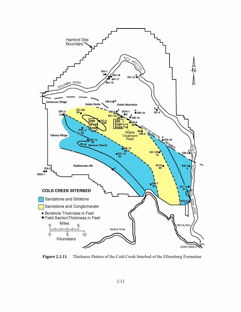
At the WTP site, the Ellensburg Formation consists of four members (Figure 2.1.3). These are, from oldest to youngest, the Mabton (Figure 2.1.10), the Cold Creek (Figure 2.1.11), the Selah (Figure 2.1.12), and the Rattlesnake Ridge (Figure 2.1.13) interbeds. The sediments dominantly consist of sand, silt, clay, and minor ash and are well consolidated, with some partly cemented. Except for the Cold Creek Interbed, these sediments indicate low-energy deposits with the main channels of the rivers away from the WTP site. Also associated with the river deposits are volcanic ash layers derived from eruptions in the Pacific Northwest. Some of these eruptions occurred as far away as southern Oregon and Idaho. During the hiatuses between times of sediment and ash deposition, soils developed. Some soil layers are as much as several feet thick.

2.11
Figure 2.1.10. Thickness Pattern of the Mabton Interbed of the Ellensburg Formation
2.12
Figure 2.1.11. Thickness Pattern of the Cold Creek Interbed of the Ellensburg Formation

2.13
Figure 2.1.12. Thickness Pattern of the Selah Interbed of the Ellensburg Formation

2.14
Figure 2.1.13. Thickness Pattern of the Rattlesnake Ridge Interbed of the Ellensburg Formation

2.15
2.1.3 Ringold Formation
The Ringold Formation (Figure 2.1.2) overlies the Columbia River Basalt Group. At the WTP, it consists of fluvial sediments deposited by the ancestral Columbia River system between about 5 and 10 Ma and forms the Unit A gravels member of Wooded Island (Figure 2.1.2). The gravels are matrix-supported, pebble to cobble gravels with a fine to coarse sand matrix. Interbedded lenses of silt and sand are common. Cemented zones within the gravels are discontinuous and of variable thickness.
2.1.4 Hanford Formation
The Hanford formation (Figure 2.1.2) overlies the Ringold Formation. The Hanford formation consists of glaciofluvial sediments deposited by cataclysmic floods from Glacial Lake Missoula between about 2 Ma and 13 Ka. These deposits are subdivided under the WTP into 1) lower gravel-dominated and 2) upper sand-dominated.
2.1.4.1 Lower Gravel-Dominated Sediment
The lower sediment generally consists of coarse-grained basaltic sand and granule to boulder gravel. Many exposures on the Hanford Site (e.g., various burrow pits) show that these deposits typically have an open framework texture, massive bedding, plane to low-angle bedding, and large-scale planar cross bedding in outcrop. The gravel-dominated sediment was deposited by high-energy floodwaters in or immediately adjacent to the main cataclysmic flood channelways.
2.1.4.2 Upper Sand-Dominated Sediment
The upper sediment consists of fine- to coarse-grained sand and granule gravel with sparse layers of Cascade ash deposits. The sands typically have high basalt content and are commonly referred to as black, gray, or salt-and-pepper sands. They may contain small pebbles and rip-up clasts, pebble-gravel interbeds, and silty interbeds less than 3 ft (1 m) thick. The silt content of the sands is variable, but where the silt is low, a well-sorted texture is common. The sand facies was deposited adjacent to main flood channelways during the waning stages of flooding.
2.1.4.3 Holocene Sediments
Holocene sediments at Hanford typically consist of active and stabilized sand dunes as well as localized alluvial fans and stream deposits. These sediments form a thin veneer across the WTP site.
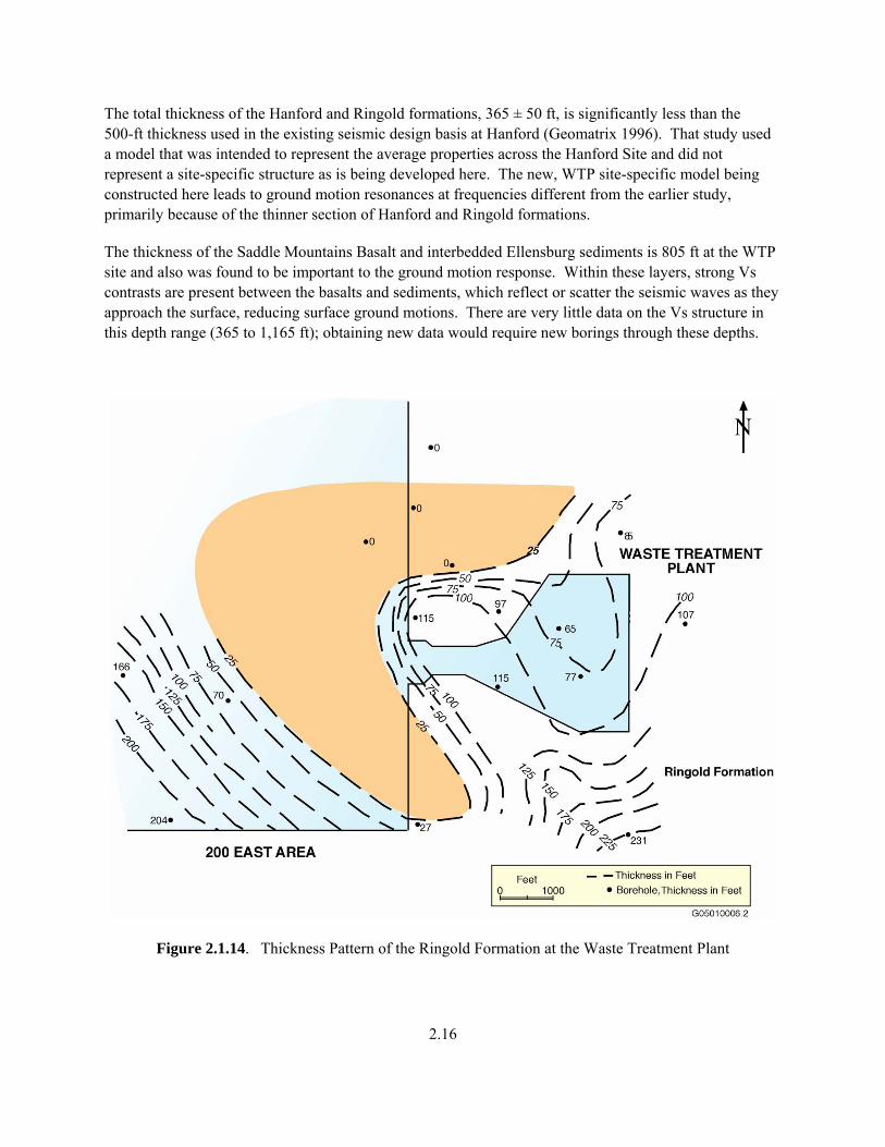
2.1.5 Thickness of Units at Waste Treatment Plant Site
Based on numerous lithologic logs in the area of the WTP site, a table of thicknesses for the geologic units present at the WTP has been developed. Figures 2.1.14 and 2.1.15 show the thickness of the Hanford and Ringold formations; previous sections provided the thickness of the Saddle Mountains Basalt and interbedded sediments of the Ellensburg Formation. These thicknesses are used for site response models. Table 2.1.1 lists these thickness values and uncertainties chosen.
2.16
The total thickness of the Hanford and Ringold formations, 365 ± 50 ft, is significantly less than the 500-ft thickness used in the existing seismic design basis at Hanford (Geomatrix 1996). That study used a model that was intended to represent the average properties across the Hanford Site and did not represent a site-specific structure as is being developed here. The new, WTP site-specific model being constructed here leads to ground motion resonances at frequencies different from the earlier study, primarily because of the thinner section of Hanford and Ringold formations.
The thickness of the Saddle Mountains Basalt and interbedded Ellensburg sediments is 805 ft at the WTP site and also was found to be important to the ground motion response. Within these layers, strong Vs contrasts are present between the basalts and sediments, which reflect or scatter the seismic waves as they approach the surface, reducing surface ground motions. There are very little data on the Vs structure in this depth range (365 to 1,165 ft); obtaining new data would require new borings through these depths.
Figure 2.1.14. Thickness Pattern of the Ringold Formation at the Waste Treatment Plant

2.17
Figure 2.1.15. Thickness Pattern of the Hanford Formation at the Waste Treatment Plant

2.18
Table 2.1.1. Thickness of Stratigraphic Units at the Waste Treatment Plant Site
Formation Member Layer
Thickness, ft Group
Thickness, ft
Sand 165 ± 10 Hanford Gravel 100 ± 10
Ringold Ringold Unit A 100 ± 20
365 ± 50
Elephant Mountain 85 ± 15
Rattlesnake Ridge Interbed 65 ± 10
Pomona Member 185 ± 10
Selah Interbed 20 ± 10
Esquatzel Member 100 ± 10
Cold Creek Interbed 95 ± 10
Umatilla Member 150 ± 10
Saddle Mountains Basalt
Mabton Interbed 105 ± 10
805 ± 50
Priest Rapids Member
Roza Member Wanapum Basalt
Frenchman Springs Member
1100 ± 50
Grande Ronde Basalt 13000 ± 3000
14000 ±3000
2.1.6 Development of Waste Treatment Plant Site Stratigraphy with Emphasis on the Paleochannel
The sediment that overlies the Columbia River Basalt Group at the WTP site records a period of deposition and then erosion (Reidel and Horton 1999). The Ringold Formation represents evolutionary stages of the ancestral Columbia River system as it was forced to change course across the Columbia Basin by the growth of the Yakima Fold Belt. Ridges of the Yakima Fold Belt were growing during the eruption of the Columbia River Basalt Group, but their influence was negated by the nearly complete burial of the ridges by each new basalt eruption. After the last major basalt eruption, the ridges began to develop significant topography. The highest topography first developed where the ridges intersected the north-south trending Hog Ranch-Naneum Ridge anticline along the western boundary of the Pasco Basin (Figure 2.1.1). Continued uplift of the Hog Ranch-Naneum Ridge anticline and the ridges of the Yakima Fold Belt forced the Columbia River and its confluence with the pre-Snake River (Salmon-Clearwater River) eastward. By 10.5 million years ago, the Columbia River was flowing along the western boundary of the Hanford Site and then turned southwestward through Sunnyside Gap southwest of Hanford and
2.19
south past Goldendale, Washington. This was the time of the Snipes Mountain conglomerate (Figure 2.1.2) and marked the end of the Ellensburg Formation time.
Ringold Formation time began approximately 8.5 million years ago when the Columbia River abandoned Sunnyside Gap, a water gap through the Rattlesnake Hills along the southwestern margin of the Hanford Site, and began to flow across the Hanford Site, leaving the Pasco Basin through the current Yakima River water gap along the southeastern end of the Rattlesnake Mountain anticline. The northern margin of the 8.5 million-year-old Ice Harbor basalt controlled the Columbia River channel as it exited the Pasco Basin.
The first record of the Columbia River at Hanford is in the extensive gravel and interbedded sand of Unit A, Ringold Formation member of Wooded Island (Figure 2.1.2). The Columbia River was a gravelly braided plain and widespread paleosol system that meandered across the Hanford Site.
At about 6.7 million years ago, the Columbia River abandoned the Yakima River water gap along the southeastern extension of Rattlesnake Mountain and began to exit the Pasco Basin through Wallula Gap (Figure 2.1.1), the present water gap where the Columbia River leaves Washington. The main channel of the Columbia River in the Pasco Basin was still through Hanford and the 200 Areas. At this time, the Columbia River sediments changed to a sandy alluvial system with extensive lacustrine and overbank deposits. A widespread lacustrine-overbank deposit called the Lower Mud was deposited over much of the Hanford Site at this time and is a nearly continuous feature under the 200 West Area and much of the 200 East Area (Reidel and Horton 1999).
The Lower Mud was then covered by another extensive sequence of gravels and sands. The most extensive of these is called Unit E, Ringold Formation member of Wooded Island, but locally other sequences are recognized (e.g., Unit C). Unit E is one of the most extensive Ringold gravels and appears to be continuous under much of the 200 Areas.
The Columbia River sediments became more sand-dominated after 5 million years ago when more than 90 m (295 ft) of interbedded fluvial sand and overbank deposits accumulated at Hanford. These deposits are collectively called the Ringold Formation member of Taylor Flat (Figure 2.1.2). The fluvial sands of the Ringold Formation member of Taylor Flat dominate the lower cliffs of the White Bluffs.
Between 4.8 million years ago to the end of Ringold time at 3.4 million years ago, lacustrine deposits dominated Ringold deposition. A series of three successive lakes is recognized along the White Bluffs and elsewhere along the margin of the Pasco Basin. The lakes probably resulted from damming of the Columbia River farther downstream, possibly near the Columbia Gorge. The lacustrine and related deposits in the Pasco Basin are collectively called the member of Savage Island (Figure 2.1.2). Because of the extensive lake that covered most of the Pasco Basin, the velocity of the Columbia River was greatly reduced and thus did not deposit gravels over the Hanford area during this period.
At the end of Ringold time, the Pacific Northwest underwent regional uplift, resulting in a change in base level for the Columbia River system. Uplift caused a change from sediment deposition to regional incision and sediment removal. Regional incision is especially apparent in the Pasco Basin where nearly 100 m (328 ft) of Ringold sediment have been removed from the Hanford area and the WTP. The

2.20
regional incision marks the beginning of Cold Creek time (Figure 2.1.2) and the end of major deposition by the Columbia River.
Regional incision and erosion by the Columbia River during Cold Creek time is most apparent in the surface elevation change of the Ringold Formation across the Hanford Site. The elevation of the surface of the Ringold Formation decreases toward the present-day Columbia River channel. In the southwestern part of the Pasco Basin near the 200 West Area, less incision of the Ringold Formation occurred than at the 200 East Area. The greatest amount of incision is near the current river channel. This increasing incision into the Ringold Formation toward the current Columbia River channel occurred with time as the channel of the Columbia River moved eastward across Hanford.
As incision of the Columbia progressed eastward across Hanford, the eroded surface of the Ringold Formation in the 200 West Area was left at a higher elevation than at the 200 East Area. This also indicates that the surface of the Ringold in the 200 West Area is older than that in the 200 East Area and thus was exposed to weathering processes for a much longer time. This higher surface at the 200 West Area accounts for the isolated deposits of the fluvial sands of the Ringold Formation member of Taylor Flat. Isolated pockets of these fluvial sands remained as the Columbia River channel progressed eastward. At the 200 East Area, the ancestral Columbia River was able to cut completely through the Ringold Formation to the top of the basalt, forming what is termed the paleochannel in this report. The paleochannel can be traced from Gable Gap across the eastern part of the 200 East Area and WTP and to the southeast.
The Cold Creek unit (Figure 2.1.2) is the main sediment that records the geologic events between the incision by the Columbia River and the next major event, the Missoula floods (Hanford formation Figure 2.1.2). The older Ringold surface at the 200 West Area was exposed to weathering, resulting in the formation of a soil horizon on its surface. Because the climate was becoming arid, the resulting soil became a pedogenically altered, carbonate-rich, cemented paleosol. The development of this carbonate-rich paleosol is much greater in the 200 West Area than in the 200 East Area due to longer exposure of the surface. This ancient paleosol is referred to as the lower Cold Creek unit.
During the Cold Creek time, fluvial deposits from major rivers (Yakima, Salmon-Clearwater-Snake, and Columbia) were deposited on the Ringold Formation in the Pasco Basin. In the central Pasco Basin east of 200 East Area, a thick sheet of gravel, informally called the Cold Creek unit (Figure 2.1.2), overlies the Ringold Formation. In earlier literature at Hanford, they were called the Pre-Missoula gravels. The Cold Creek unit is up to 25 m (82 ft) thick and may be difficult to distinguish from the underlying Ringold gravels and overlying Hanford deposits. The Cold Creek unit gravels are interpreted to be a Pleistocene-age, post-Ringold incision phase of the Columbia River as it flowed through Gable Gap.
As the Columbia River incised into the Ringold Formation near the 200 East Area, eroded and reworked Ringold sediment was incorporated into this later phase of the Columbia River. In the eastern part of the 200 East Area, Ringold-type gravels have been encountered that more closely resemble Missoula flood gravels, with characteristics like caliche cementation similar to the Cold Creek unit. These sediments are interpreted as Pliocene to Pleistocene age deposits of the Columbia River, and descriptions commonly include this uncertainty.

2.21
During the Pleistocene, cataclysmic floods inundated the Pasco Basin several times when ice dams failed in northern Washington. Current interpretations suggest as many as 100 flooding events occurred as ice dams holding back glacial Lake Missoula repeatedly formed and broke. In addition to larger major flood episodes, there were probably numerous smaller individual flood events. Deciphering the history of cataclysmic flooding in the Pasco Basin is complicated, not only because of floods from multiple sources but also because the paths of Missoula floodwaters migrated and changed course with the advance and retreat of the Cordilleran Ice Sheet.
In addition to sedimentological evidence for cataclysmic flooding in the Pasco Basin, high-water marks and faint strandlines occur along the basin margins. Temporary lakes were created when floodwaters were hydraulically dammed, resulting in the formation of Lake Lewis behind Wallula Gap. Formation of this lake and its overflow may have initiated in the Columbia Gorge, as indicated by similar high-water marks both upstream and downstream of Wallula Gap. High-water mark elevations for Lake Lewis, inferred from ice-rafted erratics on ridges ranges from 370 to 385 m (1,214 to 1,261 ft) above sea level. The lack of well-developed strandlines and the absence of typical lake deposits overlying flood deposits suggest that Lake Lewis was short-lived.
The 200 West and 200 East Areas occur on a major depositional feature called the Cold Creek bar. Recent studies using the magnetic polarity of the sediments have shown that the earliest floods may have occurred as long ago as 2 million years. Four magnetic polarity reversals have been found in sediments from core holes in the 200 East Area. These polarity reversals have paleosols at the top of each reversed sequence of sediments. The oldest sediments occur in the ancestral Columbia River channels where the Cold Creek unit sediments occur.
Since the end of the Pleistocene, the main geologic process has been wind. After the last Missoula flood drained from the Pasco Basin, winds moved the loose, unconsolidated material until vegetation was able to stabilize it. Stabilized sand dunes cover much of the Pasco Basin, but there are areas, such as along the Hanford Reach National Monument, where active sand dunes remain.
2.1.7 Nature of the Paleochannel Under the Waste Treatment Plant Site
The subsurface expression of the paleochannel is defined by the surface of the uneroded remnants of the Ringold Formation and Columbia River Basalt Group. The Columbia River Basalt Group gently tilts south (Figure 2.1.16) toward the axis of the Cold Creek syncline and appears to have no significant erosion under the WTP. The channel now is filled with sediments of the Hanford formation. No Columbia River Basalt Group lavas have been eroded from the channel under the WTP (Figure 2.1.17).
Two deeper parts of the main channel are in the vicinity of the WTP (Figures 2.1.17 and 2.1.18). The deeper one is west of the WTP; the shallower one is under the WTP. The elevation of the surface of the paleochannel on the west side of WTP site is approximately 414 ft above mean sea level (MSL). The elevation of the surface of the paleochannel on the east side of the WTP site is approximately 438 ft above MSL. The maximum relief on the surface of the paleochannel under the WTP site is approximately 70 ft. The deepest elevation (lowest point) under the WTP is 370 ft above MSL.

2.22
The topography of the surface defined by the contact between the Hanford and Ringold formations was examined for its effect on the ground motion response, by varying both the Ringold Formation thickness and velocity, and was found not to have a major effect. The existing site-wide model had the top of the Ringold Formation at a depth of 250 ft and alternative Vs models for the Ringold (Geomatrix 1996), which are similar to those found in this study.
Figure 2.1.16. Elevation Contours on the Surface of the Columbia River Basalt Group. The grey line shows the location of the cross section in Figure 2.1.17.

2.23
Figure 2.1.17. Geologic Cross Section Showing the Paleochannel in the 200 East Area. Vertical scale is equal to horizontal scale.
Figure 2.1.18. Elevation Contours Showing Relief on the Surface of the Ringold Formation in the 200 East Area. The contours show the topography on the surface of the paleochannel.
2.24
2.2 Density of Units at Waste Treatment Plant Site
Densities of the sediments, basalts, and interbeds were measured in the late 1970s and early 1980s by the U.S. Geological Survey (USGS) (Robbins et al. 1979, 1983) using a borehole gravity meter. Table 2.2.1 summarizes these measurements and displays the average values from the available boreholes.
These densities are used to develop the site response modeling. The somewhat lower density for the Wanapum Basalt (2.7 versus 2.8 for some flows) reflects an average over the entire depth extent, including interflow zones in these basalts.
The shallow Hanford formation was subdivided into an upper sand-dominated layer and a lower gravel-dominated layer. Shannon & Wilson, Inc. (2000) determined the following values (converted for comparison to USGS values above):
Unit Density, pcf Density, gm/cc Hanford sands 110 1.76 Hanford gravels 120 1.92 Ringold Formation 125 2.00
The ground motion response model uses the Shannon & Wilson (2000) model for the Hanford sands and gravels but retains the higher density for the Ringold Formation at the WTP site.
Lower Ringold densities are observed to vary from 2.0 to 2.3 gm/cc, systematically with lithology. The value of 2.3 was chosen to be used to represent the gravel characteristic that is thought to underlie the WTP site. If a sand- or silt-dominated Ringold were assumed, a lower value would be appropriate. Note that the interbed densities are in the range 2.1 to 2.3 gm/cc, even at depths near 1,000 ft. The final model, Table 2.2.2, adopts the Shannon & Wilson (2000) Hanford sand and gravel values.

2.25
Table 2.2.1. Densities of Units from Borehole Gravity Measurements (gm/cc). The Upper Ringold corresponds to the Taylor Flat member, and the remaining Ringold units correspond to the Wooded Island member in Figure 2.1.2.

2.26
Table 2.2.2. Formation-Based Densities for the WTP Site Response Model
Formation Member
Layer Thickness,
ft Group Thickness,
ft
Density,gm/cc
Sand 165 ± 10
1.76 Hanford
Gravel 100 ± 10
1.92
Ringold Ringold Unit A 100 ± 20
365 ± 50
2.3
Elephant Mountain 85 ± 15
2.8
Rattlesnake Ridge Interbed 65 ± 10
2.1
Pomona Member 185 ± 10
2.8
Selah Interbed 20 ± 10
2.3
Esquatzel Member 100 ± 10
2.7
Cold Creek Interbed 95 ± 10
2.3
Umatilla Member 150 ± 10
2.7
Saddle Mountains Basalt
Mabton Interbed 105 ± 10
805 ± 50
2.1
Priest Rapids Member
Roza Member Wanapum Basalt
Frenchman Springs Member
1100 ± 50 1100 ± 50 2.7
2.3 Velocity Model for Hanford and Ringold Sediments
This section describes the data and the analysis used to construct a model for the shear wave velocity structure of the sedimentary Hanford and Ringold layers at the WTP site. Data on the Vs structure of the Hanford and Ringold formations described below were collected recently (1999 and 2004) using state-of-the-art methods.
In 1999, a comprehensive geotechnical field and laboratory investigation of the WTP site was performed by Shannon & Wilson (see Shannon & Wilson 2000). Because it was known from other Hanford Site projects that the site is very competent for bearing purposes, the emphasis was placed on geophysical measurement to develop dynamic soil properties for soil-structure interaction analysis.

2.27
Among borings, test pits, and laboratory testing, the investigation included
• 26 seismic cone penetrometer tests (SCPTs) (Figure 2.3.1), extending to depths of between 75 ft and 100 ft, to more clearly define stratigraphy and to obtain additional shear wave and compressional wave velocities of the subsurface soils
• 4 deep borings in each of the major process building areas to a depth of 260 ft to 270 ft
(Figure 2.3.2) – Downhole seismic testing was performed in each of the 4 deep borings to obtain shear and compressional wave velocities of the subsurface soils.
• 4 refraction survey lines to provide measurements of shear and compressional shear wave
velocities to depths of approximately 350 ft – The refraction lines cross all major buildings in the facility.
Data from the 26 SCPTs and the 4 downhole borings are described in Sections 2.3.1 and 2.3.2, respectively.
The refraction survey lines were considered to be inferior to the SCPT and downhole data, and the deeper data were ambiguous regarding the depth and material (Ringold Unit A versus basalt) sampled by the refraction surveys. Refraction profiling is more sensitive to assumptions about the actual path the seismic waves travel compared to the SCPT and downhole methods. There are sufficient data from these two methods, so the refraction data were not considered further.
Additional data were collected in 2004 to resolve questions about the earthquake ground motion response of the WTP. A borehole was drilled down to the top of the basalt, 540 ft deep and approximately 6,000 ft west-southwest of the WTP site, and lined with PVC casing. This position was chosen because of its geologic similarity to that inferred under the WTP (the Ringold had not been so eroded) and its location outside an existing contaminated groundwater aquifer, making it readily accessible. Data also were collected using existing boreholes (with stainless steel casing) surrounding the WTP site that could be logged to shallower depth (up to 260 ft, essentially through the Hanford formation), avoiding the contaminated aquifer.
The velocity measurements that were made included
• downhole Vs and Vp measurements in the 540-ft-deep borehole (named the Shear Wave Borehole, SWVB; Figure 2.3.2) – Measurements made include measurements to detect anisotropy (Section 2.3.3).
• downhole Vs measurements in four additional boreholes (Figure 2.3.2) to depths of 200 to 260 ft
(Section 2.3.3) • in-hole suspension logging of the 540-ft-deep SWVB to confirm the results of the downhole
method (Section 2.3.4) – This method required a water-filled borehole, and well construction failures limited the measurement depth range in this borehole to below 361 ft. A paired second
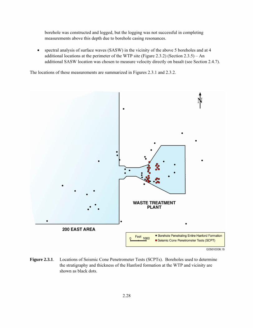
2.28
borehole was constructed and logged, but the logging was not successful in completing measurements above this depth due to borehole casing resonances.
• spectral analysis of surface waves (SASW) in the vicinity of the above 5 boreholes and at 4
additional locations at the perimeter of the WTP site (Figure 2.3.2) (Section 2.3.5) – An additional SASW location was chosen to measure velocity directly on basalt (see Section 2.4.7).
The locations of these measurements are summarized in Figures 2.3.1 and 2.3.2.
Figure 2.3.1. Locations of Seismic Cone Penetrometer Tests (SCPTs). Boreholes used to determine the stratigraphy and thickness of the Hanford formation at the WTP and vicinity are shown as black dots.

2.29
Figure 2.3.2. Locations of Downhole and Suspension Log Velocity Measurements and SASW Measurements. The Shannon & Wilson measurements are the four triangles (BD-8, BD-23, BD-35, and BD-47) within the WTP footprint. The Shear Wave Borehole (SWVB), where both downhole and suspension data were taken, is shown as a square. Additional downhole velocity measurement boreholes are shown as squares with well numbers. The SASW profile sites, lengths, and map orientations are shown as lines, with the C indicating the location of the central receiver.
2.3.1 Shannon & Wilson Seismic Cone Penetrometer Velocities at the Waste Treatment Plant Site
The 1999 seismic cone penetrometer data were collected by Advanced Research Associates (Shannon & Wilson 2000, Section 4.5 and Appendix C). Both Vp and Vs measurements were made every 3 ft at 26 locations (Figure 2.3.1) at the WTP site, to depths ranging from 75 to 100 ft. The locations represent the footprint of four major structures constituting the WTP complex. The offset distance from the top of the penetrometer rod was 6 ft for the compressional wave source and 3 ft for the shear wave source. Therefore, velocities measured at depths comparable to these offset distances may not be as accurate due to raypath effects.

2.30
These data were reviewed and are considered to be the best source of accurate shallow velocity data, and are all overlaid in Figure 2.3.1.1. These data were statistically averaged and then blended with the other shallow velocity data from downhole and SASW measurements described in Sections 2.3.2 through 2.3.5.
ARA SCPT
0
50
100
150
0 500 1000 1500 2000 2500
Vs (ft/sec)
Dep
th (f
t)
SCPT-13SCPT-11SCPT-12SCPT-14SCPT-09SCPT-08SCPT-10SCPT-06SCPT-01SCPT-05SCPT-04SCPT-03SCPT-20SCPT-18SCPT-16SCPT-17SCPT-19SCPT-21SCPT-22SCPT-24SCPT-26SCPT-28SCPT-27SCPT-25SCPT-23SCPT-02
Figure 2.3.1.1. Summary of Seismic Cone Penetrometer Vs Profiles
2.3.2 Shannon & Wilson Downhole Velocities from the Waste Treatment Plant Site Investigation
The 1999 Blackhawk Geometrics downhole measurements (Shannon & Wilson 2000, Section 2.3.2 and Appendix B) were made to depths of 260 to 270 ft. The locations of these boreholes (Figure 2.3.2) are also (as with most of the SCPT locations) directly under four of the major structures constituting the WTP complex. The travel time and measurement geometry are included as tables in Blackhawk’s Appendix B. The data were taken with a source that was offset from the top of the borehole by 20 ft, so near-surface velocities may not be very accurate due to raypath complications. Consistent results are obtained from these four boreholes and, in the uppermost 100 ft, also are consistent with the results of the SCPT measurements.
The travel times, corrected by the slant distance (due to the 20-ft offset source), were plotted on reduced velocity diagrams by removing an average slope of 2,000 fps from the travel times (Figures 2.3.2.1 through 2.3.2.4). Doing so enhances changes in slope to estimate depth ranges having near-constant velocity. After interpretation by fitting by eye, data points were selected that represented straight-line segments and were fitted using least squares. The intersections of different velocity segments were calculated from the least-square fits.

2.31
Similar results were found at the four boreholes, although there were problems interpreting several parts of the data. In borehole BD-8, there was an apparent high-velocity interval in the 170- to 220-ft depth range. This was considered inconsistent with the other data, and a straight-line was fit from depths of 170 to 260 ft. In borehole BD-23, there were inconsistent data at 35- and 40-ft depths that were excluded from the fit. In borehole BD-35, it appears that there was a shift of the travel times at depths greater than 50 ft, as might occur if a different cycle of the signal became more visible.
The results of this reinterpretation are shown in Table 2.3.2.1 and superimposed on a plot of velocity versus depth in Figure 2.3.2.5. Four layers are interpreted, each with similar velocity and depth extent.
Table 2.3.2.1. Shannon & Wilson Block Velocity Model from Downhole Data
Layer 1 2 3 4 Hole No.
z Vs se
z Vs se
z Vs se
z Vs se
Notes BD-08
0 627 (9)
15 1225 (56)
63 1756 (34)
169 2510 (133)
1
BD-23
0 532 (20)
16 1308 (212)
58 1678 (37)
159 2280 (37)
2
BD-35
0 531 (20)
16 1114 (31)
55 1991 (27)
196 2387 (79)
3
BD-47
0 433 (53)
14 1156 (61)
52 1863 (22)
186 2332 (70)
Notes: z, depth to layer top; Vs, shear wave velocity; se, standard error of velocity 1: Layer 4 high velocity; 2: Layer 2 did not fit 2 points;
3: Layer 3 has travel time offset, affects layer depths
A comparison of Figure 2.3.2.5 to the original interpretation Figure 2.3.2.6 (Shannon & Wilson 2000, Figure 7-25), shows less scatter for the reinterpreted velocities compared to the original interpretation as interval velocities. The high interval velocities at shallow depth (25-50 ft: BD-23; 50-75 ft: BD-35) noted above are apparent, as are most of the high interval velocities at depths below 175 ft from borehole BD-08.
Figure 2.3.2.7 compares the downhole data from the four boreholes to the 26 SCPT profiles from the previous section. They are in general agreement with the SCPT data at depths less than 100 ft, but the velocities from the downhole block model are somewhat lower around the 50-ft depth and near the surface. Faster velocities (shorter travel times) from the shallowest downhole measurements would result if raypaths are refracted by a velocity gradient near the surface, but are still interpreted based on the assumed geometric straight-line distance. Therefore, this does not explain the lower downhole velocities at very shallow depths (15 ft and less). Ten feet of this shallow material were excavated, filled, and compacted, so the very shallow velocities ultimately are not used in the ground motion response modeling.

2.32
The comparison of the downhole and SCPT Vs profiles presented in Figure 2.3.2.7 shows the range of velocity profiles available for the upper 100 ft (downhole and SCPT) and the range of models for depths between 100 and 270 ft (four downhole only). This set of data, taken from a tight geographical area representing the actual footprints of four major structures constituting the WTP complex, will be further compared and averaged with the additional downhole measurements (Section 2.3.3) and SASW measurements (Section 2.3.4). The latter were taken over a broader geographical area. All data are later combined into final models for the Hanford and Ringold formation Vs profile in Section 2.5.
Figure 2.3.2.1. Reinterpretation of Shannon & Wilson Downhole Data from BD-08
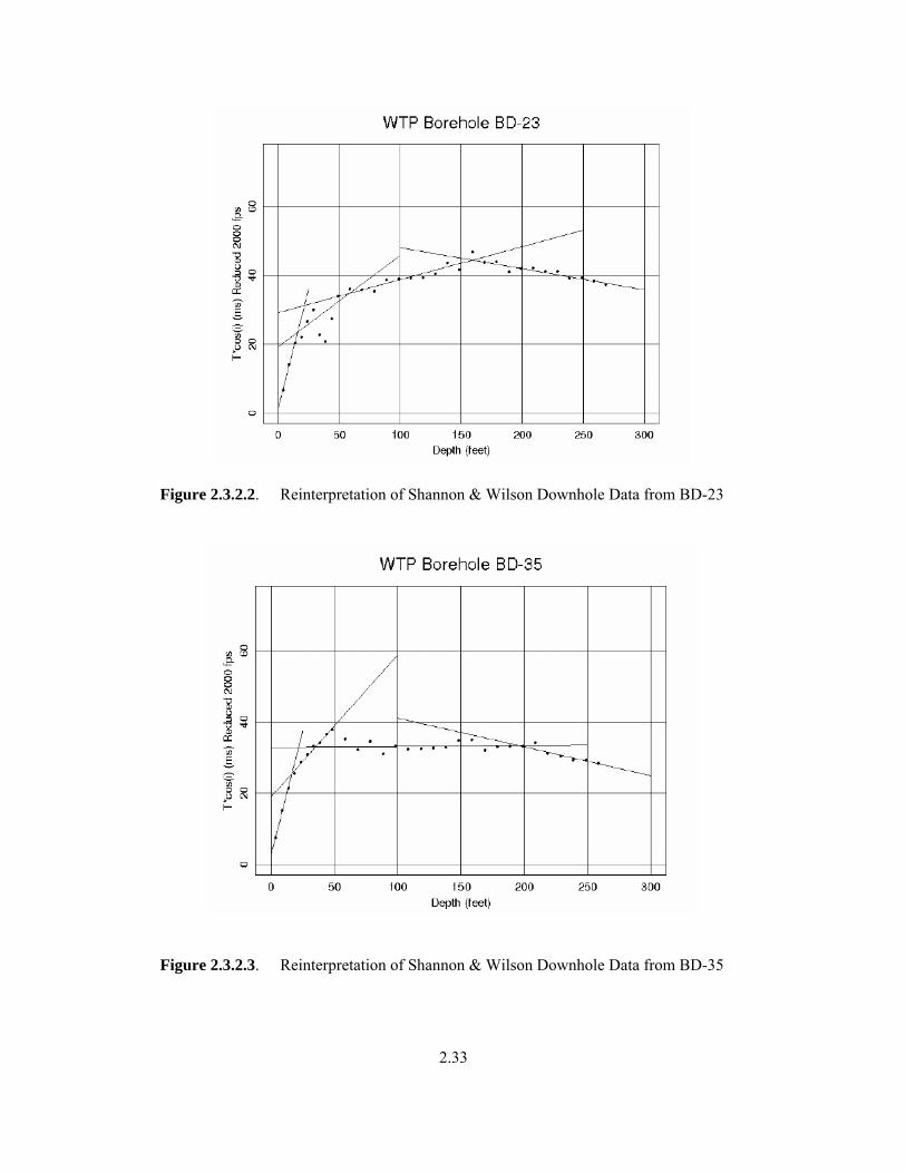
2.33
Figure 2.3.2.2. Reinterpretation of Shannon & Wilson Downhole Data from BD-23
Figure 2.3.2.3. Reinterpretation of Shannon & Wilson Downhole Data from BD-35

2.34
Figure 2.3.2.4. Reinterpretation of Shannon & Wilson Downhole Data from BD-47

2.35
0
50
100
150
200
250
300
0 1000 2000 3000 4000 5000
Vs, fps
Dept
h, ft
Figure 2.3.2.5. Reinterpreted Shannon & Wilson Downhole Shear Wave Velocity Profiles

2.36
0
50
100
150
200
250
300
0 500 1000 1500 2000 2500 3000 3500 4000
Vs, ft/sec
Dep
th to
Sur
face
, ft
BD-8A
BD-23
BD-35
BD-47
River Protection Project Waste Treatment Plant
Subcontract No. WSTC99-1036
S-WAVE VELOCITY VS. DEPTHDOWNHOLE SEISMIC STUDIES
May 2000 H-1616-51
FIG. 7-25 SHANNON & WILSON, INC.Geotechnical and Environmental Consultants
Figure 2.3.2.6. Original Interpretation of Downhole Data as Interval Velocities

2.37
0
50
100
150
200
250
300
0 1000 2000 3000 4000 5000Vs, fps
Dep
th, f
t
DownholeSCPT
Figure 2.3.2.7. Comparison of Downhole to SCPT Vs Profiles at the WTP Site. These measurements were taken near the actual footprint of four major WTP structures.
2.3.3 New Downhole Velocity Measurements
A team from Northland Geophysical and Redpath Geophysics collected downhole seismic velocity surveys in six boreholes surrounding the WTP site in 2004 (Northland Geophysical 2004). The locations of these measurements are shown in Figure 2.3.2. One of the boreholes (SWVB) was specially constructed to 540 ft deep, through the entire section of the Hanford and Ringold sediments to the top of the basalt, and completed using PVC casing.

2.38
A summary of the boreholes and measurements is shown in Table 2.3.3.1. Source offset was 12 ft (14 ft for the one compressional source). Interpreted velocities at comparable depth are subject to greater inaccuracy because of the potential for raypaths not to be straight geometrical paths as is assumed in the analysis. Travel times were measured every 3 ft in the top 100 ft, every 5 ft down to 300 ft depth, and every 10 ft below that.
Table 2.3.3.1. Summary of Downhole Velocity Measurements
Borehole Number
Survey Depth, ft
Remarks
299-E24-21 230 Stainless casing, oriented transducer Shear wave only
299-E26-10 180 Stainless casing, oriented transducer Shear wave only
699-41-42 260 Stainless casing, oriented transducer Shear wave only
699-37-43 250 Carbon steel casing, unoriented transducer Shear wave only
SWVB (C4562)
530
PVC-cased Shear-wave anisotropy investigated Compression-wave measured
299-E17-21 200 Stainless casing, oriented transducer Shear wave only (20 ft from SWVB)
An example of the interpreted Vs results, from the SWVB, is shown in Figure 2.3.3.1. The velocity change from near 2,000 to 2,700 fps at the 260-ft depth reflects the change from sand-dominated to gravel-dominated Hanford formation at 250 ft. There is no apparent change in velocity at a depth of 320 ft, the contact between the lower Hanford gravels and the upper Ringold gravels (Unit E). A low-velocity zone from 390 to 424 ft is detected and correlates with a fine-grained mud layer (Lower Mud; see Section 2.1.6). The velocity below this layer, 4,310 fps, corresponds again to a gravel layer (Unit A) in the lower Ringold.
Table 2.3.3.2 and Figure 2.3.3.2 summarize the results from the six boreholes. Velocity measurements made in the SWVB and in borehole 299-E17-21, located 20 ft from SWVB, are within 5% to 8% of each other. This suggests that there may be similar velocity variability over short distances at other locations such as in the WTP area. The shear wave onset signals do not appear to be significantly worse in the steel-cased borehole 299-E17-21 compared to the SWVB.
The SWVB borehole is one of only two borehole velocity measurement of the Ringold sediments below the 250-ft depth. The only other borehole where the Ringold was present in the measurement depth range is borehole 699-41-42, which detected a velocity of approximately 4,000 fps over a 10-ft section at the bottom of the borehole. Ringold Unit A, the 4,000-fps gravel layer at the bottom of the SWVB, is

2.39
Table 2.3.3.2. Shear Wave Velocities from Downhole Measurements
Borehole Location, NAD27 Depth Range, ft Velocity, ft/sec
0 – 11 830 11 – 54 1440
54 – 135 1705 135 – 210 1860 210 – 260 2045 260 – 390 2730 390 – 424 1940
SWVB (C4562) 30°- Source
N46° 32.584’ W119° 31.947’
424 – 530 4310 0 – 10 875
10 – 50 1430 50 – 70 ?
70 – 140 1645
299-E17-21 (20’ from SWVB)
N46° 32.583’ W119° 31.955’
140 – 200 2005 0 – 6 900 6 – 36 1160
36 – 93 1400 93 – 186 1665
299-E24-21 N46° 33.016’ W119° 31.535’
186 – 230 1890 0 – 14 985
14 – 66 1570 299-E26-10 N46° 33.725’ W119° 30.778’ 66 – 180 2200
0 – 13 665 13 – 48 1435
48 – 180 1830 180 – 250 2340
699-41-42 N46° 33.195’ W119° 29.589’
250 – 260 4000 ± 0 – 14 520
14 – 90 1145 90 – 190 1810
699-37-43 N46° 32.506’ W119° 29.830’
190 – 250 2565
interpreted here from lithologic logs. Generally, in the Hanford formation, velocities 2,200 fps and below are associated with the Hanford sands, and velocities above 2,200 fps are associated with the lower Hanford gravel (and Ringold gravels).
Anisotropy was not an expected characteristic of sands and gravels, but measurements were made with four different polarizations of the shear waves, with one of the polarizations (138°) oriented parallel with the predominant southeastern flow directions that laid down the sediments. Travel times corresponding to

2.40
the different polarizations agreed to within 1%, indicating no anisotropy. The velocities in the southeast and perpendicular directions are listed in Table 2.3.3.3
Compressional wave measurements were made at the SWVB borehole only, because the metal casing in the other boreholes obscures the compression wave onset. Table 2.3.3.3 shows the resulting Vp values and calculated Poisson’s ratio for the different depth intervals. Poisson’s ratio (or the ratio Vp/Vs) in sedimentary materials becomes an important element in the development of the velocity model. Much of the data available for deeper sedimentary layers (the interbeds in the Saddle Mountains Basalt) is only Vp, and Poisson’s ratio must be assumed in the modeling of the SASW data (see Section 2.3.5).
Table 2.3.3.3. SWVB Vs Anisotropy, Vp, and Poisson’s Ratios. The two polarization orientations, 138° and 48°, are approximately parallel to and perpendicular to the depositional flow direction, respectively.
Velocity, ft/sec
Shear Wave Depth Range, ft
48° 138°
Compression Wave
Poisson’s Ratio
(48° Source)
0 – 11 830 770 1200 0.04 11 – 54 1440 1430 2190 0.12
54 – 135 1705 1710 2525 0.08 135 – 210 1860 1895 3180 0.24 210 – 260 2045 2125 3180 0.15 260 – 390 2730 2755 5475 0.33 390 – 424 1940 2015 5475 0.43 424 – 530 4310 4335 9440 0.37
Figure 2.3.3.3 shows a comparison of the Northland/Redpath downhole Vs profiles to those produced from the WTP site investigation downhole and SCPT (Shannon & Wilson 2000). Lower velocities are found in the upper 90 ft at two boreholes south of the WTP site (SWVB and 37-43) compared to those from the WTP site itself. The other three Northland/Redpath profiles are in better agreement. There is general agreement between the WTP downhole and Northland/Redpath downhole velocity profiles below 90-ft depths to a depth of 250 ft.

2.41
Figure 2.3.3.1. Interpreted Shear Wave Velocity Profile at the Shear Wave Borehole (SWVB)

2.42
0
100
200
300
400
500
600
0 1000 2000 3000 4000 5000Vs, fps
Dep
th, f
tRedpath
Figure 2.3.3.2. Shear Wave Velocity Profiles from Downhole Measurements
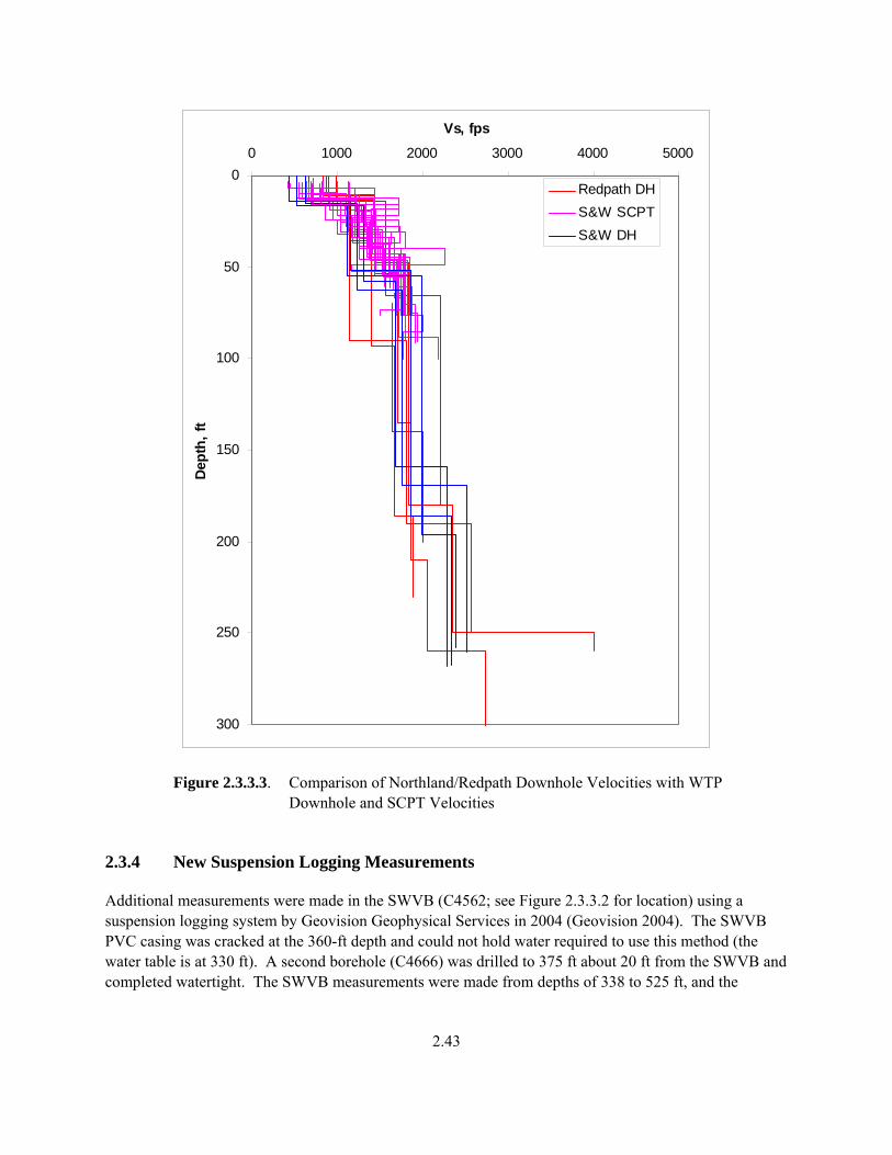
2.43
0
50
100
150
200
250
300
0 1000 2000 3000 4000 5000
Vs, fps
Dep
th, f
tRedpath DHS&W SCPTS&W DH
Figure 2.3.3.3. Comparison of Northland/Redpath Downhole Velocities with WTP Downhole and SCPT Velocities
2.3.4 New Suspension Logging Measurements
Additional measurements were made in the SWVB (C4562; see Figure 2.3.3.2 for location) using a suspension logging system by Geovision Geophysical Services in 2004 (Geovision 2004). The SWVB PVC casing was cracked at the 360-ft depth and could not hold water required to use this method (the water table is at 330 ft). A second borehole (C4666) was drilled to 375 ft about 20 ft from the SWVB and completed watertight. The SWVB measurements were made from depths of 338 to 525 ft, and the

2.44
measurements in the replacement borehole C4666 were made from 4 to 370 ft. The measurement interval was 1.64 ft (0.5 m). However, the waveforms for the data above a depth of 360 ft prevented a useful analysis and were not reported. It was thought that the well construction, cementing of the casing, and attempts to plug the leak at the 360-ft depth may have prevented obtaining clear signals using this method.
The results of the suspension logging from 360 to 525 ft are shown in Figure 2.3.4.1.
The log begins with a 2,000 fps Vs between 360- and 430-ft depths. As noted for the downhole log in Section 2.3.3, this interval is in the Lower Mud unit of the Ringold Formation, and the fine-grained mud has a low velocity. Below the 440-ft depth, the log detects layers with relatively high Vs of 5,200 to 6,400 fps alternating with relatively low Vs of 2,000 to 2,500 fps. This is a different result from the SWVB downhole log, where an average velocity of 4,300 fps was determined, although the average velocities in this interval are comparable (see below). It is not surprising that the downhole logging did not detect the low-velocity layer near 465 ft; this layer is only 10 ft thick (the same as the downhole log spacing). The low-velocity layer between 495- and 515-ft depths could have been detected between only two or three measurements. Lithologic logs showed a silt layer in this interval, so this is an additional example of fine-grained Ringold layers having characteristic low velocity.
The accumulated travel times for the suspension log were compared to those from the downhole log (Geovision 2004) and are shown in Figure 2.3.4.2. The travel times differ by only 2%, reflecting the consistency of velocities determined by the two methods.
Although it is clear that the downhole method does not have as tight a resolution of thin layers as does this suspension log, such thin layers are not expected to affect the response of the WTP site to earthquake ground motions, because ground motions of interest have lower frequency (longer wavelength).

2.45
Figure 2.3.4.1. Vs and Vp from Suspension Logging at the Shear Wave Borehole
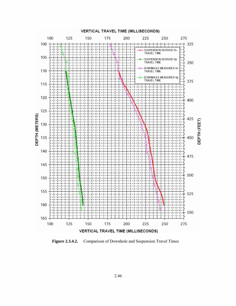
2.46
Figure 2.3.4.2. Comparison of Downhole and Suspension Travel Times

2.47
2.3.5 Spectral Analysis of Shear Waves (SASW) Measurements
Researchers from the University of Texas at Austin measured surface wave dispersion at 10 sites (Lines 1 through 9, Figure 2.3.2) in 2004 (Stokoe et al. 2005). Five of these locations were within approximately 50 ft from each of the five borehole locations that were logged using downhole methods (Sections 2.3.3 and 2.3.4; note that although six boreholes were used in the downhole logging, two were co-located). Four additional SASW measurements were made at locations along the perimeter of the WTP construction site. The tenth measurement was made approximately 6 miles northwest of the WTP location directly on basalt (location shown in Figure 2.1.7) for comparison to the other SASW sites where the basalts are 270 to 540 ft deep. The SASW method was chosen because it provided a means to extend the Vs profiles below the approximately 250-ft depth of most of the borehole measurements using a surface technique. The orientations of the profiles were chosen based on geographic logistical considerations and not for any particular geologic reasons.
Borehole logging in the water wells was performed only in the upper 200- to 250-ft depths in the Northland/Redpath study (except the SWVB to 540-ft depth; Section 2.3.3). Borehole logging to 260- to 270-ft depths was performed by Blackhawk at the WTP site (Section 2.3.2). These data therefore provide Vs information for the Hanford formation but do not provide much information for the Vs profile in the Ringold Formation. The Ringold Formation is known to be of variable thickness and is highly variable in its velocity, depending on the lithology. Muds and silts within the Ringold Formation have low Vs, near 2,000 fps, while the gravels have high Vs, near 4,000 fps, based on the section of Ringold Formation that was measured in the SWVB (Sections 2.3.3 and 2.3.4). The presence of a paleochannel that was eroded into the Ringold Formation changes its thickness from 100 ft to nearly zero at the locations where the SASW measurement were made. One of the main objectives of the SASW study was to obtain Vs profiles near the WTP site for the depth range of the Ringold Formation. These measurements could not be made in boreholes at this depth because of the contaminated groundwater plume.
Figures 2.3.5.1 through 2.3.5.5 show the SASW-derived Vs profiles superimposed on the profiles from the downhole logs at the five locations where both types of measurements were made. The SASW and the downhole logs give comparable results in the top 200 to 250 ft of the profiles (in the Hanford Formation sands and gravels). However, at sites 1, 6, and 8, (Figures 2.3.5.1, 2.3.5.3, and 2.3.5.4), higher Vs are measured using the downhole method (near 2,600 fps) in the depth range of 200 to 250 ft, while the SASW Vs remain near 2,000 fps.
At the SWVB location (Line 1, Figure 2.3.2) where the downhole log extended through the Ringold Formation to the top of basalt, the SASW profile eventually increases to near 4,000 fps at the 450-ft depth, near the same depth where the downhole log Vs increases to 4,500 fps. However, it does not seem to respond to the upper Ringold Unit E present at this location. The SASW method is not capable of detecting thin low-velocity zones at depths within the Ringold, as were seen in the suspension logging.
At site 6 (Figure 2.3.5.3), the downhole measurements barely detected a 4,000-fps layer at the bottom of the borehole. The lithologic logs for this borehole indicate the presence of Ringold Unit A, which has a Vs near 4,000 fps, comparable to that found in the SWVB location.

2.48
At site 8, the SASW Vs profile remains near 2000 fps from 150- to 400-ft depths. The downhole log detected an increase to near 2,500 fps near the 200-ft depth. This is similar to the difference between the two results found at the SWVB (site 1). In these two locations, the upper part of the Ringold Formation has not been eroded, and the SASW does not respond to the increase in Vs of the gravels of the Ringold Unit E. In contrast, the lower Ringold Unit A is picked up by the SASW measurements, with Vs near 4,000 fps, at the approximate depth from the lithologic log (which extends deeper than the downhole measurements). These are important observations in comparing the two methods, but upper Ringold structure does not affect the WTP site where most of the upper Ringold, including Unit E, has been removed by erosion.
The deeper parts of the SASW Vs profiles show increases in Vs to 4,000 to 5,000 fps. The depths to these velocity horizons are consistent with the depth to the top of the uppermost basalt flow. The SASW-determined Vs for the basalts is described later in Section 2.4.4 after the other borehole Vs data for the basalts have been presented for comparison.
Most of the remaining SASW measurements consist of those taken around the perimeter of the WTP construction site. Site 6, shown previously (Figure 2.3.5.3), comprises one of these. The SASW profiles for sites 3, 4, 5, and 7 are shown in Figures 2.3.5.6, 2.3.5.7, 2.3.5.8, and 2.3.5.9, respectively. At site 3, the Ringold Formation has been completely eroded, and the Hanford formation directly overlies the basalt at a depth of 380 ft, near where Vs jumps up to 4,000 fps.
At site 4, Vs increases to approximately 2,500 to 3,000 fps at a depth of 250 ft, and, at 400 ft, the top of basalt coincides with the jump to 4,000 fps. The Ringold Unit A gravels are found in this borehole at a depth of 260 ft. The 2,500- to 3,000-fps Vs below the 250-ft depth at this location is interpreted to be a measurement of the Ringold Vs, one that is in proximity to the WTP. This Vs value is lower than the approximately 4,000 fps Vs measured at the SWVB or at three other SASW measurement locations around the periphery of the WTP (sites 4, 5, and 6). The low Vs measured in the Ringold Formation at site 3 introduces an important uncertainty in the Vs model constructed for the Ringold Formation used in ground motion response modeling.
At site 5, Ringold Unit A gravels have a higher Vs just below 4,000 fps above 400 ft, and the basalts have a higher Vs below this depth, near 5,500 fps. At site 7, Ringold Unit A gravels have a Vs near 3,000 fps just above the 300-ft depth, but the topmost basalt flow has a low Vs, below 4,000 fps, until depths of 400 ft and greater, where it jumps to 5,000 fps.
In summary, the SASW gives results comparable to the downhole Vs surveys in the upper 250 ft where the Hanford sands and gravels represent the lithology. The Vs in the Hanford formation gradually increase from below 1,000 fps at the surface to near 2,000 fps at the bottom of the Hanford formation. The SASW variably detects the Ringold units below these depths. The Ringold Formation, where present, is variably represented by a Vs increase (relative to the Hanford formation) to a range between 2,500 and 4,000 fps. The low Vs measured at site 3 produces an important uncertainty in the Vs model constructed for the Ringold Formation that is included in ground motion response modeling.

2.49
SASW-measured Vs in the basalt is also variable and is discussed further in Section 2.4.4, where the SASW data are compared to deep borehole velocity measurements. SASW-measured Vs in basalts exposed at the surface at SASW site 10 also are compared.
Figure 2.3.5.1. Comparison of SASW Profile H1 and Downhole Logs at Site 1 (SWVB)

2.50
Figure 2.3.5.2. Comparison of SASW Profile H2 and Downhole Log at Site 2

2.51
Figure 2.3.5.3. Comparison of SASW Profile H6 and Downhole Log at Site 6

2.52
Figure 2.3.5.4. Comparison of SASW Profile H8 and Downhole Log at Site 8

2.53
Figure 2.3.5.5. Comparison of SASW Profile H9 and Downhole Log at Site 9
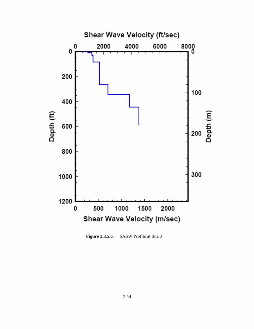
2.54
Figure 2.3.5.6. SASW Profile at Site 3

2.55
Figure 2.3.5.7. SASW Profile at Site 4
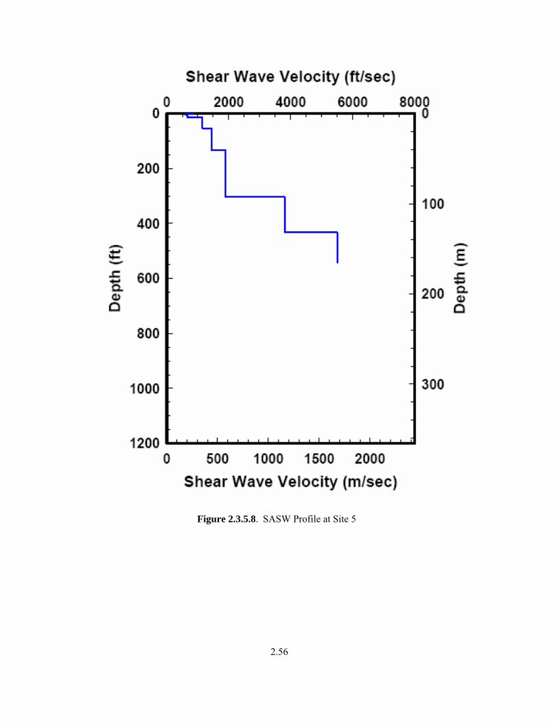
2.56
Figure 2.3.5.8. SASW Profile at Site 5

2.57
Figure 2.3.5.9. SASW Profile at Site 7
2.4 Velocity Model for Basalts and Interbeds
Over the years, numerous borehole studies have been conducted at the Hanford Site to determine the structure of the underlying Columbia River Basalt Group. These studies were conducted as parts of a variety of nuclear waste contamination and isolation studies at the Hanford Site. Many of these borehole investigations were the result of a nuclear waste repository siting study, the Basalt Waste Isolation

2.58
Project, conducted in the late 1970s through 1988. These data are the only information available on the properties of the basalts at the WTP site and are assembled and used here to constrain the elements of the velocity model below the sedimentary layers.
The locations of deep boreholes that have compressional wave borehole logs are shown in Figure 2.4.1. These logs, in the form of in-well suspension logs, or surface-to-borehole checkshot surveys, are used in Section 2.4.1 to develop the Vp model for the basalts and interbeds. Section 2.4.2 describes limited data from an historic cross-well Vp and Vs measurement and a recent suspension Vp and Vs log from a borehole drilled in the basalts 60 miles southwest of the WTP site.
There are no direct measurements of Vs or Vp/Vs in the interbeds of the Saddle Mountains Basalt and very few on-site Vp logs that measured velocities in this section. Fortunately, the one borehole that had a sonic log through the Saddle Mountains Basalt is the one closest to the WTP site, approximately 2 miles to the northwest. Measurements of Vp/Vs made in the SWVB Ringold Formation are compared to lithology in Section 2.4.3, and using the lithology of the interbeds as observed in core from the boreholes, a range of Vp/Vs values is estimated.
SASW data penetrated to a sufficient depth that they were able to measure velocities in the upper basalts and interbeds. Their locations are shown in Figure 2.3.2. One of the measurement locations was 6 miles northwest of the WTP site (see Figure 2.1.7) and was on basalt outcrop. These data appear to measure the average velocity of the basalts plus interbeds sequence but do not resolve the velocity difference between them.
Figure 2.4.1. Locations of Deep Boreholes in the Columbia River Basalt Group Referred to in this Report

2.59
2.4.1 Historical Vp Data for Basalts and Interbeds
2.4.1.1 Birdwell Sonic Logs
Applicable Birdwell sonic logs (Birdwell Division 1979) were available for boreholes DC-1, DC-19, DC-20, and RRL-2 (Figure 2.4.1). Sonic log DC-1 was recorded in both the Saddle Mountains and Wanapum basalts. Sonic logs DC-19, DC-20, and RRL-2 were recorded in the Wanapum Basalt only. For each of the sonic logs, only computer printout tables (hard copy) of the suspension logging results were available. The report for the Birdwell sonic logs was unavailable, as was the description of the tool and interpretive techniques. The seismic source is a high-frequency (kilohertz) signal recorded along the length of the sonde at one or several locations. The depth spacing between the source and receivers can be 6 ft or more. The travel time recorded over the depth interval gives a P-wave interval time or equivalently an interval velocity. Data are recorded at 1-ft intervals as the sonde is lowered in the borehole. Because the P-wave is the first arrival, automatic picking procedures are generally successful and consistent with other measurement techniques. Although an S-wave model was available in the output, these models were considered unreliable because 1) it is inherently more difficult to interpret and time the S-wave arrival and there were no supporting data traces to judge the quality of the signal or the reliability of the arrival “pick”; 2) no corroborating data were available to judge the quality of the resulting S-wave model; and 3) a description of the methodology used to derive the S-wave values was not available.
A multi-step procedure was used to generate digital data from the printed logging results. The tables of computer output were scanned, page by page, producing a bitmap image. Character recognition software then was used to develop ASCII text files of the suspension logging results. These files were plotted to correct any obvious character recognition errors. Figure 2.4.1.1 shows the P-wave velocity profile of the sonic log in borehole DC-1.
To compare the results of the Vp sonic log to other longer-wavelength (1- to 50-Hz) interpretations (i.e., SASW, checkshot), each borehole sonic log was reinterpreted. Vertical travel time was computed at 1-ft intervals from the P-wave model. Vertical travel time was then accumulated as a function of depth, resulting in a downhole travel time curve (Figure 2.4.1.2a). Linear segments were selected from this downhole travel time curve (Figure 2.4.1.2b) to construct a P-wave model that would be comparable to an engineering downhole survey (Figure 2.4.1.3). These interpreted Vp sonic log models, like any downhole interpretation, are subject to judgment but appear to be consistent with the sonic log. For example, at depths where the sonic log velocity profile is very irregular, the interpreted model tends to produce average velocities, as one would expect to occur when sampling finely stratified media using longer-period waves. For depths where the sonic P-wave model shows more consistent values with depth, the interpreted model fits these ranges nicely.
Each of the interpreted Vp sonic logs describes the P-wave seismic stratigraphy that might be comparable to a traditional downhole seismic survey employing a longer-wavelength source. In addition to the interpreted models, an alternative model was developed based on the formation intervals available with each borehole. This model is also shown in Figure 2.4.1.3. Because of the nature of the basalt deposition, a given formation can contain both high- and slow-speed material, and the Vp models based on formation interval tended to average or smooth the profile. These formation-based models were

2.60
rejected in favor of the interpreted models. Figure 2.4.1.4 shows the interpreted P-wave profiles for the applicable Birdwell sonic logs
2.4.1.2 Birdwell Checkshot Surveys
The Birdwell checkshot surveys results were available for boreholes DC-2, DC-3, DC-4, DC-6, and DC-7 (Figure 2.4.1). Values of the checkshot receiver depths together with interval and cumulative wave speeds were tabulated in available documents at PNNL. Birdwell conducted the checkshot surveys through the soils, shallow basalts and interbeds, and deeper basalts to depths greater than 2,500 ft. The checkshot survey depths were selected to determine the average P-wave speed through one or more specific formations of interest. An energetic source (vibroseis) is used to generate P-waves making phase identification for these surveys very reliable. However, because the checkshot surveys are used to confirm average vertical travel times through specific formations of interest, they cannot be reinterpreted to represent the seismic stratigraphy that would be obtained in a typical downhole survey. However, it is assumed that by combining the five checkshot surveys that were conducted for different formation combinations over a large area that includes the site, the average of these velocities should be consistent with the average of the interpreted Birdwell sonic logs. These checkshot survey P-wave models are shown in Figure 2.4.1.5. The reinterpreted P-wave sonic logs and the checkshot models are compared in Figure 2.4.1.6.
An S-wave model for the shallow basalts, interbeds, and deeper basalts was derived from the sonic logs and checkshot surveys assuming a Vp-to-Vs ratio (Vp/Vs) of 1.79 (see Section 2.4.2). These models are shown in Figure 2.4.1.7.
0
200
400
600
800
1000
1200
1400
1600
1800
2000
0 5000 10000 15000 20000 25000 30000Vp (ft/sec)
Dep
th (f
t)
WELL # DC-1DC-2 (scanned)
Sediments
Figure 2.4.1.1. Comparison of Birdwell DC-1 Sonic Log and Calibrated Sonic Log (DC-2)

2.61
y = 6E-05x - 0.0346R 2 = 0.9974
0
0.02
0.04
0.06
0.08
0.1
0.12
0.14
0.16
0.18
0 500 1000 1500 2000 2500 3000 3500
Depth (ft)
Trav
el T
ime
(sec
)
cum. TTLinear (cum. TT)
Figure 2.4.1.2a. Birdwell DC-1 Cumulative P-Wave Vertical Travel Time
-0.008
-0.006
-0.004
-0.002
0
0.002
0.004
0.006
0.008
0.01
0 500 1000 1500 2000 2500 3000 3500
Depth (ft)
TT-T
rend
(sec
)
cum. TT-lin. trend
Figure 2.4.1.2b. Birdwell DC-1 Cumulative P-Wave Vertical Travel Time Trend
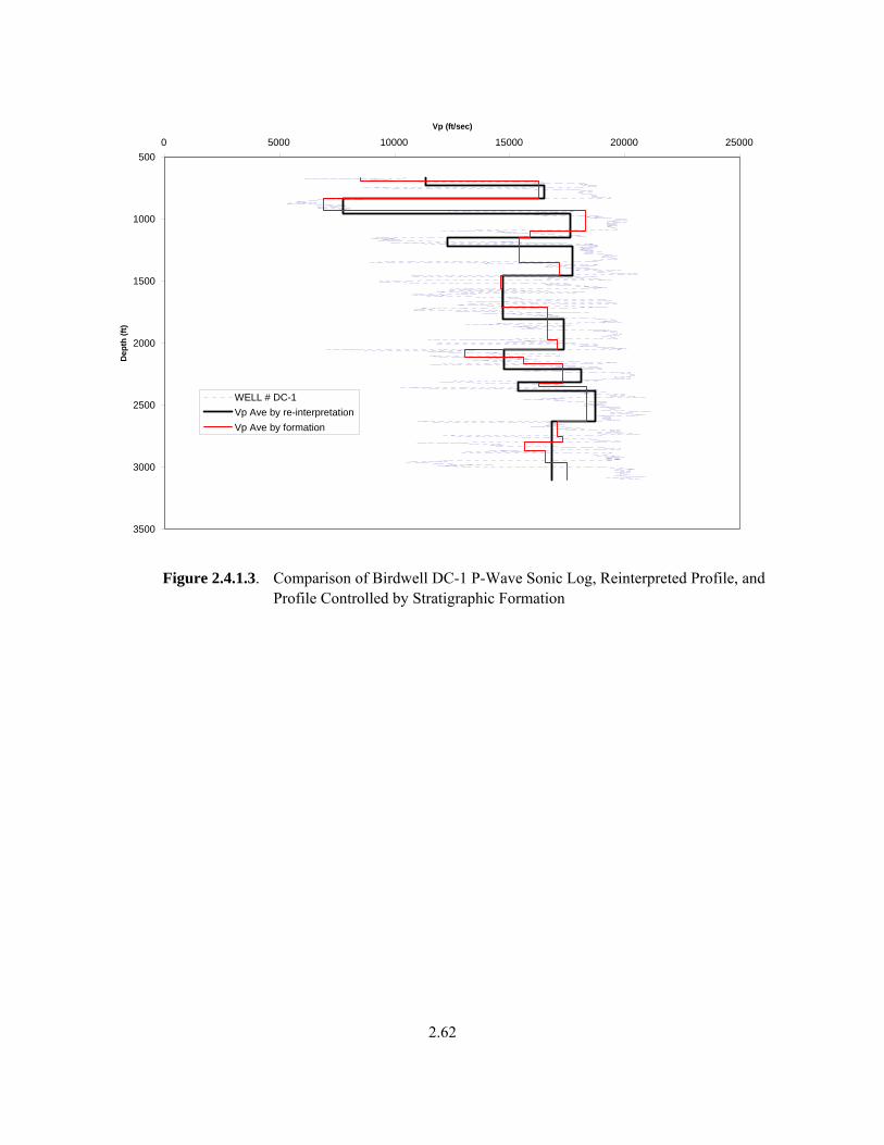
2.62
500
1000
1500
2000
2500
3000
3500
0 5000 10000 15000 20000 25000Vp (ft/sec)
Dep
th (f
t)
WELL # DC-1Vp Ave by re-interpretationVp Ave by formation
Figure 2.4.1.3. Comparison of Birdwell DC-1 P-Wave Sonic Log, Reinterpreted Profile, and Profile Controlled by Stratigraphic Formation

2.63
0.0
500.0
1000.0
1500.0
2000.0
2500.0
3000.0
3500.0
4000.0
4500.0
0 5000 10000 15000 20000 25000
Vp (ft/s)
Dep
th (f
t)
DC-1 Sonic (re-interpretation)
DC-19 Sonic (re-interpretation)
DC-20 Sonic (re-interpretation)
RRL-2 Sonic (re-interpretation)
Figure 2.4.1.4. Reinterpreted Birdwell P-Wave Sonic Logs
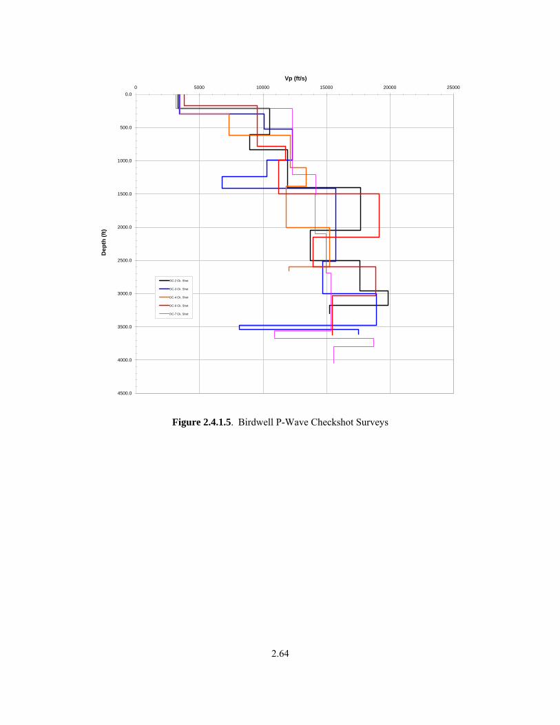
2.64
0.0
500.0
1000.0
1500.0
2000.0
2500.0
3000.0
3500.0
4000.0
4500.0
0 5000 10000 15000 20000 25000
Vp (ft/s)
Dep
th (f
t)
DC-2 Ck. Shot
DC-3 Ck. Shot
DC-4 Ck. Shot
DC-6 Ck. Shot
DC-7 Ck. Shot
Figure 2.4.1.5. Birdwell P-Wave Checkshot Surveys

2.65
0.0
500.0
1000.0
1500.0
2000.0
2500.0
3000.0
3500.0
4000.0
4500.0
0 5000 10000 15000 20000 25000
Vp (ft/s)
Dep
th (f
t)
DC-1 Sonic (re-interpretation)DC-19 Sonic (re-interpretation)DC-20 Sonic (re-interpretation)RRL-2 Sonic (re-interpretation)DC-2 Ck. ShotDC-3 Ck. ShotDC-4 Ck. ShotDC-6 Ck. ShotDC-7 Ck. Shot
Figure 2.4.1.6. Birdwell P-Wave Checkshot Surveys and Reinterpreted Sonic Logs

2.66
0.0
500.0
1000.0
1500.0
2000.0
2500.0
3000.0
3500.0
4000.0
4500.0
0 5000 10000 15000 20000
Vs (ft/s)
Dep
th (f
t)DC-1 Sonic (re-interpretation)DC-19 Sonic (re-interpretation)DC-20 Sonic (re-interpretation)RRL-2 Sonic (re-interpretation)DC-2 Ck. ShotDC-3 Ck. ShotDC-4 Ck. ShotDC-6 Ck. ShotDC-7 Ck. Shot
Figure 2.4.1.7. Inferred Birdwell S-Wave Checkshot Surveys and Reinterpreted Sonic Logs
2.4.2 Vp and Vs in Deep Basalts and Interflow Zones
Although there are many compressional wave borehole logs in the basalts available near the WTP site, no shear wave logs are available. There are two sources of shear wave characterization of the basalts and interflows of the basalts, one from a 1999 proprietary borehole log 60 miles southwest of the WTP site and another from an old 1979 cross-borehole measurement made between boreholes DC-7 and DC-8.

2.67
These measurements are described below to determine the appropriate value for the ratio Vp/Vs for the basalts and interflow zones. Laboratory measurements on small samples from core in some of these boreholes were not considered to be representative of the in situ values, and there was too much uncertainty in how to extrapolate laboratory measurements to depth for this to be useful.
In 1999, a borehole south of the Hanford Site was logged using the Schlumberger Dipole Shear Sonic Imager. This log is proprietary, but information can be derived from it on the ratio of compressional and shear wave velocities, or Vp/Vs. The log was digitized, and the measured values of Vp and Vs are shown in Figure 2.4.2.1 as a function of depth. The logged interval begins in the lower part of the Wanapum Basalt, extends into the Grand Ronde Basalt, and includes the same lava flows present at the Hanford Site and WTP. These flows do not have a significant amount of interbedded sediments, but inter-flow structures, flow tops and bottoms, and other vesicular or fractured zones create velocity reductions in the borehole. This characteristic is typical of the basalt Vp logs available at the Hanford Site and nearer to the WTP and was used to develop a basis for estimating the Vs structure from the Vp data.
The ratio of Vp/Vs is shown in greater detail in Figure 2.4.2.2, along with the value of Poisson’s ratio derived from Vp/Vs. It is apparent that there are some fluctuations in Vp/Vs and Poisson’s ratio that do not appear realistic, even implying a negative Poisson’s ratio for some intervals. Figure 2.4.2.3 shows the Vp/Vs ratio plotted against the value of Vp measured for each depth. These data show relatively small scatter where Vp is high in the massive, largely intact central portions of the basalt flows. In the flow tops and vesicular or altered zones, the scatter in Vp/Vs increases significantly, but there is a trend for decreasing Vp/Vs for decreasing Vp.
The original logs were examined for depth intervals where there appeared to be differences between velocity estimates based on different combinations of receivers, or receivers and sources, on the logging tool. These should give comparable results, although they do measure velocity over different distances or slightly different depth intervals. In areas of rapid change in velocity, the different measurements will diverge naturally, but in many cases it is apparent that the measurements may not be accurate due to poor signals and borehole wall condition. The borehole wall may be broken in weaker interflows and other fractured intervals. A few obvious outliers were removed, and intervals where Poisson’s ratio and Vp/Vs changed abruptly with depth were examined and checked on the basis of whether the different measurements were consistent. The results of this editing are shown in Figure 2.4.2.4, including the measurement points on the Vp and Vs plots. Two significant intervals were completely edited—for example, near depths of 2,200 and 3,100 to 3,200 ft. The resulting Vp/Vs values are now much smoother.
Figure 2.4.2.5 shows an expanded view of Vp and Vs as a function of depth along with the calculated value of Poisson’s ratio. Figure 2.4.2.6 shows the plot of Vp/Vs as a function of Vp for these edited data. The scatter in these data has obviously been decreased significantly; Poisson’s ratio is never near 0 or negative, but several anomalous points remain, with Vp/Vs lows near 2,100 and 2,950 ft and below 3,300 ft and a few highs at 2,400 and 2,950 ft. An examination of the alternative velocity measurements did not indicate a basis for editing these data points.
Another interval where the velocity ratios are low is between the 2,050- and 2,100-ft depths. This interval is actually represented by the Vantage sedimentary interbed, one of the last interbeds present in the deeper basalts. There are only a few points in this interval, but the data indicate that Vp/Vs is reduced, implying

2.68
that Vp is reduced by a greater amount than Vs. This is noted to be the opposite sense of change compared to that found in sediments above the topmost basalt, and these measurements may also be affected by the drilling and measurement processes.
The data from the Vantage interbed interval was removed from the edited data, and the remaining data were fitted using least squares to a linear relationship of Vp/Vs dependent on Vp.
The relationship determined was
Vp/Vs = 1.70 + 6*10-6 Vp.
This linear fit reduced the standard error by only 10%, so the slope is not considered significant. The relationship predicts a Vp/Vs ratio of 1.76, 1.79, and 1.82 for basalt Vp values of 10,000, 15,000, and 20,000, respectively. We have chosen to use a value of 1.79 considering that we have tended to overweight the high-velocity data because of the need to edit data primarily from the slower velocity intervals. The standard error of the value of Vp/Vs is 0.05. This value is supported by the Vp/Vs value of 1.78 developed in earthquake location models that have been used for decades in the region.
A cross-borehole Vp and Vs log (Holosonics 1978) was obtained from two boreholes drilled side by side (DC 7/8, Figure 2.4.1) on the Hanford Site. Logging was performed from 2,875- to 4,000-foot depths. The data from the table in the report were entered into a computer file and edited to exclude any points flagged in the report as inferior, and six additional outliers were removed, leaving 55 points.
In this depth range, the distance between the boreholes changes due to deviation of the boreholes from vertical. This deviation was measured (the report does not state with what instrument; it was likely a gyroscope or tiltmeter), and the distance between the boreholes increased monotonically with depth from 43 to 69 ft (26 ft total change). The distance between the boreholes is critical to the estimation of velocities, and there is clear correlation of Vp and Vs with the distance between the boreholes (and thus also with depth). Figure 2.4.2.7 shows the correlation of Vp with the distance between the two boreholes at depth. (The ramp-like structures in the scattered data are the result of the timing resolution of 0.05 milliseconds.) The values of Vp are near 30,000 fps for the closest borehole separations (at shallowest depths); such velocities are not seen in any other measurement of Vp in basalts. Therefore, it is concluded that both the absolute and relative distances between the two boreholes is not accurately known. The relative distance change between the two boreholes appears to be overestimated by approximately 33% or about 10 ft. The absolute distance error appears to be an additional 10 to 15 ft.
Regardless of this inaccuracy, the ratio of Vp/Vs should not be affected by the errors in the distance between the boreholes (as long as the two waves follow the same path). Figure 2.4.2.8 shows Vp/Vs as a function of borehole separation, and the correlation with distance is removed.
The mean value of Vp/Vs that results from averaging these data is 1.78, with a standard deviation of 0.12. This value of Vp/Vs is in close agreement with the value determined previously from the Schlumberger log, and the use of this Hanford Site information is considered as supporting the values determined with those data.

2.69
Thus, the value of 1.79 for Vp/Vs in the basalts is considered to be an accurate characteristic value for the basalts and will be used to construct the Vs profiles in the site ground motion response model, based on the available measured Vp data.
Figure 2.4.2.1. Compressional and Shear Wave Velocities in Deep Basalts. The ratio Vp/Vs (multiplied by 1000) is shown at left.

2.70
Figure 2.4.2.2. Poisson’s Ratio and Vp/Vs as a Function of Depth in Deep Basalts
Figure 2.4.2.3. Vp/Vs as a Function of Vp in Deep Basalts

2.71
Figure 2.4.2.4. Edited Vp and Vs Data in Deep Basalts. The values for Vp/Vs (multiplied by 1000) are shown at left.
Figure 2.4.2.5. EditedVp/Vs as a Function of Vp in Deep Basalts

2.72
Figure 2.4.2.6. Edited Values of Vp/Vs Plotted as a Function of Vp, and Estimated Relationship Between Vp/Vs and Vp
Figure 2.4.2.7. Correlation of Vp with Cross-Borehole Distance

2.73
Figure 2.4.2.8. Vp/Vs from Cross-Borehole Measurement
2.4.3 Estimates of Vp/Vs in the Interbeds of the Saddle Mountains Basalt Section
Very few compressional wave and no shear wave velocity logs were made in depth intervals that include the Saddle Mountains Basalt and the major interbeds that are present there. The sonic logs that were available did include one from borehole DC-2 (Figure 2.4.1), located approximately 5,000 ft northeast of the WTP site. This sonic log was in several forms, and two of these were used: a computer printout of the borehole log velocity values, and a hard copy of a printed log that had been calibrated by checkshot measurements at DC-2.
One basis for estimating the Vp/Vs ratio in the interbeds is to use the observed Vp/Vs ratios in the Ringold sediments above the topmost basalt. This approach was used previously for the 1996 Geomatrix velocity model. The Vp and Vs measurements were made at the Shear Wave Borehole (or SWVB) logged using the downhole method by Northland/Redpath and the suspension logging method by Geovision. This borehole is 6,000 ft southwest of the WTP site and includes minor differences in the Ringold stratigraphy compared to those expected at the WTP site. Different portions of the Ringold have different Vp/Vs ratios, and they are correlated with the lithology of each unit and on the values of Vp measured in each unit. Vp/Vs in the Ringold itself is not used to calculate Vs in the Ringold because the measured Vs is used. However, the values of Vp/Vs in the Ringold are considered indicative of the appropriate values to use in the four interbeds within the Saddle Mountains Basalt that underlie the Ringold Formation.
The Ringold Formation is confined by 260 ft of Hanford formation and is 280 ft thick at the SWVB. The four interbeds of interest are confined by significantly greater overburdens at the WTP site (see Figure 2.1.3): 440 ft for the Rattlesnake Ridge Interbed, 685 ft for the Selah Interbed, 805 ft for the Cold

2.74
Creek Interbed, and 1,050 ft for the Mabton Interbed. The greater confining pressure is likely to make the relationship between Vp/Vs and Vp or lithology only an approximation or guide to predicting appropriate values of Vs for the interbeds.
The values for Vp/Vs and Poisson’s ratio from the Northland/Redpath measurements and the Geovision measurements within the Ringold Formation are listed in Tables 2.4.3.1 and 2.4.3.2, respectively. The Geovision measurements are shown in Figure 2.4.3.1, and the derived parameters are shown versus depth in Figure 2.4.3.2 and as a function of Vp in Figure 2.4.3.3.
On the plot of Vp/Vs against Vp in Figure 2.4.3.3, it is apparent that there are two clusters of points, one having high Vp and low Vp/Vs, and another having low Vp and high Vp/Vs, with more scatter in Vp/Vs for the latter (low Vp).
Comparing the Vp/Vs ratios in Figure 2.4.3.3, measured from the suspension log in the Ringold Formation, to those measured using the downhole method in Table 2.4.3.1, the fitted equation to the suspension logs results predicts Vp/Vs ratios of 2.98 for Vp of 5,475, and 2.22 for Vp of 9,440. Two different Vp/Vs ratios were observed for Vp of 5,475 because the Vp logs did not detect the lower velocity in the thin Lower Mud unit. Based on the available measurements, a large range (2.0 to 3.0) of Vp/Vs ratio is found for low Vp, but for high Vp, Vp/Vs ratios appear to be better constrained and in the range of 1.8 to 2.2.
Interpreting the suspension logs in the form of a block model over depths where the velocity remains nearly constant results in the velocities shown in Table 2.4.3.2. Table 2.4.3.1. Ringold Vp/Vs and Poisson’s Ratio from Downhole Logging Measurements*
Geologic Unit Depth, ft Vs Vp Vp/Vs Poisson’s
Ratio Ringold Unit E 260 – 390 2730 5475 2.00 0.33 Ringold Lower Mud 390 – 424 1975 5475 2.75 0.42 Ringold Unit A, undifferentiated 424 – 530 4323 9440 2.18 0.37 * Measurements from Table 1 of Northland/Redpath (2004).
Table 2.4.3.2. Ringold Vp/Vs and Poisson’s Ratio from Suspension Logging Measurements*
Geologic Unit Depth, ft Vs Vp Vp/Vs Poisson’s
Ratio Ringold Unit E 363 – 380 2400 7000 2.92 0.43 Ringold Lower Mud 380 – 424 1900 5700 3.00 0.44 Ringold Unit A 424 – 496 5800 10600 1.83 0.29 Ringold Unit A silt 496 – 513 2100 5800 2.76 0.42 Ringold Unit A (cont.) 513 – T.D. N/A * Measurements based on interpretation of Geovision (2004, Figure 4).

2.75
Based on the lithology, Ringold mud or silt have measured Vp/Vs of 2.76 to 3.00, whereas Ringold Unit A has Vp/Vs of 1.83, more characteristic of a rock-like material. Ringold Unit A is a well-cemented conglomerate, so its high velocities and Vp/Vs are consistent with this lithology.
Ringold Unit E was not differentiated from the lower Hanford gravels that overlie it in the Northland/Redpath report. Note that there were not enough data to determine Vp/Vs for the lowest part of Ringold Unit A. Although this is the only part of the Ringold that exists at the WTP site, the Vp/Vs estimates are examined only for possible application to estimating Vs in the sedimentary interbeds within the Saddle Mountains Basalt.
2.4.3.1 Application of Ringold Vp/Vs to the Interbeds
The positions of the four interbeds are shown in Table 2.1.1. They range in thickness from 20 to 115 ft and are from 440 to 1050 ft beneath the surface at the WTP site. The lithology of the interbeds is based on examination of core from boreholes DB-8 and DC-2 (Figure 2.4.1). DC-2 is located approximately 5000 ft northwest of the WTP site, and DB-8, the cored borehole closest to the WTP site, is located 1000 ft northeast. These were cored in the 1980s as part of the Basalt Waste Isolation Project repository study.
Table 2.4.3.3. Lithology of Interbeds from Core Holes near WTP Site
Interbed Name/ WTP Thickness
Borehole DB-8 1,000 ft NE of WTP
Borehole DC-2 5,000 ft NW of WTP
Similar Ringold at SWVB
Rattlesnake Ridge 60 ft
100% siltstone 100% siltstone Unit A siltstone
Selah 20 ft
50% mudstone 50% sandstone
67% mudstone 33% sandstone
Lower mud Unit A siltstone
Cold Creek 95 ft
30% mudstone 70% silt/sandstone
20% siltstone, 70% conglomerate 10%
mudstone
Lower mud* Unit A siltstone*
Mabton 115 ft
100% siltstone 100% siltstone Unit A siltstone
* Based on regional trends and proximity to Borehole DB-8.
Based on the data summarized in Table 2.4.3.3, all of the interbeds are expected to be similar in lithology to the Ringold Lower Mud and Unit A siltstone. Based on Table 2.4.3.2, these units are the low-velocity depth ranges of the Ringold measurements, with Vs measured as 1,900 and 2,100 fps, respectively. If a Vp/Vs value for these layers is applicable in converting the deeper interbed’s Vp to Vs, a value of 2.75 to 3.0 is appropriate. If the composition of the Cold Creek Interbed was more like that at borehole DC-2, the higher velocities and lower Vp/Vs values for Ringold Unit A are more appropriate. Whether a Vp/Vs of 2.75 to 3.0 is appropriate to use at depth is problematic but does represent an extreme case that produces the lowest Vs in the interbeds and thus the strongest impedance contrasts with the intervening basalt layers. Using Vp/Vs, as indicated by Vp, is considered to be a way to compensate for potential differences in lithology and depth of burial. However, based on the scatter in the measurements and the fact that the SWVB was a cased borehole, reliable measurement of Vp/Vs or Poisson’s ratio was not expected by the measurement contractor Geovision (Rob Steller, personal communication, 2004).

2.76
The value of Vp/Vs in the interbeds is considered to be not very well determined. As a result, a range of values was used to determine whether the ground motion response calculations are sensitive to the assessment of Vp/Vs. A range from 1.8 to 2.8 is indicated in the Ringold measurements. However, a reduced range of 2.0 to 2.6 was finally used for the deeper interbed Vs in the ground motion response calculations, as discussed in Section 3.
Figure 2.4.3.1. Vs and Vp as a Function of Depth at the Shear Wave Borehole. See Figure 2.3.4.1.

2.77
Figure 2.4.3.2. Vp/Vs and Poisson’s Ratio as a Function of Depth at the Shear Wave Borehole
Figure 2.4.3.3. Vp/Vs Ratios from Ringold Formation Versus Vp. The regression equation that resulted was Vp/Vs = 4.02 - 0.19*10-3*Vp(fps). The resulting standard error was 0.44 after regression and 0.64 before.

2.78
2.4.4 SASW Vs for Basalts and Interbeds
The SASW Vs profiles through the Hanford and Ringold formations were presented in Section 2.3.5, but the focus of that section was on the sedimentary layers. It was noted there that the measured Vs in the basalt layers was 4,000 to 5,500 fps. These velocities were reached at close to the top-of-basalt depths determined from lithologic logs at nearby boreholes, ranging from 270- to 540-ft depths. The SASW are new measurements that primarily measure Vs rather than Vp. The historical downhole logs discussed in Section 2.4.1 are exclusively measurements of compressional wave Vp rather than the desired Vs. The conversion of the Vp to Vs logs requires knowledge of the ratio Vp/Vs, and this was determined for the basalt layers to be a nearly constant value of 1.79. However, there is substantial uncertainty regarding the value of Vp/Vs in the sedimentary interbeds, and the interbeds often have comparable thicknesses with the Saddle Mountains Basalts with which they alternate. The downhole velocity logs indicate significantly slower velocities in the interbeds compared to the basalts. SASW measurements do not reflect this variability and instead indicate monotonically increasing velocity with depth. This section of the report interprets this difference in characteristics of the basalt velocity structure as determined from downhole and SASW measurements.
A base case model of Vs is developed in Section 2.5 using statistical analysis of the various velocity measurements, Vp/Vs ratios, and layer thicknesses measured from the lithology near the WTP. This model is compared to the SASW profiles surrounding the WTP construction site in Figure 2.4.4.1. (The details of this model are not the same as the final values used in the ground motion response modeling, which is the subject of Section 3.) The SASW profiles to not have the characteristic comb-like structure (alternating high and low velocities) as does the base case model. However, the SASW profiles do appear to represent a reasonable average for these layers.
It is not visually clear how the SASW averages velocities through the basalts and interbeds. Figure 2.4.4.2 compares a calculation of the predicted dispersion curve that would result from modeling the base case velocity model to the measured dispersion curves. The measured dispersion values are fit well with a model that has low-velocity interbeds embedded in the basalts. Therefore, the SASW provides information on the average of the basalts and interbeds. For these cases, with the basalt underlying a significant sediment thickness, the long wavelengths needed to penetrate the sediments ultimately average over 500-ft depth intervals in the deeper basalt and interbed layers.
Figure 2.4.4.3 shows the SASW profile for SASW site 10, which was obtained directly on a basalt outcrop 6 miles to the northwest of the WTP site (see Figure 2.1.7 for location). At this site, the topmost basalt (Elephant Mountain Member) and interbed (Rattlesnake Ridge Interbed) have been removed by erosion, so the top of the stack begins with the more massive basalt called the Pomona Member. Still, there are no velocity inversions imaged in the SASW result. The velocity profile reaches 4,000 fps within 200 ft from the surface. At the approximate depth (550 ft) of the base of the Saddle Mountains Basalt, where the Wanapum Basalt begins, the velocity increases to near 8,000 fps. The Wanapum basalts are not interbedded with sediments, and so it appears that the SASW responds to this with a higher average velocity. This higher basalt velocity is comparable to the base case model average in the Wanapum and deeper basalts.
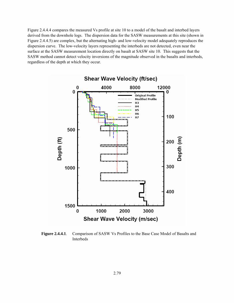
2.79
Figure 2.4.4.4 compares the measured Vs profile at site 10 to a model of the basalt and interbed layers derived from the downhole logs. The dispersion data for the SASW measurements at this site (shown in Figure 2.4.4.5) are complex, but the alternating high- and low-velocity model adequately reproduces the dispersion curve. The low-velocity layers representing the interbeds are not detected, even near the surface at the SASW measurement location directly on basalt at SASW site 10. This suggests that the SASW method cannot detect velocity inversions of the magnitude observed in the basalts and interbeds, regardless of the depth at which they occur.
Figure 2.4.4.1. Comparison of SASW Vs Profiles to the Base Case Model of Basalts and Interbeds

2.80
Figure 2.4.4.2. Comparison of SASW Measured Dispersion to Base Case Model Calculated Dispersion
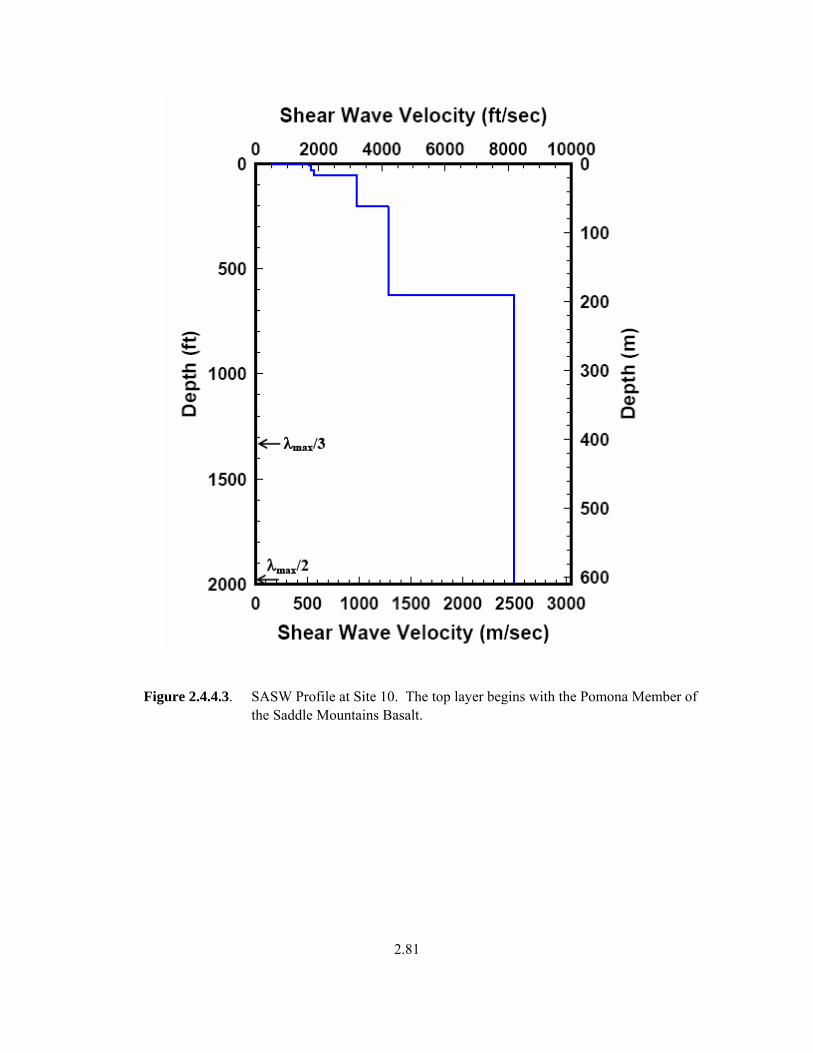
2.81
Figure 2.4.4.3. SASW Profile at Site 10. The top layer begins with the Pomona Member of the Saddle Mountains Basalt.

2.82
Figure 2.4.4.4. Comparison of SASW Profile at Site 10 to Model of Basalts and Low-Velocity Interbed Layers

2.83
Figure 2.4.4.5. Comparison of SASW Dispersion Curve at Site 10 to Model of Basalts
and Low-Velocity Interbed Layers
2.5 Statistical Description of Velocity Models
For the purposes of site response analysis, fractile estimates (16th, 50th, 84th) of the sediment and basalt velocities are required. Each of the measured or inferred S-wave interpretations was subdivided vertically and categorized by sediment type (Hanford or Ringold sediments), shallow basalts and interbeds (Saddle Mountain Basalt) and deep basalts (Wanapum Basalt), based on the available stratigraphy. Because measurements for the deeper sediments and basalts were limited in number and, in some cases, unavailable in the immediate vicinity of the WTP site, all interpretations for a particular measurement type were combined by depth for each of the measurement types. Median, 16th, and 84th percentile velocities of assumed lognormal shear-wave speed were computed for every 1-ft depth interval for each of the measurement types for each of the four geologic conditions:
• Hanford sands and gravels • Ringold Formation • shallow basalts and interbeds • basalts.

2.84
In each of the four geologic conditions, an assessment is made on the consistency of the inferred Vs profile, and, in some cases, the profiles from different techniques are combined. The median 16th, and 84th percentiles were obtained by computing the mean and mean ± one standard deviation of the log of velocity (i.e., assuming the velocities are log-normally distributed).
2.5.1 Hanford Sands and Gravels
Fractile Vs profiles estimates for the seismic cone penetrometer testing (SCPT) at the WTP site are shown in Figure 2.5.1. S-wave model fractile estimates using SASW and downhole logging at the WTP site and vicinity are shown in Figures 2.5.2 and 2.5.3, respectively. A comparison of the fractile estimates is shown in Figure 2.5.4. For the upper 180 ft of the Hanford formation, all three methods produce very similar results showing median profiles smoothly increasing with depth. For depths greater than about 180 ft, the median SASW interpretation is slower relative to the downhole measurements by as much as 350 ft/sec. Although there are few downhole measurements at these depths, this difference is considered real and must be considered as a difference due to the method used (shear wave polarization, profile averaging along SASW lines versus point location at boreholes) or to lateral variation. The four downhole measurements at the WTP site are not co-located with corresponding SASW measurements made around the periphery of the WTP site. If a statistical average is appropriate for handling this difference, Figure 2.5.5 shows the combined S-wave fractile measurements.
2.5.2 Ringold Formation
Fractile estimates of the SASW and downhole Vs interpretations that include the Ringold formation are shown in Figure 2.5.6. For most of the Ringold only one down-hole measurement is available and is generally consistent with the SASW interpretations. Fractile estimates for the combined SASW and down-hole interpretations are shown in Figure 2.5.7.
2.5.3 Shallow Saddle Mountains Basalt and Ellensburg Formation Interbeds
The shallow basalts and interbed Vs profiles are obtained from SASW, and inferred from the Birdwell checkshot surveys and the DC-1 sonic log. The fractile Vs estimates for SASW measurements are shown in Figures 2.5.8. The SASW models did not resolve the interbed structure known to be present in the Saddle Mountains Basalt. The SASW velocities are interpreted to be average models for the Saddle Mountains Basalt and interbed sequence.
Based on sonic log measurements of Vp in the Saddle Mountains and Wanapum basalts, it is expected that a velocity profile for the basalt below the WTP would not be smooth or uniform as these SASW profiles suggest, but would have alternating high and low velocities corresponding to the presence of basalt and interbeds, respectively. The Vp profiles in basalts and interbeds were converted to Vs profiles using a Vp/Vs value of 1.79 for the basalts (Section 2.4.2) and 2.18 for the interbeds. This interbed Vp/Vs was based on the value measured in Ringold Unit A (Table 2.4.3.1). A range of Vp/Vs values from 2.0 to 2.6 was actually used in the site response modeling (Section 3). The fractile Vs profile for the checkshot data in the Saddle Mountains Basalt is shown in Figure 2.5.9.

2.85
Figure 2.5.10 presents a comparison of the SASW and checkshot survey fractile estimates. This comparison suggests that for depths between about 500 and 1,100 ft, the median Vs from the SASW interpretation is about 25% to 35% lower than the median Vs inferred from the checkshot survey (4,700 as compared to 6,200 ft/sec). This difference is considered significant; therefore, these two median models were considered to represent a fundamental uncertainty in models of the Saddle Mountains Basalt and interbeds for the site response evaluation of the WTP.
A sample profile exemplifying the Saddle Mountains Basalt was constructed from the stratigraphic log of DC-2 and the P-wave interpretation derived by Birdwell for that same hole. This profile used two alternative values of Vp/Vs—1.79 and 2.18—for the stratigraphic intervals indicated to be interbeds. The resulting Vs profiles are also shown on Figure 2.5.10 for comparison with the Vs fractile profiles from SASW and checkshot data. The larger Vp/Vs value reduces Vs in the interbeds of the hypothetical model, lowering the average Vs of the Saddle Mountains Basalts and interbeds. This lower average velocity is in better agreement with the SASW data.
2.5.4 Wanapum Basalt
The Wanapum Basalt shear wave velocity profiles are inferred from the Birdwell checkshot and sonic log surveys using a Vp/Vs of 1.79. The re-interpreted sonic and check shot survey fractile estimates for Vs are shown in Figures 2.5.11 and 2.5.12, respectively. Both models are interpreted to be average models for the Wanapum Basalt. A comparison of the fractile estimates of Vs is shown in Figure 2.5.13 and indicates that the two types of surveys can be combined as shown in Figure 2.5.14.
Hanford Soils
0
20
40
60
80
100
120
0 500 1000 1500 2000 2500Vs (ft/sec)
Dep
th (f
t) SCPT medianSCPT 84thSCPT 16th
Figure 2.5.1. Fractile S-Wave Model of WTP Sands and Gravels Based on Seismic Cone Block-Models

2.86
Hanford Soils
0
50
100
150
200
250
300
350
400
450
0 500 1000 1500 2000 2500 3000
Vs (ft/sec)
Dep
th (f
t) sasw-mediansasw-84thsasw-16th
Figure 2.5.2. Fractile S-Wave Model of WTP Vicinity Sands and Gravels Based on SASW Surveys
Hanford Soils
0
50
100
150
200
250
300
0 500 1000 1500 2000 2500 3000Vs (ft/sec)
Dep
th (f
t) DH-medianDH-84thDH-16th
Figure 2.5.3. Fractile S-Wave Model of WTP Vicinity Sands and Gravels Based on Downhole Seismic Surveys
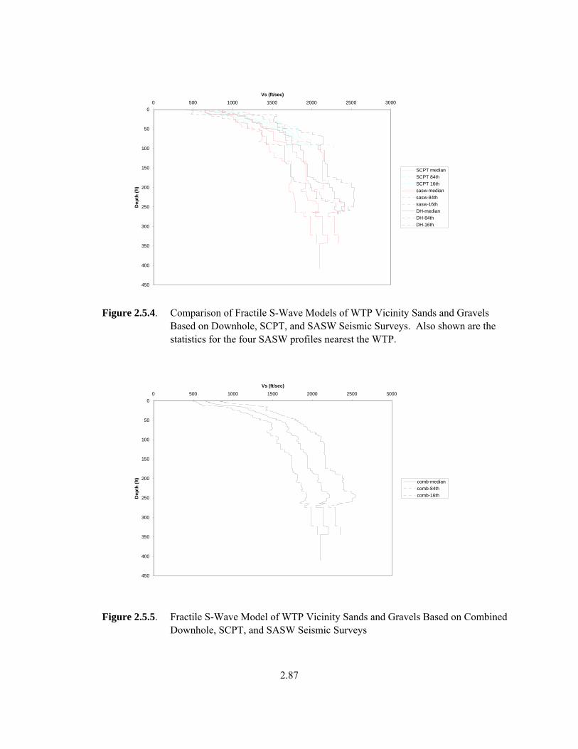
2.87
Hanford Soils
0
50
100
150
200
250
300
350
400
450
0 500 1000 1500 2000 2500 3000
Vs (ft/sec)
Dep
th (f
t)
SCPT medianSCPT 84thSCPT 16thsasw-mediansasw-84thsasw-16thDH-medianDH-84thDH-16th
Figure 2.5.4. Comparison of Fractile S-Wave Models of WTP Vicinity Sands and Gravels Based on Downhole, SCPT, and SASW Seismic Surveys. Also shown are the statistics for the four SASW profiles nearest the WTP.
Hanford Soils
0
50
100
150
200
250
300
350
400
450
0 500 1000 1500 2000 2500 3000Vs (ft/sec)
Dep
th (f
t) comb-mediancomb-84thcomb-16th
Figure 2.5.5. Fractile S-Wave Model of WTP Vicinity Sands and Gravels Based on Combined Downhole, SCPT, and SASW Seismic Surveys

2.88
Figure 2.5.6. Comparison of Fractile S-Wave Models in the Ringold Formation Based on SASW and Downhole Surveys in the Vicinity of the WTP
Ringold
0
100
200
300
400
500
600
0 500 1000 1500 2000 2500 3000 3500 4000 4500 5000
Vs (ft/sec)
Dep
th (f
t) comb-mediancomb-84thcomb-16th
Figure 2.5.7. Fractile S-Wave Model for the Ringold Formation Based on SASW and Downhole Surveys in the Vicinity of the WTP
0
100
200
300
400
500
600
0 1000 2000 3000 4000 5000 6000
Vs (ft/sec)
Depth (ft)sasw-median sasw-84th sasw-16th DH-median DH-84th DH-16th

2.89
Interbeds
0
200
400
600
800
1000
1200
1400
1600
0 1000 2000 3000 4000 5000 6000 7000 8000 9000 10000
Vs (ft/sec)
Dep
th (f
t)sasw-median
sasw-84th
sasw-16th
Figure 2.5.8. Fractile S-Wave Model Based on SASW for the Saddle Mountains Basalt
Saddle Mountain Basalts
0
200
400
600
800
1000
1200
1400
1600
0 1000 2000 3000 4000 5000 6000 7000 8000 9000 10000
Vs (ft/sec)
Dep
th (f
t)
chksht-median
chksht-84th
chksht-16th
Figure 2.5.9. Fractile S-Wave Model Based on Checkshot Surveys for the Saddle Mountains Basalt

2.90
Interbeds
0
200
400
600
800
1000
1200
1400
1600
0 1000 2000 3000 4000 5000 6000 7000 8000 9000 10000
Vs (ft/sec)
Dep
th (f
t)
sasw-mediansasw-84thsasw-16thchksht-medianchksht-84thchksht-16thDC-1/2 hypotheticalVs(sonic/calib/ringold)
Figure 2.5.10. Combined Plot of Fractile S-Wave Models for SASW and Checkshot Surveys for the Saddle Mountains Basalt. Also shown is the DC-1 inferred model for two hypothetical values of Vp/Vs.
Basalts
0
500
1000
1500
2000
2500
3000
3500
4000
4500
0 2000 4000 6000 8000 10000 12000
Vs (ft/sec)
Dep
th (f
t) sonic-mediansonic-84thsonic-16th
Figure 2.5.11. Fractile Basalt S-Wave Model Based on P-Wave Sonic Logs in Deep Basalts

2.91
Basalts
0
500
1000
1500
2000
2500
3000
3500
4000
4500
0 2000 4000 6000 8000 10000 12000
Vs (ft/sec)
Dep
th (f
t) chksht-medianchksht-84thchksht-16th
Figure 2.5.12. Fractile Basalt S-Wave Model Based on P-Wave Checkshot Surveys in Deep Basalts
Basalts
0
500
1000
1500
2000
2500
3000
3500
4000
4500
0 2000 4000 6000 8000 10000 12000
Vs (ft/sec)
Dep
th (f
t)
sonic-mediansonic-84thsonic-16thchksht-medianchksht-84thchksht-16th
Figure 2.5.13. Fractile Basalt S-Wave Models Based on Reinterpreted P-Wave Sonic Logs and P-Wave Checkshot Surveys
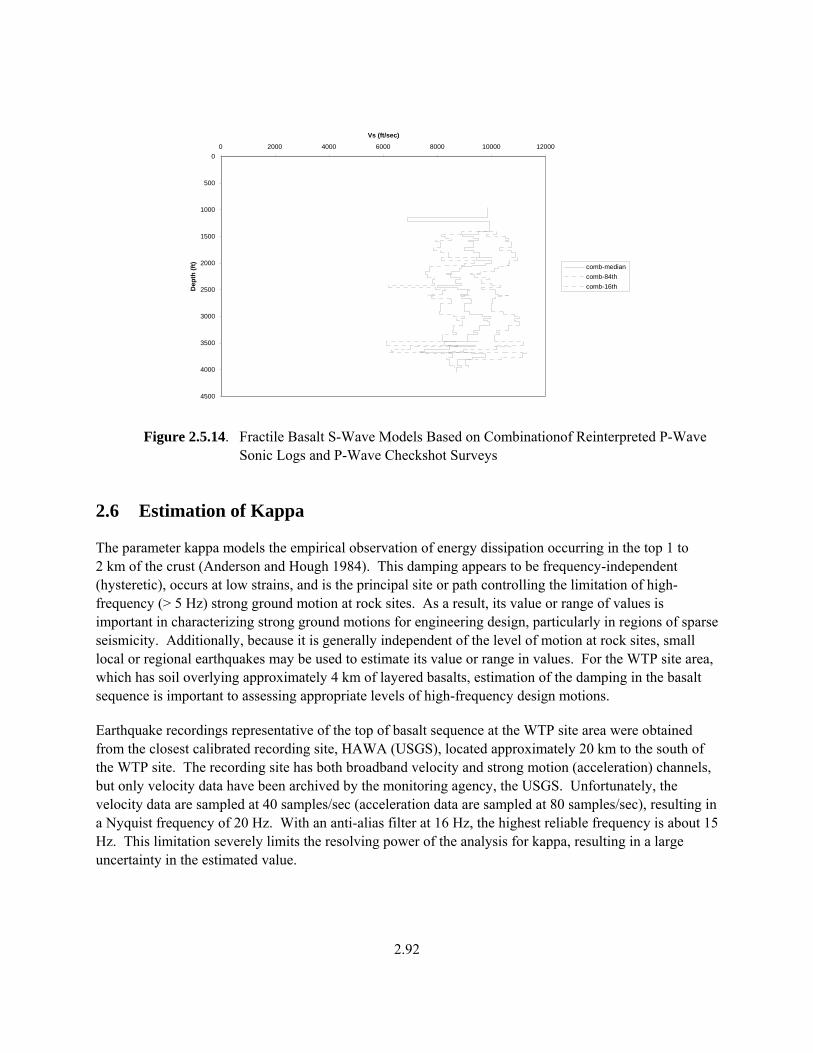
2.92
Basalts
0
500
1000
1500
2000
2500
3000
3500
4000
4500
0 2000 4000 6000 8000 10000 12000
Vs (ft/sec)
Dep
th (f
t) comb-mediancomb-84thcomb-16th
Figure 2.5.14. Fractile Basalt S-Wave Models Based on Combinationof Reinterpreted P-Wave Sonic Logs and P-Wave Checkshot Surveys
2.6 Estimation of Kappa
The parameter kappa models the empirical observation of energy dissipation occurring in the top 1 to 2 km of the crust (Anderson and Hough 1984). This damping appears to be frequency-independent (hysteretic), occurs at low strains, and is the principal site or path controlling the limitation of high-frequency (> 5 Hz) strong ground motion at rock sites. As a result, its value or range of values is important in characterizing strong ground motions for engineering design, particularly in regions of sparse seismicity. Additionally, because it is generally independent of the level of motion at rock sites, small local or regional earthquakes may be used to estimate its value or range in values. For the WTP site area, which has soil overlying approximately 4 km of layered basalts, estimation of the damping in the basalt sequence is important to assessing appropriate levels of high-frequency design motions.
Earthquake recordings representative of the top of basalt sequence at the WTP site area were obtained from the closest calibrated recording site, HAWA (USGS), located approximately 20 km to the south of the WTP site. The recording site has both broadband velocity and strong motion (acceleration) channels, but only velocity data have been archived by the monitoring agency, the USGS. Unfortunately, the velocity data are sampled at 40 samples/sec (acceleration data are sampled at 80 samples/sec), resulting in a Nyquist frequency of 20 Hz. With an anti-alias filter at 16 Hz, the highest reliable frequency is about 15 Hz. This limitation severely limits the resolving power of the analysis for kappa, resulting in a large uncertainty in the estimated value.

2.93
The initial selected data consisted of recordings of 21 earthquakes, with magnitudes ranging from 2.0 to 3.3, and source-to-station distances from 10 to 80 km from the location of the HAWA station. A screening of waveforms for good signal/noise ratios and clear onset of the shear wave arrivals indicated that only the 9 deeper events (greater than 8 km depth) were useable. An additional 16 deep earthquakes with magnitudes ranging from 1.5 to 2.0 with distances from 10 to 50 km also were screened. Of these 25 deep earthquakes, 10 were selected that were judged to provide the best estimate of kappa.
An inversion process was used to estimate kappa in which the earthquake source, path, and site parameters are obtained by using a nonlinear least-squares fit to the Fourier amplitude spectra using the point-source model (Boore 1983; EPRI 1993). The useable bandwidth for each amplitude spectrum computed from recordings was selected based upon visual examination. In no cases did the bandwidth extend beyond the anti-alias filter corner frequencies (approximately 16 Hz). The inversion scheme treats multiple earthquakes and sites simultaneously with the common crustal path damping parameter Q(f). The parameter covariance matrix is examined to determine which parameters may be resolved for each data set. Asymptotic standard errors are computed at the final iteration. The five parameters that may be determined from the data are kappa (site-specific attenuation), Q0 (the value of Q for f equal to 1 Hz), and η (frequency-dependent path Q model), M, and corner frequency (stress drop). The procedure uses the Levenberg-Marquardt algorithm (Press et al. 1986). Crustal profile amplification is accommodated in the inversion scheme by incorporating the appropriate mean transfer functions (source depth to surface) in estimating the surface spectra.
To reduce the potential for non-uniqueness inherent in inversion results, a suite of starting models is employed. The final set of parameters is selected based upon a visual inspection of the model fit to the Fourier amplitude spectrum, the chi-square values, and the parameter covariance matrix.
The stress drop is calculated from the moment and corner frequency using the relation
31
oc M44.8
f ⎟⎟⎠
⎞⎜⎜⎝
⎛⋅σ∆β=
The inversions are done on log amplitude spectra (vector average of the two horizontal components), because strong ground motion data appear to be log normally distributed. This is consistent with the model being represented as a product (rather than sum) of models (EPRI 1993). The inversion bandwidth is magnitude dependent, generally extending to lower frequency with increasing magnitudes or closer distance. The low-frequency limit is based on visual examination of each average spectrum. The high-frequency limit was set at 15 Hz based on the data sampling interval.
Results of the inversions for kappa are listed in Table 2.6.1 along with starting values, and the fits to the spectra are shown in Figure 2.6.1. The best-estimate kappa value is 0.024 sec and was obtained using starting values of either 0.02 sec or 0.04 sec. Due to the severe limitations in bandwidth at high frequency (15 Hz), the stress drops, which are unusually small, are not considered reliable. In addition, the narrow bandwidth precluded determination of crustal Q(f), so it was fixed at 500(f)0.6. As a consequence, because some of the distances are fairly large (86 km, Table 2.6.1), the kappa value must be considered to be conditional on this Q(f) model.
(2.1)

2.94
Although the inversion kappa value of 0.024 sec is independent of starting values of 0.020 sec and 0.040 sec indicating reasonable uniqueness (for this bandwidth), the uncertainty in this best estimate (mean value) is large. Based on previous experience with this inversion process, the estimated uncertainty in the mean kappa value is likely about 1.3. The range in mean kappa then is from about 0.018 sec to 0.031 sec.
Table 2.6.1. Results of Kappa Inversion from Earthquake Spectra
Magnitude Stress Drop, bars Input Value* Final Value Input Value Final Value
Hypocentral Distance, km
1.49 2.03 0.1 0.25 45 3.25 2.94 0.1 7.46 46 2.55 2.31 0.1 1.48 86 1.51 1.96 0.1 2.32 44 2.63 2.47 0.1 9.45 66 3.17 2.51 0.1 3.05 81 1.63 2.02 0.1 4.81 45 2.63 2.54 0.1 2.17 69 1.81 2.23 0.1 2.95 42 1.58 2.14 0.1 2.21 36
* Input magnitudes from coda length Initial κ = 0.02 sec, 0.04 sec Final κ = 0.024 sec

2.95
Figure 2.6.1. Fourier Amplitude Spectra for the Data (Average Horizontal Component) Initial Model Calculations and Final Model Calculations. The measured spectra are shown as the solid lines, and the initial and fitted spectra are shown as dashed and dashed-dotted lines, respectively.

3.1
3.0 Ground Motion Response Modeling
The geological and geotechnical data developed in Section 2 are used here to evaluate the response of the WTP site structure to earthquake ground motion. Ground motions were selected based on the probabilistic seismic hazard study in 1996. The seismic source information has not changed since 1996, and the use of more recent attenuation relationships is not expected to change the calculated hazard significantly (BNFL 1999). The site response modeling is conducted in the same manner as was done for the previous sensitivity analyses performed by Geomatrix Consultants, Inc. (Geomatrix 2003).
3.1 Modeling Issues and Uncertainties
A well-founded, consistent model was established for the Hanford formation. The formation thickness and lithology (gravel versus sand) are well known. Recent borehole measurements (including four directly beneath the WTP structures) produce shear wave velocity profiles that are consistent with this lithology. The SASW data confirmed the velocity structure in the Hanford formation. All data were statistically examined to determine the coefficient of variation or “sigma” used to randomize the earthquake response models.
There is much larger uncertainty in the characterization of the Ringold Formation beneath the WTP site. Only one good Vs measurement was available, from the SWVB. Three primary factors introduce uncertainty into the model for this layer—the location of the Vs measurement, 6,000 ft from the WTP site; the variable, eroded, thickness of the Ringold Formation across the area due to the paleochannel; and the complex lithology of the Ringold Formation (muds, silts, gravels). Thin low-velocity sections of the Ringold Formation were found in various locations using the suspension logging method, which has higher resolution than the downhole method, but the average velocities important to the modeling were in agreement. SASW data from near the SWVB are approximately consistent with the downhole logging. The SASW from the profiles measured at the WTP site show variable and generally lower velocities in the Ringold—2,500 fps—compared to the 4,000-fps average at the SWVB location.
There are large uncertainties also in the characterization of the Saddle Mountains Basalt and the interbedded Ellensburg Formation sediments. The available velocity data consist of one Vp sonic log in addition to several checkshot Vp averages. The checkshot averages were used to calibrate this log, and then values of Vp/Vs were used to convert these Vp logs to Vs. This results in a significant change to the velocities in the shallowest basalt and interbed layers from the velocity model used in the 1996 study.
The Vp/Vs ratio for deep Wanapum and Grande Ronde Basalts was found to be very well determined. Although it is assumed that this same Vp/Vs applies to the shallower Saddle Mountains Basalt, this assumption is judged to be accurate.
There were no data on Vp/Vs of the interbedded Ellensburg Formation sediments, and this remains a source of large uncertainty in the model. Vp/Vs ratios were determined from the logs in the SWVB and compared to the known lithology there, to estimate the appropriate Vp/Vs value to estimate Vs in the interbeds.

3.2
The SASW results in the basalt do not detect the interbeds. Modeling of dispersion curves that include low-velocity zones demonstrates that the method averages through such structures and so does not support the conclusion that the SASW models in basalt can be used directly to define the velocity structure in this environment.
Differences in shallow crustal attenuation between California and Hanford are an additional source of uncertainty in the prediction of ground motion spectra. The limited data to determine the shallow crustal attenuation parameter kappa, or κ, results in significant uncertainty in ground motion response at high frequency.
Uncertainties in the site response model are developed using a logic tree approach. The results of the relative site response analyses, conducted using the alternative site characterizations defined in the logic tree, are used to show the sensitivity of the ground motion response in terms of relative amplification factors to different assumptions about the model parameters. These amplification factors were used to construct a conservative assessment of the relative response of the WTP site as compared to California deep soil sites. California soil sites are representative of the empirical attenuation models used in the 1996 probabilistic seismic hazard analysis. These conservative relative amplification factors were used to develop new design spectra for the WTP site.
3.2 Logic Tree Approach to Hanford Waste Treatment Plant Ground Motion Amplification Factors
Examination of seismic and geologic data collected in the vicinity of the WTP site at Hanford has produced a model of the subsurface physical properties of the site. However, several significant uncertainties in some of the actual properties at the site still exist, due to limited data or inherent variability. A range of values for these properties has been selected to determine the sensitivity of the amplification factors to these properties. The approach uses a conventional logic tree, with branches that define the distribution of site properties and weights that reflect the relative likelihood that the parameters on the individual logic tree branches represent the actual properties at the WTP site (Figure 3.2.1 and Table 3.2.1). The site response model that results from each path through the logic tree is used to calculate the relative site ground motion response to earthquake ground motions representative of the site hazard. Based on the quality and consistency of the available data, weights for each of the branch points were selected by the working group named in the Acknowledgments section of this report.
Several elements of the model indicate that there are significant amplifications of ground motion response by the WTP Hanford site structure relative to the response of California deep soil sites representative of the ground motion attenuation relationships used to develop the original seismic design. It was also found that ground motion response is sensitive to two poorly known parameters of the model—the crustal attenuation parameter kappa and the Vs in the interbeds within the Saddle Mountains Basalt.
The stratigraphic elements of the site response model are shown in Figure 3.2.2. Thicknesses of the soil layers are accurately determined from numerous boreholes in the surrounding area, and the thicknesses of the deeper basalt and interbeds are not observed to have significant variability over a broader surrounding area. Densities in Figure 3.2.2 were obtained from historical data in nearby boreholes using borehole gravimeter data.

3.3
3.2.1 Hanford Sands and Gravels
The uppermost layers in the model are the Hanford Sands and Gravels. The Vs profile for these layers is well known at the WTP site and is not an element of the logic tree. The Vs data on which these profiles are based include
• seismic cone penetration testing (SCPT) within the WTP site (26 profiles in the upper 100 ft) • downhole within the WTP site (4 profiles to between 260 and 270 ft) • downhole surrounding the WTP site (4 profiles to between 200 and 260 ft, 1 profile to 530 ft into
the Ringold unit below) • spectral analysis of surface waves (SASW) (4 along the boundary of the WTP site, 5 additional in
the surrounding area).
The Vs model for the Hanford Sands and Gravels is considered to be sufficiently well known that alternatives are not included in the logic diagram. The strain-dependent properties (modulus reduction and damping) of the Hanford Sands were assessed by Shannon & Wilson for the 200 East and 200 West Areas and were found to be consistent with a generic set of relationships published by EPRI (1993). The strain-dependent properties of the Hanford Gravels are more uncertain, and two alternative sets of parameters (Rollins et al. [1998] and Silva et al. [1998] for Peninsula Range sites), were included in the site response model logic tree.
3.2.2 Ringold Formation
The sedimentary layer below the Hanford Sands and Gravels and the basalt/interbed stack is the Ringold Formation. The Ringold Formation consists of a variety of sand, mud, and gravel layers that are variable across the area of the WTP. Figure 3.2.3 shows the thickness of the Ringold Formation in the area of the WTP. Of note is an erosional “paleochannel” that has cut through the Ringold Formation in the area.
The Vs data for the Ringold Formation are more limited than those for the Hanford Formation and include
• downhole and suspension logs (in one borehole 530 ft through the Ringold Formation) • SASW measurements (four along boundary of WTP site, five additional in surrounding area).
The variability of the thickness and velocities measured in the Ringold Formation present one of the significant uncertainties in the response model. Downhole measurements made in the 530-ft-deep borehole showed that the Ringold Formation had Vs ranging from 2,700 to 4,300 fps, depending upon the composition (sands and muds versus gravels) of the corresponding depth range in the Ringold Formation. These data will be examined further when the logic tree weighting process is described below.
Higher-resolution suspension logging measurements in the same borehole had Vs ranging from lows near 2,000 fps and highs in the 5,000- to 6,000-fps range, with the higher Vs in the gravels. In the deepest 90 ft of the borehole, the downhole measurements indicate an average Vs of 4,300 fps. In the suspension logs, the Vs varied from 2,000 to 6,000 fps, but the average Vs was comparable to the downhole result.
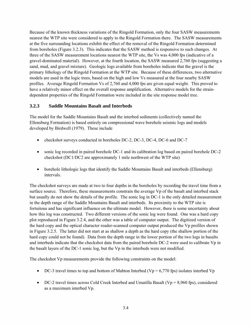
3.4
Because of the known thickness variations of the Ringold Formation, only the four SASW measurements nearest the WTP site were considered to apply to the Ringold Formation there. The SASW measurements at the five surrounding locations exhibit the effect of the removal of the Ringold Formation determined from boreholes (Figure 3.2.3). This indicates that the SASW method is responsive to such changes. At three of the SASW measurement locations nearest the WTP site, the Vs was 4,000 fps (indicative of a gravel-dominated material). However, at the fourth location, the SASW measured 2,760 fps (suggesting a sand, mud, and gravel mixture). Geologic logs available from boreholes indicate that the gravel is the primary lithology of the Ringold Formation at the WTP site. Because of these differences, two alternative models are used in the logic trees, based on the high and low Vs measured at the four nearby SASW profiles. Average Ringold Formation Vs of 2,760 and 4,000 fps are given equal weight. This proved to have a relatively minor effect on the overall response amplification. Alternative models for the strain-dependent properties of the Ringold Formation were included in the site response model tree.
3.2.3 Saddle Mountains Basalt and Interbeds
The model for the Saddle Mountains Basalt and the interbed sediments (collectively named the Ellensburg Formation) is based entirely on compressional wave borehole seismic logs and models developed by Birdwell (1979). These include
• checkshot surveys conducted in boreholes DC-2, DC-3, DC-4, DC-6 and DC-7 • sonic log recorded in paired borehole DC-1 and its calibration log based on paired borehole DC-2
checkshot (DC1/DC2 are approximately 1 mile northwest of the WTP site) • borehole lithologic logs that identify the Saddle Mountains Basalt and interbeds (Ellensburg)
intervals.
The checkshot surveys are made at two to four depths in the boreholes by recording the travel time from a surface source. Therefore, these measurements constrain the average Vp of the basalt and interbed stack but usually do not show the details of the profile. The sonic log in DC-1 is the only detailed measurement in the depth range of the Saddle Mountains Basalt and interbeds. Its proximity to the WTP site is fortuitous and has significant influence on the ultimate model. However, there is some uncertainty about how this log was constructed. Two different versions of the sonic log were found. One was a hard copy plot reproduced in Figure 3.2.4, and the other was a table of computer output. The digitized version of the hard copy and the optical character reader-scanned computer output produced the Vp profiles shown in Figure 3.2.5. The latter did not start at as shallow a depth as the hard copy (the shallow portion of the hard copy could not be found). Data from the depth range in the lower portion of the two logs in basalts and interbeds indicate that the checkshot data from the paired borehole DC-2 were used to calibrate Vp in the basalt layers of the DC-1 sonic log, but the Vp in the interbeds were not modified.
The checkshot Vp measurements provide the following constraints on the model:
• DC-3 travel times to top and bottom of Mabton Interbed (Vp = 6,770 fps) isolates interbed Vp • DC-2 travel times across Cold Creek Interbed and Umatilla Basalt (Vp = 8,960 fps), considered
as a maximum interbed Vp.

3.5
The checkshot average Vp through multiple basalt and interflow layers reach highs of 12,000 fps, as shown in Figure 3.2.6. Below the Saddle Mountains Basalt and interbeds, the highest Vp values are in the range of 15,000 to 20,000 fps. These deeper Wanapum and Grande Ronde Basalts (see Figure 3.2.1) do not have significant interbeds, although flow structures near the top of each flow still produce thin low Vp intervals. The deeper basalts are included in the response models and form one of the contributions to the modeling of the crustal attenuation term kappa.
The working group chose the following ranges of Vp for the Saddle Mountains Basalt and the interbedded sediments composing the Ellensburg Formation, due to the limited Vp data available.
For the Saddle Mountains Basalt:
• Range on Vp for the Saddle Mountain Basalt was judged from the borehole DC-1 calibrated sonic log.
o Basalt Vp is a nominal 80 µsec/ft (Vp = 12,500 fps). o Uncertainty in basalt Vp is nominally 10 µsec/ft (Vp = 14,400 and 11,100 fps).
• Vp was measured in lower two basalt members (Umatilla and Esquatzel) and the interbeds beneath (Cold Creek and Mabton).
o The same Vp and uncertainty range were applied to upper two basalt layers (Elephant Mountain and Pomona).
For the Ellensburg Formation interbeds:
• Collective average Vp for interbeds is nominally 130 µsec/ft (Vp = 7,690 fps). • Low Vp measured in interbeds is 170 µsec/ft (Vp = 5,880 fps). • High Vp measured in interbeds is 110 µsec/ft (Vp = 9,100 fps).
Nominal values representing the low, middle, and high values were used in the logic tree shown in Figure 3.2.1. The logic tree therefore represents nine combinations of basalt and interbed Vp. Figure 3.2.7 compares the calculated average Vp from the nine models to the statistical median and 16th and 84th percentiles derived from the checkshot data.
Weights in the logic tree for the Vp in basalt were assigned as follows. A large weight (0.5) was given to the central estimate of 12,500 fps. A slightly larger weight (0.3) was assigned to the higher Vp limit of 14,400 fps than the weight (0.2) assigned to the lower Vp limit of 11,100 fps. The higher weight was given to the higher Vp to accommodate the uncertainty in the way the checkshot calibration was originally performed.
Weights in the logic tree for the Vp in interbeds were based on limiting the average Vp of the resulting basalt and interbed stack to that represented by the checkshot statistics. The central value of interbed Vp is generally given the highest weight. Weights for the higher or lower interbed Vp were based on the resulting average Vp of the basalt and interbed stack, with a preference toward maintaining this average within the checkshot statistics. For example, interbed Vp weights, associated with the low-Vp basalt branch, were chosen to be relatively higher for the higher interbed Vp branch because the average Vp of the basalt and interbed stack was closer to the range of the checkshot average Vp. The distribution of the resulting average Vp from the logic model is shown in Figure 3.2.8.

3.6
Figure 3.2.1. Logic Tree for Hanford Waste Treatment Plant Seismic Response Model
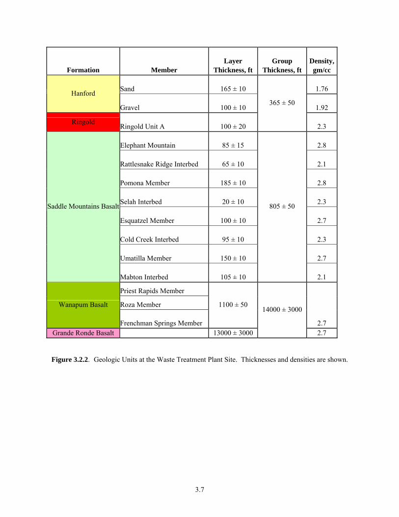
3.7
Formation Member Layer
Thickness, ft Group
Thickness, ft
Density,gm/cc
Sand 165 ± 10
1.76 Hanford
Gravel 100 ± 10
1.92
Ringold Ringold Unit A 100 ± 20
365 ± 50
2.3
Elephant Mountain 85 ± 15
2.8
Rattlesnake Ridge Interbed 65 ± 10
2.1
Pomona Member 185 ± 10
2.8
Selah Interbed 20 ± 10
2.3
Esquatzel Member 100 ± 10
2.7
Cold Creek Interbed 95 ± 10
2.3
Umatilla Member 150 ± 10
2.7
Saddle Mountains Basalt
Mabton Interbed 105 ± 10
805 ± 50
2.1
Priest Rapids Member
Roza Member Wanapum Basalt
Frenchman Springs Member
1100 ± 50
2.7 Grande Ronde Basalt 13000 ± 3000
14000 ± 3000
2.7
Figure 3.2.2. Geologic Units at the Waste Treatment Plant Site. Thicknesses and densities are shown.

3.8
Figure 3.2.3. Thickness Variation of Ringold Formation. The brown shaded area shows where the Ringold sediments have been eroded through. Additional thickness of Hanford formation replaces them in these areas.

3.9
Figure 3.2.4. Original Calibrated Sonic Log from DC-1. This log was digitized and is compared to a computer output version of the log in Figure 3.2.5.

3.10
0
200
400
600
800
1000
1200
1400
1600
1800
2000
0 5000 10000 15000 20000 25000 30000Vp (ft/sec)
Dep
th (f
t)
WELL # DC-1DC-2 (scanned)
Sediments
Figure 3.2.5. Comparison of the Tabulated Sonic Log for DC-1 and the Calibrated Sonic Log Using the DC-2 Checkshot Data

3.11
0.0
500.0
1000.0
1500.0
2000.0
2500.0
3000.0
3500.0
4000.0
4500.0
0 5000 10000 15000 20000 25000
Vp (ft/s)
Dep
th (f
t)
DC-2 Ck. Shot
DC-3 Ck. Shot
DC-4 Ck. Shot
DC-6 Ck. Shot
DC-7 Ck. Shot
Figure 3.2.6. Comparison of the Five Checkshot Velocity Profiles in the Vicinity of the Waste Treatment Plant. Note the isolated low velocity in the interbed near 1,300 ft for the DC-3 profile (blue) and the low velocity in a single interbed-basalt combination at 700 ft in the DC-2 profile (black).

3.12
0
200
400
600
800
1000
1200
1400
1600
0 2000 4000 6000 8000 10000 12000 14000 16000 18000
Vp (ft/sec)
Dep
th (f
t)
b11.1,i6 (.04)b12.5,i6 (.1)b11.1,i7.5 (.06)b14.4,i6 (.09)b12.5,i7.5 (.2)b11.1,i9 (.1)b14.4,i7.5 (.15)b12.5,i9 (.2)b14.4,i9 (.06)chksht-medianchksht-84thchksht-16thVp(sonic/calib)
Figure 3.2.7. Comparison of the Median and 16th and 84th Percentiles of the Checkshot Vp with the Average Vp Resulting from the Nine Logic Tree Models. The central branch of the logic tree model with Vp 12,500 fps basalt and 7,500 fps interbeds is shown as the black line. Basalt and interbed Vp from Table 3.2.1 label the Vp averages, including the weights used in the logic tree.
0
0.05
0.1
0.15
0.2
0.25
0.3
0.35
7500-8000
8000-8500
8500-9000
9000-9500
9500-10000
10000-10500
10500-11000
11000-11500
11500-12000
Average Vp
Figure 3.2.8. Distribution of Weights of Average Vp in the Basalt and Interbeds

3.13
3.2.4 Construction of the Vs Model
An important step in the construction of a response model is to convert the Vp model described above into a Vs model. For the basalts, there were sufficient in situ data from regional boreholes sources to establish that the Vp/Vs ratio was 1.79 within the basalts. Therefore, no uncertainty in this conversion was included in the logic tree. For the interbeds, there are no direct data for estimating Vs from what limited Vp data are available, and the uncertainty in Vp/Vs was incorporated in the logic tree.
Because there are no direct data on Vp/Vs for the interbeds, two sources of information are used. The downhole and suspension Vp and Vs logs that were made in the Ringold Formation at depths from 360 ft to 530 ft provide a useful analogue. In addition, many of the SASW Vs surveys provide a measure of the average Vs in the basalt and interbed stack; this measure can be used to constrain Vs in the interbeds.
In the Ringold Formation, the sand and mud layers had lower Vp and Vs than the gravel layers. The reduction in Vs was larger in the sand and mud layers than the reduction for Vp, resulting in a higher value of Vp/Vs for these layers compared to the gravel layers. Borehole cores of the interbeds from nearby boreholes indicate a composition dominated by sands and muds, indicating low Vs. The suspension logs provided numerous detailed measurements of Vp and Vs in the Ringold Formation, and the ratio Vp/Vs is shown as a function of Vp in Figure 3.2.9. The values of Vp/Vs near 1.8 are correlated with Vp values higher than 10,000 fps and are representative of the gravel units of the Ringold Formation. The downhole logs in the Ringold Formation provided three additional measurements of Vp/Vs—2.0, 2.18, and 2.75, where the corresponding Vp were 5,500, 9,500, and 5,500 fps—but these do not indicate a similar correlation between Vp/Vs and Vp. The average Vp/Vs of these three downhole measurements is 2.3.
The logic tree was constructed initially with nearly the full range of possible Vp/Vs values observed in the Ringold Formation (1.8 to 2.8). Subsequent examination of the resulting Vs distribution and the sensitivity of the ground motion response to this parameter led to a reduced range from 2.0 to 2.6, maintaining the central value of 2.3. A low Vp/Vs value of 1.8 is indicative of a gravel- or basalt rock-like material that is not indicated by either the core samples (sands and muds) or Vp measurements (all well below 10,000 fps) in the interbeds. A high Vp/Vs value of 2.8 corresponds to the minimum Vp in the Ringold Formation in the logic tree. The scatter in the suspension Vp/Vs may indicate unreliable or possibly biased measurements of Vp/Vs. A maximum Vp/Vs value of 2.6 is considered to be more representative of the central range of Vp measured in the sonic log in the interbeds. In addition, the Vp/Vs value of 2.8 found in the Ringold sands and muds might not be representative of the deeper interbeds, and it indicated Vs values lower than were expected. The reduced range is not considered to require changes in the weights, which were assessed based on comparing the computed average Vs of the basalt and interbed stack from the resulting velocities to the average Vs measured in the deeper parts of the SASW profiles, as described below.
The SASW measurements provide a smoothed average of the Saddle Mountains Basalt and interbeds. Figure 3.2.10 shows the four nearest SASW profiles in comparison to the central velocity profile defined in the logic tree. The calculated dispersion curve for an approximation to the central logic tree model (basalt Vs of 7,000 fps, interbed Vs of 3,200 fps; see Table 3.2.1) is superimposed on the measured dispersion curves in Figure 3.2.11. It is preferable to compare the velocity profiles defined in the logic tree by comparing the resulting dispersion curves to the measured dispersion curves as in Figure 3.2.11.

3.14
However, it was judged appropriate to compare the average Vs resulting from the logic tree to the velocity profile statistics estimated from the SASW measurements.
Figures 3.2.12a, 3.2.12b, and 3.2.12c show the depth-averaged (through the basalt and interbed thicknesses) Vs of the velocity models defined in the logic tree for the three chosen values of Vp/Vs (2.0, 2.3, and 2.6). These are also compared to the median and 16th and 84th percentiles calculated from the entire SASW data set. Weights on the values of Vp/Vs were chosen to produce an average Vs that was in the statistical range of the SASW measurements. For the logic tree branches associated with the 11,000-fps and 12,500-fps Vp basalt (Vs 6,200 fps and 7,000 fps), the highest weight of 0.5 was assigned to the interbed Vp/Vs branch that resulted in an interbed Vs between 3,000 fps and 3,500 fps. Weights were progressively lower for alternative values of Vp/Vs in the interbeds outside this range. The highly weighted branches result in average Vs through the basalt interbed stack near 4,500 fps to 5,000 fps. For the logic tree branches associated with the highest Vp (14,400 fps), weights were chosen that produced a lower preferred Vs (below 3,000 fps) using the higher two Vp/Vs ratios where possible. For two of the three interbed Vp branches, Vp/Vs ratios are never large enough to reduce the average Vs of the basalt and interbed stack to the SASW range.
The distribution of average Vs that results from the logic tree is shown in Figure 3.2.13. The central peak is in the range of 4,500 to 5,000 fps in agreement with the SASW measurements. The distribution of average Vs in the basalt interbed stack is skewed to higher Vs than measured by the SASW method. Some of the higher average Vs result from the upper limit of Vp in the basalts. Overall, as shown in Figures 3.2.12a through 3.2.12c, the higher values of Vp/Vs (2.3 and 2.6) produce a better fit to the SASW average than does a Vp/Vs of 2.0. The weighting scheme is conservative in its effect on the response modeling. The interbed Vs distribution in the logic tree model is not low enough to reproduce the average Vs from the SASW measurements, indicating that the Vs contrasts between the basalts and interbeds are underestimated on average, relative to the SASW Vs measurements.
Figure 3.2.9. Velocity Ratio Vp/Vs Versus Vp in the Ringold Compared to the Range of Vp in the
Interbed Logic Tree

3.15
Figure 3.2.10. Comparison of Velocity Profiles from SASW Measurements to the Central Element of the Logic Tree Model
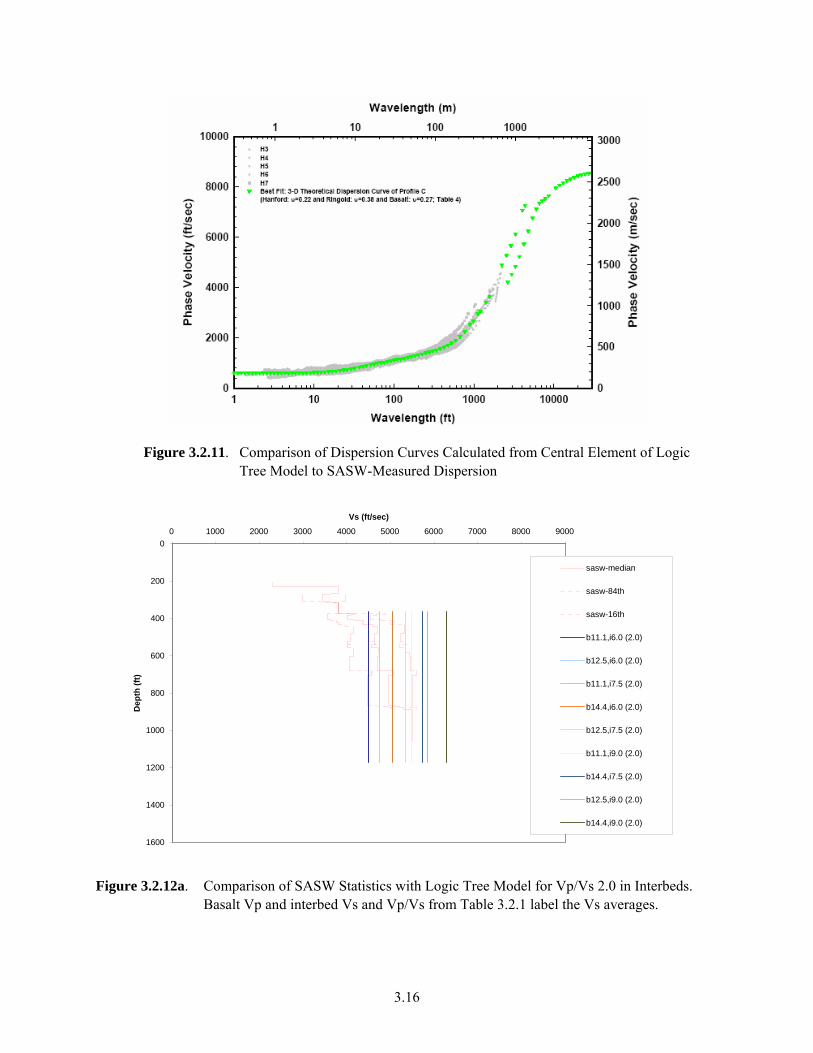
3.16
Figure 3.2.11. Comparison of Dispersion Curves Calculated from Central Element of Logic Tree Model to SASW-Measured Dispersion
0
200
400
600
800
1000
1200
1400
1600
0 1000 2000 3000 4000 5000 6000 7000 8000 9000
Vs (ft/sec)
Dep
th (f
t)
sasw-median
sasw-84th
sasw-16th
b11.1,i6.0 (2.0)
b12.5,i6.0 (2.0)
b11.1,i7.5 (2.0)
b14.4,i6.0 (2.0)
b12.5,i7.5 (2.0)
b11.1,i9.0 (2.0)
b14.4,i7.5 (2.0)
b12.5,i9.0 (2.0)
b14.4,i9.0 (2.0)
Figure 3.2.12a. Comparison of SASW Statistics with Logic Tree Model for Vp/Vs 2.0 in Interbeds. Basalt Vp and interbed Vs and Vp/Vs from Table 3.2.1 label the Vs averages.

3.17
0
200
400
600
800
1000
1200
1400
1600
0 1000 2000 3000 4000 5000 6000 7000 8000 9000
Vs (ft/sec)
Dep
th (f
t)sasw-median
sasw-84th
sasw-16th
b11.1,i6.0 (2.3)
b12.5,i6.0 (2.3)
b14.4,i6.0 (2.3)
b11.1,i7.5 (2.3)
b12.5,i7.5 (2.3)
b11.1,i9.0 (2.3)
b14.4,i7.5 (2.3)
b12.5,i9.0 (2.3)
b14.4,i9.0 (2.3)
Figure 3.2.12b. Comparison of SASW Statistics with Logic Tree Model for Vp/Vs 2.3 in Interbeds
0
200
400
600
800
1000
1200
1400
1600
0 1000 2000 3000 4000 5000 6000 7000 8000 9000
Vs (ft/sec)
Dep
th (f
t)
sasw-median
sasw-84th
sasw-16th
b11.1,i6.0 (2.6)
b12.5,i6.0 (2.6)
b14.4,i6.0 (2.6)
b11.1,i7.5 (2.6)
b12.5,i7.5 (2.6)
b11.1,i9.0 (2.6)
b14.4,i7.5 (2.6)
b12.5,i9.0 (2.6)
b14.4,i9.0 (2.6)
Figure 3.2.12c. Comparison of SASW Statistics with Logic Tree Model for Vp/Vs 2.6 in Interbeds

3.18
0
0.050.1
0.15
0.20.25
0.3
0.35
0.40.45
0.5
3000-3500
3500-4000
4000-4500
4500-5000
5000-5500
5500-6000
6000-6500
6500-7000
Average Vs
Figure 3.2.13. Distribution of Average Vs in Saddle Mountains Basalt and Interbeds Resulting from Logic Tree Weighting
Table 3.2.1. Saddle Mountains Basalt Sequence Velocity Models
Saddle Mt Basalt Vp,
fps
Saddle Mt Interbed Vp, fps
Interbed Vp/Vs Ratio
Saddle Mt Basalt Vs,
fps
Saddle Mt Interbed Vs,
fps
Scenario Weight
11100 6000 2.0 6201 3000 0.020
11100 6000 2.3 6201 2609 0.012
11100 6000 2.6 6201 2308 0.008
11100 7500 2.0 6201 3750 0.015
11100 7500 2.3 6201 3261 0.030
11100 7500 2.6 6201 2885 0.015
11100 9000 2.0 6201 4500 0.020
11100 9000 2.3 6201 3913 0.030
11100 9000 2.6 6201 3462 0.050
12500 6000 2.0 6983 3000 0.050
12500 6000 2.3 6983 2609 0.030
12500 6000 2.6 6983 2308 0.020
12500 7500 2.0 6983 3750 0.040
12500 7500 2.3 6983 3261 0.100

3.19
Table 3.2.1. (continued)
Saddle Mt Basalt Vp,
fps
Saddle Mt Interbed Vp, fps
Interbed Vp/Vs Ratio
Saddle Mt Basalt Vs,
fps
Saddle Mt Interbed Vs,
fps
Scenario Weight
12500 7500 2.6 6983 2885 0.060
12500 9000 2.0 6983 4500 0.040
12500 9000 2.3 6983 3913 0.060
12500 9000 2.6 6983 3462 0.100
14400 6000 2.0 8045 3000 0.0225
14400 6000 2.3 8045 2609 0.045
14400 6000 2.6 8045 2308 0.0225
14400 7500 2.0 8045 3750 0.030
14400 7500 2.3 8045 3261 0.045
14400 7500 2.6 8045 2885 0.075
14400 9000 2.0 8045 4500 0.015
14400 9000 2.3 8045 3913 0.015
14400 9000 2.6 8045 3462 0.030
3.3 Development of Relative Amplification Functions
3.3.1 Approach
The 1996 probabilistic seismic hazard assessment (PSHA) for the Hanford Site (Geomatrix 1996) was conducted using empirical ground motion models developed from data recorded on soil sites primarily in California. The appropriateness of these attenuation models to the subsurface conditions at Hanford was evaluated at that time by performing a relative amplification study. Site response analyses were conducted to compute the response of California soil sites typical of those represented in the empirical strong motion data and to compute the response of Hanford sites. The ratio of the computed surface response spectra (Hanford/California soil) provides a frequency-dependent relative amplification function (RAF). The RAF is a measure of the need to adjust the empirical California soil site ground motion models for use in the PSHA at Hanford. At that time, it was concluded that the RAF was sufficiently close to unity such that the empirical California soil ground motion models could be used without adjustment.

3.20
As described above, the project has developed an updated characterization of the site conditions at Hanford that is specific to the WTP. The relative amplification study was repeated to evaluate the appropriate RAF for the WTP-specific site conditions for the 2,000-year return period motion. All spectral calculations are performed for 5% spectral damping.
3.3.2 Analysis Inputs
Figure 3.3.1 compares the median shear wave velocity profile representative of California soil sites to the median shear wave velocity profile developed for the WTP site. The velocity profiles are extended to a depth of 3 km (9,800 ft) where the shear wave velocities at Hanford and California become comparable. The transition from soil to rock in California, shown at 1,000 ft in Figure 3.3.1, was randomized to lie between 100 and 1,000 ft in the analysis to reflect the variability in soil depth across the strong motion databases used to develop the empirical attenuation relationships. Figure 3.3.2 shows the upper 4,000 ft of these velocity profiles. The velocity in the California soils is somewhat lower than that in the WTP soils. The velocities in the shallow crustal rocks in California begin at about 3,000 fps and show a continuous increase to approximately 10,000 fps at a depth of 10,000 ft. At the WTP site, the upper crustal rocks consist of basalts, with the topmost unit—the Saddle Mountains Basalt sequence—consisting of alternating layers of basalt and interbedded sediments. The rock velocities at the WTP site start out much higher than those in California but show only a small increase with depth. The higher-velocity soils at Hanford produce a somewhat higher response than the California soils. This is offset by the velocity contrasts in the basalt-interbed sequence, which reflects energy downward. The value of sigma (standard deviation for the natural log of shear wave velocity), used to randomize the velocity profiles, are based on a site-specific model for a footprint area developed at Savannah River (H Area) (Silva et al. 1998). It was adopted for the WTP site because the statistical analysis (Section 2.5) of the limited data indicated similar levels for the sigma values. In the Savannah River H Area model, sigma is 0.26 at the surface, decreasing to about 0.15 at a depth of 50 ft and then to about 0.12 for depths below 100 ft. Because the upper ~14 ft of soil at the WTP site have been replaced by backfill, the Savannah River sigmas of ~0.26 were reduced to 0.1 to reflect placement of engineered fill. The California value of sigma of 0.36 is based on the model for generic soil sites from Silva et al. (1998).
Shown on Figures 3.3.1 and 3.3.2 are the differences between the updated velocity model for the WTP site and the base case model for Hanford used in the 1996 study. The WTP updated velocity profile has a thinner soil deposit (365 ft compared to 500 ft) and slower velocities in the Saddle Mountains Basalt (~7,000 ± 1000 fps compared to ~10,000 fps) than was assumed in the 1996 study.
The relative amplification analyses use as input a set of 16 time histories (8 two-component recordings) recorded on California rock sites in earthquakes representative of the dominant contributor to the hazard at the WTP site (M ~6, R < 20 km). The geometric mean of the response spectra for the recorded motions is shown by the blue curve on Figure 3.3.3. These time histories were deconvolved to a depth of 3 km through randomized velocity models for California rock sites. The resulting time histories contain spurious high-frequency motion above 20 Hz, as indicated by the orange curve on Figure 3.3.3. A theoretical shape for the response spectra of rock motions at this crustal depth was obtained using the stochastic ground motion model. This spectral shape (the green curve on Figure 3.3.3) was used to adjust the high-frequency content of the deconvolved motions to remove the spurious high frequencies.

3.21
The relative amplification analyses were conducted using the computer program SHAKE (Schnabel et al. 1972). The soils (top 100 to 1,000 ft in California, top 365 ft at the WTP site) were modeled using equivalent-linear representations of the strain-dependent modulus and damping. Appropriate sets of modulus reduction and damping relationships were used for these materials. Below these depths, the materials (rock in California, basalts and interbeds at the WTP site) were treated as a linear medium (no modulus reduction or damping increase with increasing strain). The amount of damping in the linear materials was estimated from the ground motion parameter kappa (κ). Parameter κ represents a measure of the decay in Fourier amplitude of ground motions with increasing frequency due to energy absorption in the shallow crust. It is related to material damping, ξ, by the relationship
HVS
2κξ =
where H is the thickness of the layer with shear wave velocity VS. By assigning a total value of kappa to the shallow crustal rocks and assuming that damping is inversely proportional to velocity (the model used in the 1996 study), the value of damping in the individual rock layers is obtained. The value of kappa appropriate for California rocks has been estimated from empirical studies to be 0.04 sec (the units are 1/frequency). The value of kappa appropriate for the basalts underlying the Hanford Site was estimated to be in the range of 0.018 to 0.031 sec from a set of rock site recordings obtained to the southwest of the WTP site. Kappa represents the total shallow crustal damping. For the WTP site, there is a significant damping effect (wave reflection and scattering) due to the large velocity contrasts in the Saddle Mountains Basalt/Interbed sequence that are not generally present in California shallow crustal rocks. Figure 3.3.4 shows the relationship between the ratio of basalt to interbed velocities and the effective scattering κ produced by the velocity contrasts. The material damping in the shallow crustal rocks at the WTP site was estimated by first subtracting the scattering kappa (Figure 3.3.4) from the total kappa and then using the remainder to apportion damping based on the velocity of the individual layers. This process was used to maintain the total estimated crustal damping to be consistent with the empirically measured values for all of the alternative velocity models.
3.3.3 Results
The relative response analyses were conducted by generating 30 realizations of representative profiles for California and 30 realizations of each WTP profile. The response of each profile was computed using the 16 input time histories, producing a total of 480 surface response spectra. The geometric mean of these spectra was then computed to obtain the representative surface motions. The geometric mean is used because the intent is to compare the response of the WTP site to California in order to evaluate the need to adjust the California empirical ground motion models. These empirical models are defined in terms of the geometric mean (mean log) of ground motion amplitude recorded on soil sites.
The left-hand plot on Figure 3.3.5 shows examples of the surface response spectra for the California soil sites and three of the velocity models for the WTP site. The right-hand plot shows the corresponding response spectral ratios (WTP/California).
Figures 3.3.6 through 3.3.8 show the sensitivity of the computed response spectral ratios to alternative parameters of the WTP site response model. The left-hand plot of Figure 3.3.6 shows the effect of interbed velocity holding the basalt velocity constant. The right-hand plot shows the effect of total kappa. Variation of these two parameters produces the largest effects on the relative site response. Figure 3.3.7

3.22
shows the effect of the alternative Ringold velocities and alternative sets of soil modulus reduction and damping curves, and Figure 3.3.8 shows the effect of the alternative velocities for the Saddle Mountains Basalt. These parameters have much less effect on the relative site response.
Figure 3.3.9 shows the distribution of response spectral ratios computed using the alternative site response model parameters defined in the revised site response model logic tree (Figure 3.2.1). The results show a consistent amplification near 2 Hz that varies little among the alternative models and amplification above 4 Hz that is strongly dependent on the alternative model parameters, principally interbed velocity and kappa.
The contributions to the range of response result shown in Figure 3.3.9 from each branch of the logic tree are shown in Figures 3.3.10 through 3.3.15. Each of the plots shows the effect of the stated assessments on the mean amplification within the context of the overall uncertainty, as indicated by the percentile curves that were shown in Figure 3.3.9. Figure 3.3.10 shows the strong effect of kappa on the high frequencies, approaching the 84th percentile. Figure 3.3.11 shows there is little effect from the alternative Vs in the logic model for the Ringold Formation, and Figure 3.3.12 shows there is little effect from the alternative models for modulus reduction and damping in the Hanford formation and Ringold Formation. The contributions from basalt Vp, interbed Vp, and interbed Vp/Vs, shown in Figures 3.3.13, 3.3.14, and 3.3.15, respectively, are interrelated as these parameters produce the Vs contrast between the basalt and interbed layers. However, variation of the two parameters for the interbeds has a greater effect on the response variation than does variation in Vp for the basalts.
0
1000
2000
3000
4000
5000
6000
7000
8000
9000
10000
0 2000 4000 6000 8000 10000 12000 14000
Shear Wave Velocity (fps)
Dep
th (f
t)
California Soil Site
1996 Model
Example2004/2005 Model
Figure 3.3.1. Shear Wave Velocity Profiles for California Soil Sites, Waste Treatment Plant Site, and 1996 Hanford Model

3.23
0
500
1000
1500
2000
2500
3000
3500
4000
0 2000 4000 6000 8000 10000 12000 14000
Shear Wave Velocity (fps)
Dep
th (f
t)
California Soil Site
1996 Model
Example 2004/2005Model
Figure 3.3.2. Upper 4,000 feet of Shear Wave Velocity Profiles for California Soil Sites, Waste Treatment Plant Site, and 1996 Hanford Model
0.01
0.1
1
10
0.1 1 10 100
Frequency
Spec
tral
Acc
eler
atio
n
Recorded California Rock
Deconvolved Motions
Stochastic 3 km motions
Modified Deconvolved Motions
Figure 3.3.3. Geometric Mean Response Spectra for Rock Motions Used in Relative Amplification Analysis

3.24
0.000
0.002
0.004
0.006
0.008
0.010
0.012
0 1 2 3 4
Vs basalt/Vs interbeds
Scat
terin
g K
appa
Basalt Vs 6201
Basalt Vs 6983
Basalt Vs 8045
Figure 3.3.4. Relationship Between Basalt/Interbed Velocity Ratio and Effective Scattering Kappa for the Saddle Mountains Basalt Sequence
Example Spectral Ratios
0.4
0.5
0.6
0.7
0.8
0.9
1.0
1.1
1.2
1.3
1.4
0.1 1 10 100
Frequency (Hz)
Spec
tral
Rat
io
HG23M, IB Vs 2143
HG26M, IB Vs 2679
HG29M, IB Vs 3214
Example Statistical Spectra
0.00
0.10
0.20
0.30
0.40
0.50
0.60
0.70
0.80
0.1 1 10 100
Frequency (Hz)
Spec
tral
Acc
eler
atio
n (g
Calif Soil
HG23M, IB Vs 2143
HG26M, IB Vs 2679
HG29M, IB Vs 3214
Figure 3.3.5. Sample Surface Response Spectra and Spectral Ratios
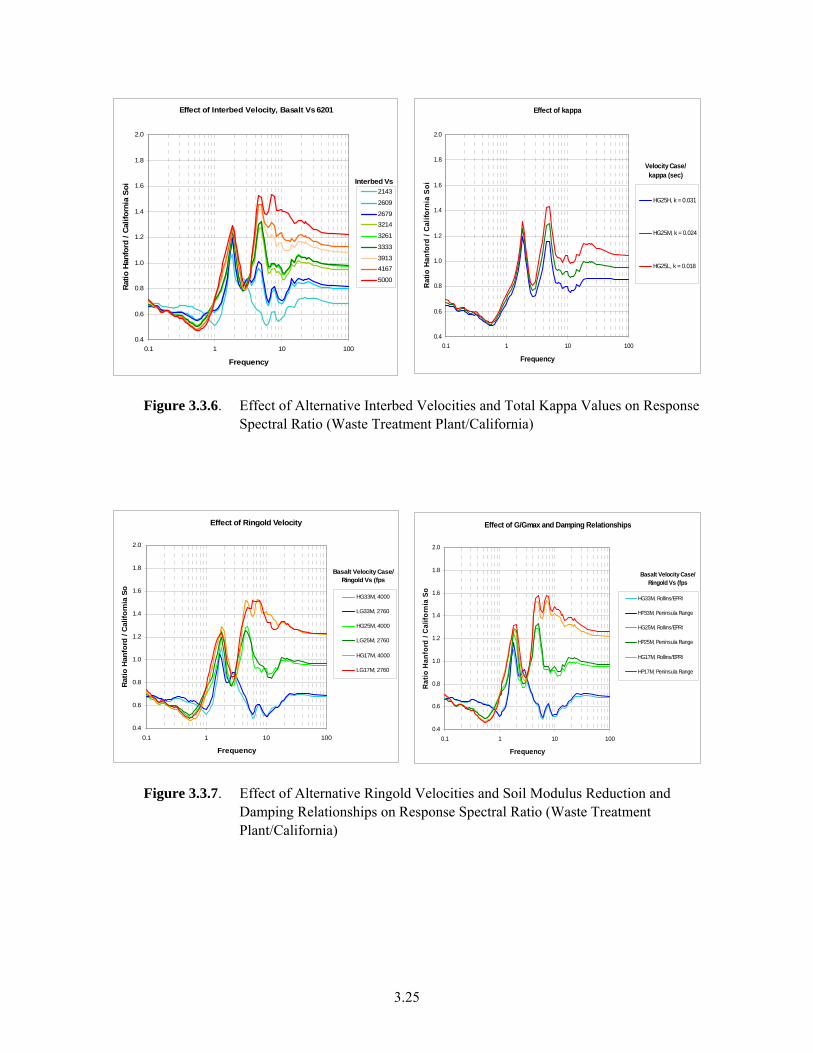
3.25
Effect of Interbed Velocity, Basalt Vs 6201
0.4
0.6
0.8
1.0
1.2
1.4
1.6
1.8
2.0
0.1 1 10 100
Frequency
Ratio
Han
ford
/ Ca
lifor
nia
Soi
2143
2609
26793214
3261
3333
39134167
5000
Interbed Vs
Effect of kappa
0.4
0.6
0.8
1.0
1.2
1.4
1.6
1.8
2.0
0.1 1 10 100
Frequency
Rat
io H
anfo
rd /
Calif
orni
a So
i
HG25H, k = 0.031
HG25M, k = 0.024
HG25L, k = 0.018
Velocity Case/kappa (sec)
Figure 3.3.6. Effect of Alternative Interbed Velocities and Total Kappa Values on Response Spectral Ratio (Waste Treatment Plant/California)
Effect of Ringold Velocity
0.4
0.6
0.8
1.0
1.2
1.4
1.6
1.8
2.0
0.1 1 10 100
Frequency
Rat
io H
anfo
rd /
Cal
iforn
ia S
o
HG33M, 4000
LG33M, 2760
HG25M, 4000
LG25M, 2760
HG17M, 4000
LG17M, 2760
Basalt Velocity Case/Ringold Vs (fps
Effect of G/Gmax and Damping Relationships
0.4
0.6
0.8
1.0
1.2
1.4
1.6
1.8
2.0
0.1 1 10 100
Frequency
Rat
io H
anfo
rd /
Cal
iforn
ia S
o
HG33M, Rollins/EPRI
HP33M, Peninsula Range
HG25M, Rollins/EPRI
HP25M, Peninsula Range
HG17M, Rollins/EPRI
HP17M, Peninsula Range
Basalt Velocity Case/Ringold Vs (fps
Figure 3.3.7. Effect of Alternative Ringold Velocities and Soil Modulus Reduction and Damping Relationships on Response Spectral Ratio (Waste Treatment Plant/California)

3.26
Effect of Basalt Velocity
0.4
0.6
0.8
1.0
1.2
1.4
1.6
1.8
2.0
0.1 1 10 100
Frequency
Ratio
Han
ford
/ Ca
lifor
nia
Soil
6201
6983
8045
Basalt Vs
Figure 3.3.8. Effect of Alternative Saddle Mountains Basalt Velocities on Response Spectral Ratio (Waste Treatment Plant/California)
0.4
0.6
0.8
1.0
1.2
1.4
1.6
1.8
2.0
0.1 1 10 100
Frequency
Rat
io H
anfo
rd /
Cal
iforn
ia S
oil
mean
minimum
0.05
0.1584
0.5
0.8416
0.95
maximum
Figure 3.3.9. Distribution of Relative Site Response (response spectral ratio Waste Treatment Plant/California) Computed Using Site Response Model Logic Tree
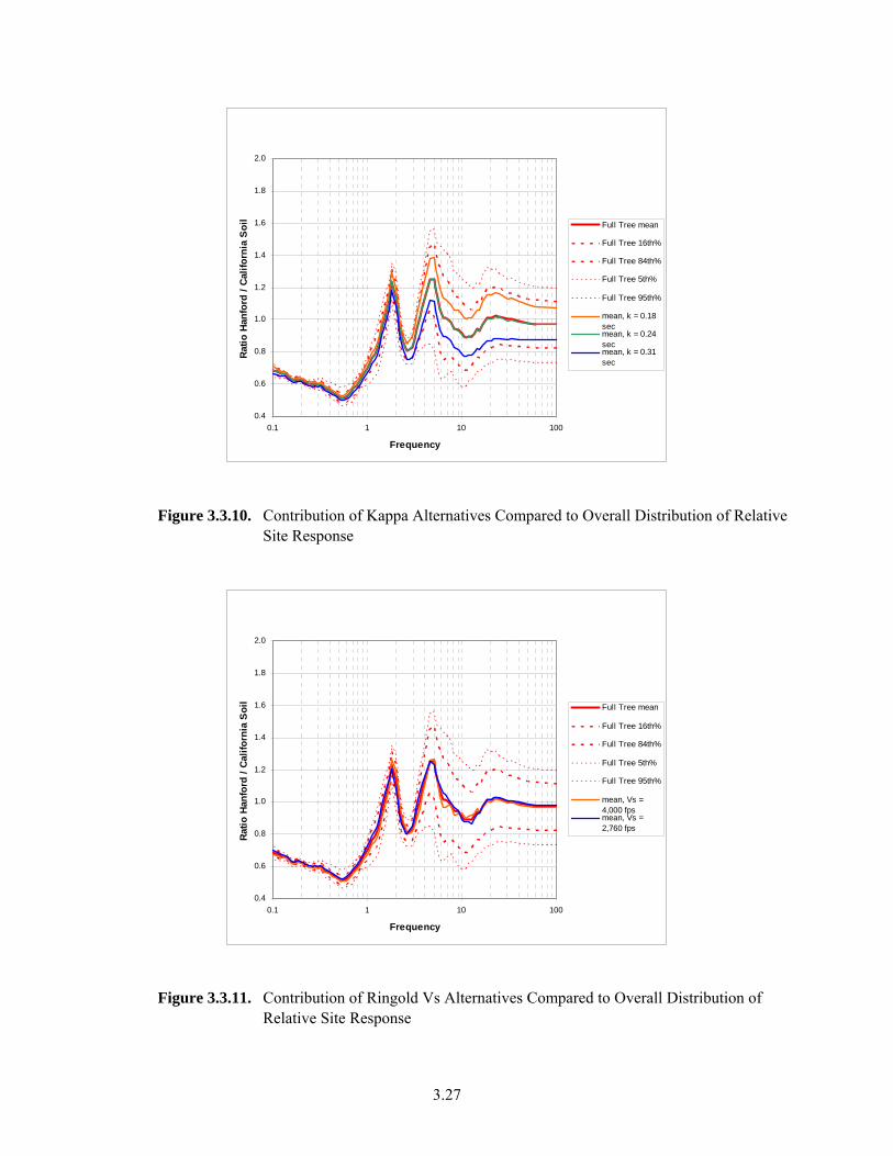
3.27
0.4
0.6
0.8
1.0
1.2
1.4
1.6
1.8
2.0
0.1 1 10 100
Frequency
Ratio
Han
ford
/ Ca
lifor
nia
Soi
l
Full Tree mean
Full Tree 16th%
Full Tree 84th%
Full Tree 5th%
Full Tree 95th%
mean, k = 0.18secmean, k = 0.24secmean, k = 0.31sec
Figure 3.3.10. Contribution of Kappa Alternatives Compared to Overall Distribution of Relative Site Response
0.4
0.6
0.8
1.0
1.2
1.4
1.6
1.8
2.0
0.1 1 10 100
Frequency
Ratio
Han
ford
/ Ca
lifor
nia
Soi
l
Full Tree mean
Full Tree 16th%
Full Tree 84th%
Full Tree 5th%
Full Tree 95th%
mean, Vs =4,000 fpsmean, Vs =2,760 fps
Figure 3.3.11. Contribution of Ringold Vs Alternatives Compared to Overall Distribution of Relative Site Response

3.28
0.4
0.6
0.8
1.0
1.2
1.4
1.6
1.8
2.0
0.1 1 10 100
Frequency
Ratio
Han
ford
/ Ca
lifor
nia
Soil Full Tree mean
Full Tree 16th%
Full Tree 84th%
Full Tree 5th%
Full Tree 95th%
mean, Rollins /EPRImean, PeninsulaRanges
Figure 3.3.12. Contribution of Soil Modulus Reduction and Damping Model Alternatives Compared to Overall Distribution of Relative Site Response
0.4
0.6
0.8
1.0
1.2
1.4
1.6
1.8
2.0
0.1 1 10 100
Frequency
Ratio
Han
ford
/ Ca
lifor
nia
Soil Full Tree mean
Full Tree 16th%
Full Tree 84th%
Full Tree 5th%
Full Tree 95th%
mean, Vp =11,100 fpsmean, Vp =12,500 fpsmean, Vp =14,400 fps
Figure 3.3.13. Contribution of Basalt Vp Alternatives Compared to Overall Distribution of Relative Site Response

3.29
0.4
0.6
0.8
1.0
1.2
1.4
1.6
1.8
2.0
0.1 1 10 100
Frequency
Ratio
Han
ford
/ Ca
lifor
nia
Soi
l
Full Tree mean
Full Tree 16th%
Full Tree 84th%
Full Tree 5th%
Full Tree 95th%
mean, Vp =6,000 fpsmean, Vp =7,500 fpsmean, Vp =9,000 fps
Figure 3.3.14. Contribution of Interbed Vp Alternatives Compared to Overall Distribution of Relative Site Response
0.4
0.6
0.8
1.0
1.2
1.4
1.6
1.8
2.0
0.1 1 10 100
Frequency
Rat
io H
anfo
rd /
Cal
iforn
ia S
oil
Full Tree mean
Full Tree 16th%
Full Tree 84th%
Full Tree 5th%
Full Tree 95th%
mean, Vp/Vs = 2.0
mean, Vp/Vs = 2.3
mean, Vp/Vs = 2.6
Figure 3.3.15. Contribution of Interbed VpVs Alternatives Compared to Overall Distribution of Relative Site Response

3.30
3.4 Derivation of Design Response Spectrum and Frequency-Dependent Relative Amplification Function
This section presents a description of the process used to arrive at a frequency-dependent relative amplification function (RAF) of the WTP site with respect to the empirical California deep soil profile, and to apply this RAF to the current design response spectrum (DRS) to arrive at an interim DRS that can be used to continue the WTP design process in the near term. This interim DRS is an approximation expected to be conservative for application to the facility design.
The process used to develop the RAF makes use of the logic tree results described in Section 3.3. Aleatory variability is accounted for in the site response process by using multiple input time histories and randomizing individual site profiles in determining the site response in each of the subsets of the logic tree. Epistemic uncertainty was accounted for in the process of combining subset responses of the logic tree process. For conservatism in the final design recommendation, the 84th percentile results from the full logic tree were used to guide the final selection of the RAF as well as enveloping the mean responses from individual subsets of the logic tree that were found to lead to higher estimates of the RAF.
Various subsets of logic tree elements also were used in the development of the design recommendation. These combinations generally led to the conclusion that the 84th percentile from the logic tree represented a conservative envelope of the range of the mean results. Therefore, the 84th percentile from the logic tree was chosen to guide the development of the design recommendation. Figure 3.4.1 compares the 84th percentile results from the full data set with the means from several subsets of interest that were felt to be conservative indicators of the expected WTP site response. The subsets considered are the RAF maxima from the interbed Vp/Vs ratio (Vp/Vs of 2.0), the Case 8 mean (Vs of interbeds at 3,913 fps), and the low-kappa case. The 84th percentile from the full data set is somewhat higher than the subset means. This result shows that the 84th percentile RAF from the full logic tree reflects a reasonably conservative estimate of the RAF. The 84th percentile from the logic tree was therefore chosen to guide the development of the design recommendation.
Figure 3.4.2 shows the original 1996 (black line) 5% damped horizontal design response spectrum. That spectrum was then scaled by the 84th percentile frequency-dependent RAF from the full logic tree result to obtain a conservative estimate of the horizontal response spectrum (red line) appropriate for the WTP site. This spectrum was then broadened (green line) at the peak to arrive at the recommended horizontal design response spectrum for the WTP site that conservatively accounts for the differences between the WTP site and the California deep soil profile associated with the attenuation models used in the original UHS development.
The sharp peak of the recommended spectrum (red curve of Figure 3.4.2) is at 5 Hz. The spectral broadening process was accomplished by extending the peak on the low-frequency side about 30% to about 3.85 Hz and about 15% on the high-frequency side to about 5.75 Hz. For higher frequencies, the spectrum was then extended linearly (in log-log space) to a frequency of 12 Hz. The conservatism in the higher frequencies above 12 Hz was found to be significant because the logic tree results indicated that the higher-mode responses of the subsets of the logic tree yielded a dip in the spectra at these frequencies.
The design response spectra calculations presented above are for the horizontal ground motion. In order to obtain corresponding design spectra for vertical ground motion, the ratio of vertical to horizontal (V/H)

3.31
5% damped response spectra was used. The 1996 V/H ratios were derived based on hazard calculations performed using only the Abrahamson and Silva (1995, 1997) and Campbell (1994) attenuation relationships, which included parameters for both vertical and horizontal motions. Recent work (Bozorgnia and Campbell 2004) has indicated that there are changes to the V/H ratios derived from updates to the Campbell attenuation relationships published by Campbell and Bozorgnia (2003). The effect of these updated relationships on the V/H ratios was examined by computing the median response for earthquakes of approximately magnitude 6, at distances of 10, 20, and 30 km, appropriate to the dominant hazard identified in the 1996 probabilistic model. The average of the V/H ratios computed using the Abrahamson and Silva (1995, 1997) and Campbell (1994) relationships were then compared to the average values that result from use of Abrahamson and Silva (1997) and Campbell and Bozorgnia (2003).
The results are shown in Table 3.4.1, which adjusts the 1996 V/H ratios to 2005 V/H ratios, reflecting the updated attenuation relationships of Campbell and Bozorgnia (2003). Using these values and the horizontal design response spectra, and broadening the resulting (flatter) peak, results in the vertical design response spectra in Figure 3.4.3. It should be noted that, consistent with the 1996 study, the V/H ratios reflect ground motions on firm soil sites. The results shown in Bozorgnia and Campbell (2004) indicated that the V/H ratios would be somewhat lower for very firm soils. The velocity model developed for the WTP site in this report indicates that the site would be classified as very firm soil. Thus, the proposed V/H ratios may be somewhat conservative.
Table 3.4.1. V/H Ratios
Frequency 1996 V/H%
Increase 2005 V/H
100 0.681 7 0.729
50 0.681 7 0.729
33.3 0.852 6.5 0.907
13.3 0.887 6 0.940
10 0.789 3.2 0.814
5 0.573 0 0.573
3.33 0.543 0 0.543
2 0.540 0 0.540
1 0.513 0 0.513
0.5 0.608 0 0.608
0.25 0.713 0 0.713

3.32
The empirical V/H ratios are based largely on data from typical soil and rock sites. The basalts and interbeds beneath the WTP significantly reduce horizontally polarized (SH) waves. Most of the energy in vertical motion from earthquakes results from conversion of vertically polarized shear (SV) waves to compressional (P) waves. Shear wave amplitudes are larger, on average, by a factor of 5 than compressional wave amplitudes from earthquakes. At near-source soil sites, SV-P conversion occurs at the soil-rock interface and results in P-waves with higher incidence angles compared to near-source rock sites. Silva (1997) indicates that this explains the empirical data that show V/H is higher for near-source soil sites relative to near-source rock sites. Silva (1997) also indicates that for larger distances, V/H ratios decrease because the SV waves are beyond the critical angle and do not propagate efficiently to the surface. The dominant contributors to the seismic hazard at the WTP site have source-site distances of 10 to 30 km. It is not apparent that the basalt and interbed stack would be any less effective at reflecting SV energy downward compared to SH energy at these distances.
Figures 3.4.4 and 3.4.5 show the recommended horizontal and vertical design spectra, respectively, that result from the enveloping of the response calculations and from broadening of the spectral peaks. These spectra are considered conservative relative to the uncertainties in the structural response model of the WTP site. The design spectra are tabulated in the Appendix.

3.33
Figure 3.4.1. Comparison of Full 84th Percentile with Subset Means
0
0.5
1
1.5
REL. AMPLIF. HANFORD/CA
0.1 1 10 100
FREQUENCY (Hz)
File: TREEOUT-R2-SUM.CRDATA
K=0.018MEAN
CASE8-MEAN
MAXVPVS-MEAN
FULL-84TH
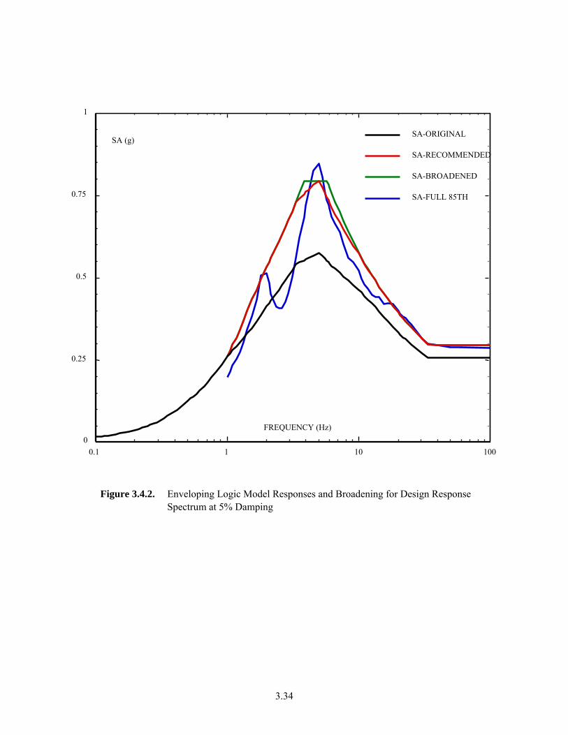
3.34
Figure 3.4.2. Enveloping Logic Model Responses and Broadening for Design Response Spectrum at 5% Damping
0
0.25
0.5
0.75
1
SA (g)
0.1 1 10 100
FREQUENCY (Hz)
FIGURE 1RECOMMENDED BROADED DRS
File: TREEOUT-R2-SPECTRA1.CRD
SA-FULL 85TH
SA-BROADENED
SA-RECOMMENDED
SA-ORIGINAL

3.35
Figure 3.4.3. Broadened Vertical Design Spectra at 5% Damping
0
0.1
0.2
0.3
0.4
0.5
SA (g)
0.1 1 10 100
FREQUENCY (Hz)
FIGUREVERTICAL BROADENED SPECTRA
File: VERTICAL-A.CRD
SV-BROADENED
SV-NEW
SV-OLD

3.36
Figure 3.4.4. Original 1996 and Revised 2005 Horizontal Design Spectra at 5% Damping
0
0.25
0.5
0.75
1
SA (g)
0.1 1 10 100
FREQUENCY (Hz)
SA-Revised 2005
SA-Original 1996
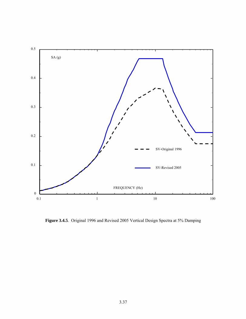
3.37
Figure 3.4.5. Original 1996 and Revised 2005 Vertical Design Spectra at 5% Damping
0
0.1
0.2
0.3
0.4
0.5
SA (g)
0.1 1 10 100
FREQUENCY (Hz)
SV-Revised 2005
SV-Original 1996

4.1
4.0 References
Abrahamson NA and WJ Silva. 1995. “A Consistent Set of Ground Motion Attenuation Relationships Including Data from the 19994 Northridge Earthquake.” Seismological Research Letters 66(2):23 (abstract). Abrahamson NA and WJ Silva. 1997. “Empirical Response Spectral Attenuation Relations for Shallow Crustal Earthquakes.” Seismological Research Letters 68(1):94-127. Anderson JG and SE Hough. 1984. “A Model for the Shape of the Fourier Amplitude Spectrum of Acceleration at High Frequencies.” Bulletin of the Seismological Society of America 74(5):1969-1993. Birdwell Division. 1979. Seismic Velocity Survey, Rockwell Hanford ESG, DC-2, -3, -4, -6, and -7, Benton County, Washington. Seismograph Service Corporation, Tulsa, Oklahoma. Boore DM. 1983. Stochastic Simulation of High-Frequency Ground Motions Based on Seismological Models of the Radiated Spectra.” Bulletin of the Seismological Society of America 73(6):1865-1894. Bozorgnia Y and KW Campbell. 2004. “The Vertical-to-horizontal Response Spectral Ratio and Tentative Procedures for Developing Simplified V/H and Vertical Design Spectra.” Journal of Earthquake Engineering 8(2):175-207. British Nuclear Fuels, Ltd. 1999. Validation of the Geomatrix Hanford Seismic Report for Use on the TWRS Privatization Project. RPT-W375-RU00004, Rev. 0, British Nuclear Fuels, Ltd., Richland, Washington. Campbell KW. 1994. “The Use of Attenuation Relationships Published by KW Campbell.” Memorandum to Walt Silva, Pacific Engineering and Analysis, Inc., August 15, 1994. Campbell KW and Y Bozorgnia. 2003. “Updated Near-Source Ground-Motion (Attenuation) Relations for the Horizontal and Vertical Components of Peak Ground Acceleration and Acceleration Response Spectra.” Bulletin of the Seismological Society of America 93(1):314-331. Electric Power Research Institute. 1993. Guidelines for Determining Design Basis Ground Motions. EPRI TR-102293, Volumes 1-5, Electric Power Research Institute, Palo Alto, California. Geomatrix Consultants, Inc. 1996. Probabilistic Seismic Hazard Analysis, DOE Hanford Site, Washington. WHC-SD-W236-TI-002, Rev. 1a, Westinghouse Hanford Company, Richland, Washington. Geomatrix Consultants, Inc. 2003. “Updated Relative Site Response Study for Hanford.” Calculation package prepared for Bechtel National, San Francisco, California.

4.2
Geovision Geophysical Services. 2004. DOE-ORP Waste Treatment Plant, Hanford, Washington, Test Well C-4652, Suspension P & S Velocities. Report 4398-01 prepared for Pacific Northwest National Laboratory, Richland, Washington. Holosonics, Inc. 1978. Seismic Logging Report, Holes DC-7 and DC-8, Hanford Works Reservation. Report to Fenix and Scisson, Inc., Richland, Washington. Northland Geophysical PLLC. 2004. Results of Downhole Seismic Velocity Surveys, Department of Energy Office of River Protection Waste Treatment Plant, Hanford Washington. Prepared for Pacific Northwest National Laboratory, Richland, Washington. Press WH, BP Flannery, SA Teukolsky, and WT Vetterling. 1986. Numerical Recipes. Cambridge University Press, Cambridge, United Kingdom. Reidel SP and DG Horton. 1999. Geologic Data Package for 2001, Immobilized Low-Activity Waste Performance Assessment. PNNL-12257, Rev. 1, Pacific Northwest National Laboratory, Richland, Washington. Robbins SL, JR Kunk, and FG Clutsom. 1983. Principal Facts and Density Estimates for Borehole Gravity Stations in Boreholes RRL-3, RRL-4, RRL-5, RRL-6B, RRL-7, RRL-8, and RRL-9 at the Hanford Site, Benton County, Washington. Open-File Report 83-386, U.S. Geological Survey; also RHO-BW-CR-139, Rockwell Hanford Operations, Richland, Washington. Robbins SL, RJ Martinez, and DL Smith. 1979. Principal Facts and Density Estimates for Borehole Gravity Stations in Wells DC-3, DC-5, DC-7 at the Hanford Site, Washington, and in Well RSH #1 on Rattlesnake Hills, Washington. Open File Report 79-849, U.S. Geological Survey. Rollins KM, MD Evans, NB Diehl, and WD Daily III. 1998. “Shear Modulus and Damping Relationships for Gravels.” Journal of Geotechnical and Geoenvironmental Engineering 124(5). Shannon & Wilson, Inc. 2000. Final Report, Geotechnical Investigation, River Protection Project-Waste Treatment Plant. Project No. DE-AC06-96RL-13308, Subcontract No. W375-WTSC99-1036, 200 East Area, Hanford Site, Richland, Washington, report prepared for British Nuclear Fuels, Ltd. Silva W. 1986. Soil Response to Earthquake Ground Motion. Research Project RP2556-07, report prepared for Electric Power Research Institute, Palo Alto, California. Silva, W. 1997. “Characteristics of vertical strong ground motions for applications to engineering design.” In Proceedings of the FHWA/NCEER Workshop on the National Representation of Seismic Ground Motion for New and Existing Highway Facilities. Technical Report NCEER-97-0010, National Center for Earthquake Engineering Research, Buffalo, New York.

4.3
Silva WC, N Abrahamson, G Toro, and C Costantino. 1998. Description and Validation of the Stochastic Ground Motion Model. Report submitted to Brookhaven National Laboratory, Associated Universities, Inc., Long Island, New York. Stokoe KH II, B Cox, Y-C Lin, MJ Jung, and A Kurtulus. 2005. Shear Wave Profiling at the Waste Treatment Plant Site, Hanford, WA. Geotechnical Engineering Report GR05-1, Geotechnical Engineering Center, University of Texas at Austin. Prepared for Pacific Northwest National Laboratory, Richland, Washington. U.S. Department of Energy. 1994. Natural Phenomena Hazards Design and Evaluation Criteria for Department of Energy Facilities. DOE-STD-1020-94, U.S. Department of Energy, Washington, D.C.

Appendix
Recommended Horizontal and Vertical Design Spectra for the Waste Treatment Plant

A.1
Appendix
Recommended Horizontal and Vertical Design Spectra for the Waste Treatment Plant
Table A.1. Recommended Horizontal and Vertical Design Spectra for the Waste Treatment Plant
FREQUENCY (HZ)
SA-HOR 1996 (g)
SA-HOR 2005 (g)
SV-VERT 1996 (g)
SV-VERT 2005 (g)
100.000 0.2570 0.2930 0.1750 0.2135 58.824 0.2570 0.2937 0.1750 0.2140 50.000 0.2570 0.2940 0.1750 0.2142 40.000 0.2570 0.2943 0.1980 0.2420 33.333 0.2570 0.2967 0.2190 0.2692 30.303 0.2698 0.3129 0.2309 0.2850 25.000 0.2975 0.3480 0.2567 0.3193 23.810 0.3050 0.3576 0.2638 0.3288 22.727 0.3123 0.3670 0.2706 0.3380 21.739 0.3194 0.3761 0.2773 0.3470 20.833 0.3264 0.3852 0.2839 0.3560 20.000 0.3333 0.3937 0.2904 0.3644 18.182 0.3498 0.4143 0.3061 0.3849 16.667 0.3657 0.4342 0.3212 0.4048 15.385 0.3809 0.4533 0.3358 0.4239 14.286 0.3955 0.4727 0.3498 0.4433 13.333 0.4097 0.4916 0.3634 0.4680 12.500 0.4213 0.5085 0.3640 0.4680 11.765 0.4326 0.5265 0.3646 0.4680 11.111 0.4435 0.5441 0.3651 0.4680 10.526 0.4541 0.5612 0.3657 0.4680 10.000 0.4644 0.5780 0.3662 0.4680 9.091 0.4783 0.6105 0.3610 0.4680 8.333 0.4913 0.6418 0.3563 0.4680 7.692 0.5037 0.6719 0.3521 0.4680 7.143 0.5153 0.7011 0.3481 0.4680 6.667 0.5264 0.7294 0.3446 0.4680 6.250 0.5371 0.7570 0.3413 0.4680 6.000 0.5439 0.7749 0.3392 0.4680 5.882 0.5472 0.7838 0.3381 0.4680 5.750 0.5511 0.7941 0.3370 0.4680

A.2
Table A.1. (continued)
FREQUENCY (HZ)
SA-HOR 1996 (g)
SA-HOR 2005 (g)
SV-VERT 1996 (g)
SV-VERT 2005 (g)
5.556 0.5570 0.7941 0.3353 0.4680 5.263 0.5664 0.7941 0.3326 0.4680 5.000 0.5754 0.7941 0.3300 0.4593 4.545 0.5673 0.7941 0.3212 0.4436 4.167 0.5599 0.7941 0.3133 0.4297 4.000 0.5565 0.7941 0.3097 0.4233 3.846 0.5532 0.7941 0.3062 0.4173 3.571 0.5471 0.7594 0.2998 0.4061 3.333 0.5415 0.7294 0.2940 0.3960 3.125 0.5231 0.7011 0.2838 0.3804 2.941 0.5064 0.6756 0.2746 0.3664 2.778 0.4912 0.6524 0.2662 0.3536 2.632 0.4771 0.6310 0.2585 0.3419 2.500 0.4642 0.6115 0.2514 0.3311 2.381 0.4523 0.5935 0.2448 0.3212 2.273 0.4411 0.5768 0.2386 0.3121 2.174 0.4308 0.5613 0.2330 0.3036 2.083 0.4211 0.5469 0.2276 0.2957 2.000 0.4120 0.5334 0.2226 0.2882 1.818 0.3868 0.4970 0.2076 0.2667 1.667 0.3651 0.4644 0.1947 0.2476 1.538 0.3463 0.4363 0.1835 0.2312 1.429 0.3297 0.3993 0.1738 0.2105 1.333 0.3150 0.3676 0.1652 0.1928 1.250 0.3018 0.3402 0.1575 0.1775 1.176 0.2899 0.3163 0.1506 0.1643 1.111 0.2792 0.2954 0.1444 0.1528 1.053 0.2693 0.2769 0.1388 0.1427 1.000 0.2603 0.2603 0.1336 0.1336 0.909 0.2351 0.2351 0.1235 0.1235 0.833 0.2141 0.2141 0.1149 0.1149 0.769 0.1965 0.1965 0.1075 0.1075 0.714 0.1815 0.1815 0.1011 0.1011 0.667 0.1686 0.1686 0.0955 0.0955 0.625 0.1573 0.1573 0.0906 0.0906 0.588 0.1474 0.1474 0.0861 0.0861 0.556 0.1387 0.1387 0.0822 0.0822 0.526 0.1309 0.1309 0.0786 0.0786 0.500 0.1239 0.1239 0.0753 0.0753 0.455 0.1088 0.1088 0.0676 0.0676 0.417 0.0967 0.0967 0.0613 0.0613 0.385 0.0867 0.0867 0.0560 0.0560

A.3
Table A.1. (continued)
FREQUENCY
(HZ)
SA-HOR 1996 (g)
SA-HOR 2005 (g)
SV-VERT 1996 (g)
SV-VERT 2005 (g)
0.357 0.0784 0.0784 0.0515 0.0515 0.333 0.0714 0.0714 0.0476 0.0476 0.313 0.0654 0.0654 0.0443 0.0443 0.294 0.0603 0.0603 0.0414 0.0414 0.278 0.0557 0.0557 0.0387 0.0387 0.263 0.0518 0.0518 0.0365 0.0365 0.250 0.0483 0.0483 0.0344 0.0344 0.238 0.0452 0.0452 0.0326 0.0326 0.227 0.0424 0.0424 0.0309 0.0309 0.217 0.0400 0.0400 0.0295 0.0295 0.208 0.0377 0.0377 0.0280 0.0280 0.200 0.0357 0.0357 0.0268 0.0268 0.182 0.0313 0.0313 0.0240 0.0240 0.167 0.0279 0.0279 0.0218 0.0218 0.154 0.0250 0.0250 0.0199 0.0199 0.143 0.0226 0.0226 0.0183 0.0183 0.133 0.0206 0.0206 0.0170 0.0170 0.125 0.0188 0.0188 0.0157 0.0157 0.118 0.0174 0.0174 0.0147 0.0147 0.111 0.0161 0.0161 0.0138 0.0138 0.100 0.0139 0.0139 0.0122 0.0122