Heriot-Watt University Research Gateway

Heriot-Watt University

Six-dimensional superconformal field theories from principal 3-bundles over twistor spaceSaemann, Christian; Wolf, Martin

Published in:Letters in Mathematical Physics

DOI:10.1007/s11005-014-0704-3

Publication date:2014

Document VersionPeer reviewed version

Link to publication in Heriot-Watt University Research Portal

Citation for published version (APA):Saemann, C., & Wolf, M. (2014). Six-dimensional superconformal field theories from principal 3-bundles overtwistor space. Letters in Mathematical Physics, 104(9), 1147-1188. DOI: 10.1007/s11005-014-0704-3

General rightsCopyright and moral rights for the publications made accessible in the public portal are retained by the authors and/or other copyright ownersand it is a condition of accessing publications that users recognise and abide by the legal requirements associated with these rights.

If you believe that this document breaches copyright please contact us providing details, and we will remove access to the work immediatelyand investigate your claim.

EMPG–13–07

DMUS–MP–13/12

Six-Dimensional Superconformal Field Theories

from Principal 3-Bundles over Twistor Space

Christian Samanna and Martin Wolf b ∗

a Maxwell Institute for Mathematical Sciences

Department of Mathematics, Heriot–Watt University

Edinburgh EH14 4AS, United Kingdom

b Department of Mathematics, University of Surrey

Guildford GU2 7XH, United Kingdom

Abstract

We construct manifestly superconformal field theories in six dimensions which

contain a non-Abelian tensor multiplet. In particular, we show how principal

3-bundles over a suitable twistor space encode solutions to these self-dual tensor

field theories via a Penrose–Ward transform. The resulting higher or categori-

fied gauge theories significantly generalise those obtained previously from prin-

cipal 2-bundles in that the so-called Peiffer identity is relaxed in a systematic

fashion. This transform also exposes various unexplored structures of higher

gauge theories modelled on principal 3-bundles such as the relevant gauge trans-

formations. We thus arrive at the non-Abelian differential cohomology that

describes principal 3-bundles with connective structure.

28th April 2014

∗E-mail addresses: c.saemann@hw.ac.uk, m.wolf@surrey.ac.uk

Contents

1 Introduction . . . . . . . . . . . . . . . . . . . . . . . . . . . . . . . . . . . . . . 1

2 Gauge structure: Lie 3-groups and Lie 2-crossed modules . . . . . . . . . . . . . 4

2.1 Lie crossed modules and differential crossed modules . . . . . . . . . . . . 4

2.2 Lie 2-crossed modules and differential 2-crossed modules . . . . . . . . . . 5

3 Principal 3-bundles . . . . . . . . . . . . . . . . . . . . . . . . . . . . . . . . . . 8

3.1 Cocycle description of principal 1- and 2-bundles . . . . . . . . . . . . . . 8

3.2 Cocycle description of principal 3-bundles . . . . . . . . . . . . . . . . . . 10

4 Penrose–Ward transform and self-dual fields . . . . . . . . . . . . . . . . . . . . 12

4.1 Outline of the Penrose–Ward transform . . . . . . . . . . . . . . . . . . . . 13

4.2 Twistor space . . . . . . . . . . . . . . . . . . . . . . . . . . . . . . . . . . 14

4.3 Penrose–Ward transform . . . . . . . . . . . . . . . . . . . . . . . . . . . . 15

4.4 Discussion of the constraint equations . . . . . . . . . . . . . . . . . . . . 29

4.5 Constraint equations and superconformal field equations . . . . . . . . . . 31

5 Higher gauge theory on principal 3-bundles . . . . . . . . . . . . . . . . . . . . . 33

6 Conclusions . . . . . . . . . . . . . . . . . . . . . . . . . . . . . . . . . . . . . . 37

Appendix . . . . . . . . . . . . . . . . . . . . . . . . . . . . . . . . . . . . . . . . . . 39

A Collection of Lie 2-crossed module identities and their proofs . . . . . . . . 39

1. Introduction

Following the impressive success of M2-brane models in the last few years, there is more

and more interest in six-dimensional superconformal field theories that might yield can-

didate theories for similar M5-brane models. These theories should exhibit N = (2, 0)

supersymmetry and have a tensor multiplet in their field content. The biggest issue in

the construction of such theories is to render the tensor fields non-Abelian in a meaningful

way. While there are a few ad-hoc prescriptions of how to do this, the geometrically most

appealing solution to this problem at the moment seems to be higher gauge theory, see

e.g. Baez & Huerta [1] and references therein.

Higher gauge theory describes consistently the parallel transport of extended objects,

just as ordinary gauge theory describes the parallel transport of point-like objects. This de-

scription arises from a categorification of the ingredients of ordinary gauge theory. Roughly

speaking, under categorification a mathematical notion is replaced by a category in which

the notion’s original structure equations hold only up to isomorphisms. When categorifying

principal bundles, we replace the gauge or structure groups by so-called Lie 2-groups (cer-

tain monoidal tensor categories) and the principal bundles by so-called principal 2-bundles

(a non-Abelian generalisation of gerbes).

1

Once a gauge structure is encoded in a way that allows for a description in terms of

Cech cochains (as e.g. principal bundles or bundle gerbes), we can construct a corres-

ponding field theory using twistor geometric techniques: the twistor space P 6 suitable for

discussing six-dimensional chiral field theories is well known. It is the space that paramet-

rises totally null 3-planes in six-dimensional space-time [2]. In addition, a generalisation

of the Penrose–Ward transform will map the Cech cochains to certain differential forms

encoding a categorified connection on six-dimensional space-time that satisfies a set of field

equations.

The Penrose–Ward transform for Abelian gerbes over P 6 was discussed in [3, 4] (see

also [5] for an earlier account and [6] for a supersymmetric extension). It yields u(1)-valued

self-dual 3-forms in six dimensions. Besides that, in [3,4,6] also twistor space actions have

been formulated that represent the twistor analogue of the space-time actions of Pasti,

Sorokin & Tonin [7].

More recently, we have presented the extension to the non-Abelian case [8]: certain

non-Abelian gerbes (or principal 2-bundles) over P 6 are mapped under a Penrose–Ward

transform to the connective structure of a non-Abelian gerbe on space-time that comes with

a self-dual 3-form curvature. Since the twistor space P 6 can be straightforwardly extended

to the supersymmetric case, a Penrose–Ward transform can also be used to identify non-

Abelian N = (2, 0) and N = (1, 0) superconformal field equations containing a tensor

multiplet and to describe solutions to these [8].

The principal 2-bundles that are available in the mathematical literature and that

have been developed to the extent necessary for applying our Penrose–Ward transform are

relatively restricted. Instead of having a fully categorified Lie group (a so-called weak Lie

2-group) as a gauge group, they only come with what is known as a strict Lie 2-group.

The latter can be regarded as a Lie crossed module, that is, a 2-term complex H → G of

ordinary Lie groups G and H. The 3-form curvature of a principal 2-bundle has to satisfy

a condition for the underlying parallel transport along surfaces to be well-defined. For a

principal 2-bundles with strict Lie 2-structure group, this implies that the 3-form curvature

takes values in the centre of the Lie algebra of H.

This restriction may be regarded as one of the drawbacks of this type of non-Abelian

gerbes, and from a topological perspective, these principal 2-bundles thus appear less

interesting. We would like to stress, however, that we expect principal 2-bundles still

to be relevant from a physical perspective. For instance, the field equations obtained

in [8] represent an interacting, non-Abelian set of tensor field equations. Moreover, in [9]

the 3-Lie algebra valued tensor field equations of Lambert & Papageorgakis [10] have

been recast in a higher gauge theory form based on principal 2-bundles. These equations

2

have been studied in detail (see e.g. [11] and references therein), and clearly contain non-

trivial dynamics. In particular, after a dimensional reduction, one recovers five-dimensional

maximally supersymmetric Yang–Mills theory.

We can avoid the aforementioned drawback in essentially two ways that remain man-

ageable with the tools available in the literature: first of all, one can work with infinite-

dimensional (Lie) crossed modules such as models of the string 2-group discussed by Baez

et al. [12]. This approach has been followed by a number of people, see for example

Fiorenza, Sati & Schreiber [13]. Note that because our twistor constructions [8] do not

make use of any explicit properties of finite-dimensional crossed modules, they extend

to such infinite-dimensional crossed modules without alteration. In the second approach,

one can categorify one step further and employ so-called principal 3-bundles having Lie

3-groups as structure 3-groups. Here, the 3-form curvature can take values in more general

subalgebras which are non-Abelian, in general. For a more detailed discussion of this point

in a more general context, see also [14]. In this paper, we shall develop the latter approach.

Principal 3-bundles come with 1-form, 2-form and 3-form gauge potentials together

with 2-form, 3-form and 4-form curvatures satisfying certain compatibility relations. If we

draw our motivation for the development of superconformal field theories in six dimensions

from M-theory with its 3-form potential, the inclusion of such a 3-from potential in the field

theory is rather natural. Further motivation for using principal 3-bundles stems from the

recently developed N = (1, 0) superconformal models [15–20], which make use of a 3-form

gauge potential.1 For other recent approaches to defining six-dimensional superconformal

theories, see e.g. references [10,21,13].

Higher gauge theory on principal 3-bundles has been developed to a certain extent,

see for example Martins & Picken [22], but various details still remain to be clarified.

We therefore have two goals in this paper: firstly, we will derive the equations of motion

of six-dimensional superconformal models with manifest N = (n, 0) supersymmetry for

n = 0, 1, 2 and encode their solutions in terms of holomorphic principal 3-bundles on twistor

space. In deriving the solutions from this holomorphic data, many properties of higher

gauge theory on principal 3-bundles (as e.g. the explicit form of finite and infinitesimal

gauge transformations) will become evident. Describing these properties together with the

differential cohomology underlying principal 3-bundles with connection is then our second

goal.

This paper is structured as follows. In Section 2, we start by reviewing the categorified

groups replacing ordinary gauge groups in our theories. We then present the cocycle de-

1Note, however, that it seems clear that these models do not directly fit the picture of higher gauge theory

on principal 3-bundles, at least not without extending the gauge Lie 3-algebra to a 3-term L∞-algebra.

3

scription of principal 3-bundles in Section 3, which we will use in a rather involved Penrose–

Ward transform in Section 4. In Section 4.4, we discuss the resulting six-dimensional su-

perconformal field theories in detail. In Section 5, we summarise what we have learnt about

principal 3-bundles with connective structure by formulating the underlying non-Abelian

differential cohomology. We conclude in Section 6.

2. Gauge structure: Lie 3-groups and Lie 2-crossed modules

The definition of parallel transport of objects that are not point-like and transform under

non-Abelian groups has been a long-standing problem. This problem is closely related

to that of defining non-Abelian Cech (and Deligne) cohomology beyond the cohomology

set encoding vector bundles. A way to solving both problems is by categorifying the usual

description of gauge theory in terms of principal bundles as explained, for instance, in Baez

& Huerta [1]. In particular, we will have to categorify the notion of a structure group of a

principal bundle.

As already indicated, the general categorifications of the notion of a Lie group lead

to so-called weak Lie n-groups. To our knowledge, the theory of principal n-bundles with

weak Lie n-groups as structure n-groups has not been developed, at least not to the degree

that our constructions require. We therefore have to restrict ourselves to semistrict Lie 3-

groups that are encoded by a Lie 2-crossed module, just as strict Lie 2-groups are encoded

by Lie crossed modules. Both Lie crossed modules and Lie 2-crossed modules are very

manageable, as they consist of 2-term and 3-term complexes of Lie groups, respectively.

2.1. Lie crossed modules and differential crossed modules

In this section, we would like to review briefly the definitions of Lie crossed modules and

their infinitesimal version. For more details, see Baez & Lauda [23] and references therein.

Lie crossed modules. Let (G,H) be a pair of Lie groups. We call the pair (G,H) a Lie

crossed module if, in addition, there is a smooth G-action B on H by automorphisms2 (and

another one on G by conjugation) and a Lie group homomorphism t : H→ G such that the

following two axioms are satisfied:

2That is, g B (h1h2) = (g B h1)(g B h2) for all g ∈ G and h1, h2 ∈ H and furthermore, g1g2 B h = g1 B(g2 B h) for all g1, g2 ∈ G and h ∈ H.

4

(i) The Lie group homomorphism t : H → G is a G-homomorphism, that is,

t(g B h) = gt(h)g−1 for all g ∈ G and h ∈ H.

(ii) The G-action B and the Lie group homomorphism t : H→ G obey the so-called

Peiffer identity, t(h1) B h2 = h1h2h−11 for all h1, h2 ∈ H.

In the following, we shall write (Ht→ G,B) or simply H → G to denote a Lie crossed

module. Note that Lie crossed modules are in one-to-one correspondence with so-called

strict Lie 2-groups [23].

A simple example of a Lie crossed module is (Nt→ G,B), where N is a normal Lie

subgroup of the Lie group G, t is the inclusion, and B is conjugation. Another example

appears in the non-Abelian gerbes of Breen & Messing [24] for which the Lie crossed

module is the automorphism Lie 2-group (Gt→ Aut(G),B) of a Lie group G, where t is the

embedding via conjugation and B the identity.

Differential Lie crossed modules. The infinitesimal counterpart of a Lie crossed mod-

ule is a differential Lie crossed module. In particular, if (g, h) is a pair of Lie algebras

together with a g-action B on h by derivations3 (and on g by the adjoint representation)

and a Lie algebra homomorphism t : h → g, then we call (ht→ g,B) a differential Lie

crossed module provided the linearisations of the two axioms of a Lie crossed module are

satisfied:

(i) The Lie algebra homomorphism t : H→ G is a g-homomorphism, t(X B Y ) =

[X, t(Y )] for all X ∈ g and Y ∈ h, where [·, ·] denotes the Lie bracket on g.

(ii) The g-action B and the Lie algebra homomorphism t : h→ g obey the Peiffer

identity, t(Y1) B Y2 = [Y1, Y2] for all Y1,2 ∈ h, where [·, ·] denotes the Lie

bracket on h.

We shall again use h → g as a shorthand notation to denote a differential Lie crossed

module. In categorical language, differential Lie crossed modules are in one-to-one corres-

pondence with strict Lie 2-algebras. We would like to point out that, as shown in [9], the

3-algebras underlying the recently popular M2-brane models can be naturally described in

terms of differential Lie crossed modules.

2.2. Lie 2-crossed modules and differential 2-crossed modules

As indicated, Lie crossed modules (Ht→ G,B) are used as structure 2-groups in the theory

of principal 2-bundles, in the same way that Lie groups are the structure groups for principal

3That is, if we denote by [·, ·] the Lie brackets on g and h, respectively, then X B [Y1, Y2] = [X BY1, Y2] + [Y1, X B Y2] for all X ∈ g and all Y1,2 ∈ h and furthermore, [X1, X2] B Y = X1 B (X2 BY )−X2 B (X1 B Y ) for all X1,2 ∈ g and Y ∈ h.

5

bundles (that is, principal 1-bundles). The connective structure on a principal 2-bundle,

encoded in a g-valued connection 1-form and a h-valued connection 2-form, is, however,

somewhat restricted: its associated 3-form curvature has to take values in the kernel of t

for a consistent parallel transport. Together with the Peiffer identity, this implies that the

3-form curvatures lies in the centre of h.

We now wish to remove this undesirable restriction by moving away from Lie crossed

modules and turning to a categorification of them, the so-called Lie 2-crossed modules

of Conduche [25] together with their differential counterparts.4 As we shall see later,

these will be used as structure 3-groups in the theory of principal 3-bundles. Our main

motivation to consider this specific generalisation is that the Peiffer identity can be relaxed

in a systematic way by means of the so-called Peiffer lifting. As a direct consequence, the

condition that the 3-form curvature takes values in the centre of some Lie algebra will be

relaxed, too. This will eventually enable us to construct superconformal self-dual tensor

theories in six dimensions with a general 3-form curvature.

Lie 2-crossed modules. Let (G,H, L) be a triple of Lie groups. A Lie 2-crossed mod-

ule [25] is a normal complex5 of Lie groups,

Lt−→ H

t−→ G , (2.1)

together with smooth G-actions on H and L by automorphisms (and on G by conjugation),

both denoted by B, and a G-equivariant smooth mapping from H × H to L called the

Peiffer lifting and denoted by ·, · : H× H→ L,6 subject to the following six axioms (see

e.g. [25, 22]):

(i) The Lie group homomorphisms t are G-homomorphisms, that is, t(g B `) =

g B t(`) and t(g B h) = gt(h)g−1 for all g ∈ G, h ∈ H, and ` ∈ L.

(ii) t(h1, h2) = h1h2h−11 (t(h1) B h−12 ) for all h1, h2 ∈ H. We define 〈h1, h2〉 :=

h1h2h−11 (t(h1) B h−12 ).

(iii) t(`1), t(`2) = `1`2`−11 `−12 for all `1, `2 ∈ L. We define [`1, `2] := `1`2`

−11 `−12

(and likewise for elements of G and H).

4Another categorification of Lie crossed modules is given by Lie crossed squares and Breen [26] has

constructed higher principal bundles using those as structure groups. These crossed squares can be reduced

to 2-crossed modules and from a categorical perspective, the latter are sufficiently general.5The mappings t are Lie group homomorphisms with t2(`) = 1 for all ` ∈ L, the images of the mappings

t are normal Lie subgroups, and im(t : L→ H) is normal in ker(t : H→ L). This is a necessary requirement

for defining cohomology groups via coset spaces.6G-equivariance of ·, · means that g B h1, h2 = g B h1, g B h2 for all g ∈ G and h1, h2 ∈ H.

6

(iv) h1h2, h3 = h1, h2h3h−12 (t(h1) B h2, h3) for all h1, h2, h3 ∈ H.

(v) h1, h2h3 = h1, h2h1, h3〈h1, h3〉−1, t(h1) B h2 for all h1, h2, h3 ∈ H.

(vi) t(`), hh, t(`) = `(t(h) B `−1) for all h ∈ H and ` ∈ L.

We shall write (Lt→ H

t→ G,B, ·, ·) or, as shorthand notation, L → H → G to denote

a Lie 2-crossed module. From a categorical point of view, Lie 2-crossed modules encode

semistrict Lie 3-groups called Gray groups, see Kamps & Porter [27], i.e. Gray groupoids

with a single object.

Furthermore, there is an additional, natural H-action on L, also denoted by B, that is

induced by the above structure,

h B ` := `t(`)−1, h for all h ∈ H and ` ∈ L . (2.2)

This action is an H-action on L by automorphisms [25, 28], and we recall the proof in

Appendix A. We directly conclude that

g B (h B `) = (g B h) B (g B `) for all g ∈ G , h ∈ H , and ` ∈ L . (2.3)

We would like to emphasise that Lie crossed modules are special instances of Lie 2-

crossed modules, and, as such, the latter form natural generalisations of the former. This

can be seen as follows. Firstly, let us consider the situation when L is the trivial group

L = 1. Then, the data (Ht→ G,B) form a Lie crossed module since h1, h2 = 1 for all

h1, h2 ∈ H and the above axioms (i)–(vi) straightforwardly reduce to those of a Lie crossed

module. Secondly, for any Lie 2-crossed module (Lt→ H

t→ G,B, ·, ·), the truncation

(Lt→ H,B) with the induced H-action (2.2) forms a Lie crossed module, since from (2.2)

and axioms (ii) and (iii) it immediately follows that

t(h B `) = t(`)t(t(`−1), h) = t(`)t(`−1)ht(`)h−1 = ht(`)h−1 ,

t(`1) B `2 = `2t(`−12 ), t(`1) = `1`2`−11 .

(2.4)

These are precisely the two axioms of a Lie crossed module. Finally, the data (t(L)\H t→G,B) also forms a Lie crossed module.

Differential Lie 2-crossed modules. As before, we may study the infinitesimal coun-

terpart of Lie 2-crossed modules. Let (g, h, l) be a triple of Lie algebras. A differential Lie

2-crossed module is a normal complex of Lie algebras

lt−→ h

t−→ g , (2.5)

equipped with g-actions on h and l by derivations (and on g by the adjoint representation),

again denoted by B, respectively, and a g-equivariant bilinear map, called again Peiffer

7

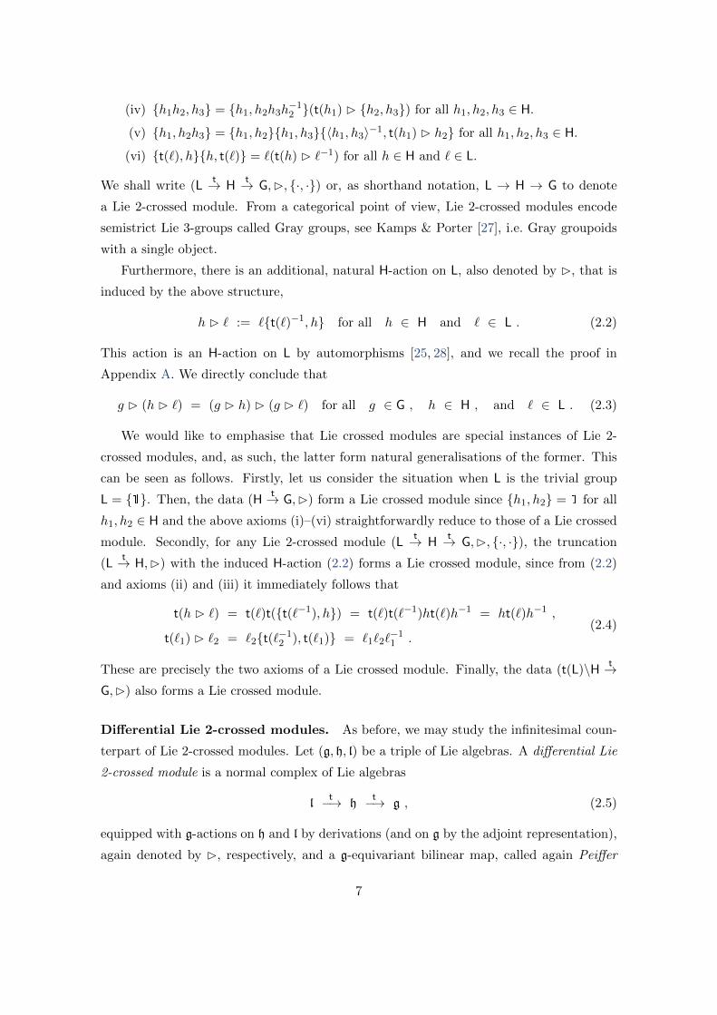
lifting and denoted by ·, · : h× h→ l, all of which satisfy the following axioms (here, [·, ·]denotes the Lie bracket in the respective Lie algebra):

(i) The Lie algebra homomorphisms t are g-homomorphisms, that is, t(X B Z) =

X B t(Z) and t(X B Y ) = [X, t(Y )] for all X ∈ g, Y ∈ h, and Z ∈ l.

(ii) t(Y1, Y2) = [Y1, Y2]− t(Y1) B Y2 =: 〈Y1, Y2〉 for all Y1,2 ∈ h.

(iii) t(Z1), t(Z2) = [Z1, Z2] for all Z1,2 ∈ l.

(iv) [Y1, Y2], Y3 = t(Y1) B Y2, Y3 + Y1, [Y2, Y3] − t(Y2) B Y1, Y3 −Y2, [Y1, Y3] for all Y1,2,3 ∈ h.

(v) Y1, [Y2, Y3] = t(Y1, Y2), Y3 − t(Y1, Y3), Y2 for all Y1,2,3 ∈ h.

(vi) t(Z), Y + Y, t(Z) = −t(Y ) B Z for all Y ∈ h and Z ∈ l.

We shall write (lt→ h

t→ g,B, ·, ·) or, more succinctly, l→ h→ g to denote a differential

Lie 2-crossed module.

Analogously to Lie 2-crossed modules, there is an induced h-action B on l that is defined

as

Y B Z := −t(Z), Y for all Y ∈ h and Z ∈ l (2.6)

and acts by derivations. This h-action simply follows from the linearisation of (2.2). In

addition, as is a direct consequence of the finite case, (lt→ h,B) forms a differential Lie

crossed module.

3. Principal 3-bundles

The next step in our discussion is the introduction of categorified principal bundles that are

modelled on Lie 2-crossed modules. Such bundles are called principal 3-bundles. Following

the conventional nomenclature of ordinary principal (1-)bundles, we shall refer to the Lie

2-crossed modules on which the principal 3-bundles are based as the structure 3-groups.

Notice that principal 1-bundles and 2-bundles as well as Abelian 1-gerbes and 2-gerbes will

turn out to be special instances of principal 3-bundles.

3.1. Cocycle description of principal 1- and 2-bundles

Firstly, let us briefly recall the formulation of smooth principal 1- and 2-bundles in terms

of Cech cohomology. To this end, let M be a smooth manifold and let Ua be a covering

of M which is chosen to be sufficiently fine. In the following, the intersections of coordinate

patches that appear will always be assumed to be non-empty.

8

Principal bundles. As is well-known, smooth principal bundles over M with structure

group G are described in terms of the non-Abelian Cech cohomology H1(M,G).7 Repres-

entatives of elements of H1(M,G) are 1-cocyles and are called transition functions. Spe-

cifically, a 1-cocycle is a collection gab of smooth maps gab : Ua ∩ Ub → G on non-empty

intersections Ua ∩ Ub which obey the cocycle condition

gabgbc = gac on Ua ∩ Ub ∩ Uc . (3.1)

Note that this condition implies that gaa = 1. Moreover, two principal bundles with trans-

ition functions gab and gab are considered topologically equivalent (or cohomologous),

if there are smooth maps ga : Ua → G such that

gab = g−1a gabgb . (3.2)

A trivial principal bundle is a principal bundle that is described by transition functions

that are all cohomologous to one, that is, gab ∼ 1 on all Ua ∩ Ub.

Principal 2-bundles. Similarly, smooth principal 2-bundles with structure 2-groups

(Ht→ G,B) can be described in terms of a generalised, non-Abelian Cech cohomology de-

noted by H2(M,H→ G). Representatives of elements of this cohomology set are 2-cocyles

and are again called transition functions. Specifically, a 2-cocycle is a pair (gab, habc)of collections of smooth maps gab : Ua ∩ Ub → G and habc : Ua ∩ Ub ∩ Uc → H which obey

the following cocycle conditions [24,29] (see also [30]):

t(habc)gabgbc = gac on Ua ∩ Ub ∩ Uc ,

hacdhabc = habd(gab B hbcd) on Ua ∩ Ub ∩ Uc ∩ Ud .(3.3)

The first equation is a ‘categorification’ of (3.1): the original equation holds only up to the

isomorphism t(habc). The second equation is the appropriate non-Abelian generalisation

of the defining relation of a Cech 2-cocycle.

Clearly, if H = 1, that is, H is the trivial group, then the definition (3.3) reduces to

that of an ordinary principal G-bundle. Moreover, for the Lie crossed module BU(1) :=

(U(1)t→ 1,B) with t and B trivial, this definition coincides with that of an Abelian

(bundle) gerbe. Finally, twisted principal bundles can also be regarded as certain principal

2-bundles. We would like to emphasise that, roughly speaking, the cohomology H2(M,H→G) combines ordinary first-order and second-order Cech cohomologies non-trivially: if both

7In writing H1(M,G), we do not make a notational distinction between the Lie group G and the sheaf

SG of smooth G-valued functions. We shall continue to use a similar notation when dealing with principal

2-bundles and 3-bundles, respectively.

9

H and G are Abelian and the action of G onto H is trivial, thenH2(M,H→ G) ∼= H1(M,G)⊕H2(M,H).

Two principal 2-bundles, represented by the transition functions (gab, habc) and

(gab, habc), are considered equivalent (or cohomologous), (gab, habc) ∼ (gab, habc),if there are smooth maps ga : Ua → G and hab : Ua ∩ Ub → H such that

gagab = t(hab)gabgb and hachabc = (ga B habc)hab(gab B hbc) . (3.4)

A trivial principal 2-bundle is then described by transition functions that are all cohomo-

logous to one, that is, gab ∼ 1 on all Ua ∩ Ub and habc ∼ 1 on all Ua ∩ Ub ∩ Uc.Note that by virtue of (3.4), we can always assume that haaa = 1 without loss of

generality. Concretely, starting from a general habc with haaa 6= 1, it is a straightforward

exercise to show that for the choice haa = haaa we obtain haaa = 1. In the following, we shall

therefore always make this choice and assume haaa = 1. Clearly, the residual equivalence

relations are then those relations (3.4) for which haa = 1. Furthermore, from (3.3) together

with haaa = 1 we immediately conclude that also gaa = 1 and haab = habb = 1.

3.2. Cocycle description of principal 3-bundles

General 3-cocyles. Let us now move on and discuss smooth principal 3-bundles. There

are two obvious ways of categorifying Lie crossed modules and therefore two routes to

principal 3-bundles. The first one, using ‘crossed modules of crossed modules’ also known

as crossed squares, yields the 2-gerbes of Breen [26, 31]. The second one, which we shall

be following here, was developed by Jurco in [32] and uses 2-crossed modules (Lt→ H

t→G,B, ·, ·). It leads to a nice categorification of the cocycle description (3.3) in terms

of a specific generalised, non-Abelian Cech cohomology, denoted by H3(M, L → H → G)

in the following. Representatives of elements of this non-Abelian cohomology set are 3-

cocycles which are collections (gab, habc, `abcd) of smooth maps gab : Ua ∩ Ub → G,

habc : Ua ∩Ub ∩Uc → H, and `abcd : Ua ∩Ub ∩Uc ∩Ud → L subject to the following cocycle

conditions [32]8:

t(habc)gabgbc = gac on Ua ∩ Ub ∩ Uc , (3.5a)

hacdhabct(`abcd) = habd(gab B hbcd) on Ua ∩ Ub ∩ Uc ∩ Ud , (3.5b)

and

`abcd((gab B h−1bcd) B `abde)(gab B `bcde) =

= (h−1abc B `acde)h−1abc, gac B h−1cde((gabgbc B h−1cde) B `abce) . (3.5c)

8The convention in comparison to [32] are as follows: nij ↔ gab, mijk ↔ h−1abc and `ijkl ↔ `abcd.

10

on Ua ∩ Ub ∩ Uc ∩ Ud ∩ Ue. The first equation is the same as that for a principal 2-bundle.

The next equation is a ‘categorification’ of the corresponding equation of a principal 2-

bundle. The last equation is the appropriate non-Abelian generalisation of the Abelian

Cech cocycle equation; see [32] for details on the derivation. As before, we will refer to the

3-cocycles as transition functions.

From the above equations it is clear that the cohomology H3(M, L → H → G) com-

bines ordinary first-order, second-order, and third-order Cech cohomologies in a non-trivial

fashion: if L, H, and G are all Abelian and the action of G onto H and L is trivial, then

H3(M, L → H → G) ∼= H1(M,G) ⊕ H2(M,H) ⊕ H3(M, L). Note that these principal

3-bundles are a non-Abelian generalisation of principal 2-bundles that contain Abelian 2-

gerbes: for L = 1, the cocycle conditions (3.5) reduce to the ones of a principal 2-bundle.

Moreover, for the Lie 2-crossed module BBU(1) = (U(1)t→ 1 t→ 1), we recover the

definition of a local Abelian (bundle) 2-gerbe. Note that twisted gerbes are special cases

of principal 3-bundles.

Two principal 3-bundles described by transition functions (gab, habc, `abcd) and

(gab, habc, ˜abcd) are considered equivalent, if there are smooth maps ga : Ua → G,

hab : Ua ∩ Ub → H and `abc : Ua ∩ Ub ∩ Uc → L such that

gagab = t(hab)gabgb , (3.6a)

hachabc = (ga B habc)hab(gab B hbc)t(`abc) , (3.6b)

`abcd = (h−1abc B `acd)(h−1abc B (gac B h−1cd )) B

B[`abc(((gab B hbc)hab) B ga B ˜

abcd)(h−1ab B hab, gb B h−1bc )

]×

× (h−1ab B hab, (h−1abc B gac B h−1cd )×

× ((t(h−1abc)gac) B h−1cd )(h−1abc B gac B h−1cd ))h−1abc, gac B h−1cd ×

× (gab B `−1bcd)(h−1ab B hab, gab B t(`bcd))×

× ((gab B h−1bcd)h−1ab B hab, gab B hbcd)×

× ((gab B h−1bcdh−1bd )h−1ab B hab, gab B hbd)((gab B h−1bcd) B `−1abd) . (3.6c)

Similarly to the principal 2-bundle case, these equivalence relations can be used to

normalise the transition functions according to

gaa = 1 , haab = habb = 1 , and `aabc = `abbc = `abcc = 1 , (3.7)

and we shall always do so in the following.

Trivial 3-cocyles. For a trivial principal 3-bundle, there exist smooth maps ga : Ua → G,

hab : Ua ∩ Ub → H, and `abc : Ua ∩ Ub ∩ Uc → L such that the transition functions satisfy

11

the following conditions:

gab = t(h−1ab )gag−1b , (3.8a)

habc = h−1ac hab(gab B hbc)t(`−1abc) , (3.8b)

`abcd = (h−1abc B `acd)h−1abc, gac B h−1cd ×

× ((gabgbc B h−1cd ) B `abc)(gab B `−1bcd)((gab B h−1bcd) B `−1abd) . (3.8c)

These relations can be derived from (3.6) by putting gab = 1, habc = 1, and ˜abc = 1.

Alternatively, the first of these equations can be read off (3.5a) by fixing the patch where

the cocycle trivialises to be Uc. Likewise, (3.8b) follows from (3.5b) by fixing the trivialising

patch to be Ud and (3.8c) follows from (3.5c) by fixing the trivialising patch to be Ue,

respectively. Note that to preserve the normalisations (3.7), we also normalise the group-

valued functions hab and `abc according to

haa = 1 and `aaa = `aab = `abb = 1 . (3.9)

Finding the splitting (3.8) for a given collection of transition functions (gab, habc, `abcd)amounts to solving a Riemann–Hilbert problem.

4. Penrose–Ward transform and self-dual fields

We are now in the position to pursue our main idea to construct self-dual non-Abelian

tensor field theories in six dimensions via twistor theory. The basic idea of twistor theory

is to encode solutions to certain field equations on space-time in terms of holomorphic data

on a twistor space that is associated with space-time in a particular fashion. Conversely,

the field equations in question and the associated gauge transformations follow naturally

from the algebraic twistor data. For gauge theory, this map between data on space-time

and data on twistor space is known as a Penrose–Ward transform.

The twistor approach has been used very successfully for the description of instantons

in Yang–Mills theory [33] and Einstein gravity [34] in four dimensions (including their

supersymmetric extensions, e.g. in [35–38]). In this context, the twistor space is the Penrose

twistor space [39] (and supersymmetric extensions thereof, see for example [40,35,37]) and

the holomorphic twistor data are certain holomorphic vector and principal bundles in

the case of Yang–Mills theory and holomorphic contact structures in the case of Einstein

gravity. The twistor approach has also been used for description of gauge theory instantons

in dimensions greater than four (see, e.g. [41] and references therein). In addition, it has

been used to describe equations of motion of non-self-dual theories such as maximally

supersymmetric Yang–Mills theory in four [42,35], three [43], and six dimensions [44].

12

More recently, it was demonstrated that twistor theory can also be applied to the

construction of superconformal non-Abelian self-dual tensor field theories in six dimensions

[8] which are based on principal 2-bundles (see [3–6] for the Abelian description). In the

remainder of this work, we would like to generalise our previous results [8] by constructing

superconformal self-dual non-Abelian tensor field theories in six dimensions that are based

on principal 3-bundles. As indicated previously, principal 3-bundles allow to relax the

Peiffer identity, and, as such, we will obtain self-dual tensor theories with a 3-form curvature

that is significantly less constrained than that of principal 2-bundles.

4.1. Outline of the Penrose–Ward transform

Since the following construction is rather lengthy and technical, let us give a brief overview

over the key components and present an outline of the Penrose–Ward transform discussed

in this section. We are interested in an N = (n, 0) superconformal gauge theory in six

dimensions, and we start by constructing a twistor space P 6|8n to six-dimensional flat

Minkowski superspace M6|8n. Relating both spaces is the so-called correspondence space

F 9|8n, which is fibred over both P 6|8n and M6|8n:

P 6|2n M6|8n

F 9|8n

π1 π2

@@R

(4.1)

The aim of the Penrose–Ward transform is now to establish a bijection between certain

topologically trivial holomorphic principal 3-bundles over twistor space P 6|2n and solutions

to the superconformal gauge theory over M6|8n. Starting from such a principal 3-bundle

E → P 6|2n, we pull it back along π1. The resulting principal 3-bundle E on correspond-

ence space F 9|8n turns out to be holomorphically trivial. There exists now a differential

cohomology relative to π1, which translates between a holomorphically trivial principal

3-bundle with non-trivial transition functions but vanishing relative connective structure

and a principal 3-bundle with trivial transition functions and flat but non-vanishing rel-

ative connective structure. The explicit construction of this equivalence relation will turn

out to be the most involved part of our construction. The resulting flat relative connective

structure on correspondence space can be readily pushed down to M6|8n. Relative flatness

translates into certain constraint equations which are fulfilled by the connective structure

on M6|8n. These constraint equations are equivalent to the field equations of the supercon-

formal field theory we are interested in. Besides the constraint equations, our construction

also exposes the full gauge symmetry of connective structures on principal 3-bundles.

13

4.2. Twistor space

Chiral superspace. As we wish to discuss superconformal gauge theories in six dimen-

sions, let us consider complexified flat space-time, M6 := C6, and extend it by 8n fermionic

directions with n ∈ 0, 1, 2. We obtain N = (n, 0) chiral superspace M6|8n := C6|8n :=

C6⊕ΠC8n, where Π is the (Graßmann) parity-changing operator. We will always work in

this complexified setting; real structures leading to Minkowski signature or split signature

can be introduced whenever desired (see, e.g., [3] for details).

Next, we coordinatise chiral superspace M6|8n by (xAB, ηAI ), where the xAB = −xBA

are bosonic (i.e. Graßmann-parity even) coordinates and the ηAI are fermionic (i.e. Graß-

mann-parity odd) coordinates. The indices A,B, . . . = 1, . . . , 4 are (anti-chiral) spinor

indices and I, J, . . . = 1, . . . , 2n are Sp(n) R-symmetry indices. Anti-symmetric pairs of

spinor indices may be raised and lowered with the help of the Levi-Civita symbol 12εABCD.

Specifically, we shall write xAB := 12εABCDx

CD.

If we let Ω := (ΩIJ) be an Sp(n)-invariant 2n × 2n matrix, we may introduce the

derivative operators

PAB :=∂

∂xAB:= ∂AB and DI

A :=∂

∂ηAI− 2ΩIJηBJ

∂

∂xAB. (4.2)

They obey the (anti-)commutation relations

[PAB, PCD] = 0 , [PAB, DIA] = 0 , and [DI

A, DJB] = −4ΩIJPAB , (4.3)

where [·, ·] denotes the super Lie bracket (graded supercommutator).

In the following, we will use the conventions ∂ABxCD = δ

[C[Aδ

D]B] , where brackets denote

normalised anti-symmetrisation of the enclosed indices.9

Twistor space and double fibration. To define the relevant twistor space of M6|8n,

we first introduce the correspondence space, which we define as F 9|8n := M6|8n ×P3 with

P3 being complex projective 3-space. Furthermore, we equip the correspondence space

with the coordinates (xAB, ηAI , λA), where the λA are homogeneous coordinates10 on P3.

Notice that for n = 0, the correspondence space can be understood as the projectivisation

of the dual of the (rank-4) bundle of anti-chiral spinors on six-dimensional space-time M6.

On F 9|8n, we introduce a distribution D := spanV A, V IAB, called the twistor distri-

bution, with

V A := λB∂AB and V IAB := 1

2εABCDλCD

ID . (4.4)

9Likewise, parentheses will denote normalised symmetrisation of the enclosed indices.10In particular, all equations involving these homogeneous coordinates are obviously to be understood as

homogeneous equations.

14

This is a rank-3|6n distribution because of the relations λAVA = 0 = λBV

IAB. Moreover, it

is a straightforward exercise to check that D is an integrable distribution, that is, [D,D] ⊆D. Therefore, we have a foliation of the correspondence space, and we define the twistor

space to be the quotient P 6|2n := F 9|8n/D. This is a complex (super)manifold. Indeed, if

we let (zA, λA, ηI) be homogeneous coordinates on P7|2n, then the twistor space P 6|2n is a

complex hypersurface in P7|2n \P3|2n given by the zero locus

zAλA − ΩIJηIηJ = 0 , (4.5)

where the P3|2n we remove from P7|2n is given by the condition λA = 0.

In summary, we have established the double fibration (4.1), where π2 denotes the trivial

projection while π1 acts as

π1 : (xAB, ηAI , λA) 7→ (zA, ηI , λA) = ((xAB + ΩIJηAI ηBJ )λB , ηAI λA , λA) . (4.6)

The equations

zA = (xAB + ΩIJηAI ηBJ )λB and ηI = ηAI λA (4.7)

are called the incidence relation.

Geometric twistor correspondence. Because of the incidence relation (4.7), we have

a geometric relation between points and certain submanifolds. Specifically, any point x ∈M6|8n in chiral superspace corresponds to a complex projective 3-space x = π1(π

−12 (x)) →

P 6|2n. Conversely, any point p ∈ P 6|2n in twistor space corresponds to a 3|6n-superplane

π2(π−11 (p)) →M6|8n,

xAB = xAB0 + εABCDµCλD + 2ΩIJεCDE[AλCθIDEη0B]J ,

ηAI = η0AI + εABCDλBθICD .

(4.8)

Here, (xAB0 , η0AI ) is a particular solution to the incidence relation (4.7) which corresponds

to a reference point in the superplane in M6|8n. The moduli µA and θIAB are defined up

to terms proportional to λA. As a result, there are 3|6n (which is the rank of the twistor

distribution) moduli parametrising the superplane. Note that for n = 0, (4.8) reduce to

xAB = xAB0 + εABCDµCλD and εABCDµCλD is a generic null-vector in six dimensions.

Hence, (4.8) represent a super-extension of a totally null 3-plane.

4.3. Penrose–Ward transform

Twistor data. Subject of this section is the explicit derivation of non-Abelian self-dual

tensor theories by means of twistor theory. In particular, the algebraic twistor data from

15

which we would like to start is represented by topologically trivial, holomorphic principal

3-bundles E → P 6|2n over the twistor space P 6|2n which, in addition, are holomorphically

trivial when restricted to any complex projective 3-space x = π1(π−12 (x)) → P 6|2n. Follow-

ing Manin’s terminology in the principal 1-bundle case [35], we will refer to such bundles

as M6|8n-trivial. We denote the structure 3-group of E by (Lt→ H

t→ G,B, ·, ·).11 If, as

before, Ua is an open covering of P 6|2n that is chosen to be sufficiently fine (Stein), then

E → P 6|2n can be described by holomorphic transition functions (gab, habc, ˆabcd)on appropriate non-empty overlaps of the coordinate patches Ua subject to the cocycle

conditions (3.5) and the normalisations (3.7).12

Relative connective structure. Next, we wish to pull back such an M6|8n-trivial

bundle E → P 6|2n to the correspondence space along the projection π1. This yields a

holomorphic principal 3-bundle E := π∗1E over F 9|8n. For simplicity, we work with the in-

duced covering Ua := π−11 (Ua) on the correspondence space. This enables us to describe

the bundle E in terms of the pulled-back transition functions (gab := π∗1 gab, habc :=

π∗1habc, `abcd := π∗1ˆabcd) which also obey (3.7). Since we are assuming that the bundle

E → P 6|2n is topologically trivial, and, in addition, holomorphically trivial on all pro-

jective 3-spaces x = π1(π−12 (x)), the bundle E → F 9|8n must be trivial (topologically as

well as holomorphically) on all of the correspondence space. Hence, by virtue of (3.8), its

transition functions are of the form

gab = t(h−1ab )gag−1b , (4.9a)

habc = h−1ac hab(gab B hbc)t(`−1abc) , (4.9b)

`abcd = (h−1abc B `acd)h−1abc, gac B h−1cd ×

× ((gabgbc B h−1cd ) B `abc)(gab B `−1bcd)((gab B h−1bcd) B `−1abd) . (4.9c)

We emphasise that the group-valued functions (ga, hab, `abc) are holomorphic and

obey (3.9). Despite being holomorphically trivial, the bundle E → F 9|8n contains non-

trivial information: the explicit equivalence relation turning the transition functions de-

scribing E to trivial ones generate a non-trivial relative connective structure as will become

transparent momentarily.

11At this stage, we could assume that L, H, and G are Lie supergroups, and hence, E is a principal

3-superbundle. However, for the sake of clarity, and since there is no immediate physical application of

supergroups here, we will only work with Lie groups. The discussion below can be adapted to the supergroup

case without any difficulty.12The standard (Stein) cover of P 6|2n consists of four coordinate patches. Hence, for this choice of cover,

there will only be one `abcd, and, consequently, the cocycle condition (3.5c) for `abcd will become vacuous.

16

By definition of a pull-back, the transition functions (gab, habc, `abce) of E must

be annihilated by the twistor distribution. Specifically, let us introduce the relative exterior

derivative along the fibration π1 : F 9|8n → P 6|2n by

dπ1 := eAVA + eIABV

IAB = e[AλB]∂AB + eAI D

IA , (4.10)

where we have defined eAI := −12εABCDeIBCλD. The 1-forms eA and eIAB span the dual of

the twistor distribution, and they are of homogeneity −1 and defined up to terms propor-

tional to λA because of the relations λAVA = 0 = λBV

IAB. As an immediate consequence

of the (anti-)commutation relations of the twistor distribution, Cartan’s structural equa-

tions for the 1-forms eA and eIA read as

dπ1(e[AλB]) = ΩIJεABCDeCI ∧ eDJ and dπ1e

AI = 0 . (4.11)

Thus, we have

dπ1gab = dπ1habc = dπ1`abcd = 0 (4.12)

but, importantly, dπ1ga 6= 0, dπ1hab 6= 0, and dπ1`abc 6= 0, in general. This latter fact

enables us to introduce a set of differential 1-forms

aa := g−1a dπ1ga , (4.13a)

bab := g−1a B (dπ1habh−1ab ) , (4.13b)

cabc := g−1a B[(hab(gab B hbc)) B (`−1abcdπ1`abc)− hab, (t(h

−1ab )ga) B bbc

], (4.13c)

on the appropriate intersections of the coordinate patches Ua. Notice that these forms

have components only along the fibration π1 : F 9|8n → P 6|2n, and, as such, they are

so-called relative differential 1-forms. In our subsequent discussion, we will denote the

sheaf of relative differential r-forms on the correspondence space by Ωrπ1 . Notice also

that baa = caaa = caab = cabb = 0 because of the normalisations (3.9) and the fact that

1, Y = 0 for all Y ∈ h.

The relative 1-forms aa, bab, and cabc obey the following relations:

aa = ab + t(bab) on Ua ∩ Ub , (4.14a)

bab + bbc = bac + t(cabc) on Ua ∩ Ub ∩ Uc , (4.14b)

cabc − cbcd + ccda = cdab on Ua ∩ Ub ∩ Uc ∩ Ud . (4.14c)

The first two of these equations follow relatively straightforwardly from (4.9a) and (4.9b),

respectively, while the last equation follows from (4.9c) after a lengthy calculation. In fact,

17

we have established the equation (4.14c) and the more involved relations following below

using a computer algebra programme.13

Next, we point out that equation (4.14c) implies that cabc is totally anti-symmetric in

its indices: since caaa = caab = cbaa = 0, the choice a = c in (4.14c) yields caba = 0. Using

this, we further obtain for a = b, b = c, and c = d in (4.14c) the equations cabc = cbca,

cabc = −ccba, and cabc = ccab, respectively, which together imply the total anti-symmetry

of cabc. Therefore, we may conclude that the collection cabc defines an ordinary l-valued

Cech cocycle, that is, it represents an element of the Abelian Cech cohomology group

H2(F 9|8n,Ω1π1 ⊗ l). This cohomology group, however, vanishes since H2(F 9|8n,Ω1

π1) is zero

as follows from similar arguments as those given in [5, 3]. Hence, cabc must be of the form

cabc = cab + cbc + cca with cab = −cba , (4.15)

where cab is defined on Ua ∩ Ub.Since cabc is totally anti-symmetric, we conclude that also bab must be anti-symmetric

as this follows from (4.14b) for the choice c = a. Upon substituting the splitting (4.15)

into (4.14b), we obtain

b′ab + b′bc = b′ac with b′ab := bab − t(cab) . (4.16)

Thus, the collection b′ab defines an element of the Abelian Cech cohomology group

H1(F 9|8n,Ω1π1 ⊗ h). This cohomology group is also zero [5, 3] and therefore, we have yet

another splitting

b′ab = b′a − b′b . (4.17)

Next, we substitute the definition (4.16) of b′ab into (4.14a) and because of t2(Z) = 0

for all Z ∈ l and (4.17), we realise that

Aa := aa − t(b′a) (4.18)

satisfies Aa = Ab on Ua ∩ Ub. Hence, we obtain a globally defined g-valued relative 1-form

Aπ1 with Aa = Aπ1 |Ua .

A straightforward calculation shows that14

dπ1aa + 12 [aa, aa] = 0 and dπ1bab + 1

2(aa + ab) B bab − 12〈bab, bab〉 = 0 . (4.19)

13The procedure we have used in deriving this result is as follows: i) simplify the equation to cabc−cbcd+

ccda = cdab + . . . with a minimum amount of substitutions of the expressions for trivial cocycles; ii) turn

all actions of H on l in the remaining terms into actions of G on l; iii) simplify all the terms by using the

identity h1, h−11 B h2 = h1, h

−11 h2h1 = −t(h1) B h−1

1 , h2 for h1, h2 ∈ H.14Here and in the following, the bracket [·, ·] includes the wedge product of forms: if ω = ωaτa and

ρ = ρbτb are two Lie-algebra valued differential r- and s-forms in some basis τa of the Lie algebra under

consideration, then [ω, ρ] = ωa∧ρb[τa, τb]. The same holds for other operations in the Lie 2-crossed module,

in particular for the Peiffer lifting.

18

where 〈bab, bab〉 = t(bab, bab) as before. With the help of the splitting (4.17) and the

definition (4.16), these equations imply that

− dπ1b′a − aa B b′a + 1

2 t(b′a) B b′a = −dπ1b

′b − ab B b′b + 1

2 t(b′b) B b′b + t(c′ab) (4.20a)

with

c′ab := dπ1cab + 12(aa + ab) B cab + b′[a, b

′b] . (4.20b)

Again, a lengthy calculation shows that

c′ab + c′bc = c′ac on Ua ∩ Ub ∩ Uc . (4.21)

This simply says that the collection c′ab defines an element of the Abelian Cech cohomo-

logy group H1(F 9|8n,Ω2π1 ⊗ l). However, also this cohomology group vanishes following the

arguments of [5, 3]. Therefore, we arrive at the splitting

c′ab = c′a − c′b . (4.22)

This result can be substituted into (4.20a) and we conclude that

Ba := −dπ1b′a − aa B b′a + 1

2 t(b′a) B b′a − t(c′a) (4.23)

obeys Ba = Bb on the overlaps Ua ∩ Ub. Thus, the Bas yield a globally defined h-valued

relative 2-form Bπ1 with Ba = Bπ1 |Ua .

Finally, we define a relative differential 3-form

Ca := −dπ1(c′a + 1

2b′a, b′a)−(aa − t(b′a)

)B(c′a + 1

2b′a, b′a)−

−b′a,dπ1b

′a + (aa − 1

2 t(b′a)) B b′a − 1

2〈b′a, b′a〉 (4.24)

on Ua. A lengthy computation using a computer algebra programme shows that this 3-form

obeys Ca = Cb on Ua∩Ub. Therefore, we have obtained a globally defined l-valued relative

3-form Cπ1 with Ca = Cπ1 |Ua .

Summarising, we have constructed the global relative differential forms Aπ1 , Bπ1 , and

Cπ1 using the data (4.9). We may interpret these forms as the connection forms constituting

a relative connective structure on the principal 3-bundle E → F 9|8n.

Relative curvatures. The set of curvature forms associated with the relative connection

forms Aπ1 , Bπ1 , and Cπ1 will consist of a g-valued 2-form curvature Fπ1 , an h-valued 3-

form curvature Hπ1 , and an l-valued 4-form curvature Gπ1 . In particular, using the first

19

equation in (4.19) and the definitions (4.18), (4.23), and (4.24), it immediately follows that

t(Bπ1) = dπ1Aπ1 + 12 [Aπ1 , Aπ1 ] =: Fπ1 , (4.25a)

t(Cπ1) = dπ1Bπ1 +Aπ1 B Bπ1 =: Hπ1 , (4.25b)

which define the curvature forms Fπ1 and Hπ1 . These equations simply state the vanishing

of the so-called 2-form and 3-form fake curvatures,

Fπ1 := Fπ1 − t(Bπ1) and Hπ1 := Hπ1 − t(Cπ1) . (4.26)

It remains to define the 4-form curvature. It is

Gπ1 := dπ1Cπ1 +Aπ1 B Cπ1 + Bπ1 , Bπ1 . (4.27)

This choice of Gπ1 is essentially dictated by demanding covariant behaviour under gauge

transformations, and we will come back to this point below. One can check that Ga =

Gπ1 |Ua = 0, which follows upon substituting the explicit expressions (4.18), (4.23), and

(4.24) for Aa, Ba, and Ca into the definition (4.27). We shall call connective structures,

for which the fake relative curvatures (4.26) and Gπ1 vanish relative flat. Note that in the

purely bosonic case n = 0, (4.27) vanishes trivially as in this case the fibres of π1 : F 9|0 →P 6|0 are three-dimensional implying that there are no relative 4-forms. However, for n > 0

this expression is, in general, non-trivial because of the extra fermionic directions. As we

shall see below, the equation Gπ1 = 0 will correspond to certain constraint equations on

chiral superspace.

Altogether, M6|8n-trivial holomorphic principal 3-bundles over the twistor space corres-

pond to holomorphic principal 3-bundles over the correspondence space that are equipped

with a relative connective structure that is relative flat.

Gauge freedom on the correspondence space. By construction, it is clear that the

solutions to the Riemann–Hilbert problems (4.9), (4.15), (4.17), and (4.22) are not unique:

we can always consider the transformation ga 7→ gag for a globally defined holomorphic

G-valued function g.15 Likewise, we may consider the shifts b′a 7→ b′a + Λπ1 , cab 7→ cab −Θa + Θb,

16 and c′a 7→ c′a + Σπ1 where Λπ1 is a globally defined h-valued relative 1-form, Θa

is an l-valued relative 1-form defined on Ua, and Σπ1 is a globally defined l-valued relative

15That is, it is independent of λA.16Hence, the definition of b′ab in (4.16) depends on such Θa-shifts.

20

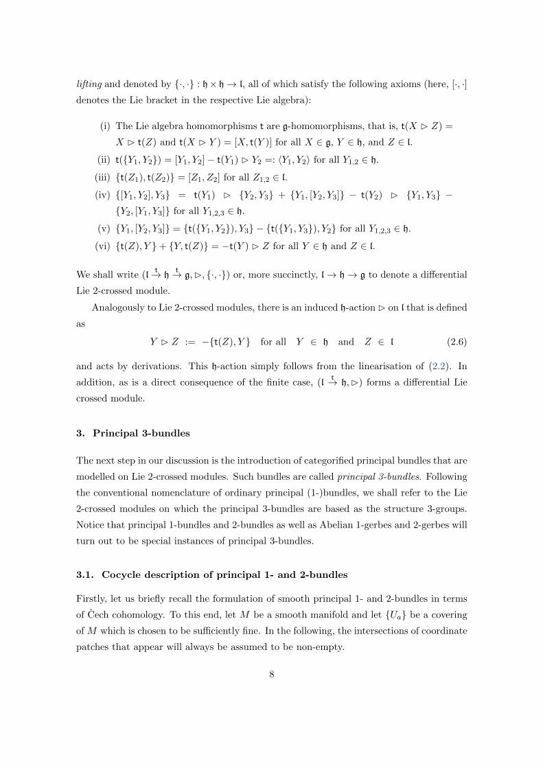
2-form, since these shifted forms represent equally good solutions to the Riemann–Hilbert

problems (4.15), (4.17), and (4.22). The combination of these transformations then yields

aa 7→ aa := g−1aag + g−1dπ1g , (4.28a)

b′a 7→ b′a := g−1 B b′a + Λπ1 + t(Θa) , (4.28b)

c′a 7→ c′a := g−1 B c′a − dπ1Θa − aa B Θa + 12 t(b

′a − Λπ1) B Θa +

+ 12b′a,Λπ1 − 1

2Λπ1 , b′a+ Σπ1 . (4.28c)

Some lengthy algebraic manipulations show that under these transformations, the relative

connection forms (4.18), (4.23), and (4.24) behave as

Aπ1 7→ Aπ1 := g−1Aπ1g + g−1dπ1g − t(Λπ1) , (4.29a)

Bπ1 7→ Bπ1 := g−1 B Bπ1 − ∇π1Λπ1 − 12 t(Λπ1) B Λπ1 − t(Σπ1) , (4.29b)

Cπ1 7→ Cπ1 := g−1 B Cπ1 − ∇0π1

(Σπ1 − 1

2Λπ1 ,Λπ1)

+

+ Bπ1 ,Λπ1+ Λπ1 , Bπ1+ Λπ1 , ∇π1Λπ1 + 12 [Λπ1 ,Λπ1 ] , (4.29c)

where we have used the abbreviations

∇π1 := dπ1 + Aπ1 B and ∇0π1 := dπ1 +

(Aπ1 + t(Λπ1)

)B . (4.29d)

We shall refer to the transformations (4.29) as gauge transformations of the relative con-

nective structure. We will demonstrate momentarily that these transformations will cor-

respond to certain space-time gauge transformations. The gauge transformations (4.29)

then imply that a pure gauge configuration is one for which the relative connection forms

are of the form

Aπ1 = g−1dπ1g − t(Λπ1) , (4.30a)

Bπ1 = −dπ1Λπ1 − (g−1dπ1g) B Λπ1 + 12 t(Λπ1) B Λπ1 − t(Σπ1) , (4.30b)

Cπ1 = −dπ1(Σπ1 + 1

2Λπ1 ,Λπ1)−

−(g−1dπ1g − t(Λπ1)

)B (Σπ1 + 1

2Λπ1 ,Λπ1)−

−

Λπ1 ,dπ1Λπ1 +(g−1dπ1g − 1

2 t(Λπ1))B Λπ1 − 1

2〈Λπ1 ,Λπ1〉. (4.30c)

This should be compared with the expressions (4.18), (4.23), and (4.24) for Aa, Ba, and

Ca, respectively, which again justifies calling a relative connective structure relative flat.

Note that the coordinate-patch-dependent Θa-transformations appearing in (4.28) drop

out of (4.29) as they should since the relative connection forms are globally defined. At

this point we would like to point out that there are additional transformations that leave

21

the splitting (4.9) invariant. They are

ga 7→ ga := gat(ha) , (4.31a)

hab 7→ hab := (ga B hah−1b )hab , (4.31b)

`abc 7→ ˜abc :=

[(gab B h−1bc )h−1ab (ga B h−1c hb)

]Bhab, (t(h

−1ab )ga) B hbh

−1c

`abc (4.31c)

for some smooth functions ha : Ua → H, and we will come back to them in Section

5. However, also these coordinate-patch-dependent transformations necessarily leave the

global relative connection forms Aπ1 , Bπ1 , and Cπ1 invariant. Thus, the freedom in defining

the relative connection forms is given by g ∈ H0(F 9|8n,G), Λπ1 ∈ H0(F 9|8n,Ω1π1 ⊗ h), and

Σπ1 ∈ H0(F 9|8n,Ω2π1 ⊗ l).

The induced transformations of the associated curvature forms (4.25a), (4.25b), and

(4.27) read as

Fπ1 7→ Fπ1 := g−1Fπ1g − t(∇π1Λπ1 + 1

2 t(Λπ1) B Λπ1), (4.32a)

Hπ1 7→ Hπ1 := g−1 B Hπ1 −(Fπ1 − t(Bπ1)

)B Λπ1 +

+ t[− ∇0

π1

(Σπ1 − 1

2Λπ1 ,Λπ1)

+

+ Bπ1 ,Λπ1+ Λπ1 , Bπ1+

+ Λπ1 , ∇π1Λπ1 + 12 [Λπ1 ,Λπ1 ]

], (4.32b)

Gπ1 7→ Gπ1 := g−1 B Gπ1 −(Fπ1 − t(Bπ1)

)B(Σπ1 − 1

2Λπ1 ,Λπ1)

+

+ Λπ1 , Hπ1 − t(Cπ1) − Hπ1 − t(Cπ1),Λπ1 −

−Λπ1 ,(Fπ1 − t(Bπ1)

)B Λπ1 . (4.32c)

The first two equations imply that the fake curvature relations (4.25) behave covariantly un-

der gauge transformations, that is, Fπ1 = t(Bπ1) and Hπ1 = t(Cπ1). In addition, provided

that these equations hold, the transformation law of the 4-form curvature Gπ1 simplifies to

Gπ1 7→ Gπ1 = g−1 B Gπ1 . This behaviour under gauge transformations explains our defin-

ition (4.27) of Gπ1 . Note that since Gπ1 = 0 also Gπ1 = 0 confirming again the consistency

of our constructions.

Field expansions. In the final step of our Penrose–Ward transform, we wish to push

down to chiral superspace M6|8n the bundle E → F 9|8n and its relative connective struc-

ture. This amounts to ‘integrating out’ the P3-dependence in the relative connection forms

stemming from the fibres of π2 : F 9|8n →M6|8n.17 Eventually, we will obtain a holomorphic

17Technically speaking, we compute the zeroth direct images of the sheaf Ωrπ1as in [3].

22

principal 3-bundle E′ → M6|8n (which is holomorphically trivial as M6|8n has trivial to-

pology) with a connective structure that is subjected to certain (superspace) constraints.

That is, certain components of the associated curvature forms on E′ will vanish.

Concretely, the relative connection forms (Aπ1 , Bπ1 , Cπ1) and the associated curvature

forms (Fπ1 , Hπ1 , Gπ1) are expanded as

Aπ1 = e[AλB]AAB + eAI A

IA , (4.33a)

Bπ1 = −14eA ∧ eBλC ε

ABCDBDEλE + 1

2eAλB ∧ eEI ε

ABCD BCDIE +

+ 12eAI ∧ eBJ BIJ

AB , (4.33b)

Cπ1 = −13eA ∧ eB ∧ eCλDε

ABCD CEFλEλF −

− 14eA ∧ eBλC ε

ABCD ∧ eEI (CDF IE)0λF +

+ 14eAλB ∧ e

EI ∧ eFJ εABCD (CCD

IJEF )0 +

+ 16eAI ∧ eBJ ∧ eCK CIJKABC (4.33c)

and

Fπ1 = −14eA ∧ eBλC ε

ABCDFDEλE + 1

2eAλB ∧ eEI ε

ABCD FCDIE +

+ 12eAI ∧ eBJ F IJAB , (4.34a)

Hπ1 = −13eA ∧ eB ∧ eCλDε

ABCDHEFλEλF −

− 14eA ∧ eBλC ε

ABCD ∧ eEI (HDF IE)0λF +

+ 14eAλB ∧ e

EI ∧ eFJ εABCD (HCD

IJEF )0 +

+ 16eAI ∧ eBJ ∧ eCK HIJK

ABC , (4.34b)

Gπ1 = −13eA ∧ eB ∧ eCλDε

ABCD ∧ eEI (GFGIE)0λFλG −

− 14eA ∧ eBλC ε

ABCD ∧ eEI ∧ eFJ (GDGIJEF )0λG +

+ 14eAλB ∧ e

EI ∧ eFJ ∧ eGK εABCD (GCD

IJKEFG)0 +

+ 16eAI ∧ eBJ ∧ eCK ∧ eDL GIJKLABCD , (4.34c)

as (Aπ1 , Bπ1 , Cπ1) and (Fπ1 , Hπ1 , Gπ1) are of homogeneity zero in the λA coordinates. Here,

we have used the relative differential 1-forms eA and eAI , which were introduced in (4.10). In

addition, the component (CABIC)0 of Cπ1 represents the totally trace-less part of CA

BIC and

(CABIJCD)0 denotes the part of CAB

IJCD that does not contain terms proportional to εABCD.

Similar conventions have been used for the components of Hπ1 and Gπ1 . We would like to

emphasise that all λ-dependence has been made explicit in the above expansions, that is,

the component fields in (4.33) and (4.34) are superfields defined on the chiral superspace

M6|8n.

23

To clarify the meaning of these component fields, we recall the components of general

low-degree differential forms on M6|8n. In the following, (·) and [·] denote symmetric

and antisymmetric indices, respectively. Note that ‘fermionic’ index pairs (IA) etc. always

appear totally symmetrised. A 1-form A on M6|8n has the components(A[AB] = 1

2εABCDA[CD] , AIB

)(4.35a)

in spinor notation while a differential 2-form B has the components(BA

B , B[AB]IC , BIJ

AB

), (4.35b)

where BAB is trace-less, and a differential 3-form C has the spinor components(

C(AB) , C(AB) , CA

BIC , C[AB]

IJCD , CIJKABC

), (4.35c)

where CABIC is trace-less over the AB indices. The C(AB)-component represents the self-

dual part of the purely bosonic components of C while the C(AB)-component represents

the anti-self-dual part, respectively. A differential 4-form D has the following spinor com-

ponents:

(DA

B , D(AB)IC , D(AB)I

C , DABIJCD , D[AB]

IJKCDE , DIJKL

ABCD

), (4.35d)

where DAB and DA

BIJCD are trace-less over the AB indices. Hence, the component fields

in (4.33) and (4.34) are nothing but the spinor components of certain differential-form-

fields on M6|8n. We thus see that the components of the relative connection forms Aπ1

and Bπ1 correspond to connection forms A and B on a holomorphically trivial principal

3-bundle E′ → M6|8n. However, as is apparent from (4.35), we do not obtain all possible

components of a connection 3-form C from the expansion (4.33). In fact, from Cπ1 we only

obtain the components CAB, (CABIC)0, (CAB

IJCD)0, and CIJKABC . We shall denote the 3-form

on M6|8n that contains only those components by C0. The ‘missing’ components in the

field expansions of the relative curvature forms (4.34) will shortly be seen as part of the

constraint equations which the curvature forms F := dA+ 12 [A,A], H := dB+A B B, and

G := dC0 + A B C0 + B,B associated with the connective structure (A,B,C0) have to

obey.

Constraint equations on chiral superspace. So far, we have obtained a holomorph-

ically trivial principal 3-bundle E′ →M6|8n over chiral superspace with a connective struc-

ture that is represented by the connection forms A, B, and C0 given by the components

fields of the expansions (4.33). Because the relative fake curvatures defined in equation

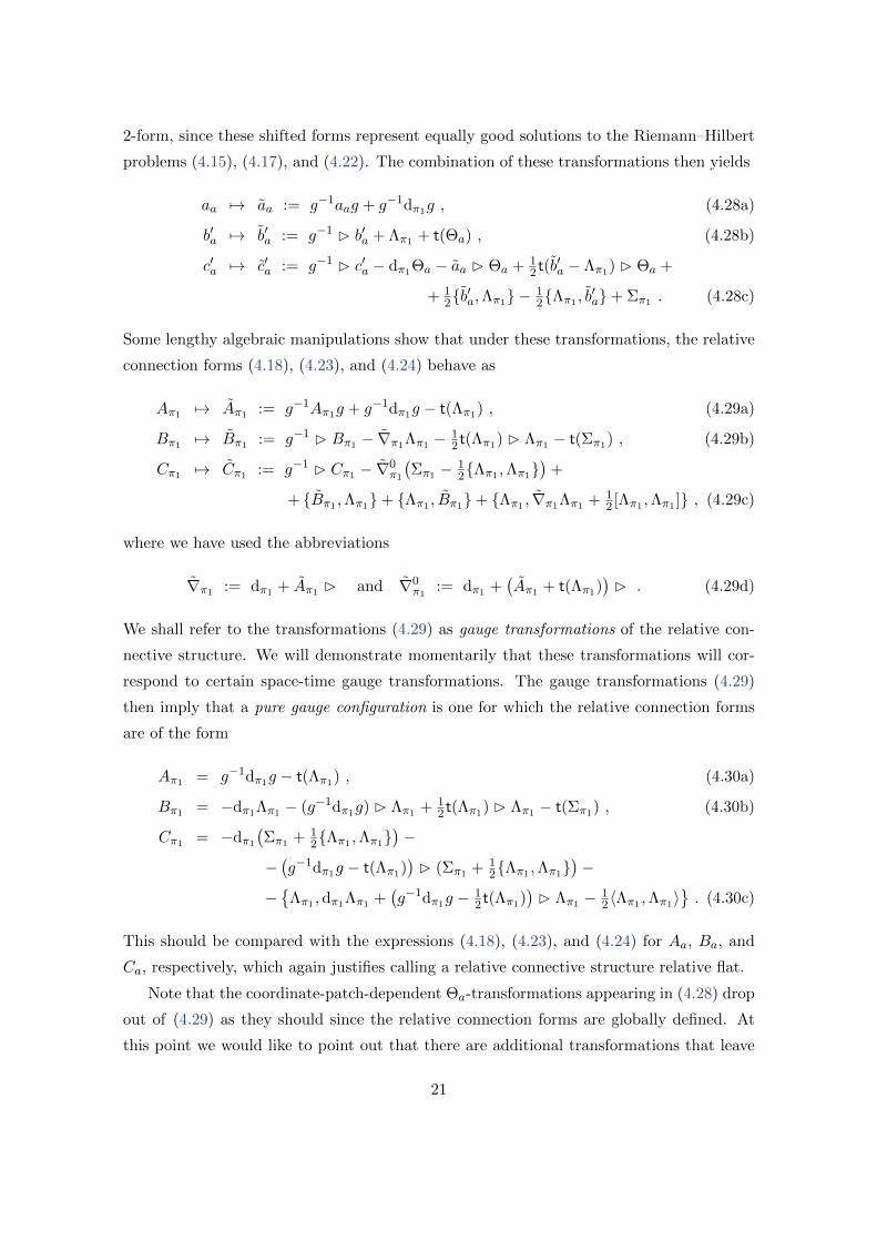
24

(4.25) and the relative 4-form curvature Gπ1 vanish, certain components of the associated

curvature forms F , H, and G will vanish. Concretely, the connective structure (A,B,C0)

on E′ →M6|8n is subject to the following set of superspace constraint equations:

FAB = t(BA

B) , FABIC = t(BAB

IC) , F IJAB = t(BIJ

AB) , (4.36a)

and

HAB = t(CAB) , (HABIC)0 = t

((CA

BIC)0),

(HABIJCD)0 = t

((CAB

IJCD)0

), HIJK

ABC = t(CIJKABC) ,(4.36b)

and

(GABIC)0 = 0 , (GABIJCD)0 = 0 , (GAB

IJKCDE)0 = 0 , GIJKLABCD = 0 . (4.36c)

The totally ‘trace-less parts’ (HABIC)0 and (HAB

IJCD)0 of the component of the curvature

3-form H may be written as

(HABIC)0 = HA

BIC − (δBCψ

IA − 1

4δBAψ

IC) , (4.37a)

(HABIJCD)0 = HAB

IJCD − εABCDφIJ , (4.37b)

where the fermionic (Graßmann-odd) ψIA and bosonic (Graßmann-even) φIJ = −φJI fields

represent the ‘trace-parts’. These fields will turn out later to be the fermions and the

scalars of the tensor multiplet. Using these expressions, the constraint equations (4.36b)

thus take the equivalent form

HAB = t(CAB) , (4.38a)

HABIC = δBCψ

IA − 1

4δBAψ

IC + t

((CA

BIC)0), (4.38b)

HABIJCD = εABCDφ

IJ + t((CAB

IJCD)0

), (4.38c)

HIJKABC = t(CIJKABC) . (4.38d)

The components of the curvatures F and H appearing in the constraint equations

25

(4.36a) and (4.38) read explicitly as

FAB = ∂BCACA − ∂CAABC + [ABC , ACA] , (4.39a)

FABIC = ∂ABA

IC −DI

CAAB + [AAB, AIC ] , (4.39b)

F IJAB = DIAA

JB +DJ

BAIA + [AIA, A

JB] + 4ΩIJAAB , (4.39c)

HAB = ∇C(ABCB) , (4.39d)

HABIC = ∇ICBAB −∇DBBDAIC +∇DABDBI

C , (4.39e)

HABIJCD = ∇ABBIJ

CD −∇ICBABJD −∇JDBABIC −

− 2ΩIJ(εABF [CBD]F − εCDF [ABB]

F ) , (4.39f)

HIJKABC = ∇IABJK

BC +∇JBBIKAC +∇KCBIJ

AB +

+ 4ΩIJBABKC + 4ΩIKBAC

JB + 4ΩJKBBC

IA . (4.39g)

These equations follow from (4.25) and the expansions (4.33) and (4.34) together with the

relations (4.11); these components also follow directly from the expressions F = dA +12 [A,A] and H = dB +A B B on chiral superspace. The self-dual part HAB of the 3-form

curvature is then given by

HAB := ∇C(ABB)C . (4.40)

The ‘trace-less parts’ (GABIC)0, (GABIJCD)0, and (GABIJKCDE)0 of the components of the

curvature 4-form G may be written as

(GABIC)0 = GABIC − χI(AδB)C , (4.41a)

(GABIJCD)0 = GA

BIJCD −

(U IJA[Cδ

BD] + 1

4δABU

IJ[CD]

)−(V IJA(Cδ

BD) −

14δABV

IJ(CD)

), (4.41b)

(GABIJKCDE)0 = GAB

IJKCDE − εABCDψIJKE −

− 5 terms to totally symmetrise in (IA)(JB)(KC ) , (4.41c)

where χIA and ψIJKA = ψ[IJ ]KA are fermionic (Graßmann-parity odd) and U IJAB = U

[IJ ]AB and

V IJAB = V

(IJ)AB are bosonic (Graßmann-parity even) which represent the ‘trace-parts’. The

bi-spinor U IJAB can be decomposed into a vector U IJ[AB] and a self-dual 3-form U IJ(AB) and

similarly for V IJAB. Thus, the constraint equations (4.36c) read as

GABIC = χI(AδB)C , GAB

IJKCDE = εABCDψ

IJKE + symmetrisation ,

GIJKLABCD = 0 , GABIJCD =

(U IJA[Cδ

BD] + 1

4δABU

IJ[CD]

)+(V IJA(Cδ

BD) −

14δABV

IJ(CD)

) (4.42)

26

with the curvature components given by18

GABIC = −∇ICCAB + 14∇

D(A(CDB)IC)0 −

− 14BD

(A, BB)DIC+ 1

4BD(AI

C , BDB) , (4.43a)

GABIJCD = 1

2

[(∇IC(CA

BJD)0 − 8ΩIJεACDEC

EB −

−BEBIC , BEA

JD+ BEAJD, BEBI

C+ (IC)↔ (JD))−

−∇EB(CEAIJCD)0 +∇EA(CEBIJCD)0 +

+ BAB, BIJCD+ BIJ

CD, BAB], (4.43b)

GABIJKCDE = 13

[∇ABCIJKCDE +

+(−∇IC(CABJKDE)0 + 8ΩIJδ

[A[C(CD]

B]KE )0 +

+ BABIC , B

JKDE+ BJK

DE , BABI

C+

+ (IC)↔ (JD) + (IC)↔ (KE ))]

, (4.43c)

GIJKLABCD = 14!

[−∇IACJKLBCD + 3

2ΩIJ(CABKLCD)0 + 3

2BIJAB, B

KLCD+

+ 23 terms to totally symmetrise in (IA)(JB)(KC )(LD)]. (4.43d)

In deriving these equations, we have again made use of (4.11). Note that one can show

that all these components of G lie in the kernel of t.

Gauge freedom on chiral superspace. Because of (4.29), there is a gauge freedom in

the above constraint equations. In particular, the gauge parameters Λπ1 and Σπ1 appearing

in the gauge transformations (4.29) of the relative connective structure are expanded as

Λπ1 = e[AλB] ΛAB + eABI λA ΛIB , (4.44a)

Σπ1 = −14eA ∧ eBλC ε

ABCDΣDEλE + 1

2eAλB ∧ eEFI λE ε

ABCD ΣCDIF +

+ 12eCAI λC ∧ eDBJ λD ΣIJ

AB , (4.44b)

where ΣAB is trace-less. Note that g in (4.29) is a globally defined, holomorphic G-valued

function on the correspondence space, and, as such, it does not depend on the coordinates

λA (since P3 is compact). Thus, g descents down to M6|8n directly.

The coefficient functions of Λπ1 and Σπ1 together with g are the gauge parameters on

M6|8n: upon substituting the expansions (4.44) and (4.33) into the transformations (4.29),

18Recall that G = dC0 +A B C0 + B,B.

27

we find the following gauge transformation on chiral superspace M6|8n:

AAB 7→ AAB := g−1AABg + g−1∂ABg − t(ΛAB) , (4.45a)

AIA 7→ AIA := g−1AIAg + g−1DIAg − t(ΛIA) , (4.45b)

BAB 7→ BA

B := g−1 B BAB − ∇BCΛCA + ∇CAΛBC −

− 12 t(Λ

BC) B ΛCA + 12 t(ΛCA) B ΛBC − t(ΣA

B) , (4.45c)

BABIC 7→ BAB

IC := g−1 B BAB

IC − ∇ABΛIC + ∇ICΛAB −

− 12 t(ΛAB) B ΛIC + 1

2 t(ΛIC) B ΛAB − t(ΣAB

IC) , (4.45d)

BIJAB 7→ BIJ

AB := g−1 B BIJAB − ∇IAΛJB − ∇JBΛIA − 4ΩIJΛAB −

− 12 t(Λ

IA) B ΛJB − 1

2 t(ΛJB) B ΛIA − t(ΣIJ

AB) , (4.45e)

CAB 7→ CAB := g−1 B CAB − ∇0C(A(ΣC

B) − 12Λ

B)D,ΛDC+ 12ΛDC ,Λ

B)D)−

−BC (A,ΛB)C+ ΛC(A, BCB)+

+ ΛC(A, ∇B)DΛDC − ∇DCΛB)D + [ΛB)D,ΛDC ] , (4.45f)

(CABIC)0 7→ (CA

BIC)0 := g−1 B (CA

BIC)0 −

−[∇0 IC

(ΣA

B − 12Λ

BC ,ΛCA+ 12ΛCA,Λ

BC)

+

+ ∇0DB(ΣDA

IC − 1

2ΛDA,ΛIC+ 1

2ΛIC ,ΛDA

)+

+ ∇0DA

(ΣDBI

C − 12Λ

DB,ΛIC+ 12Λ

IC ,Λ

DB)−

−BAB,ΛIC − ΛIC , BAB+ BDAIC ,ΛDB − ΛDB, BDAIC+

+ BDBIC ,ΛDA − ΛDA, BDBI

C −

−ΛIC , ∇BDΛDA − ∇DAΛBD + [ΛBD,ΛDA]]0, (4.45g)

(CABIJCD)0 7→ (CAB

IJCD)0 := g−1 B (CAB

IJCD)0 −

−[∇0AB

(ΣIJCD − 1

2ΛIC ,Λ

JD − 1

2ΛJD,Λ

IC)−

−∇0 IC

(ΣAB

JD − 1

2ΛAB,ΛJD+ 1

2ΛJD,ΛAB

)−

−∇0 JD

(ΣAB

IC − 1

2ΛAB,ΛIC+ 1

2ΛIC ,ΛAB

)−

− 2ΩIJεABF [C

(ΣD]

F + 12Λ

FG,ΛB]G − 12ΛD]G,Λ

AG)

+

+ 2ΩIJεCDF [A

(ΣB]

F + 12Λ

FG,ΛB]G − 12ΛB]G,Λ

AG)−

−BIJCD,ΛAB − ΛAB, BIJ

CD − BABJD,ΛIC+ ΛIC , BABJD −

−BABIC ,ΛJD+ ΛJD, BABIC −

−ΛAB, ∇ICΛJD + ∇JDΛIC − 4ΩIJΛCD + [ΛIC ,ΛJD]+

+ ΛIC , ∇ABΛJD − ∇JDΛAB + [ΛAB,ΛIC ]+

+ ΛJD, ∇ABΛIC − ∇ICΛAB + [ΛAB,ΛJD]]0, (4.45h)

28

CIJKABC 7→ CIJKABC := g−1 B CIJKABC +

−∇0 IA

(ΣJKBC − 1

2ΛJB,Λ

KC − 1

2ΛKC ,Λ

JB)

+

−∇0 JB

(ΣIKAC − 1

2ΛIA,Λ

KC − 1

2ΛKC ,Λ

IA)

+

−∇0KC

(ΣIJAB − 1

2ΛIA,Λ

JB − 1

2ΛJB,Λ

IA)

+

− 4ΩIJ(ΣAB

KC − 1

2ΛAB,ΛKC + 1

2ΛKC ,ΛAB

)+

− 4ΩIK(ΣAC

JB − 1

2ΛAC ,ΛBJ + 1

2ΛJB,ΛAC

)+

− 4ΩJK(ΣBC

IA − 1

2ΛBC ,ΛIA+ 1

2ΛIA,ΛBC

)+

+ BIJAB,Λ

KC + ΛKC , BIJ

AB −

+ BIKAC ,Λ

JB+ ΛJB, BIK

AC −

+ BJKBC ,Λ

IA+ ΛIA, BJK

BC −

−ΛIA, ∇JBΛKC + ∇KC ΛJB + 4ΩJKΛBC + [ΛJB,ΛKC ] −

−ΛJB, ∇IAΛKC + ∇KC ΛIA + 4ΩIKΛAC + [ΛIA,ΛKC ] −

−ΛKC , ∇IAΛJB + ∇JBΛIA + 4ΩIJΛAB + [ΛIA,ΛJB] . (4.45i)

4.4. Discussion of the constraint equations

To summarise the discussion of the previous section, by starting from an M6|8n-trivial

holomorphic principal 3-bundle E over the twistor space P 6|2n, we have constructed a holo-

morphically trivial principal 3-bundle over chiral superspace M6|8n that comes equipped

with a holomorphic connective structure subjected to the superspace constraint equations

(4.36a), (4.38), and (4.42). In particular, the Cech equivalence class of any such bundle

over the twistor space gives a gauge equivalence class of complex holomorphic solutions

to these constraint equations. The inverse of this Penrose–Ward transform is well-defined,

and returns an M6|8n-trivial holomorphic principal 3-bundle E′ over the twistor space P 6|2n

that is equivalent to E. To see this, we take the components of the connective structure

on M6|8n and construct the relative connective structure using equations (4.33). The fact

that the relative 4-form curvature as well as the relative fake curvatures vanish, implies

that the relative connective structure is pure gauge. From this observation, the reverse

construction of the Cech cocycles describing the principal 3-bundle E′ over twistor space

is essentially straightforward. We may therefore formulate the following theorem:

29

Theorem 4.1. There is a bijection between

(i) equivalence classes of M6|8n-trivial holomorphic principal 3-bundles over the

twistor space P 6|2n and

(ii) gauge equivalence classes of (complex holomorphic) solutions to the constraint

equations (4.36) on chiral superspace M6|2n.

Let us now discuss the constraint equations (4.36), or, equivalently, (4.36a), (4.38), and

(4.42) in more detail. The equation HAB = t(CAB) appearing in (4.38) fixes the anti-

self-dual part of HAB.19 However, by inspecting (4.45f), we realise that we have, in fact,

enough gauge freedom to choose a gauge via the gauge transformation (4.45f) in which

CAB vanishes identically. Alternatively, this also follows from an analogous cohomological

discussion to that presented in the Abelian case in [5,3]. This gauge makes then transparent

that our constraint equations indeed contain a non-Abelian generalisation of the self-dual

tensor multiplet represented by (HAB, ψIA, φ

IJ), where HAB was defined in (4.40) and the

spinors ψIA and scalars φIJ were given in (4.37).

Note that, by construction, the fields (HAB, ψIA, φ

IJ) take values in the kernel of t :

h → g. This is analogous to what was obtained previously in the context of principal

2-bundles [3]. However, it is important to realise that contrary to the principal 2-bundle

case, here this does not imply that (HAB, ψIA, φ

IJ) have to take values in the centre of the

Lie algebra h. Specifically, if, say, Y1 ∈ ker(t : h → g), then by virtue of axiom (ii) of

a differential Lie 2-crossed module, we obtain [Y1, Y2] = 〈Y1, Y2〉 6= 0, in general, for any

Y2 ∈ h. Thus, as a result of the non-triviality of the Peiffer lifting, the tensor multiplet

(HAB, ψIA, φ

IJ) obtained from principal 3-bundles is generally non-Abelian. Furthermore,

as our equations are formulated on superspace, they are manifestly supersymmetric. In

addition, the whole twistor construction is superconformal. Altogether, we have therefore

obtained N = (n, 0) manifestly superconformal, interacting field theories with n = 0, 1, 2

that contain a non-Abelian generalisation of the N = (n, 0) tensor multiplet.

We should note that a general gauge theory on a principal 3-bundle over chiral su-

perspace M6|8n, which we will discuss in Section 5, will contain the full fake curvature

condition H = H − t(C) = 0. According to our constraint equations (4.38), we do not

find the full fake curvature equation on chiral superspace. However, if, say, the sequence

l → h → g was exact at h, we could always adjust the 3-form potential C such that the

general fake curvature condition holds since, by construction, we have t(H) = 0 for the

full 3-form curvature. Otherwise, even though the relation of our constraint equations

19This is quite similar to what happens in the field equations of [15].

30

to parallel transport of two-dimensional objects remains unclear at this stage20, they still

describe a consistent superconformal gauge theory.21

A particularly interesting point is now the coupling of the ‘matter fields’, such as ψIA

and φIJ defined in (4.37), to the connective structure. Equations (4.38) together with

(4.45a)–(4.45e) show that these fields transform under gauge transformations as

ψIA 7→ ψIA := g−1 B ψIA + t(αIA) and φIJ 7→ φIJ := g−1 B φIJ + t(αIJ) , (4.46)

where the gauge parameters αIA and αIJ are fixed by the gauge parameters Λ and Σ entering

(4.45a)–(4.45e). This is the desired transformation and such a coupling of matter fields to

a connective structure of higher gauge theory had only been obtained in [8] so far. Notice

that HAB transforms likewise as HAB 7→ HAB := g−1 B HAB + t(αAB).

Finally, let us come to a few special cases of our construction. First of all, if we

reduce our principal 3-bundle to a principal 2-bundle by choosing a Lie 2-crossed module

1 → H → G, our equations reduce to those obtained in [8]. A further reduction to

the Abelian case 1 → U(1) → 1 then obviously leads to the situation described

in [3, 4]. One can also perform the Penrose–Ward transform for principal 3-bundles over

the hyperplane twistor space introduced in [3]. This will yield solutions to non-Abelian

generalisations of the self-dual string equations. As the discussion is straightforward (cf.

the discussion for principal 2-bundles in [8]), we refrain from going into any further details.

4.5. Constraint equations and superconformal field equations

A detailed analysis of our constraint equations requires to reduce them to an equivalent

set of field equations on six-dimensional space-time M6. This step is well understood e.g.

for the constraint equations of maximally supersymmetric Yang–Mills theories [47] and

three-dimensional supersymmetric Chern–Simons theories [48].

In this reduction, the components of the curvatures along fermionic directions are iden-

tified with matter superfields as done above, and the Bianchi identities yield the corres-

ponding field equations for a supermultiplet of superfields. These field equations can then

be shown to be equivalent to the field equations restricted to the purely bosonic part of

the superfields. One thus arrives at a set of supersymmetric field equations on ordinary

space-time. This reduction procedure, however, is very involved, and it is therefore beyond

the scope of this paper and postponed to future work.

20Note that parallel transport requires the vanishing of fake curvatures, see [45,22].21In [46] a (non-supersymmetric) higher gauge theory including an action principle based on principal

2-bundles was obtain that does not require the vanishing of the fake curvature either.

31

Although we do not have the explicit field equations on space-time, we already know

that they will consist of a N = (2, 0) superconformal higher gauge theory involving a

connective structure on a trivial principal 3-bundle over six-dimensional Minkowski space.

Recall that recently, N = (1, 0) superconformal field theories were derived from a non-

Abelian generalisation of the tensor hierarchy [15, 17, 19]. An obvious question is now if

there is any relation between our N = (2, 0) field equations and those of the (1, 0)-models.

The general relation between higher gauge theories and the (1, 0)-models was explored

in [49]. There it was found that the algebraic structure underlying the (1, 0)-models can

be encoded in a certain class of semistrict Lie n-algebras. Moreover, the field equations

are those of a higher gauge theory with an additional six-dimensional vector multiplet

coupled to the tensor multiplet. In [15,17,19], however, no fake curvature conditions were

imposed and correspondingly, there is no underlying parallel transport of extended objects.

A further difference to our superconformal field equations is the fact that we had to restrict

our discussion to the case of strict Lie n-algebras, as a more general cocycle description

of principal 3-bundles is not yet available. We thus see that there is a large overlap in

field content and equations of motion between our superconformal field equations and the

(1, 0)-models.

Finally, it is certainly tempting to speculate about the role of our constraint equations

in the description of systems of multiple M5-branes. Recall that the interactions of M5-

branes are mediated by M2-branes suspended between these, and their boundaries form

so-called self-dual strings. An effective description of M5-branes should therefore capture

the parallel transport of these self-dual strings, just as the effective description of D-branes

by Yang–Mills theories captures the parallel transport of the endpoints of strings. This

argument directly leads to superconformal higher gauge theories such as the one constructed

in this paper.

Possibly the most important consistency check for an effective description of M5-branes

is a convincing reduction mechanism to five-dimensional supersymmetric Yang–Mills the-

ory. This remains an open problem for both our field equations as well as those of the

(1, 0)-model. Similarly unclear is what higher gauge group one should choose for a descrip-

tion of systems of multiple M5-branes. There are arguments which are based on a relation

of higher principal bundles with principal bundles on loop space and the necessity of a

reduction to five-dimensional Yang–Mills theory. Naively, they suggest to use the auto-

morphism 2-group of U(N). More sophisticated arguments suggest to use string 2-groups,

cf. [13].

32

5. Higher gauge theory on principal 3-bundles

In the derivation of the constraint equations in the last section, all features of gauge theory

on principal 3-bundles have become apparent. Let us summarise these in the following.

To give a complete description, we will discuss the underlying non-Abelian differential

cohomology right from the start. Recall that Abelian (n−1)-gerbes with connective struc-

ture are described by Deligne cohomology [50]. The non-Abelian differential cohomology

we have in mind here is one that is based on principal n-bundles with structure n-groups,

and which reduces to Deligne cohomology for the case of Abelian (n − 1)-gerbes, that

is principal n-bundles with gauge n-group Bn−1U(1). In the following, we shall iterate

through the principal n-bundles for n = 0, 1, 2, 3.

Consider a manifold M with a cover U := Ua. We denote Cech p-cochains that take

values in the sheaf of smooth functions into G by Cp,0(U,G) and Cech p-cochains that take

values in the sheaf of differential q-forms on M times a Lie algebra g by Cp,q(U, g).

Degree 0. A degree-0 cochain ga with values in G is specified by a set ga ∈ C0,0(U,G).

The cocycle condition reads as

ga = gb on Ua ∩ Ub . (5.1)

As usual in degree 0, there is no equivalence between cocycles in terms of coboundaries.

Thus, an element of the degree 0 cohomology set defines a smooth function M → G, which

could be called a principal 0-bundle.

Degree 1. A degree-1 G-valued cochain (gab, Aa) is given by the Cech cochains

gab ∈ C1,0(U,G) and Aa ∈ C0,1(U, g). The degree-1 cocycle condition amounts to

gac = gabgbc on Ua ∩ Ub ∩ Uc , (5.2a)

Ab = g−1ab Aagab + g−1ab dgab on Ua ∩ Ub . (5.2b)

Two degree-1 cocycles (gab, Aa) and (gab, Aa) are considered equivalent if there is

a degree-0 cochain ga with values in G such that

Aa = g−1a Aaga + g−1a dga on Ua , (5.3a)

gab = g−1a gabgb on Ua ∩ Ub . (5.3b)

We conclude that elements of the degree-1 cohomology set define principal (1-)bundles

with connection. Note that the second cocycle condition turns the local Lie algebra valued

33

one-forms Aa into a global object, the connection. The curvature of (gab, Aa) ,

Fa := dAa + 12 [Aa, Aa] , (5.4)

fulfils the Bianchi identity dFa + [Aa, Fa] = 0. Moreover, the curvatures of (gab, Aa)and (gab, Aa) are related via

Fa = g−1a Faga on Ua . (5.5)

Degree 2. A degree-2 cochain with values in the Lie crossed module (Ht→ G) consists

of the following Cech cochains:

habc ∈ C2,0(U,H) , Λab ∈ C1,1(U, h) , Ba ∈ C0,2(U, h) ,

gab ∈ C1,0(U,G) , Aa ∈ C0,1(U, g) .(5.6)

Note that contrary to Deligne cohomology, the sum of Cech and de Rham degrees of the

Cech cochains forming the non-Abelian differential cochain will no longer be constant from

now on. The degrees are constant, however, across the form-valued Cech cochains which

take values in the same Lie algebra or integrating Lie group. Moreover, since we fixed our

conventions such that gaa = 1, we do not have the additional elements C0,0(U,H) that

appeared in Schreiber & Waldorf [51]. The degree-2 cocycle conditions are

hacdhabc = habd(gab B hbcd) , (5.7a)

Λac = Λbc + g−1bc B Λab − g−1ac B (habc∇ah−1abc) , (5.7b)

Bb = g−1ab B Ba −∇bΛab − 12 [Λab,Λab] , (5.7c)

gac = t(habc)gabgbc , (5.7d)

Ab = g−1ab Aagab + g−1ab dgab − t(Λab) , (5.7e)

where each equation is considered on the obvious intersections of patches. Note that upon

putting haba = 1, the cocycle condition for Λab turns into the corresponding consistency

condition given in [1].

Two cocycles (habc, Λab, Ba, gab, Aa) and (habc, Λab, Ba, gab, Aa)are considered cohomologous, if there is a degree-1 (H

t→ G)-valued cochain

hab ∈ C1,0(U,H) , Λa ∈ C0,1(U, h) and ga ∈ C0,0(U,G) (5.8)

34

such that

habc = g−1a B (hachabc(gab B h−1bc )h−1ab ) , (5.9a)

Λab = g−1b B Λab + Λb − g−1ab B Λa − (g−1b g−1ab ) B (h−1ab ∇bhab) , (5.9b)

Ba = g−1a B Ba − ∇aΛa − 12 [Λa,Λa] , (5.9c)

gab = g−1a t(hab)gabgb , (5.9d)

Aa = g−1a Aaga + g−1a dga − t(Λa) . (5.9e)

On each patch Ua, we introduce the curvatures

Fa := dAa + 12 [Aa, Aa] and Ha := dBa +Aa B Ba = ∇aBa . (5.10)

To render the underlying parallel transport of one-dimensional objects along surfaces re-

parameterisation invariant, one has to impose the fake curvature condition:

Fa := Fa − t(Ba) = 0 . (5.11)

Besides the Bianchi identity for Fa, the fake curvature condition yields the Bianchi identity

dHa +Aa B Ha = 0 together with

t(Ha) = 0 , (5.12)

and this equation, together with the Peiffer identity, implies that Ha takes values in the

centre of h. The curvatures of cohomologous 2-cochains (habc, Λab, Ba, gab, Aa)and (habc, Λab, Ba, gab, Aa) are related as follows:

Fa = g−1a Faga − t(∇aΛa + 12 [Λa,Λa]) , (5.13a)

Ha = g−1a B Ha − (Fa − t(Ba)) B Λa . (5.13b)

Note that the degree-2 cohomology set arose from the degree-1 set by categorification:

the cocycle and coboundary relations for degree 1 hold in degree 2 only up to isomorphisms.

Therefore we expect that beyond the equivalence relation between cochains, there should be

an equivalence relation between equivalence relations. Two degree-0 cochains (ga, hab)and (ga, hab) encoding an equivalence relation (5.9) are called cohomologous, if there

is a degree-0 cochain ha ∈ C0,0(U, h) such that

ga = t(ha)ga and hab = hahab(gab B h−1b ) . (5.14)

35

Degree 3. Degree-3 cochains with values in the Lie 2-crossed module (Lt→ H

t→ G) are

encoded in the following Cech cochains:

`abcd ∈ C3,0(U, L) , Ξabc ∈ C2,1(U, l) , Σab ∈ C1,2(U, l) , Ca ∈ C0,3(U, l) ,

habc ∈ C2,0(U,H) , Λab ∈ C1,1(U, h) , Ba ∈ C0,2(U, h) ,

gab ∈ C1,0(U,G) , Aa ∈ C0,1(U, g) .

(5.15)

The degree-3 cocycle conditions for `abcd, habc, and gab are given in (3.5). The

corresponding equations on the gauge potentials Ca, Ba, and Aa are given by gauge

transformations across overlaps of patches:

Cb = g−1ab B Ca −∇b(Σab − 1

2Λab,Λab)

+ t(Λab) B12Λab,Λab+

+ Bb,Λab+ Λab, Bb+ Λab,∇bΛab + 12 [Λab,Λab] , (5.16a)

Bb = g−1ab B Ba −∇bΛab − 12 [Λab,Λab]− t(Σab) , (5.16b)

Ab = g−1ab Aagab + g−1ab dgab − t(Λab) . (5.16c)

The degree-3 cocycle condition for Λab is an obvious categorification of the degree-2

cocycle condition of Λab. We omit the remaining cocycle conditions for Ξabc and

Σab, as their explicit form is mostly irrelevant for working with higher gauge theories

based on principal 3-bundles. Moreover, they are easily derived: the degree-3 cocycle con-

dition for Λab and Σab are obtained by demanding consistency of the ‘gluing relations’

(5.16) across triple intersections of patches Ua ∩ Ub ∩ Uc. The consistency of the thus ob-

tained cocycle conditions across quadruple intersections of patches then yields the cocycle

condition for Ξabc.Two degree-3 cochains (`abcd, Ξabc, Σab, Ca, habc, Λab, Ba, gab, Aa)

and (˜abcd, Ξabc, Σab, Ca, habc, Λab, Ba, gab, Aa) are cohomologous, if re-

lations (3.6), the following equations:

Ca = g−1a B Ca − ∇0a

(Σa − 1

2Λa,Λa)

+

+ Ba,Λa+ Λa, Ba+ Λa, ∇aΛa + 12 [Λa,Λa] , (5.17a)

Ba = g−1a B Ba − ∇aΛa − 12 [Λa,Λa]− t(Σa) , (5.17b)

Aa = g−1a Aaga + g−1a dga − t(Λa) , (5.17c)

and additional equations for Ξabc, Σab, and Λab, which we again suppress, are satis-

fied. Here, ∇0a := d + A0

a B with A0a := A0

a + t(Λa).

Again, to have a well-defined underlying parallel transport along volumes, the curvatures

Fa := dAa + 12 [Aa, Aa] , Ha = ∇aBa , Ga := ∇aCa + Ba, Ba (5.18)

36

have to satisfy the fake curvature conditions

Fa := Fa − t(Ba) = 0 and Ha := Ha − t(Ca) = 0 . (5.19)

Besides the usual Bianchi identity involving Fa, we have

∇aHa + t(Ba, Ba) = 0 and ∇aGa = 0 (5.20)

together with

t(Ha) = 0 and t(Ga) = 0 . (5.21)

Once again, this should be compared to the principal 2-bundle case. Because of the Peiffer

lifting, the equation t(Ha) = 0 does not imply that Ha takes values in the centre of h,

rather it is non-Abelian in general. However, t(Ga) = 0 implies that Ga lies in the centre

of l since (lt→ h,B), with B being the induced h-action on l defined in (2.6), is a differential

crossed module.

The curvatures of cohomologous 3-cochains are then related via

Fa = g−1a Faga − t(∇aΛa + 1

2 t(Λa) B Λa), (5.22a)

Ha = g−1a B Ha −(Fa − t(Ba)

)B Λa +

+ t[− ∇0

a

(Σa − 1

2Λa,Λa)

+ Ba,Λa+ Λa, Ba+

+ Λa, ∇aΛa + 12 [Λa,Λa]

], (5.22b)

Ga = g−1a B Ga −(Fa − t(Ba)

)B(Σa − 1

2Λa,Λa)

+

+ Λa, Ha − t(Ca) − Ha − t(Ca),Λa −

−Λa,(Fa − t(Ba)

)B Λa . (5.22c)

Eventually, note that there are again equivalence relations between equivalence relations

here, and one has a categorified version of equation (5.14). They appear in the Penrose–

Ward transform in (4.31), but they turn out to be irrelevant for the resulting field equations,

as one would expect. Note that the has used in the categorification of (5.14) and the

ones appearing in (4.31) are related by ha ↔ g−1a B ha. In addition, there is a further

equivalence relation between these equivalences. Since these formulæ are rather lengthy,

not very illuminating and of no direct use in the discussion of the dynamics of connective

structures on principal 3-bundles, we again refrain from listing them here.

6. Conclusions

In this paper, we constructed newN = (n, 0) superconformal field theories in six dimensions

with n = 0, 1, 2 that contain a non-Abelian generalisation of the tensor multiplet. The

37

equations were obtained from a Penrose–Ward transform of certain holomorphic principal

3-bundles over a suitable twistor space. Compared to the superconformal field equations

that we had derived previously in [8], the equations here are significantly more general:

the Peiffer identity is lifted in a controlled way and the previous restriction of the 3-form

curvature H to live in the centre of a Lie algebra is removed. Moreover, our new equations

contain a 3-form potential, which can be motivated by either making connections to M-

theory or by referring to other approaches to six-dimensional superconformal field theories

as those in [15,17,19,20] or [13].

The Penrose–Ward transform exposed all features of higher gauge theory with principal

3-bundles, some of which had remained unexplored in the literature so far. In particular, we

formulated the non-Abelian differential cohomology that describes principal 3-bundles with

connective structure. This cohomology nicely reduces to the usual Deligne cohomology,

when the principal 3-bundle is reduced to an Abelian 2-gerbe.

The constraint equations we obtained seem rather promising to us, and they lead to

a number of questions that we intend to address in future work. First of all, it is im-

portant to reduce our superfield constraint equations to actual field equations on ordinary

six-dimensional space-time. This issue appears usually in the twistor description of field

equations, see [47] for the case of maximally supersymmetric Yang–Mills theory in four di-

mensions and [48] for similar expansions in the context of three-dimensional supersymmet-

ric Chern–Simons theories. Once this is done, a more detailed analysis of the field equations

and their possible relation to the effective description of M5-branes can be undertaken. In

particular, the reduction to five-dimensional super Yang–Mills theory as well as a detailed

study of the BPS configurations known as self-dual strings should be performed. As we

pointed out, our superconformal tensor field equations can be dimensionally reduced to

those of a non-Abelian generalisation of the self-dual string equations. Alternatively, these

equations can also be obtained from holomorphic principal 3-bundles over the hyperplane

twistor space introduced in [3].

An important question is the interpretation of the additional 3-form potential that is not

believed to be part of the field content of an effective description of M5-branes. Currently,

it seems that this field should be regarded analogously to the 3-form field appearing in

[15,17,19,20]. That is, it merely mediates couplings between the various other fields.

Finally, it still seems conceivable that a manageable Cech description of principal 2-

bundles with semistrict structure 2-groups exists. In this case, our twistor construction

would be an ideal approach both to explore the general definition of semistrict higher

gauge theories as well as to find new and more general superconformal field theories in six

dimensions.

38

Acknowledgements

We would like to thank D. Baraglia, D. Berman, C. S. Chu, P. Hekmati, B. Jurco, N. Lam-

bert, L. Mason, A. Mikovic, M. Murray, G. Papadopoulos, D. Roberts, D. Smith, D. Sor-

okin, and R. Vozzo for enjoyable discussions. CS was supported by an EPSRC Career

Acceleration Fellowship.

Appendix

A. Collection of Lie 2-crossed module identities and their proofs

Useful Lie 2-crossed module identities. Let us collect and prove some useful iden-

tities which are used throughout this work.

We have

1, h = 1 = h,1 for all h ∈ H , (A.1)

as follows directly from applying the Lie 2-crossed module axioms (iv) and (v) to 11, hand h,11, respectively.

Obvious, but very useful is also

`1`2 = t(`1), t(`2)`2`1 for all `1, `2 ∈ L . (A.2)

By applying the Lie 2-crossed module axiom (iv) to the expression h1h−11 , h1h2h1,we find

h1, h2−1 = t(h1) B h−11 , h1h2h−11 for all h1, h2 ∈ H . (A.3)

Together, with axiom (vi), this enables us to rewrite the induced H-action on L given in

(2.2) as

h B ` = t(h) B (`h−1, ht(`−1)h−1) for all h ∈ H and ` ∈ L . (A.4)

Note that

h1, h2` = ``−1h1, h2`(h1, h2)−1h1, h2

= `t(`)−1, t(h1, h2)h1, h2

= (t(h1, h2) B `)h1, h2 (A.5)

for all h1, h2 ∈ H and ` ∈ L.

39

As observed in [22], the fact that the action of H onto L is an automorphism together

with (A.5) implies that we can reformulate the Lie 2-crossed module axiom (v) as follows:

h1, h2h3 = h1, h2h1, h3〈h1, h3〉−1, t(h1) B h2

= h1, h2((t(h1) B h2) B h1, h3)

= (t(h1, h2) B (t(h1) B h2) B h1, h3)h1, h2

= ((h1h2h−11 (h1h

−12 h−11 )) B (h1h2h

−11 ) B h1, h3)h1, h2

= ((h1h2h−11 ) B h1, h3)h1, h2 (A.6)

for all h1, h2, h3 ∈ H.

Proof that the induced H-action is by automorphisms. To verify that the induced

H-action (2.2) is an automorphism action, one has to demonstrate the two relations h1h2 B

` = h1 B h2 B ` and h B (`1`2) = (h B `1)(h B `2) for all h, h1, h2 ∈ H and `, `1, `2 ∈ L.

To show the first relation, we use the alternative version (A.4) for the induced H-action

on L. We find

(h1h2) B ` = (t(h1h2) B `)t(h1h2) B (h1h2)−1, t(h1h2) B (h1h2t(`

−1)h−12 h−11 )

= (t(h1h2) B `)t(h1h2) B h−12 , t(h1h2) B (h2t(`−1)h−12 ) ×

×t(h1) B h−11 , t(h1) B (h1h2t(`−1)h−12 h−11

= h1 B (h2 B `) . (A.7)

To show the second relation, we consider

(h B `1)(h B `2) = `1t(`−11 ), h`2t(`−12 ), h

= `1`2t(`−12 ), t(`−11 )ht(`1)h−1t(`−11 ), ht(`−12 ), h

= `1`2t(`−12 ), t(`−11 )ht(`1)h−1 ×

×t(`−12 ), hht(`−12 )h−1t(`2), t(`−11 )ht(`1)h

−1t(`−11 ), h

= `1`2t(`−12 ), t(`−11 )ht(`1)h−1ht(`−11 ), h

= `1`2t(`−12 ), t(`−11 )ht(`1)t(`−11 ), h

= `1`2t(`−12 )t(`−11 ), h

= h B (`1`2) . (A.8)

40

References

[1] J. C. Baez and J. Huerta, An invitation to higher gauge theory, Gen. Relativ. Gravit. 43 (2011)

2335 [1003.4485 [hep-th]].

[2] M. K. Murray, A Penrose transform for the twistor space of an even-dimensional conform-

ally flat Riemannian manifold, Ann. Global Anal. Geom. 4 (1986) 71. • L. P. Hughston,

Applications of SO(8) spinors, in: ‘Gravitation and Geometry: a volume in honour of Ivor

Robinson,’ eds. W. Rindler and A. Trautman, 253, Bibliopolis, Naples, 1987. • R. Penrose

and W. Rindler, Spinors and space-time. Vol. 2: spinor and twistor methods in space-time

geometry, Cambridge University Press, Cambridge, 1986.

[3] C. Saemann and M. Wolf, On twistors and conformal field theories from six dimensions, J.

Math. Phys. 54 (2013) 013507 [1111.2539 [hep-th]].

[4] L. Mason, R. Reid-Edwards, and A. Taghavi-Chabert, Conformal field theories in six-

dimensional twistor space, J. Geom. Phys. 62 (2012) 2353 [1111.2585 [hep-th]].

[5] R. J. Baston and M. G. Eastwood, The Penrose transform, Oxford University Press (1990).

[6] L. Mason and R. Reid-Edwards, The supersymmetric Penrose transform in six dimensions,

1212.6173 [hep-th].

[7] P. Pasti, D. P. Sorokin, and M. Tonin, Note on manifest Lorentz and general coordinate invari-

ance in duality symmetric models, Phys. Lett. B 352 (1995) 59 [hep-th/9503182]. • P. Pasti,

D. P. Sorokin, and M. Tonin, Duality symmetric actions with manifest space-time symmetries,

Phys. Rev. D 52 (1995) 4277 [hep-th/9506109]. • P. Pasti, D. P. Sorokin, and M. Tonin, On

Lorentz invariant actions for chiral p-forms, Phys.Rev. D 55 (1997) 6292 [hep-th/9611100].

• P. Pasti, D. P. Sorokin, and M. Tonin, Covariant action for a D = 11 five-brane with the

chiral field, Phys. Lett. B 398 (1997) 41 [hep-th/9701037].

[8] C. Saemann and M. Wolf, Non-abelian tensor multiplet equations from twistor space, Commun.

Math. Phys. 328 (2014) 527 [1205.3108].

[9] S. Palmer and C. Saemann, M-brane models from non-Abelian gerbes, JHEP 1207 (2012) 010

[1203.5757 [hep-th]].

[10] N. Lambert and C. Papageorgakis, Non-Abelian (2,0) tensor multiplets and 3-algebras, JHEP

1008 (2010) 083 [1007.2982 [hep-th]].

[11] P. Richmond, Multiple M-branes and 3-algebras, PhD thesis, King’s College London (2012)

[1211.6930 [hep-th]].

[12] J. C. Baez, D. Stevenson, A. S. Crans, and U. Schreiber, From loop groups to 2-groups, Homol.

Homot. Appl. 9 (2007) 101 [math.QA/0504123].

[13] D. Fiorenza, H. Sati, and U. Schreiber, Multiple M5-branes, string 2-connections, and 7d

non-Abelian Chern–Simons theory, 1201.5277 [hep-th].

[14] D. Fiorenza, U. Schreiber and J. Stasheff, Cech cocycles for differential characteristic classes

– An infinity-Lie theoretic construction, Adv. Th. Math. Phys. 16 (2012) 149 [1011.4735].

41

[15] H. Samtleben, E. Sezgin, and R. Wimmer, (1,0) superconformal models in six dimensions,

JHEP 1112 (2011) 062 [1108.4060 [hep-th]].

[16] C.-S. Chu, A theory of non-Abelian tensor gauge field with non-Abelian gauge symmetry G×G,

Nucl. Phys. B 866 (2013) 43 [1108.5131 [hep-th]].

[17] H. Samtleben, E. Sezgin, R. Wimmer, and L. Wulff, New superconformal models in six dimen-

sions: gauge group and representation structure, PoS CORFU 2011 (2011) 71 [1204.0542

[hep-th]].

[18] M. Akyol and G. Papadopoulos, (1,0) superconformal theories in six dimensions and Killing

spinor equations, JHEP 1207 (2012) 070 [1204.2167 [hep-th]].

[19] H. Samtleben, E. Sezgin, and R. Wimmer, Six-dimensional superconformal couplings of non-

Abelian tensor and hypermultiplets, JHEP 1303 (2013) 068 [1212.5199 [hep-th]].

[20] I. Bandos, H. Samtleben, and D. Sorokin, Duality-symmetric actions for non-Abelian tensor

fields, Phys. Rev. D 88 (2013) 025024 [1305.1304 [hep-th]].

[21] P.-M. Ho, K.-W. Huang, and Y. Matsuo, A non-Abelian self-dual gauge theory in 5+1 dimen-

sions, JHEP 1107 (2011) 021 [1104.4040 [hep-th]]. • C.-S. Chu and S.-L. Ko, Non-Abelian

action for multiple M5-branes, JHEP 1205 (2012) 028 [1203.4224 [hep-th]]. • F. Bonetti,

T. W. Grimm, and S. Hohenegger, A Kaluza-Klein inspired action for chiral p-forms and

their anomalies, Phys. Lett. B 720 (2013) 424 [1206.1600 [hep-th]]. • C.-S. Chu, S.-L. Ko,

and P. Vanichchapongjaroen, Non-Abelian self-dual string solutions, JHEP 1209 (2012) 018

[1207.1095 [hep-th]]. • F. Bonetti, T. W. Grimm, and S. Hohenegger, Non-Abelian tensor

towers and (2, 0) superconformal theories, JHEP 1305 (2013) 129 [1209.3017 [hep-th]]. •C.-S. Chu and P. Vanichchapongjaroen, Non-Abelian self-dual string and M2-M5 branes in-

tersection in supergravity, JHEP 1306 (2013) 028 [1304.4322 [hep-th]].

[22] J. F. Martins and R. Picken, The fundamental Gray 3-groupoid of a smooth manifold and

local 3-dimensional holonomy based on a 2-crossed module, Diff. Geom. App. 29 (2011) 179

[0907.2566 [math.CT]].

[23] J. C. Baez and A. D. Lauda, Higher-dimensional algebra V: 2-groups, Th. App. Cat. 12 (2004)

423 [math/0307200].

[24] L. Breen and W. Messing, Differential geometry of gerbes, Adv. Math. 198 (2005) 732

[math.AG/0106083].

[25] D. Conduche, Modules croises generalises de longueur 2, J. Pure Appl. Algebra 34 (1984) 155.

[26] L. Breen, Notes on 1- and 2-gerbes, math.CT/0611317.

[27] K. H. Kamps and T. Porter, 2-groupoid enrichments in homotopy theory and algebra, K-Theory

25 (2002) 373.

[28] R. Brown and N. D. Gilbert, Algebraic models of 3-types and automorphism structures for

crossed modules, Proc. LMS 3 (1989) 51.

[29] P. Aschieri, L. Cantini, and B. Jurco, Non-Abelian bundle gerbes, their differential geometry

and gauge theory, Commun. Math. Phys. 254 (2005) 367 [hep-th/0312154].

42

[30] C. Wockel, Principal 2-bundles and their gauge 2-groups, Forum Math. 23 (2011) 566

[0803.3692 [math.DG]].

[31] L. Breen, On the classification of 2-gerbes and 2-stacks, Asterisque 225 (1994).

[32] B. Jurco, Non-Abelian bundle 2-gerbes, Int. J. Geom. Meth. Mod. Phys. 08 (2011) 49

[0911.1552 [math.DG]].

[33] R. S. Ward, On self-dual gauge fields, Phys. Lett. A 61 (1977) 81. • M. Atiyah and R. Ward,

Instantons and algebraic geometry, Commun. Math. Phys. 55 (1977) 117.

[34] R. Penrose, Non-linear gravitons and curved twistor theory, Gen. Rel. Grav. 7 (1976) 31. •M. Atiyah, N. J. Hitchin, and I. Singer, Self-duality in four-dimensional Riemannian geometry,

Proc. Roy. Soc. Lond. A 362 (1978) 425. • R. Ward, Self-dual space-times with cosmological

constant, Commun. Math. Phys. 78 (1980) 1.

[35] Y. I. Manin, Gauge field theory and complex geometry, Grundlehren der Mathematischen

Wissenschaften, 289, Springer, Berlin, 1988.

[36] S. A. Merkulov, Paraconformal supermanifolds and nonstandard N -extended supergravity mod-

els, Class. Quant. Grav. 8 (1991) 557. • S. A. Merkulov, Supersymmetric non-linear graviton,

Funct. Anal. Appl. 26 (1992) 72. • S. A. Merkulov, Simple supergravity, supersymmetric non-

linear gravitons and supertwistor theory, Class. Quant. Grav. 9 (1992) 2369. • S. A. Merkulov,

Quaternionic, quaternionic Kahler, and hyper-Kahler supermanifolds, Lett. Math. Phys. 25

(1992) 7.

[37] E. Witten, Perturbative gauge theory as a string theory in twistor space, Commun. Math.

Phys. 252 (2004) 189 [hep-th/0312171].

[38] A. D. Popov and C. Saemann, On supertwistors, the Penrose–Ward transform and N = 4 super

Yang–Mills theory, Adv. Theor. Math. Phys. 9 (2005) 931 [hep-th/0405123]. • N. Berkovits

and E. Witten, Conformal supergravity in twistor-string theory, JHEP 0408 (2004) 009

[hep-th/0406051]. • M. Wolf, Self-dual supergravity and twistor theory, Class. Quant. Grav.

24 (2007) 6287 [0705.1422 [hep-th]]. • L. J. Mason and M. Wolf, A twistor action for N = 8

self-dual supergravity, Commun. Math. Phys. 288 (2009) 97 [0706.1941 [hep-th]].

[39] R. Penrose, Twistor algebra, J. Math. Phys. 8 (1967) 345. • R. Penrose, Twistor quantization

and curved space-time, Int. J. Theor. Phys. 1 (1968) 61. • R. Penrose, Solutions of the zero-

rest-mass equations, J. Math. Phys. 10 (1969) 38. • R. Penrose and M. A. H. MacCallum,

Twistor theory: an approach to the quantization of fields and space-time, Phys. Rept. 6 (1972)

241.

[40] A. Ferber, Supertwistors and conformal supersymmetry, Nucl. Phys. B 132 (1978) 55.

[41] R. S. Ward, Completely solvable gauge field equations in dimension greater than four, Nucl.

Phys. B 236 (1984) 381. • A. D. Popov, Hermitian-Yang–Mills equations and pseudo-

holomorphic bundles on nearly Kahler and nearly Calabi–Yau twistor 6-manifolds, Nucl. Phys.

B 828 (2010) 594 [0907.0106 [hep-th]]. • M. Wolf, A connection between twistors and su-

perstring sigma models on coset superspaces, JHEP 0909 (2009) 071 [0907.3862 [hep-th]]. •

43

M. Wolf, Contact manifolds, contact instantons, and twistor geometry, JHEP 1207 (2012) 074

[1203.3423 [hep-th]]. • O. Lechtenfeld and A. D. Popov, Instantons on the six-sphere and

twistors, J. Math. Phys. 53 (2012) 123506 [1206.4128 [hep-th]]. • T. A. Ivanova, O. Lechten-

feld, A. D. Popov, and M. Tormaehlen, Instantons in six dimensions and twistors, Nucl. Phys.

B 882 (2014) 205 [1302.5577 [hep-th]].

[42] E. Witten, An interpretation of classical Yang–Mills theory, Phys. Lett. B 77 (1978) 394. •J. Isenberg, P. B. Yasskin, and P. S. Green, Non-self-dual gauge fields, Phys. Lett. B 78 (1978)

462. • N. P. Buchdahl, Analysis on analytic spaces and non-self-dual Yang–Mills fields, Trans.

Amer. Math. Soc. 288 (1985) 431.

[43] C. Saemann, On the mini-superambitwistor space and N = 8 super Yang–Mills theory, Adv.

Math. Phys. 2009 (2009) 784215 [hep-th/0508137].

[44] C. Saemann, R. Wimmer, and M. Wolf, A twistor description of six-dimensional N = (1, 1)

super Yang–Mills theory, JHEP 1205 (2012) 20 [1201.6285 [hep-th]].

[45] F. Girelli and H. Pfeiffer, Higher gauge theory – differential versus integral formulation, J.

Math. Phys. 45 (2004) 3949 [hep-th/0309173]. • J. C. Baez and U. Schreiber, Higher gauge

theory: 2-connections on 2-bundles, hep-th/0412325. • J. C. Baez and U. Schreiber, Higher

gauge theory, in: “Categories in Algebra, Geometry and Mathematical Physics,” eds. A. Dav-

ydov et al, Contemp. Math. 431 (2007) 7 [math.DG/0511710].

[46] J. F. Martins and A. Mikovic, Lie crossed modules and gauge-invariant actions for 2-BF

theories, Adv. Theor. Math. Phys. 15 (2011) 1059 [1006.0903 [hep-th]].

[47] J. P. Harnad, J. Hurtubise, M. Legare, and S. Shnider, Constraint equations and field equations

in supersymmetric N = 3 Yang–Mills theory, Nucl. Phys. B 256 (1985) 609. • J. P. Harnad

and S. Shnider, Constraints and field equations for ten-dimensional super Yang–Mills theory,

Commun. Math. Phys. 106 (1986) 183.

[48] H. Samtleben and R. Wimmer, N = 8 superspace constraints for three-dimensional gauge

theories, JHEP 1002 (2010) 070 [0912.1358 [hep-th]]. • H. Samtleben and R. Wimmer, N =

6 superspace constraints, SUSY enhancement and monopole operators, JHEP 1010 (2010) 080

[1008.2739 [hep-th]].

[49] S. Palmer and C. Saemann, Six-dimensional (1,0) superconformal models and higher gauge

theory, J. Math. Phys. 54 (2013) 113509 [1308.2622 [hep-th]].

[50] J.-L. Brylinski, Loop spaces, characteristic classes and geometric quantization, Birkhauser,

Boston, 2007.

[51] U. Schreiber and K. Waldorf, Connections on non-Abelian gerbes and their holonomy, Th.

Appl. Cat. 28 (2013) 476 [0808.1923 [math.DG]].

44