six sigma best practices
TRANSCRIPT


Six SigmaBest PracticesA Guide to Business Process
Excellence for Diverse Industries
J. Ross Publishing; All Rights Reserved

J. Ross Publishing; All Rights Reserved

Six SigmaBest PracticesA Guide to Business Process
Excellence for Diverse Industries
DHIRENDRA KUMAR, PH.D.Adjunct Professor of Industrial Engineering
University of New HavenWest Haven, Connecticut
J. Ross Publishing; All Rights Reserved

Copyright ©2006 by Dhirendra Kumar
ISBN 1-932159-58-4
Printed and bound in the U.S.A. Printed on acid-free paper
10 9 8 7 6 5 4 3 2 1
Library of Congress Cataloging-in-Publication Data
Kumar, Dhirendra, 1942-
Six sigma best practices : a guide to business process excellence for diverse industries / by
Dhirendra Kumar.
p. cm.
Includes index.
ISBN-10: 1-932159-58-4
ISBN-13: 978-1-932159-58-5 (hardcover : alk. paper)
1. Total quality management. 2. Six sigma (Quality control standard). I. Title.
HD62.15.K855 2006
658.4′013--dc22 2006005535
This publication contains information obtained from authentic and highly regarded sources.
Reprinted material is used with permission, and sources are indicated. Reasonable effort has
been made to publish reliable data and information, but the author and the publisher cannot
assume responsibility for the validity of all materials or for the consequences of their use.
All rights reserved. Neither this publication nor any part thereof may be reproduced,
stored in a retrieval system or transmitted in any form or by any means, electronic, mechanical,
photocopying, recording or otherwise, without the prior written permission of the publisher.
The copyright owner’s consent does not extend to copying for general distribution for pro-
motion, for creating new works, or for resale. Specific permission must be obtained from J. Ross
Publishing for such purposes.
Direct all inquiries to J. Ross Publishing, Inc., 5765 N. Andrews Way, Fort Lauderdale,
FL 33309.
Phone: (954) 727-9333
Fax: (561) 892-0700
Web: www.jrosspub.com
J. Ross Publishing; All Rights Reserved

TABLE OF CONTENTS
Chapter 1. Introduction ...................................................................................... 11.1 History ............................................................................................................ 21.2 Business Markets and Expectations .............................................................. 3 1.3 What Is Sigma? .............................................................................................. 51.4 The Six Sigma Approach .............................................................................. 61.5 Road Map for the Six Sigma Process .......................................................... 131.6 Six Sigma Implementation Structure ........................................................ 161.7 Project Selection .......................................................................................... 22
1.7.1 Identification of Quality Costs and Losses .................................. 251.7.2 The Project Selection Process........................................................ 26
1.8 Project Team Selection ................................................................................ 401.9 Project Planning and Management ............................................................ 42
1.9.1 Project Proposal ............................................................................ 421.9.2 Project Management...................................................................... 45
1.10 Project Charter ............................................................................................ 481.11 Summary...................................................................................................... 48References .............................................................................................................. 50Additional Reading ................................................................................................ 51
Chapter 2. Define .............................................................................................. 532.1 The Customer .............................................................................................. 542.2 The High-Level Process .............................................................................. 672.3 Detailed Process Mapping .......................................................................... 692.4 Summary ...................................................................................................... 74References .............................................................................................................. 75Additional Reading ................................................................................................ 75
vJ. Ross Publishing; All Rights Reserved

Chapter 3. Measure .......................................................................................... 773.1 The Foundation of Measure ........................................................................ 79
3.1.1 Definition of Measure.................................................................... 81 3.1.2 Types of Data ................................................................................ 833.1.3 Data Dimension and Qualification .............................................. 85 3.1.4 Closed-Loop Data Measurement System .................................... 86
3.2 Measuring Tools .......................................................................................... 89 3.2.1 Flow Charting .............................................................................. 893.2.2 Business Metrics ............................................................................ 92 3.2.3 Cause-and-Effect Diagram .......................................................... 983.2.4 Failure Mode and Effects Analysis (FMEA) and Failure
Mode, Effects, and Criticality Analysis (FMECA) .................... 103 3.2.4.1 FMECA ........................................................................ 1033.2.4.2 Criticality Assessment .................................................. 1063.2.4.3 FMEA ............................................................................ 1093.2.4.4 Modified FMEA ............................................................ 113
3.3 Data Collection Plan .................................................................................. 121 3.4 Data Presentation Plan .............................................................................. 131
3.4.1 Tables, Histograms, and Box Plots.............................................. 133 3.4.2 Bar Graphs and Stacked Bar Graphs ........................................ 1393.4.3 Pie Charts .................................................................................... 1423.4.4 Line Graphs (Charts), Control Charts, and Run Charts .......... 1423.4.5 Mean, Median, and Mode .......................................................... 1453.4.6 Range, Variance, and Standard Deviation ................................ 147
3.5 Introduction to MINITAB® ...................................................................... 1483.6 Determining Sample Size .......................................................................... 1553.7 Probabilistic Data Distribution ................................................................ 158
3.7.1 Normal Distribution.................................................................... 1593.7.2 Poisson Distribution.................................................................... 1683.7.3 Exponential Distribution ............................................................ 1713.7.4 Binomial Distribution ................................................................ 1743.7.5 Gamma Distribution .................................................................. 1753.7.6 Weibull Distribution.................................................................... 179
3.8 Calculating Sigma ...................................................................................... 1823.9 Process Capability (Cp, Cpk) and Process Performance (Pp, Ppk)
Indices ........................................................................................................ 2023.10 Summary .................................................................................................... 208References ............................................................................................................ 209
Chapter 4. Analyze .......................................................................................... 2114.1 Stratification .............................................................................................. 217 4.2 Hypothesis Testing: Classic Techniques .................................................. 227
vi Six Sigma Best Practices
J. Ross Publishing; All Rights Reserved

4.2.1 The Mathematical Relationships among Summary Measures ...................................................................................... 228
4.2.2 The Theory of Hypothesis Testing ............................................ 2304.2.2.1 A Two-Sided Hypothesis .............................................. 2344.2.2.2 A One-Sided Hypothesis .............................................. 235
4.2.3 Hypothesis Testing—Population Mean and the Differencebetween Two Such Means .......................................................... 235
4.2.4 Hypothesis Testing—Proportion Mean and the Differencebetween Two Such Proportions .................................................. 241
4.3 Hypothesis Testing: The Chi-Square Technique ...................................... 2434.3.1 Testing the Independence of Two Qualitative Population
Variables ...................................................................................... 2444.3.2 Making Inferences about More than Two Population
Proportions .................................................................................. 2494.3.3 Making Inferences about a Population Variance ...................... 2514.3.4 Performing Goodness-of-Fit Tests to Assess the Possibility
that Sample Data Are from a Population that Follows a Specified Type of Probability Distribution ................................ 258
4.4 Analysis of Variance (ANOVA) ................................................................ 2644.5 Regression and Correlation ...................................................................... 280
4.5.1 Simple Regression Analysis ........................................................ 2824.5.2 Simple Correlation Analysis ...................................................... 293
4.6 Summary .................................................................................................... 298
Chapter 5. Improve ........................................................................................ 3015.1 Process Reengineering .............................................................................. 3055.2 Guide to Improvement Strategies for Factors and Alternatives ............ 3195.3 Introduction to Design of Experiments (DOE) ...................................... 323
5.3.1 The Completely Randomized Single-Factor Experiment.......... 3245.3.2 The Random-Effect Model.......................................................... 3255.3.3 Factorial Experiments.................................................................. 3305.3.4 DOE Terminology........................................................................ 3325.3.5 Two-Factor Factorial Experiments.............................................. 3345.3.6 Three-Factor Factorial Experiments .......................................... 3405.3.7 2k Factorial Design ...................................................................... 344
5.3.7.1 22 Design ...................................................................... 3445.3.7.2 23 Design ...................................................................... 347
5.4 Solution Alternatives ................................................................................ 3485.5 Overview of Topics .................................................................................... 3515.6 Summary .................................................................................................... 363References ............................................................................................................ 365
Table of Contents vii
viiJ. Ross Publishing; All Rights Reserved

Chapter 6. Control .......................................................................................... 3676.1 Self-Control .............................................................................................. 3686.2 Monitor Constraints .................................................................................. 3706.3 Error Proofing .......................................................................................... 375
6.3.1 Employee Errors .......................................................................... 3766.3.2 The Basic Error-Proofing Concept ............................................ 3786.3.3 Error-Proofing Tools.................................................................... 378
6.4 Statistical Process Control (SPC) Techniques .......................................... 3806.4.1 Causes of Variation in a Process ................................................ 3816.4.2 Impacts of SPCs on Controlling Process Performance ............ 3826.4.3 Control Chart Development Methodology and
Classification ................................................................................ 3846.4.4 Continuous Data Control Charts .............................................. 3866.4.5 Discrete Data Control Charts...................................................... 3976.4.6 SPC Summary .............................................................................. 412
6.5 Final Project Summary ............................................................................ 4146.5.1 Project Documentation .............................................................. 4146.5.2 Implemented Process Instructions ............................................ 4166.5.3 Implemented Process Training.................................................... 4176.5.4 Maintenance Training.................................................................. 4176.5.5 Replication Opportunities .......................................................... 4186.5.6 Project Closure Checklist ............................................................ 4196.5.7 Future Projects ............................................................................ 419
6.6 Summary .................................................................................................... 420References ............................................................................................................ 422
Appendices ...................................................................................................... 423Appendix A1. Business Strategic Planning .................................................... 425Appendix A2. Manufacturing Strategy and the Supply Chain .................... 435Appendix A3. Production Systems and Support Services ............................ 439Appendix A4. Glossary .................................................................................... 443Appendix A5. Selected Tables ........................................................................ 455
Index ................................................................................................................ 461
viii Six Sigma Best Practices
J. Ross Publishing; All Rights Reserved

PREFACE
The Six Sigma process, generally known as DMAIC or Define-Measure-Analyze-Improve-Control, is a continuous improvement process. Continuous improve-ment covers a spectrum of cost reduction and quality improvement processes,with Kaizen being closer to the lower (left) end of the spectrum and Six Sigmabeing at the upper (right) end of this spectrum. Process reengineering activityfalls somewhere between Kaizen and the Six Sigma process. Although severalbooks are available that present the Six Sigma process, this book links processreengineering with the Six Sigma process. Process reengineering is the initial keyactivity in the Six Sigma process.
Business leadership not only makes the decision to implement the Six Sigmaprogram, but leadership must also make a strong commitment to support theprogram. This commitment will be long term. Because of global competitionamong long-term businesses, business leaders must “do their homework” forbusiness strategic planning, manufacturing strategy, production systems and sup-port services, and supply chain areas before implementing the Six Sigma program.(A review of the topics may be found in the Appendices section.)
ABOUT THE BOOK
Additional topics are presented that are not generally found in other books dis-cussing Six Sigma:
• The Relationship between Operational Metrics and FinancialMetrics (Business Metrics)—Every business has financial (bottom-line) metrics, but usually the relationship with operational metrics isnot established. Employees working on the operational side of a busi-ness generally have a difficult time relating operational metrics with
ixJ. Ross Publishing; All Rights Reserved

financial metrics. Yet, understanding this relationship helps opera-tional area employees to understand the value of their contributionson the operational side and their impact on the financial (business)metrics. Any small improvement on the operational side causes verysignificant improvement on the financial side.
• Application of Six Sigma Methodology to a Variety of Businesses asWell as to Different Phases of a Business—Traditionally, Six Sigmabooks present process applications in manufacturing-type opera-tions, but the applications in this book have been applied to the salesand marketing area of business, e.g., the IPO (Input-Process-Output)the SIPOC (Supplier-Input-Process-Output-Customer) processes.
• Emphasis on the Measure Phase of the DMAIC Process—Becausedata play the most critical role in the Six Sigma quality improvementprocess, discussion about types of data, data dimension and qualifica-tion, and the closed-loop data measurement system is presented indetail with examples.
• Special Discussion with Examples for:
• Defects per Million Opportunities (DPMO)
• Errors per Million Opportunities (EPMO)
• Process Capability (Cp and Cpk) and Process Performance (Pp andPpk) Indices
• Detailed Instructions for Developing a Project Summary—Understanding the importance of a project report is critical. Thesedocuments serve as a virtual history of projects.
THE IMPORTANCE OF SIX SIGMA
Building Six Sigma quality into critical phases of a business is essential. Businessescan achieve the full benefits of Six Sigma if the program is implemented at everyphase of the business and it is carefully managed with a rigorous project manage-ment discipline. This book presents step-by-step techniques and flow diagramsfor integrating Six Sigma in the “best practices” of business development andmanagement. A Six Sigma program also supports financial and value manage-ment issues associated with successful business growth.
Six Sigma is one of the most powerful breakthrough leadership tools ever devel-oped. Six Sigma supports business efforts in gaining market share, reducing costs,and significantly improving the bottom-line profitability for a business of anysize. Six Sigma is the most recognized tool in business leadership circles. The Six
x Six Sigma Best Practices
J. Ross Publishing; All Rights Reserved

Sigma process dramatically assists streamlining operations and improving qualitythrough eliminating defects/mistakes throughout the business process from themarketing/sales area to product design and development, to purchasing, to man-ufacturing, to installation and support, and to finance.
Most businesses operate at a two- to four-sigma level, a level at which the costof defects could be as high as 20 to 30% of revenues. The Six Sigma approach canreduce defects to as few as 3.4 per million opportunities. To make a businessworld-class in its industry, Six Sigma concepts should be at the top of the agendaof every forward-thinking executive/leader in any business.
Through the use of analyzing, improving, and controlling processes, SixSigma incorporates the concept of ERP (enterprise resources planning) and CRM(customer relationship management) from marketing/sales to product/servicedesign, to purchasing and manufacturing, and to distribution, installation andsupport services. Six Sigma supports and brings integrated enterprise excellenceinto the total product/service cycle in all businesses in any industry. The Six Sigmaapproach (methodology) offers a solution to the common problem of sustainablebenefits.
INTEGRATION OF STATISTICAL METHODS
This book will provide seamless integration of statistical methodologies to assistbusinesses to execute strategic plans and track both short- and long-term strate-gic progress in many business areas. The book has been written to serve as:
• A textbook for Green Belt certification and Black Belt certificationcourses in Six Sigma quality improvement processes
• A textbook for business leadership/executive training for planningand leading Six Sigma programs
• A textbook for graduate engineering courses on continuous improve-ment through Six Sigma processes
• A textbook for graduate business and management courses on contin-uous improvement through Six Sigma processes
• A reference for instructors, practitioners, and consultants involved inany of the process improvements that make a businesses grow andimprove profitability
The Six Sigma steps will be presented in commonly used business communi-cation language as well as with applied statistics using examples and exercises sothat benefits of the tool are better understood and users may more easily grasp thefive steps of Six Sigma:
Preface xi
J. Ross Publishing; All Rights Reserved

• Define and set boundaries for issues/problems.
• Measure problems, capabilities, opportunities, and industry bench-mark to determine the gap(s) that exists.
• Analyze causes of the problem through graphical and statistical toolsand gauge how processes are working.
• Improve processes through reduction of variations found in theprocesses.
• Control implemented improvements, maintain consistency, and trackprogress financially and otherwise.
xii Six Sigma Best Practices
J. Ross Publishing; All Rights Reserved

ABOUT THE AUTHOR
Dhirendra Kumar has been an adjunct professor at theUniversity of New Haven in the fields of EnterpriseResource Planning, Customer Relationship Management,Supply Chain Management, Operations Research,Inventory and Materials Management, Outsourcing,Continuous Improvement (Lean Production and SixSigma), and Reliability and Maintainability Engineeringsince 1989.
He has over thirty-five years of technical, manage-ment, teaching, and research experience with major U.S.corporations and universities. He has a Ph.D. inIndustrial Engineering and a minor in ReliabilityEngineering.
Dr. Kumar began his career in the heavy equipment industry with JohnDeere, working on the reengineering and expansion program of the TractorManufacturing Operation. In the mid 1980s he continued his career in the aero-space industry with Pratt and Whitney, working on total reengineering of manu-facturing technology and the facility to take the company from World War IItechnology to twenty-first century technology to introduce production of new jetengines. In 1994, he joined Pitney Bowes, Inc., leading the business optimizationand development programs and providing modeling and hardware and softwaresolutions, as well as coaching and leading continuous improvement programs(Kaizen, Lean, and Six Sigma).
xiiiJ. Ross Publishing; All Rights Reserved

J. Ross Publishing; All Rights Reserved

My sincere gratitude is expressed:
To Alexis N. Sommers, Professor of Industrial Engineering at the University of
New Haven, who assisted me in writing this book
To those who gave me permission to use selected materials
To my wife Pushpa and daughter Roli, who have the patience and humor to sur-
vive my work, for their support and encouragement
— Dhirendra Kumar
xvJ. Ross Publishing; All Rights Reserved

J. Ross Publishing; All Rights Reserved

Free value-added materials from the Download Resource Center at www.jross.com
At J. Ross Publishing we are committed to providing today’s professional withpractical, hands-on tools that enhance the learning experience and give readers anopportunity to apply what they have learned. That is why we offer free ancillarymaterials available for download on this book and all participating Web AddedValue™ publications. These online resources may include interactive versions ofmaterial that appears in the book or supplemental templates, worksheets, models,plans, case studies, proposals, spreadsheets and assessment tools, among otherthings. Whenever you see the WAV™ symbol in any of our publications it meansbonus materials accompany the book and are available from the Web AddedValue™ Download Resource Center at www.jrosspub.com.
Downloads for Six Sigma Best Pracices: A Guide to Business Process Excellencefor Diverse Industries include exercises with solutions, a Six Sigma DMAIC processoverview, and a sample project proposal, plus an explanation of event tree andfault tree analysis tools. A popular statistical software package known as Minitab®is used extensively in various areas of this text to present examples, exercises, anddetailed instruction related to the statistical methods employed in Six Sigma. Business practitioners may obtain this software package atwww.minitab.com.
xviiJ. Ross Publishing; All Rights Reserved

J. Ross Publishing; All Rights Reserved

1
INTRODUCTION
This chapter introduces the Six Sigma concept, philosophy, and approach andincludes a beginning discussion of phases of the Six Sigma process. Sectionsinclude:
1.1 History1.2 Business Markets and Expectations1.3 What Is Sigma?1.4 The Six Sigma Approach1.5 Roadmap for the Six Sigma Process1.6 Six Sigma Implementation Structure1.7 Project Selection
1.7.1 Identification of Quality Costs and Losses1.7.2 The Project Selection Process
1.8 Project Team Selection
1
Define
Measure
Analyze
Improve
Control
6σ DMAIC
J. Ross Publishing; All Rights Reserved

1.9 Project Planning and Management1.9.1 Project Proposal1.9.2 Project Management
1.10 Project Charter1.11 SummaryReferencesAdditional Reading
1.1 HISTORY
Following World War II, Japan’s economy had almost been destroyed. For worldmarket competition, very few natural resources remained except for Japan’s peo-ple. Yet, top business leaders in Japan fully supported the concept of qualityimprovement. They realized that quality improvement would open world marketsand that this was critical for their nation’s survival.
During the 1950s and 1960s, while the Japanese were improving the qualityof their products and services at a rapid pace, quality levels in Western nations hadchanged very little. Among Western nations, the U.S. was the only source for mosttypes of consumer products, which caused U.S. business leaders to concentratetheir efforts on production and financial performance, not quality and customerneeds.
By the late 1970s and early 1980s, Japanese manufacturers had significantlyimproved product quality. The Japanese had become a significant competitor inthe world marketplace. As a result of this global competition, the U.S. lost a sig-nificant market share to Japan, e.g., in products such as automobiles and elec-tronic goods.
During the 1980s, U.S. businesses realized the value of quality products andservices and embarked on quality improvement programs. As a result, over thepast 20 years, the U.S. automobile industry has made extraordinary progress, notonly slowing but also reversing the 1980s market trend. Started in the 1980s, keynational programs are still observed today:
• 1984: U.S. government designated October as National Quality Month.
• 1987: Congress established the Malcolm Baldrige National Quality Award.
Motorola conceptualized Six Sigma as a quality goal in the mid-1980s.Motorola was the first to recognize that modern technology was so complex that oldideas about acceptable quality levels were no longer applicable. Yet, the term SixSigma and Motorola’s innovative Six Sigma program only achieved significantprominence in 1989 when Motorola announced that it would achieve a defect rateof no more than 3.4 parts per million within 5 years. This announcement effectively
2 Six Sigma Best Practices
J. Ross Publishing; All Rights Reserved
changed the focus of quality in the U.S. from one in which quality levels weremeasured in percentages (parts per hundred) to a discussion of parts per millionor even parts per billion. In a short time, many U.S. industrial giants such asXerox, GE, and Kodak were following Motorola’s lead.
Quality is a functional relationship of several elements, but eventually itrelates to customers (explained in the next section, Business Markets andExpectations). Depending on customer expectations, business leaders must settheir business goals/objectives and the business process that produces output, andpersonnel must determine their roles and responsibilities. The entire system canbe updated as customer expectations change.
1.2 BUSINESS MARKETS AND EXPECTATIONS
From the 1950s through the 1970s, competition in the U.S. was primarily domes-tic. As noted earlier, because many European countries and Japan were trying torebuild their infrastructures following the destruction caused by World War II, theU.S. was the primary source of many products. During the 20th century, U.S.business leaders concentrated their efforts on producing products/services asquickly as possible, with business efforts being primarily linked to productivity.However, by the early 1980s, countries other than the U.S. were producing qual-ity products and were ready to compete in the global market.
During the 20th century, customers defined quality differently. Some thoughtof quality as product superiority or product excellence, while others viewed qual-ity as minimizing manufacturing or service defects. The current globally compet-itive marketplace has resulted in continuously increasing customer expectationsfor quality.
Key components of a manufactured product’s quality include performance,reliability, durability, serviceability, features, and perceived quality, which are oftenbased on advertising, brand name, and the manufacturer’s image. Many of the keycomponents of product quality are also applicable to services. Important compo-nents of service quality include customer wait time before service delivery, servicecompleteness, courtesy, consistency, convenience, responsiveness, and accuracy.
Customers judge a supplier’s product/service quality. In today’s competitivemarket, customers expect a quality product or service and they expect that it willbe delivered on time and have a competitive price. Therefore, a supplier’s qualitysystem must produce a product/service that provides value to customers and leadsto customer satisfaction and loyalty. Most business leaders agree that quality isnow defined as meeting or exceeding customer expectations.
The traditional definition of defect in product manufacturing is that aproduct does not meet a particular specification. Yet, in today’s globally com-petitive environment, a customer’s definition of defect is much broader than
Introduction 3
J. Ross Publishing; All Rights Reserved
the traditional manufacturing definition. For a customer, defect can include latedelivery, an incomplete shipment, system crashes, a shortage of material, incorrectinvoicing, typing errors in documents, and even long waits for calls to customerservice to be answered.
An output can be a manufactured product or a service. Any process (manu-facturing or service) can be presented as a set of inputs, which when used togethergenerates a corresponding set of outputs. Therefore, “a process is a process,” irre-spective of the type of organization or the function provided (manufacturingand/or service). All processes have inputs and outputs. All processes have cus-tomers and suppliers. All processes have variations. Metrics must be created thatare appropriate for the output being measured. It will simply be an excuse formeasurement if different output metrics are applied to different outputs.Therefore, acquiring breakthrough knowledge is required about how to improveprocesses and how to do things better, faster, and at lower cost.
To summarize:
• Business market competition changed from domestic to global.
• Customer expectations in quality have continuously increased.
• Business efforts during the 20th century were directed at productivity.
• Business efforts during the 21st century are directed at achievinghigher-quality goods and services.
• The definition of defect changed.
In a production environment, the familiar, well-known definition of defect is“when the product manufactured does not meet certain specifications.”Yet, today,anything that prevents a business from serving its customers as they would like tobe served is the definition of defect. Based on today’s definition, would the follow-ing be recognized as defects?
• Late deliveries • Incorrect invoicing
• Incomplete shipments • Typing errors in documents
• System crashes • Long waits for calls to a business
• Shortage of material to be answered
The answer is “yes.”
• Organizations often waste time creating metrics that are not appro-priate for the output being measured.
• All processes have inputs and outputs, have customers and suppliers,and show variations.
• Breakthrough knowledge must be acquired to improve processes sothat they are done better, faster, and at lower cost.
4 Six Sigma Best Practices
J. Ross Publishing; All Rights Reserved

This breakthrough concept is known as Six Sigma. The Six Sigma approachwill be presented in several chapters of this book, but first: what is sigma? Beforemoving on to a discussion of sigma, consider Exercise 1.1:
Exercise 1.1: Product Manager
You are a product manager for a riding lawn mower company. You are responsi-ble for product design, manufacturing, sales/marketing, and service. The lawnmower manufacturing company is well known for its product brand names. Listten quality items you would provide in your product to satisfy customers.
1.3 WHAT IS SIGMA?
Sigma represents the standard deviation in mathematical statistics. It is repre-sented by the Greek letter “σ.” The normal distribution (also known as Gaussian)has two parameters: the mean, μ, and the standard deviation sigma, σ. TheseGreek letters are used to represent the mean and the standard deviation. Theirtheoretical values are “zero” and “one,” respectively. These distribution values canbe estimated from the sample data.
The standard deviation is a statistic that represents the amount of variabilityor nonuniformity existing in a process (manufacturing/service). Generally,process data are collected and the sigma value is calculated. If the sigma value islarge, related to the mean, it indicates that there is a considerable variability in theproduct. If the sigma value is small, then there is less variability in the productand, therefore, the product is very uniform.
The sigma value can be calculated from the sample as follows (the samplesigma is generally represented by “s” and the population sigma is represented by“σ”):
where:
s = Sample’s standard deviation
Xi = Sample data, for i = 1, 2, 3, …, n
⎯X = Sample’s average (mean)
n = Number of data values in the sample
sX X
n
ii
n
=−( )
−( )=
∑ 2
1
1
Introduction 5
J. Ross Publishing; All Rights Reserved

Note: Information about normal distribution is presented in ProbabilisticData Distribution in Chapter 3 (Measure). Additional information can be foundin any statistics textbook that discusses probabilistic distributions.
1.4 THE SIX SIGMA APPROACH
Before discussing the Six Sigma approach, consider some definitions:
Six SigmaBecause Six Sigma has several definitions and is used in various ways, it can some-times be confusing, but a few explanations should clarify Six Sigma:
Six Sigma, the Goal—In true statistical terms, if Six Sigma (� 6σ) is used asa quality goal, Six Sigma means “getting the product very close to zero defects,errors, or mistakes.” However, “zero defects” does not indicate exactly zero—zerois actually 0.002 parts per million defective, which can be written as:
0.002 defects per million
0.002 errors per million
0.002 mistakes per million
0.002 parts per million (ppm)
However, for all practical purposes, Six Sigma is considered to be zero defects.(Note: The concept of 3.4 defects per 1 million opportunities is a Motorola con-cept, i.e., a metric, that will be discussed later.)
Before Motorola’s concept, Six Sigma was understood by individuals/institu-tions (academia, research institutions, and businesses) to be plus and minus threesigma (� 3σ) within specification limits. The following discussion explains the� 3σ concept:
Assume the process builds a shaft and the important characteristic is shaftdiameter. Therefore, the shaft diameter has a design specification. The designspecification has an upper specification limit (USL) and a lower specificationlimit (LSL). In reality, when these limits are exceeded, the product fails its designrequirements.
Say that you have manufactured shafts and have measured their diameters(i.e., you have collected data). Now you can compute the sigma and predict theprocess variability. In this example, process variability is related to only one char-acteristic: shaft diameter. The area under the normal distribution curve between� 3σ is about 99.73% of the distribution. Although 99.73% does not encompassthe entire distribution (100%), for all practical purposes, it is close enough to be
6 Six Sigma Best Practices
J. Ross Publishing; All Rights Reserved
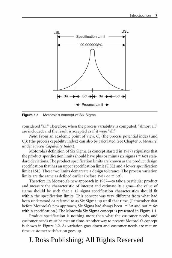
considered “all.” Therefore, when the process variability is computed, “almost all”are included, and the result is accepted as if it were “all.”
Note: From an academic point of view, Cp (the process potential index) andCpk (the process capability index) can also be calculated (see Chapter 3, Measure,under Process Capability Index).
Motorola’s definition of Six Sigma (a concept started in 1987) stipulates thatthe product specification limits should have plus or minus six sigma (� 6σ) stan-dard deviations. The product specification limits are known as the product designspecification that has an upper specification limit (USL) and a lower specificationlimit (LSL). These two limits demarcate a design tolerance. The process variationlimits are the same as defined earlier (before 1987 or � 3σ).
Therefore, in Motorola’s new approach in 1987—to take a particular productand measure the characteristic of interest and estimate its sigma—the value ofsigma should be such that a 12 sigma specification characteristics should fitwithin the specification limits. This concept was very different from what hadbeen understood or referred to as Six Sigma up until that time. (Remember thatbefore Motorola’s new approach, Six Sigma had always been � 3σ and not � 6σwithin specification.) The Motorola Six Sigma concept is presented in Figure 1.1.
Product specification is nothing more than what the customer needs, andcustomer needs must be met on time. Another way to present Motorola’s conceptis shown in Figure 1.2. As variation goes down and customer needs are met ontime, customer satisfaction goes up.
Introduction 7
3σ 3σ 3σ 3σ
Process Limit
Specification Limit
99.9999998%
LSL USL
Figure 1.1 Motorola’s concept of Six Sigma.
J. Ross Publishing; All Rights Reserved

Six Sigma is applicable to technical and nontechnical processes. A manufac-turing process is viewed as a technical process. There are numerous input vari-ables that affect the process, and the process produces transformation of inputs toan output. The flow of product is very visible and tangible. There are numerousopportunities to collect data. In many instances, variable data may be collected.
Nontechnical processes are more difficult to visualize. Nontechnical processesare identified as administrative, service, and transactional. Some inputs, outputs,and transactions may not be tangible. Yet, they are certainly processes. Treatingthem as systems allows them to be better understood and, eventually, to be char-acterized, optimized, and controlled, thereby eliminating the possibility for mis-takes and errors. Examples of nontechnical processes include:
• Administrative: budgeting
• Product/service selling: service
• Applying for school admission: transactional
Six Sigma is a highly disciplined process that helps organizations/businessesto focus on developing near-perfect products and services. It is a statistical termthat measures how far a given process deviates from perfection. The central ideabehind Six Sigma is that if the number of “defects” in a process can be measured,
8 Six Sigma Best Practices
CustomerNeeds
Bottom-Line Benefits to Business
Productsand
Services
Figure 1.2 The Six Sigma concept: customer needs vs. products and services.
J. Ross Publishing; All Rights Reserved

it is possible to systematically figure out how to eliminate them to get as close to“zero defects” as possible. Key concepts of Six Sigma include:
• Critical to Quality—The attribute most important to meet customerneeds
• Process Capability—What the process can deliver
• Defects, Errors, and Mistakes—Failure to deliver what customer wants
• Variation—What the customer perceives related to expectations
• Stable Operation—Maintains a consistent and predictable process toimprove throughput that the customer perceives related to expectations
• Design for Six Sigma—A Six Sigma program that allows the organiza-tion/business to meet customer needs and process capability
As an example, assume that a business manufactures 2-inch-thick, 3-ringbinders. The manufacturing cost of a binder is $3.00, which is inclusive of allcosts, including equipment, supplies, and production and supportive labor. Saythat if production yields at the 2.5 sigma (2.5 s) level, the business would reject(or produces in relation to defined specifications) 158,000 of 1,000,000 bindersproduced due to defects. The higher the sigma level, the better the performance.If the business were moved to the Six Sigma level, only 3.4 defective binders wouldbe rejected per 1,000,000 productions. Visualize what that would mean to theprofit margin.
Six Sigma, the Metric—The Six Sigma concept is also used as a metric for aparticular quality level. As an example, assume that a high sigma level may relateto a three sigma process, implying plus or minus three sigma (� 3σ) within spec-ifications. The quality level might be considered good, compared to a two sigmaprocess (� 2σ), in which there may be a plus or minus two sigma within specifi-cations, and in which the quality level is not so good. Therefore, the higher thenumber of sigma values within product/service specifications, the better the qual-ity level.
Six Sigma, the Strategy—Six Sigma can also be used in developing a businessstrategy for a product/service. For example, a product strategy could be based onthe interrelationship that exists between product design, manufacturing, delivery,product lead time, inventories, rework/scrap, mistakes in different processesthrough to delivery, and the level to which they impact customer satisfaction. Thevalue of Six Sigma is written statistically as follows:
� 6σ = 12σ
Introduction 9
J. Ross Publishing; All Rights Reserved

Six Sigma, the Management Philosophy—Due to global competition, SixSigma is also a customer-based approach, realizing that defects/errors/ mistakesare expensive and result in lower revenue and profit margin. Fewer defects meanlower costs and improved customer satisfaction and loyalty. Therefore, the lowest-cost and highest-value producer is the most competitive provider of products andservices. Six Sigma is a method to accomplish strategic business results.
With an understanding of Six Sigma, the next question might be “Who needsSix Sigma?” Consider two business situations:
• A business is performing poorly.
• A business is performing very well.
If a business is performing poorly, it might be experiencing some or all of thefollowing issues:
• Poor product quality
• Losing market share
• Competition gaining market share
• Business operating very inefficiently
• Poor service; customers complaining
Using the above-described situation, think how Six Sigma can help.
Six Sigma can be applied to the product design process, making the productmore robust, with improved manufacturability, which may result in better qual-ity and reliability to meet customer needs. Six Sigma can help the business tounderstand the science of its process. It can also help to reveal the variables thatsignificantly affect the process and the variables that do not.
Once identified, variables affecting the process can be manipulated in a con-trolled fashion to improve the process. When variables that truly influence theprocess are known with a high level of confidence, it is possible to optimize theprocess by knowing what inputs to control to maintain the process at optimumoutput performance.
If the business is performing very well, it may be selling more products/serv-ices than before and therefore needs more employees and a greater capacity todeliver more products/services in the same time frame to meet growing customerdemand. Six Sigma is more important for this business than for the businessdoing poorly. The successful business has more to lose than the one doing poorly.If the business is doing well, it must strive to excel through improvements andinnovations to become the standard by which others benchmark themselves.
10 Six Sigma Best Practices
J. Ross Publishing; All Rights Reserved

So far, “What is Six Sigma?” and “Who needs Six Sigma?” have been answered.The next logical question could be “What are the indications that Six Sigma isneeded?”
If a business is experiencing some of the following, then it needs to imple-ment the Six Sigma program:
• Customers complaining about product/service quality or reliability
• Losing market share
• High warranty cost
• Unpaid invoices due to customer complaints
• Wrong parts from suppliers
• Unreliable forecasts
• Actual cost frequently over budget
• Recurring problems, with the same fixes made repeatedly
• Design products very difficult to manufacture
• Frequency of scrap/rework too high and uncontrollable
Once any business leadership decides to implement the Six Sigma concept,leadership must understand the relationship between the sigma value and defectsin products/services. The numerical concept of Six Sigma is now introduced.
Numerical Concept of Six Sigma—Any process operating at � 6 sigma isalmost defect-free and therefore is considered to be “best in class.” In pure statis-tical terms, � 6 sigma means 0.002 defect per million parts, or 2 defects per bil-lion, or a yield of 99.9999998%. Motorola modified the pure statistical concept
Introduction 11
Table 1.1. Six Sigma Interpretation of Product/Service Quality
Product/ServiceAcceptable Range Sigma Yield (%) DPMOa
1σ 31.0 690,000
2σ 69.2 308,000
3σ 93.3 66,800
4σ 99.4 6,210
5σ 99.97 230
6σ 99.99966 3.4
aDPMO, defective per 1 million opportunities.
J. Ross Publishing; All Rights Reserved

(known as Motorola’s Six Sigma values). Some of these values are presented inTable 1.1. The bottom-line impact of Six Sigma is to reduce defects, errors, andmistakes to zero defects. The process will yield customer satisfaction, and happycustomers usually tell their friends about how pleased they are with a product orservice.
Because Six Sigma philosophy strives to produce a significant change in theprocess/product, a major barrier to Six Sigma quality is behavioral issues, not tech-nical issues. Fundamental rules for any significant change include:
• Always include affected individuals in both planning and implement-ing improvements.
• Provide sufficient time for employees to change.
• Confine improvements to only those changes essential to remove theidentified root cause(s).
• Respect an individual’s perceptions by listening and responding tohis/her concerns.
• Ensure leadership participation in the program.
• Provide timely feedback to affected individuals.
Therefore, Six Sigma is a quality improvement process with emphasis on:
• Reducing defects to less than 4 per 1 million
• Having aggressive goals of reducing cycle time (e.g., 40 to 70%)
• Producing dramatic cost reduction
According to Michael Hammer1 of Hammer & Co., Six Sigma is a powerfultool for solving certain kinds of business problems, yet it has severe limitations.For example, Six Sigma assumes that an existing process design is fundamentallysound and only needs minor adjustments. To be fully effective, Six Sigma shouldbe paired with other techniques that create a new process design that dramaticallyboosts performance. Process reengineering knowledge should show the user howSix Sigma should be positioned relative to other performance improvement tech-niques.
There may be situations in which a process reengineering2 application may berequired before implementing the Six Sigma concept. The concept of processreengineering will now be briefly introduced. Details of this concept are presentedin Chapter 5 (Improve).
Process activities are classified into three groups:
• Value Added—The customer supports the activity and is willing topay for it.
12 Six Sigma Best Practices
J. Ross Publishing; All Rights Reserved

• Non-Value Added—The customer is not interested and is not willingto pay, but the manufacturer/supplier needs the activity to supportthe business.
• Waste—The activity does not support either the customer or themanufacturer/supplier and nobody wants to pay for it.
The best ways to improve the process are to:
Eliminate—Waste
Minimize—Non-value added
Reprocess—Value added
The next section briefly introduces the steps of the Six Sigma process.
1.5 ROAD MAP FOR THE SIX SIGMA PROCESS
This discussion will start with a simple product life cycle, in which a customeridentifies the need; the supplier designs, manufactures, and delivers the product;and the service organization supports the product. The process to produce theproduct to meet customer needs is a set of structural and logical activities thatfocuses on the customer, cultivates innovation, ensures product robustness andreliability, reduces product cost, and ultimately increases value for the end cus-tomer and business owner (shareholders). Product quality must meet or exceedcustomer expectations. The quality concept in Six Sigma can be divided into twophases:
• A Product Design Quality Level Program
• A Product Manufacturing, Sales, and Service Quality Level Program
Product Design QualityIn the Six Sigma concept, product design quality is identified as a DMADVprocess (also Design for Six Sigma, DFSS methodology), where:
Define—Define the project goals and customer (internal or external)deliverables.
Measure—Measure and determine customer needs and specifications.
Analyze—Analyze the process options to meet customer needs.
Design—Design (detailed) the process to meet customer needs.
Verify—Verify the design performance and ability to meet customerneeds.
Introduction 13
J. Ross Publishing; All Rights Reserved

The DMADV process (DFSS methodology) should be used when:
• A product or process is not in existence at a business and one needs tobe developed.
• The existing product or process has been optimized using either DMAIC(to be discussed later) or some other process and it still does not meetthe expected level of customer needs or Six Sigma level metrics.
A documented, well-understood, and useful new product developmentprocess is a prerequisite to a successful DMADV process. DMADV is an enhance-ment to new product development process, not a replacement. DMADV is a busi-ness process concentrating on improving profitability. If properly applied, itgenerates the correct product at the right time and at the right cost. DMADV is apowerful program management technique.
Six Sigma initiatives at the product design quality level are tremendously dif-ferent from initiatives at the product manufacturing, sales, and service quality lev-els. However, the DMADV process is beyond the scope of this book, and itsprocess details will not be presented here. The fundamental differences betweenDMADV and DMAIC are presented in Table 1.2.
Product Manufacturing, Sales, and Service Quality Level ProgramAny process beyond the scope of DMADV is a part of a program called DMAIC,pronounced (Duh-May-Ick), where:
Define—Define the project goals and customer (internal and external) deliv-erables. Define is the first step in any Six Sigma process of DMAIC and identifiesimportant factors, such as the selected project’s scope, expectations, resources,
14 Six Sigma Best Practices
Table 1.2. Differences between DMADV and DMAIC
DMADV DMAIC
Focuses on the design of the product Looks at the existing processes and and processes fixes problem(s)
Proactive process More reactive process
Dollar benefits more difficult to Dollar benefits quantified ratherquantify and tend to be much more quicklylong term; may take 6 months toa year after launch of the new product before business will obtainadequate accounting data on the impact
J. Ross Publishing; All Rights Reserved

schedule, and project approval. This Six Sigma process definition step specificallyidentifies what is part of the project and what is not and explains the scope of theproject. Many times the first passes at process documentation are at a generallevel. Generally, additional work is required to adequately understand and cor-rectly document the processes.
Measure—Measure the process and determine current performance. The SixSigma process requires quantifying and benchmarking the process using actualdata. Yet, a Six Sigma process is not simply collecting two data points and extrap-olating some extreme data values. At a minimum, consider the mean or averageperformance and some estimate of the dispersion or variation (calculating thestandard deviation is beneficial). Trends and cycles can also be very informative.Process capabilities can also be calculated once performance data are collected.
Analyze—Analyze the data and determine the root cause(s) of the defects.Once the project is understood and baseline performance is documented, estab-lishing the existence of an actual opportunity to improve performance, the SixSigma process can be utilized to perform a process analysis. In this step, the SixSigma process utilizes statistical tools to validate root causes of problems (issues).Any number of tools and tests can be used. The objective is to understand theprocess at a level that is sufficient to facilitate formulation of options (develop-ment of alternative processes) for improvement. A team should be able to com-pare the various options to determine the most promising alternative(s). It isalso critical to estimate financial and/or customer impact on potential improve-ment(s). Superficial analysis and understanding will lead to unproductive optionsbeing selected, forcing a recycle through the process to make improvements.
Improve—Improve the process by eliminating defects. During the Improvestep of the Six Sigma process, ideas and solutions are implemented. The Six Sigmateam should discover and validate all known root causes for the existing opportu-nity. The team should also identify solutions. It is rare to come up with ideas oropportunities that are so good that all of them are instant successes. As part of theSix Sigma process, checks must ensure that the desired results are being achieved.Sometimes, experiments and trials are required to find the best solution. Whenconducting trials and experiments, it is important that all team members under-stand that these are not simply trials, but that they are actually part of the SixSigma process.
Control—Control the implemented process for future performance. As a partof the Six Sigma process, performance-tracking mechanisms and measurementsmust be in place to ensure that the gains made in the project are not lost over aperiod of time. As a part of the control step, telling others in the business aboutthe process and the gains is encouraged. By using this approach, the Six Sigma
Introduction 15
J. Ross Publishing; All Rights Reserved

process starts to create potentially phenomenal returns: ideas and projects in onepart of the business are translated to implementation in another part of the busi-ness in a very rapid fashion.
The DMAIC process can also be presented as:
Define � Measure � Analyze � Improve � Control
These are the five key steps in the Six Sigma process. Every process goesthrough these five steps. The steps are then repeated as the process is refined.
Key guiding elements that team members should strive to avoid or minimizeas they go through the Six Sigma process include:
• Leadership resistance
• Unclear mission
• Limited dedicated time for the project
• Prematurely jumping to a solution
• Untrained team members
• Unsatisfactory implementation plan
To implement the Six Sigma program, business/organization members mustbe assigned defined responsibilities. These members must take their responsibili-ties seriously.
As a high-level organization structure is defined, the management groupshould also begin identifying Six Sigma projects. The implementation structureand project selection are parallel processes. The next two sections will discuss theSix Sigma implementation structure (identifies program participants and theirresponsibilities) and program selection (selecting a project that qualifies as a SixSigma project).
1.6 SIX SIGMA IMPLEMENTATION STRUCTUREImplementation of the Six Sigma program is very demanding. Simply explainingthe implementation of Six Sigma to employees and expecting them to implementthe program is an approach that is clearly not enough for a program such as SixSigma that has a demanding level of excellence. This type of approach would cre-ate numerous unanswered questions and have undefined directions for almost allemployees. Specifically, inexperienced employees would struggle, developing theirown version of what the Six Sigma program is or ought to be and how it shouldbe carried out. Generally, this type of approach would yield a very poor successrate and probably lower program acceptance and expectations. It could alsoshorten the program’s life. A practical strategy is required. It must include all nec-essary elements for a successful implementation of the Six Sigma program.
16 Six Sigma Best Practices
J. Ross Publishing; All Rights Reserved

Organization structure is one of the challenges in implementing the SixSigma program. In the last 10 to 15 years, major corporations such as Motorola,GE, and Xerox have implemented the program very successfully. Their organiza-tional structures had a critical role.
The Six Sigma ChallengeOnce executive leaders of a business have decided to implement the Six Sigmaprogram, they must challenge each employee in the business. Six Sigma involvesall employees.
Because the process is physical and tangible, and metrics are commonly uti-lized to judge the output quality in a manufacturing environment, it is easy (andobvious) for manufacturing employees to implement the program. (Remember:Administrative and service activities do not have similar metrics.)
Each employee in the business provides some kind of service. Therefore,employees must assess their job functions and/or responsibilities in relationshipto how the Six Sigma program will improve the business. Employees shoulddefine what would be their ideal service goals in support of customer (internaland external) needs and wants. Once their goals are established, employees shouldquantify where they currently are in relationship to these goals. Then they mustwork to minimize any gaps to achieve Six Sigma goals in accordance with targetdates.
Prerequisites for the implementation structure and the functional concept ofthe organization as presented in Figure 1.3 include:
• Businesses with profitable Six Sigma strategies are successful.
• Profitable businesses must maintain effective infrastructures.
• Profitable businesses are continually improving and revising throughexecutive planning.
• Businesses must be creative and customer-focused.
• Implementation of Six Sigma is a team process.
• Executive leadership and senior management must be part of theprocess.
• Six Sigma is not a quick-fix process. It requires a months-long tomulti-year commitment.
• Key participating leaders must be supported by an organizationalinfrastructure with key roles:
– Executive Leadership
– Steering Committee
– Champion
– Master/Expert/Project Team(s)
Introduction 17
J. Ross Publishing; All Rights Reserved

Chief Executive’s CommitmentOnce the business leader (Chief Executive) expresses his/her commitment to con-verting the business into a Six Sigma organization, he/she establishes the chal-lenges, vision, and goals to meet customer needs and wants. The new metrics andnew way of operating the business are also established. Old vs. new ways of doingbusiness are compared. New ways of working toward excellence and establishinga common goal for all employees in the business reduce variability in everyprocess they perform.
18 Six Sigma Best Practices
ExecutiveSponsorship
SteeringCommittee
Master/Champion
Experts/Project Teams
Expandsinvolvementto additionalassociates
Reports lessonslearned and
best practices
Motivates andsustains change
Control the keyprocess input
variables
Businessstrategy
Figure 1.3 The Six Sigma implementation structure.
J. Ross Publishing; All Rights Reserved
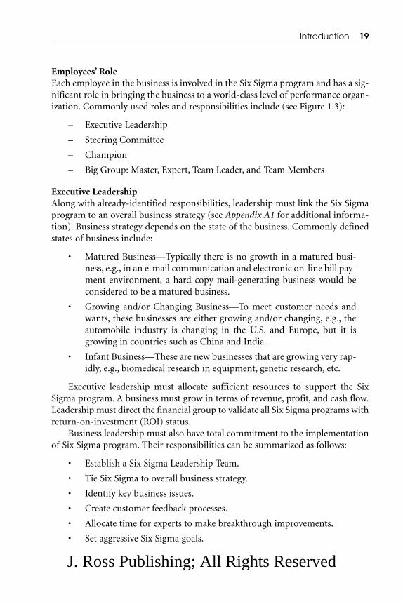
Employees’ RoleEach employee in the business is involved in the Six Sigma program and has a sig-nificant role in bringing the business to a world-class level of performance organ-ization. Commonly used roles and responsibilities include (see Figure 1.3):
– Executive Leadership
– Steering Committee
– Champion
– Big Group: Master, Expert, Team Leader, and Team Members
Executive Leadership Along with already-identified responsibilities, leadership must link the Six Sigmaprogram to an overall business strategy (see Appendix A1 for additional informa-tion). Business strategy depends on the state of the business. Commonly definedstates of business include:
• Matured Business—Typically there is no growth in a matured busi-ness, e.g., in an e-mail communication and electronic on-line bill pay-ment environment, a hard copy mail-generating business would beconsidered to be a matured business.
• Growing and/or Changing Business—To meet customer needs andwants, these businesses are either growing and/or changing, e.g., theautomobile industry is changing in the U.S. and Europe, but it isgrowing in countries such as China and India.
• Infant Business—These are new businesses that are growing very rap-idly, e.g., biomedical research in equipment, genetic research, etc.
Executive leadership must allocate sufficient resources to support the SixSigma program. A business must grow in terms of revenue, profit, and cash flow.Leadership must direct the financial group to validate all Six Sigma programs withreturn-on-investment (ROI) status.
Business leadership must also have total commitment to the implementationof Six Sigma program. Their responsibilities can be summarized as follows:
• Establish a Six Sigma Leadership Team.
• Tie Six Sigma to overall business strategy.
• Identify key business issues.
• Create customer feedback processes.
• Allocate time for experts to make breakthrough improvements.
• Set aggressive Six Sigma goals.
Introduction 19
J. Ross Publishing; All Rights Reserved

• Allocate sufficient resources.
• Incorporate Six Sigma performance into the reward system.
• Direct finance to validate ROI for all Six Sigma projects.
• Evaluate the corporate culture to determine if intellectual capital isbeing infused into the company.
• Expand involvement to additional associates.
Steering CommitteeThe Steering Committee is a high-level group of managers (executives) whoreports program status and achievements to the business CEO in relationship tooverall business strategy. The Steering Committee must continuously evaluate theSix Sigma implementation and development process and make necessary change,as well as:
• Define a set of cross-functional strategic metrics to drive projects.
• Create an overall training plan.
• Define project selection process and criteria.
• Supply project report-out templates and structured report-out dates.
• Evaluate diversity issues and facilitate change.
• Provide the appropriate universal communication tools wherebyindividuals must feel that there is something for everyone.
• Collect lessons learned and share best practices.
ChampionsChampions are managers at different levels in the business. They define the stud-ies and/or projects. Projects are either improvement or characterization studies.Project savings could vary from several thousand dollars (U.S.) to as much as amillion dollars. Savings depend on business size, project scope and duration, andproject activities. A Champion’s function is to inform the steering committee andkeep track of the project team’s progress. Champions also provide high manage-ment visibility, commitment, and support to empower team members for success.They provide strategic directions for the projects and ensure that changes,improvements, or solutions are implemented. They must motivate experts andsustain change. Champions officially announce the project team and the projectcompletion after all project objectives are met and the documentation is com-pleted. They also organize the team’s presentation to senior management.Champions are also responsible for:
20 Six Sigma Best Practices
J. Ross Publishing; All Rights Reserved

• Selecting at least one project in each standard business unit that willhave the most benefits.
• Selecting the experts from the cross-functional team members.
• Identifying the appropriate project leaders among the experts.
• Monitoring team progress and help remove barriers.
• Converting gains into dollars.
Big Group: Master, Expert, Team Leader and Team Members Responsibilities of this large group can be divided into subgroups: Master andExpert, Team Leader, and Team Members
Master—A Master (also Master Black Belt) is generally a program-site tech-nical expert in Six Sigma methodology and is responsible for providing technicalguidance to team leaders and members. Often a Master is dedicated to support theprogram full time. A Master is considered to be an expert resource for the teams:for coaching, statistical analysis, and Just-In-Time (JIT) training. A Master, alongwith team leaders, determines team charter, goals, and team members; formalizesstudies and projects; and provides management leadership. A Master can supportup to ten projects.
Expert, Team Leader, and Team Members—These resources are a criticalpart of studies and projects:
Expert. Generally, an Expert is not a full-time member of the team. An Expertis invited to participate when there is a need for explanation, advice, technicalinput, etc. An Expert trains and coaches team members on tools and analysis. AnExpert also helps the team if there is any misunderstanding or incomplete under-standing of the process.
Team Leader. A Team Leader (at the least a Black/Green Belt-trained person)is responsible for implementing the team’s recommended solution to achieve thedefined goals of the Six Sigma project. He/she is an active member of the team andalso is in charge of the overall coordination of team activities and progress. ATeam Leader is responsible for assigning responsibilities to all team members,tracking the project goals and plans, managing the team’s schedule, and handlingadministrative responsibilities. Improvement projects must demonstrate substan-tial dollar savings and significant reduction in variation, defects, errors, and mis-takes. The Team Leader position is not necessarily a full-time team assignmentunless the project requires a full-time Team Leader or if the Team Leader is lead-ing two or three projects.
Introduction 21
J. Ross Publishing; All Rights Reserved

Team Members. Team Members are employees who maintain their regularjobs, but are assigned to one or more teams based on their knowledge and expe-rience in selected Six Sigma projects. They have full responsibility as TeamMembers in the project. Team Members are expected to carry out all assignmentsbetween meetings, devote time and efforts toward the team success, conductresearch as needed, and investigate alternatives as necessary.
Common responsibilities of Master, Expert, Team Leader, and TeamMembers include:
• Measure the process.
• Analyze/determine key process input variables.
• Improve the process as they recognize and make changes as necessary.
• Control the key process input variables.
• Develop the Expert’s network to enhance communication.
• Convert gains into dollars.
• Use the Six Sigma DMAIC process to solve problems and/or improveprocess.
If Master, Expert, and Team Members were compared, a few distinctive qual-ities would be found (see Table 1.3). A conceptual flow chart is presented in Figure1.3.
As indicated earlier, the Six Sigma Implementation Structure and the ProjectSelection are almost parallel processes.
1.7 PROJECT SELECTION
All businesses face problems that are solved on a daily basis by employees as a partof their normal jobs. Routine, daily problems should not become Six Sigma proj-ects. If a business is functioning well, there is probably no need for a Six Sigmaproject, but if employees are trapped in a constant cycle of reacting to problemsinstead of fixing the root causes, then ways that Six Sigma could help might needto be explored. A list of issues that indicate signs of existing problem may befound in an earlier section (The Six Sigma Approach). If any of these issues arefound in the following situations, then the issue or problem has become a candi-date for a Six Sigma project:
• The business has tried to fix the process several times (three to four)with no success.
• The business has tried to fix the process, and the problem stoppedoccurring, but it has recurred.
22 Six Sigma Best Practices
J. Ross Publishing; All Rights Reserved

Considerations include:
• Project Choice—Management should be careful to choose projectsthat are large enough to be significant, but not so large as to beunwieldy.
• Business Case—What are the compelling business reasons for select-ing this project? Is the project linked to key business goals and objec-tives? What key business process output measure(s) will the projectleverage and how? What are the estimated cost savings/opportunitieson this project?
Six Sigma program is highly mathematical. Its basis is the application of sta-tistics in engineering for the reduction of variability and for meeting customerneeds. Therefore, to understand project selection for a Six Sigma project, theexplanation must be a bit technical.
Generally any product selected as a Six Sigma project will have numerouscharacteristics. Consider a very simple product such as a lid for a glass bottle. Alid has at least five characteristics: diameter, depth, threads, material, and paint. Amore complex product such as power chain saw could have as many as 300 char-acteristics. An even more technically complex product such as riding lawn mowercould have several thousand characteristics. Finding a product with a single char-acteristic is impossible.
Yet, a product with only one characteristic will be used for our purposes ofdiscussion. Assume that the quality level or performance in producing this char-acteristic follows the “old concept” of specification limits of � 3 sigma (� 3σ). Itcan be inferred that about 99.73% of the product would be good and about 0.27%would be defective by failing for that characteristic. The product yield of such aprocess would be 99.73%. This result is referred to as a three sigma product (� 3σ).
Introduction 23
Table 1.3. Profile Comparison of Master, Expert, and Team Member
Master Expert Team Member
Manager, experienced Technically oriented, Highly visible in companyemployee, respected respected by peers and trained in Six Sigmaleader and mentor and managementof business issues
Strong proponent of Master of basics Respected leaders andSix Sigma; asks and advanced tools mentors for expertsthe right questions
J. Ross Publishing; All Rights Reserved

Historically, a process that was capable of producing 99.73% product withinspecifications was considered to be very efficient. In such a process, only 0.27%product would nonconform to specifications and might be rejected. If 10,000units of that product were produced, 9,973 units would be good and 27 unitswould be defective. Now, if 1 million units of that product were produced,997,300 units would be good and 2,700 units would be defective and most likelywould be reworked.
These situations do not seem to be too bad, but, unfortunately, not even thesimplest of products has only one characteristic. Now consider a product that hasmore than 1 characteristic, e.g., a power chain saw for which 300 characteristicshave been identified. Imagine that product quality is defined based on perform-ance of only four characteristics at a plus or minus three sigma levels (� 3σ). Thisimplies that each of the four characteristics has a fraction nondefective of 0.9973and a fraction defective of 0.0027. If these characteristics were independent, thenthe yield would be 98.92% (0.9973 � 0.9973 � 0.9973 � 0.9973 = 0.9892).
This result also does not appear to be of great concern, but if all 300 charac-teristics were performing at a three sigma (� 3σ) level, each with a quality of0.9973 fraction nondefective, then the yield for the power chain saw would be44.437%, i.e., yield = 100 � (0.9973)300 = 44.43%. Therefore, for every 100 powerchain saws, only 44 would go through the entire production process without a sin-gle defect and about 56 of them would have at least 1 defect. If this manufacturerhas received an order for 1 million power chain saws, and 1 million power chainsaws were produced, then only 444,371 would be defect-free and the other555,629 would have at least 1 defect per power chain saw.
The example clearly demonstrates that to be competitive in the marketplaceand to build a product with zero defects, the first time, with no scrap, the qualityat the characteristic level has to be much better than 99.73% or three sigma (� 3σ).
To produce power chain saws with zero defects, no scrap, and no rework thefirst time around, the manufacturer has to increase the performance capability atthe characteristic level to Six Sigma—or 99.9999998% nondefective. If every char-acteristic in the power chain saw was performing at Six Sigma, then the first-passyield would be 99.99994% or 100 � (0.999999998)300.
In the power chain saw example, if all 300 characteristics are at Six Sigma, andthe manufacturer has produced 10,000 power chain saws, all would be defect-free.If the manufacturer were to produce 1 million power chain saws, only 1 mighthave defects or be defective and the other 999,999 would be defect-free. Underthese conditions:
• There would be no need to have a rework line.
• There would be no cost for rework, personnel, and equipment.
24 Six Sigma Best Practices
J. Ross Publishing; All Rights Reserved
• There would be minimal to no scrap.
• There would be a significant reduction in product cycle time.
• Predictability of on-time delivery would be realized.
Clearly, achieving all the product/service characteristics at a Six Sigma levelmakes the process defect-free, cost-effective, and potentially very profitable. Thepower chain saw example provides a prospective for project selection. It is a two-step process:
• Identification of Quality Costs and Losses
• The Project Selection Process
1.7.1 Identification of Quality Costs and LossesWhen choosing Six Sigma projects, not overlooking the cost-savings potential ofsolving less-obvious problem issues is important. Traditionally, costs related topoor quality are identified by:
• Rejects
• Scrap
• Rework
• Warranty
Other issues that impact quality and increase product/service costs must notbe excluded from Six Sigma projects:
• Engineering change orders
• Long cycle time (order booking and manufacturing)
• Time value of money
• More setups
• Expediting costs
• Allocations of working capital
• Excessive material orders/planning
• Excess inventory
• Late delivery
• Lost customer loyalty
• Lost sales
Introduction 25
J. Ross Publishing; All Rights Reserved
1.7.2 The Project Selection ProcessOne of the most difficult activities in Six Sigma deployment is the project selec-tion process. Projects can be divided into two types based on project savings: hard(bottom-line) savings and soft savings. Hard savings data can be obtained from afinancial analysis of year-to-year spending, budget variance, and improvements inrevenue. Hard savings could be a result of cost reduction, revenue enhancement,or a combination of both. Examples are presented in Table 1.4. Soft savings, on theother hand, are difficult to quantify, but soft savings may result in lowering capi-tal and/or budget requirements. Examples are presented in Table 1.4. Additionalexamples are on-time delivery, customer satisfaction, improvement of the sys-tem’s process potential index (Cp), and improvement of the system’s process capa-bility index (Cpk). Cp and Cpk are discussed in Chapter 3, Measure.
Additional elements impact selection of the right project:
• Correct selection of a right project can have a tremendous effect onthe business. Once the project is implemented, processes will functionmore efficiently, employees will feel satisfied, and ultimately, share-holders will see the benefits.
• If a right project selection is made incorrectly and the selected projectdoes not have full business buy-in, project roadblocks may not beremoved due to other business priorities, the project team may feelineffective, and the end result may be less than ideal. No one winsunder these situations. Select a right project that is in line with busi-ness priorities.
• Ask business leaders, “What are the three greatest issues facing thebusiness?” Ensure that the project chosen addresses one of these issuesor is directly related to one of them. Including an important issue willincrease the probability that the management team provides theproper attention and quickly removes hurdles to ensure successfulcompletion of the project.
• Ask a similar question to customers.“As a customer, what are the threegreatest issues at our company that are of concern to you?” To sup-port customer issues, investigate data from sources such as customercomplaints. Specifically call customers who have cancelled servicesfrom the business.
• A selected project should be completed within 6 months. If theselected project is of longer duration, the team leader may lose teammembers as they take on other projects or other jobs.
26 Six Sigma Best Practices
J. Ross Publishing; All Rights Reserved
Information presented so far provides a broad view of project selection, sav-ings, and sources. The following are more formalized steps for the project selec-tion process that will lead to the project’s mission statement:
1. Identify potential problems.
2. Obtain information/data.
3. Prioritize problems.
4. Characterize problems.
5. Evaluate and select project.
6. Prepare mission statement.
Discussing the six steps is facilitated by using an example. The setting is a jetengine manufacturing company. Assume that the company has a Six Sigma teamleader. He is an employee in the jet engine manufacturing company. He has askedthe company’s business leaders a question: “What are the three greatest issues fac-ing the business?” Responses from the business leaders would likely include:
• Losing revenue
• High inventory
• High resources cost
The following discussion will utilize the six steps to identify potential prob-lem(s) for the jet engine manufacturing company.
Step 1: Identify Potential ProblemsThe Six Sigma team leader wants to identify the potential problem(s) that resultin loss of revenue. Revenue is derived from customers when they purchase jetengines. The Sales group sells the engines and the Service group provides servicefor the engines after they are sold. Generally, the Sales and Service groups are thelast groups that maintain contact with customers.
As previously discussed, sales and services are processes just like any otherprocess such as product designing and manufacturing. A process can be presentedas a set of inputs, which, when used together, generates a corresponding set ofoutputs. Therefore, “a process is a process,” regardless of the type of organizationand the function of the process. All processes have inputs and outputs. Allprocesses have customers and suppliers. All processes may exhibit some level ofvariation. The Six Sigma team has to understand the root cause(s) of the varia-tion, find alternative solutions, and select and implement the best possible alter-native to minimize/eliminate the variance. To identify a potential problem(s), theteam leader needs to analyze the inputs, the process, and the outputs with the keyelements as listed below. This process is known as IPO (Input-Process-Output):
Introduction 27
J. Ross Publishing; All Rights Reserved

Inputs:
• Cost of unacceptable quality
• Unsatisfied customer
• Business strategy and plans
• Reviews and analysis of input data
• Management and other employees
Process:• List potential problems as identified by each source and their impact on:
– Maintaining existing customers
– Attracting new customers
– Return on investment
– Reducing the cost of unacceptable quality
– Improving employee satisfaction
• Investigate key information sources in the organization.
Outputs:
• Evaluate process inputs.
• Develop a detailed list of potential Six Sigma projects.
• Input information into project evaluation.
Note: Output from an IPO process becomes input for a project evaluationprocess, in which it is compared with customer needs. IPO output must meet cus-tomer needs.
It is critical to understand the IPO process and relate how inputs are linked tooutputs. The IPO process is used to develop a list of potential Six Sigma projects.(Remember: Six Sigma applies to manufacturing and nonmanufacturingprocesses.) Because revenue lost is a sales process, an IPO diagram for a salesprocess has been developed (Figure 1.4). The next step is to investigate and obtainprime sources of information managed by the manufacturer (the jet engine com-pany) and by customers.
Step 2: Obtain Information/Data Several sources of information can help uncover issues affecting revenue:
• Customers—Customer opinions are important. Customer com-plaints can provide clues to problems that need to be addressed.
28 Six Sigma Best Practices
J. Ross Publishing; All Rights Reserved

Introduction 29
Table 1.4. Examples of Hard and Soft Savings
Savings Type: Revenue improvement
Savings Category: Hard savings
Definition: Increased throughput over the planned level to meet market demandwithout any major capital expenditure. Additional savings will be a product of anincrease in throughput and the product’s profit margin.
Example: A Six Sigma project was implemented in the inserter manufacturing area.The project improved throughput by 16% above the planned baseline.
Savings Type: Cost reduction
Savings Category: Hard savings
Definition: Decrease in spending from prior year’s baseline budget. These savingscan be normalized for changes in production.
Example: The Six Sigma project improved the efficiency of the heating system in thecustomer service building, resulting in a 15% savings in heating gas year after year.
Savings Type: Cash flow improvement
Savings Category: Soft savings
Definition: Reduction of capital tied up in inventory/components, WIP, and finishedproducts.
Example: A Six Sigma supply chain project was implemented, resulting in 25–50%reduction in suppliers’ lead time. Therefore, inventory was reduced.
Savings Type: Capital avoidance
Savings Category: Soft savings
Definition: Eliminated or deferred future capital. This was an approved capitalfunding either for the current year or for a future year.
Example: The Six Sigma project improved the grinding process, resulting ineliminating the need for an additional set of grinders.
Savings Type: Cost avoidance
Savings Category: Soft savings
Definition: Eliminated or deferred future expenses. These expenses have notoccurred and they were not budgeted.
Example: A test machine was consuming more-than-normal material to perform atest. A Six Sigma project was implemented to reduce material consumption at thetest machine. The Six Sigma project brought material requirements to normal levels.
J. Ross Publishing; All Rights Reserved

• Product Reviews/Audits—Many manufacturers maintain data on thecost of poor quality in the areas of Quality Assurance, Internal Audit,and Management Engineering.
• Business Plans—Businesses develop strategic plans with goals andother business objectives. Some of these plans may call for significantquality improvement projects.
• Managers/Other Company Employees—Managers and other associ-ates are often the first to recognize opportunities to improve the prod-uct and customer service.
As information is obtained from the sources helps to identify problems, col-lect specific objective data on each problem or process that has been identified asa potential project. Collected/available data should answer some of the followingquestions:
• What complaints and dissatisfaction issues are most likely to driveaway existing or new customers? Example: Commercial jet engine cus-tomers are typically airlines. Airlines cannot afford to keep a jet planeon the ground because a few jet engine parts are needed from the jetengine manufacturer.
30 Six Sigma Best Practices
SalesProcess
Sales Volume
Number of Defects
Number of Contract Errors
Number of Lost Sales
Number of Sales-RelatedCustomer Complaints
Input Process Output
Product Line Intelligence
Customer Relationship
Sales SOP
Pricing Policy
Sales Workforce
Sales Training
Sales Incentive System
Competitor Intelligence
Product Distribution
Sales Follow-Up Policy
Payment Policy
Contract CompletionCycle Time
Profit Margin
Sales Person Uniformity
Sales Identification ofCustomer Needs
Market Share
Figure 1.4 Input-Process-Output (IPO) diagram for sales process.
J. Ross Publishing; All Rights Reserved
• What are our most costly deficiencies? Example: The jet engine man-ufacturer’s difference (deficiency) in original cost estimation for over-haul of a jet engine vs. the final billing. Generally, original estimatesare too low compared to the final cost of overhauling a jet engine.
• What level of performance does the competition deliver and how doesit compare with our level of performance?
• Which deficiencies in our internal processes have the most adverseaffect on employees?
Brainstorming. Sometimes brainstorming can be used to develop a list ofpotential problems. Brainstorming is an excellent approach to generate a list ofideas, but it must not be a substitute for information or data collection. Theremust be no judgment or analysis of ideas during a brainstorming session. One ora few individuals should not dominate the presentation of ideas.
In brainstorming, it is critical to recognize that the differences between cre-ativity and logical thought do not imply that there are differences in the truth orusefulness of ideas produced. It is the method by which an idea is produced that isthe difference. Logical thought follows rules and can be reproduced by anyoneusing the same rules. Creative thought is not determined by rules and usually can-not be duplicated by others. Key steps in a brainstorming process include:
1. Preparation for the Session—The purpose statement must focus onthe issue. The statement must be broad enough to allow creativity,but have no leading emphasis. Communicating the purpose of thesession ahead of time is very helpful for participants. An ideal num-ber of participants would be six to ten.
2. Introducing the Session—Describe and review basic brainstormingrules:
– Ideas will be listed on a flip chart or a visible screen.
– No criticism or evaluation of any type will be permitted.
– Use unconventional thinking.
– Aim for many quality ideas in a short time.
– Using another person’s idea as a basis for one’s own idea will beallowed and acceptable.
– Make contributions in turn.
– Contribute only one idea per turn.
– A participant may pass.
– Do not provide an explanation of ideas.
Introduction 31
J. Ross Publishing; All Rights Reserved

3. Warming Up—Sometimes it is helpful to conduct a warm-up ses-sion with a neutral topic for 5 to 10 minutes.
4. The Session—Explain the issue. Write the issue so that it will be vis-ible to all participants. End the session before participants showfatigue. A session can last for 20 to 40 minutes.
5. Processing Ideas—Once the brainstorming session is over, continueworking with the team to:
– Clarify each idea
– Combine and group similar ideas
– Collect data on ideas wherever available
– Proceed with a cause-and-effect diagram for the ideas that haveno data
By this time, the problems that have been identified must be in list form.Working on all problems on the list may not be possible. Therefore, the problemsmust be prioritized.
Step 3: Prioritize the ProblemsOnce a list of problems is developed, the next step is to select a problem from thedeveloped list. Key elements must be kept in mind when evaluating problems forselection:
• What are the costs and paybacks?
• How much time is needed to find a solution and implement the solution?
• Probability of success in developing and implementing a solutionboth technologically and organizationally?
• What processes are you responsible for?
• Who is the owner of these processes?
• Who are the team members?
• How well does the team work together?
• Which processes have the highest priority for improvement?
• How was this conclusion reached? Do data support this conclusion?
The nominal group technique (NGT) is a structured process that identifiesand ranks major problems or issues that need addressing. The NGT is used for:
• Identifying the major strengths of an institution/unit/department andmaking decisions by consensus when selecting the problem solution
32 Six Sigma Best Practices
J. Ross Publishing; All Rights Reserved

• Providing each participant with an equal voice (e.g., defusing a dom-inating sales team member or influential employee who tends to con-trol the discussion and dominate the process)
Steps to follow when conducting the NGT include:
1. Request that all participants (usually five to ten people) write orstate the problem/issue that they perceive is most important.
2. Develop a master list of the problems/issues (e.g., losing revenue ina jet engine business).
3. Generate and distribute to each participant a form that numbers inno particular order the problems/issues. Request that each partici-pant rank the top five problems/issues by assigning five points to theproblem they perceive to be most important and one point to theleast important of their top five.
4. Tally the results by adding the points assigned to each problem/issue.The problem/issue with the highest score will be the most importantproblem for the total team.
5. Discuss the results and generate a final ranked list for action plan-ning.
The NGT application is presented in Example 1.1. This process will berepeated for each issue. Finally, there will be a proposed solution for each issue.The business may not have enough resources to solve all of the issues at the sametime. Therefore, the issues with their proposed solutions must be prioritizedagain. As problem solutions are selected through NGT, these problems should becharacterized according to customer needs and business strategy before going onto the next round to prioritize the selected solutions for the issues.
Note: The goal of every business is to completely satisfy customers and also toimprove profit margin. Customer satisfaction is derived by meeting customerneeds; the profit margin is linked to business strategy.
Example 1.1: An NGT Application
Five possible solutions to a problem have been identified. There are six teammembers who must decide which solution should be attempted first. Thesolutions are identified as I, II, III, IV, and V. The team members are identified asA, B, C, D, E, and F.
Each member of the six-person team orders the potential solutions, produc-ing the following matrix:
Introduction 33
J. Ross Publishing; All Rights Reserved

Solution A B C D E F Total
I 1 2 1 4 3 5 16II 5 5 2 5 5 4 26III 4 3 3 3 1 2 16IV 2 1 4 1 2 1 11V 3 4 5 2 4 3 21
Based on the matrix, solution II should get the highest priority followed bysolution V.
Step 4: Characterize the ProblemsAlthough each of the following questions might not apply to the solution of everyissue, the following questions are commonly asked. They help to identify theneeded information as well as to sort the information:
• How is the process performed?
• What are the process performance measures and why?
• How accurate and precise is the measurement system?
• What are the customer-driven specifications for all of the perform-ance measures?
• How good or bad is the current performance?
• What are the improvement goals for the process?
• What are all the sources of variability in the process?
• Which sources of variability do you control? How do you controlthem and how is it documented?
• Are there any sources of variability that are supplier-dependent? If so,what are they, which supplier(s) is responsible, and what is being doneabout it?
• What are the sensitive (key) variables that affect the average and thevariation of the measures of performance? Support the characteristicswith data.
• What are the relationships between the measures of performance andthe key variables? Do any variables interact? Support/validate thecharacteristic with data.
Once the listed questions have been answered, enough identified and sortedinformation exists to move on to Step 5, which is to evaluate and select a solutionfor the issue. This becomes the Six Sigma project for the team.
34 Six Sigma Best Practices
J. Ross Publishing; All Rights Reserved

Note: Because data from the jet engine manufacturing company are confiden-tial, information about the issue of “losing revenue” is not presented here.
Step 5: Evaluate and SelectThe elements of this step are summarized in the IPO process with the nominalgroup technique (NGT), where:
Input is a list of top-priority projects (with decision-making data).
Process is to evaluate the top-priority projects utilizing NGT, with the follow-ing as some of the key criteria:
• Continuing problem
• Significant improvement in product/service
• Measurable improvement
• Support the business strategy
• High probability of success
• Customer satisfaction
• Support resistance
• Project risk
Output is to select a Six Sigma project. Once the project is selected, preparingthe mission statement is next.
Step 6: Prepare Mission StatementManagement should review the mission statement following Step 6 of the projectselection process. The defined mission statement should describe the problem thatthe project team has to resolve. The IPO process can be used to prepare the mis-sion statement, where:
Input identifies the problem/issue (e.g., losing revenue)
Process describes the problem/issue and identifies the project team’sobjectives to resolve the problem.
Output develops a mission statement to resolve or minimize the problem.
The following criteria apply to the problem description and the mission state-ment. An effective problem description and a mission statement must be:
• Specific—Explain exactly what is incorrect; do not include other busi-ness problems. Similarly, state what is to be accomplished in the mis-sion statement.
Introduction 35
J. Ross Publishing; All Rights Reserved
• Measurable—The scope of the problem must be quantifiable. Be pre-pared to answer questions such as “How many?” “How often?” “Howmuch?” (Also be prepared to state the case for the mission statement.)
• Observable—Project team members and/or others should be able toactually observe the problem (also the case for the mission statementonce the proposed solution is implemented).
• Manageable—The problem can be resolved in a clearly defined time.
A mission statement:
• Must consider business objectives and strive to understand what thebusiness wants to accomplish.
• Must indicate the objective of the project, i.e., what the project teammust do to solve the problem.
An effective problem description and a mission statement must exclude:
• Blame—Assigning blame. Do not assign blame to any individualand/or group. Assigning blame may create defensive behavior andinterfere with the team’s ability to collect and analyze data objectively.
• Cause—Identifying a cause. Identifying a cause(s) in the missionstatement may prevent discovery of the true cause(s) of the problem.
• Remedy—Suggesting a solution. Do not suggest/propose a solution. Asuggested solution might be incorrect. Product/service quality maybecome worse than expected.
Therefore, problem statement for the jet engine manufacturing companymight be: “The Company is losing revenue of $200 million a year, which is 1% ofthe world’s commercial market.”
A flow chart of the process described in this section is presented in Figure 1.5and Examples 1.2 and 1.3. Analyze the team’s mission statement from the perspec-tive of what must be included and what must be excluded from a mission state-ment. Different views of the objective are presented in Example 1.4. Once theproject’s problem description and mission statement are prepared, the next step isto select the project team.
Example 1.2: Write an Effective Problem Statement
“Our construction company’s house foundation construction project takes 8 dayslonger on average than our major competitors take.”
36 Six Sigma Best Practices
J. Ross Publishing; All Rights Reserved
The problem statement must have four key characteristics: specific, measura-ble, sbservable, and manageable. These four key characteristics are also appropri-ate for the mission statement. The following is the statement analysis:
• Specific—The statement names a specific process and identifies theproblem.
• Measurable—House foundation construction time is measured indays.
• Observable—Evidence of the problem can be obtained from internalreports and customer feedback. The process can be physicallyobserved.
• Manageable—The problem is limited to one type of construction pro-cedure, which can easily be managed.
Example 1.3: Analyze Ineffective Issues in the Problem Statement
Avoid suggesting who is to blame, the cause, and a remedy in the mission state-ment and the problem statement, e.g.:
• Assigning Blame: “Our construction company’s house foundationconstruction project takes 8 days longer on average than our majorcompetitors take. The foundation design department needs toimprove their work procedures to reduce the time needed to con-struct the house foundation.”
Comment: This problem statement implies that the foundation designdepartment is to blame for the problem. If any project team memberis from the foundation design group, he/she would manifest a defen-sive behavior, which could hurt the team’s ability to collect and ana-lyze data objectively.
• Implying a Cause: “Our construction company’s house foundationconstruction project takes 8 days longer on average than our majorcompetitors take. We should improve the communication processbetween the foundation designers and the concrete company.”
Comment: Implies that the communication process between the foun-dation designers and the concrete company needs to be improved.After collecting and analyzing data, communication between thefoundation designers and the concrete company might not be themain cause of the problem.
• Suggesting a Remedy: “Our construction company’s house foundationconstruction project takes 8 days longer on average than our major
Introduction 37
J. Ross Publishing; All Rights Reserved

38 Six Sigma Best Practices
Step 1: Identify Potential Problem(s) Sample Business – Jet Engine Manufacturing CompanyPotential Problems
• Losing Revenue • High Inventory• High Resources Cost
Selected Problem – Losing Revenue Process IPO – Applied to Sales ProcessAnalyzed – Inputs, Process, and Outputs
Step 2: Obtain Information/Data Obtained information directly or through the following sources:
– Customer– Product Review/Audit– Business Plans– Managers and/or other employees– Another source could be used
Brainstorming session – Follow the procedure; will provide a list of problems that might be creating the selected issue (losing revenue)
Step 3: Prioritize the Problem Utilize Nominal Group Technique to prioritize the identified problems.
Step 4: Characterize the Problem A list of problem characteristics is provided. Answer as many characteristic questions as applicable.
Step 5: Evaluate and Select Even though the problems have been prioritized using NGT, at this step, evaluate the prioritized problems in relation to problem characteristics and select one that could be used to write the mission statement.
Step 6: Prepare Mission Statement
Figure 1.5 Process flow chart of project selection.
J. Ross Publishing; All Rights Reserved

competitors take. Install a designers’ log on the company web page tospeed up the communication process.”
Comment: Without knowing the cause of the problem, finding aneffective solution to the problem is impossible.
Exercise 1.2: Evaluate Problem Descriptions
Read each problem statement. Decide if a statement is effective or ineffective.Rewrite any ineffective statement.
1. Our on-time delivery of systems is low.
2. Our service department on an average receives 20 complaint tele-phone calls per week about unsatisfactory service.
3. Communication between our departments at this facility is poor.
4. More than 40% of our customers responded in a mid-year surveythat they were very or somewhat dissatisfied with our serviceresponse time.
Example 1.4: Presenting Different Objective Views from a ProblemStatement
Problem: Too many software programs must be modified to support the installa-tion of a message printing and packaging system. On average, 30% of all programsmust be modified at least once, which causes missed project completion (due)dates and expenditures that are above the budgeted amount.
Objective 1: Reduce the number of program modifications.Comment: There is a high probability that Objective 1 could be met by increasingthe allocated program design time, but that would not guarantee that programswould not require modification by the program team and that project due dateswould not be missed.
Objective 2: Reduce the number of project run-over days from defined due date.Comment: Objective 2 might focus on scheduling an additional programmingresource or overtime hours to complete the installation by due date.
Objective 3: Reduce the installation margin so that the actual cost of installationwill not exceed budget.Comment: Objective 3 focuses on completing the installation project withinbudget estimates.
Choosing between the three objectives will be determined by the concern thatis of most importance to the business: customers complain about installation due
Introduction 39
J. Ross Publishing; All Rights Reserved

dates being missed; the cost incurred is high, and the installation due date is beingmissed; or program modification is required when the installation design isdefective.
Exercise 1.3: Evaluate Mission Statements
Mission statements include problem and objective descriptions. Read these mis-sion statements and provide an opinion about whether the statements are effec-tive or ineffective. If a statement is ineffective, indicate how it could be improved.
1. Reception (guest checkout desk) at Hotel X does not inform theHousekeeping group quickly when a guest checks out of the hotel.Objective: Improve communications between Reception andHousekeeping to reduce the time needed for room cleaning/prepa-ration.
2. Shipping Department takes too long to ship spare parts to dealers.Objective: Reduce the time it takes for parts to reach dealers.
3. We need a project scheduling and tracking website to plan a project’sactivities, to target milestone dates, and to track the actual comple-tion of planning activities.Objective: Procure and install e-project management system by theend of the fiscal year.
4. Credit Corporation C experienced interest loss of $1 million lastyear due to billing errors and the resulting late credit card payments.Objective: Minimize the interest loss resulting from card billingerrors.
1.8 PROJECT TEAM SELECTION
Team members chosen to work on solving a problem should be the most quali-fied individuals in the company. Showing appreciation of differences in teammembers is the key to acknowledging the value of each team member.Differences are the “raw material” for healthy discussions among the team mem-bers. The team selection process should follow these steps:
• Business areas that are the most closely connected to the problemshould be identified. Ask:
– Problem location—Where is the problem observed?
– Problem source—Where could sources or causes of the problembe found?
40 Six Sigma Best Practices
J. Ross Publishing; All Rights Reserved
– Problem root cause and solution—Who has knowledge, under-standing of the problem, or capabilities to uncover the rootcause(s) of the problem?
– Group to implement problem solution—What group in the busi-ness organization would be helpful in implementing a solution?
• Team members should represent the required business areas.
• Each team member should have direct and detailed personal knowl-edge of some part of the problem.
• Time required for meetings and time required for team-related workbetween meetings should not be during the team members’ sparetime.
• Team members should be able to accurately describe the processesassociated with the problem and the interconnecting links associatedto the problem elements.
Members selected for the project team should have as many of the followingqualities as possible:
• Participates based on agreed upon goals/objectives
• Listens and analyzes all brainstorming ideas
• Has clear objectives
• Accepts differences
• Engages in healthy conflict
• Not dominating
• Trusts others in group
• Supports team decision process
• Shares information with team members
• Clearly perceives roles and work assignments (Expectations about therole of each team member should be clearly defined. When action istaken, assignments are clearly made and are accepted and carried out.Work should be fairly distributed among the team members.)
Once the project team has been identified, the team leader must develop theproject plan and start thinking about how to manage the project from implemen-tation to final documentation.
Introduction 41
J. Ross Publishing; All Rights Reserved

1.9 PROJECT PLANNING AND MANAGEMENT
Project planning starts once the project has been identified. The first step in theprocess is project justification and approval. Generally, the assigned project leaderdevelops a document known as the Project Proposal for project justification andapproval. Once the project is approved, the project leader’s responsibility is toachieve the project objectives within budget and on time. This process is knownas Project Management.
1.9.1 Project ProposalA business determines how the project proposal form is developed. A sample for-mat is presented in Figure 1.6. A project proposal generally begins with identifi-cation of the project:
Project: ___________________________ Project #: ___________________________
Key sections in the proposal should include:
Problem Statement: Describe the problem/opportunity that is forcing the busi-ness to develop the proposal. Answer important questions such as:
• What is the problem?
• Under what conditions does the problem occur?
• What are the extent and the impact of the problem?
Example: “In the past 2 years, 150 cases of customer complaints have occurred inthe U.S. market: 65 of 100 printing through message packaging systems wereinstalled that were more than 10 days after customers’ requested dates. Customercomplaints and ad hoc attempts to resolve installation issues caused loss of pro-ductivity (i.e., wasted time and productivity), internal conflict among staff, andloss of potential revenues and repeated business.”
Objective Statement: State what is expected to be accomplished in specific, meas-urable, observable, and manageable terms once the project is completed, based ona given budget and time duration.
Example: “To reduce from 65 to 25 of 100 installations of printing through mes-sage packaging systems taking more than 10 days from the customer-requesteddate by improving the process capability from 1.1 sigma to 2.2 sigma in the next6 months. This will provide a 2.7 times improvement in the process.”
42 Six Sigma Best Practices
J. Ross Publishing; All Rights Reserved

Expected Benefits: Identify the importance of the project and its relationship tothe company’s business strategy. State the financial benefits that are expected andhow these benefits will be achieved.
Example: “Targeted savings: DPMO reduction (defects per million opportunities):
• Reduction of system installation delays (from 65 to 25 of 100 systeminstallations that are completed beyond 10 days of the customer-requested date).
Introduction 43
Project: Project #:
Problem Statement:Objective Statement:Expected Benefits:
Project Scope:Project Criteria:Project Plan:Project Team and Expertise:
General Information:Business Strategy:Critical Quality Issue:Current Process Capability:Comments (Remarks):
Project Review Dates (Dates to Complete Each Phase)Start Date: Define Date:Measure Date: Analyze Date:Improve Date: Control Date:Closure Date:
Approval Signatures:Functional Manager Champion
__________________ ______ _________________ ______ DateDate
Experts Team Leader
__________________ ______ _________________ ______ DateDate
Other Other
__________________ _______ __________________ _______ Date Date
Figure 1.6 Sample project approval form.
J. Ross Publishing; All Rights Reserved

The team would expect total financial benefits of $100,000 before taxes in the next12 months and an additional cost savings of $20,000. The qualitative benefitswould be reduction in staff conflicts, reduced customer complaints, and improvedcustomer satisfaction.”
Project Scope: Specifically identify what is included and what is excluded in thescope of this project.
Example: “The project team will focus on the process from order bookingthrough system installation: starts once the customer signs the contract and endswhen the system installation is complete. Customer credit check and paymentdays are excluded from the process.”
Project Criteria: State the relationship of this project to other projects as applica-ble. If this project is a part of a program (a program is made up of several proj-ects), identify and link to the program. Specify if ROI is required or if any specificperson/group is to approve the activity/output.
Example: “Message printing through packaging system’s pricing policy will beupdated based on the results (output) of this project.”
Project Plan: Identify key activities that would lead to the project objectives.
• Develop material and process flow charts.
• Collect routing and volume data.
• Collect material lead time.
• Develop area layout with assumed constraints.
• Develop hardware and software integration milestone activities.
Project Team and Expertise: State the responsibilities of individuals/groups.
• Management team
• Project leader and his/her team—Core team members who have thestrongest interest in the process improvement (These individuals areinvolved in day-to-day work on the project and devote a significantamount of their time to the project.)
• Core team members—Subject matter experts who will be called uponfrom time to time if specialized knowledge is required for the project
Note: Team leaders must define their responsibilities and provide a realisticexpectation of the time commitment required.
44 Six Sigma Best Practices
J. Ross Publishing; All Rights Reserved

General Information: Any general information about the business strategy, crit-ical quality issues, current process capability, and comments (remarks). Reviewdates and approval signatures are also key areas in a project proposal.
Financial Benefits: Give special attention to financial benefits. Financial benefitsshould be estimated based on the business case language, which should comedirectly from the owner. If the business owners are not identified, the team willneed to draft its own rationale. Financial benefits may change as the project pro-gresses from one stage to the next. Therefore, the following are critical to estimatefinancial benefits:
• Financial benefits should be estimated at the beginning of the project.They should be linked to business strategy.
• Financial benefits should be based on the project definition, bestavailable data, assumptions, and auditable benefits. They should beadjusted as the project progresses through the different phases of theDMAIC process and reaches implementation stage.
• As process performance is measured against the baseline, any incre-mental improvement will be measured and recognized.
• As the project goes through the Analyze phase, the team determinesthe root causes of the problem and assesses the assumptions used inestimating the benefits. Financial estimates should be revised toincorporate the new data.
• As the best solution is selected to improve the process, a completecost/benefit analysis should be done to incorporate the cost of imple-menting the selected solution and should be adjusted the bottom-linebenefits of the improvement (projected benefits).
• As the project is implemented, measure and report the actual benefits.
Note: It is important to list all the assumptions made at the different stages ofthe project.
1.9.2 Project ManagementProject management can be described in simple terms:
• Project management is the business of securing the end objectives inthe face of all risks and problems that are encountered from beginningto end of the project.
• Project success depends largely on carrying out the constituent tasksin a sensible sequence and deploying resources to best advantage.
Introduction 45
J. Ross Publishing; All Rights Reserved

Project Leader: As a minimum, the project charter must provide that the ProjectLeader will:
• Be accountable for accomplishing the project objective with the avail-able or anticipated resources and within the constraints of time, cost,and performance/technology.
• Clearly define the “deliverables” to be given to the sponsor (cham-pion) at the end of the project.
• Maintain prime customer liaison and contact.
• Be responsible for establishing the project organization and providean effective orientation for the project staff at the beginning of theproject.
• Provide for a well-balanced workload for the project team.
• Ensure that the best performers are assigned to work on the “criticalpath” activities of the project.
• Develop and maintain project plans (who does what, for how much,and when).
• Negotiate and contract with all functional disciplines to accomplishthe necessary work packages within time, cost, and performance/technology.
• Provide technical, financial, and schedule requirements direction.
• Analyze and report project performance.
• Define and communicate security and safety requirements for theproject as appropriate.
• Serve as an effective conductor in coordinating all-important aspectsof the project.
• Get problems “out in the open” with all persons involved so that prob-lems can be resolved.
• Make a special effort to give recognition to each staff member forhis/her individual accomplishments.
• Maintain a current milestone chart that displays planned milestonesand actual achievement of milestones.
• Review the technical performance of the project on a continual basis.
• Prepare a formal agreement if there is any scope change agreed to withthe sponsor (champion).
46 Six Sigma Best Practices
J. Ross Publishing; All Rights Reserved

Project Activities: A project activities flow chart is presented in Figure 1.7.
Project Success: Potential challenges to the project’s success include:
• Sponsor (Champion) is not actively involved.
• Project objectives are not clearly and precisely defined.
• Results metrics is not clearly defined.
• Project team is large (ideal size is 8 ± 2).
• Team members do not have enough time to support the project.
• Project does not support the business strategy.
• Very difficult to obtain the required data.
• Team members do not have proper training.
Exercise 1.4: Project Activity
Develop project approval information to cover the first three sections of the sam-ple form presented in Figure 1.6.
Introduction 47
SponsorRequirements
Define
Measure
Analyze
Improve
Control
Redefining Reporting
Figure 1.7 Project activities flow chart.
J. Ross Publishing; All Rights Reserved

1.10 PROJECT CHARTER
Generally, a project charter is a one-page report, presenting business informationabout the project. A project charter is the easiest way to communicate informa-tion about the project to others in the company. It includes the following, but it isnot limited to only to these items:
• Business Case—Briefly states how the project is related to the business(organization)
• Goal Statement—Primarily contains the mission statement withexpected benefits
• Project Plan/Time Line—Provides the project schedule with some keymilestone activities and sigma metrics (if possible) (The projectschedule should include at least the time line for the different phasesof the DMAIC process.)
• Opportunity Statement—Presents statements about the project thatwill provide qualitative and quantitative benefits to the business
• Scope—Identifies the key issue areas
• Team Members—Identifies full-time and part-time participatingteam members
A sample project charter is presented in Figure 1.8.
1.11 SUMMARY
Overview information presented in this chapter includes:
• Recent past history of quality leading to the birth of the Six Sigmaconcept
• Discussion of how the business market has changed and its expectations
• Statistical meaning of sigma
• Qualitative and quantitative meaning of Six Sigma
• Organizational commitments and responsibilities in a Six Sigma program
• Quality and business loss relationship
• Road map for Six Sigma process (a brief definition of each step in theprocess)
• Impact of Six Sigma program on organizational structure
• IPO analysis approach
• Problem ranking procedure
• Problem characteristics
48 Six Sigma Best Practices
J. Ross Publishing; All Rights Reserved

Introduction 49
Project CharterManufacturing Cycle Time Reduction for Product XYZ
Business Case: Because the customer is expecting a quality product with on-time delivery at a competitive price, the company must produce the product with increased quality and reduced cycle time and business cost. This project will reduce manufacturing cycle time.
Goal Statement: Reduce the manufacturing cycle time• For product XYZ1 from 45 calendar days to 30 calendar days,
33% cycle time reduction by Month Year• For product XYZ2 from 95 calendar days to 70 calendar days,
26% cycle time reduction by Month Year
• Improve the inventory turns from 4 to 4.5 per year by Month Year • Reduce inventory (Raw, WIP, and Finished) from $XX millions to $YY
millions by Month Year to provide $(XX – YY) freed-up capital
Project Plan/Timeline: Based on Year XXXX objectives, Six Sigma goal metrics projections:
Six Sigma MetricProduct Jul XX Oct XX Dec XX
XYZ1 1.4 1.6 1.8XYZ2 1.7 1.9 2.1
Opportunity Statement: Reducing the manufacturing cycle time will:• Speed product delivery• Reduce inventory• Reduce manufacturing cost• Improve customer satisfaction
Scope: Reduce the manufacturing cycle time of products XYZ1 and XYZ2 by resolving/minimizing the following issues:• Product stability• Engineering support on the manufacturing floor• On-time delivery of quality material on the manufacturing floor• Process reengineering the manufacturing activities
Team Members: John Smith – Black Belt (Team Leader); Dave Moore – Champion; Thomas Murphy – Master Black Belt; Robert Lynch – Green Belt: Ram Dosi – Green Belt; Carol Perez – Financial Support; Brad Potter – Expert
Figure 1.8 Sample of project charter (names of team members are hypothetical).
J. Ross Publishing; All Rights Reserved

• Description of problem and development of mission statement
• Project team selection process
• Project proposal development
• Project leader’s responsibilities
• Potential challenges to project success
• Project charter
The program implementation structure has been defined, the project missionhas been stated, the project team has been selected, and the team has defined howto plan and manage the project. Think about answers to the following questionsbefore moving on to the discussion in Chapter 2 (Define):
• Has the project team charter been defined clearly, including businesscase, problem and mission statement, project scope, milestones, rolesand responsibilities, and communication plan?
• Who are the improvement project team members, including ProjectLeader/Black Belts, Master Black Belts/Coaches, Team Members, andExperts?
• Has each member of the team, including the Team Leader, been prop-erly trained in DMAIC?
• Will the team meet regularly?
• Do the team members regularly have 100% attendance at team meet-ings? If any team member is absent and appoints a substitute to attendthe meeting, does the substitute preserve cross-functionality and fullrepresentation?
• Has the project work been fairly and/or equitably divided and dele-gated among team members who are qualified and capable of per-forming work? Is each member of the team contributing?
• Are there any known constraints that would limit the project work?How is the team addressing them?
• How is the team tracking and documenting their work?
• Has the team been adequately staffed with the required cross-func-tionality? If not, what additional resources are available to the team tominimize the gap?
REFERENCES
1. http:/www.hammerandco.com/PowerOfProcessFrames/PowerOfFrames9.html.
50 Six Sigma Best Practices
J. Ross Publishing; All Rights Reserved

2. Hammer, M. 1996. Beyond Reengineering, Harper Collins Publishers,New York, 1996, Part I (Work) and Part II (Management).
ADDITIONAL READING
Dean, J.W., Jr. and J.R. Evans. 1994. Total Quality, West Publishing, St.Paul, MN, Chapter 1.
Introduction 51
This book has free material available for download from theWeb Added Value™ resource center at www.jrosspub.com
J. Ross Publishing; All Rights Reserved

J. Ross Publishing; All Rights Reserved

53
2
DEFINE
Define means to establish the cause of a problem and to set the boundaries of theproblem. The Define phase helps the team to picture the process over time andprovides insight for the team about where the focus of improvement effortsshould be (e.g., on improving the door seal on a frost-free refrigerator). Definealso applies to customers, customer needs, and customer requirements (known ascritical to quality characteristics or CTQs) and to the core business processesinvolved.
CTQs are the key measurable performance characteristics of any product,process, or service that satisfy external (ultimate) customers. CTQs must be met.
In the Define phase, it is critical define who the customers are, what theirrequirements for products and services are, and what their expectations are. It is
Define
Measure
Analyze
Improve
Control
6σ DMAIC
J. Ross Publishing; All Rights Reserved

also important to define the project’s boundaries—where to start and where tostop the process. Additionally, there must be definitions of the process and whatthe team must improve. Process understanding can be obtained by mappingprocess flow. Sections include:
2.1 The Customer2.2 The High-Level Process2.3 Detailed Process Mapping2.4 SummaryReferencesAdditional Reading
2.1 THE CUSTOMER
The traditional definition of a customer is “someone who buys what the supplier(company) sells,” but in today’s global competitive market, the traditional defini-tion is neither a precise nor a complete definition. A better definition is “a cus-tomer is a person who a company/supplier tries to understand (e.g., theirreactions and expectations) and to provide with products/services that meet thecustomer’s needs.” This much broader definition is far more useful in today’sincreasingly complex business environment with its wide variety of customers. Acustomer does not see or care about a company’s organizational structure or itsmanagement philosophies. A customer only sees the products and experiences theservices offered by that company.
A company/customer relationship can be very complex. In the following list,who is a customer of a pharmaceutical company?
• The patient, who uses the medicine
• The pharmacist, who dispenses the medicine
• The physician, who prescribes the medicine
• The wholesaler/distributor, who is an intermediary between the man-ufacturer and the pharmacy
• The Food and Drug Administration scientists and officials, whoapprove the use of medicine
• An insurance company that pays indirectly for the medicine
The answer is all in the list are customers. Therefore, a pharmaceutical com-pany must understand the requirements (needs) of all of these individuals andinstitutions.
Another type of company is one that produces consumer goods. This com-pany has at least two types of customers: individuals who purchase and use the
54 Six Sigma Best Practices
J. Ross Publishing; All Rights Reserved

company’s products and retailers. A customer goods company can influence thesecustomers in two ways:
• The company wants retailers to carry its products, to allocate substan-tial shelf space to them, and to promote the products in advertisingpieces.
• The company wants to influence customers to select and use in itsproducts.
This presents a very complex company/customer relationship. The funda-mental relationship between a company and its customers is not based on theexchange of products or services for money. It is actually based on providing val-ued products/services that meet customer needs in a timely manner and at com-petitive prices.
“What is a business?” If contemporary managers, executives, and economistswere asked this question, most likely they would answer, “The mission of a busi-ness is to create shareholder value.” This answer is neither irrational nor unrea-sonable, but nonetheless it is “wrong.” Why?
Because shareholders provide capital that produces an income stream, share-holder concern must be central to an enterprise. Yet, exclusive focus on capital andthose who provide it can be a distraction in a company from what really counts.Fundamentally, every company is in the same business—the business of “identi-fying and meeting customer needs.” Customers define product/service needs thata manufacturer/supplier delivers. Customers can be divided into three groups:internal, external, and stakeholders.
Note: Unfortunately, shareholder concern was not a primary concern duringthe 1960s and the 1970s. Many executives ran their companies as if the companieswere their personal businesses. These executives followed business strategies thatmainly boosted their egos and personal incomes. Many received a nasty surprisein the takeover wave of the 1980s.
Internal Customers. Internal customers are a part of the total process if theyreceive internal/external output and utilize it as an input in their process to sup-port their customers. These customers may be another internal customer or theexternal ultimate customer (the ultimate user of a product/service).
External Customers. External customers are not only product/service users,but also governmental agencies (e.g., regulators and law enforcement agencies)and the public (or community). An external customer could be domestic or for-eign. Most business revenue is generated from external customers, making themthe most important customers.
Define 55
J. Ross Publishing; All Rights Reserved

Stakeholders. Stakeholders sponsor the project. Periodically, the project teamreports project status to stakeholders. Stakeholders impact the process or theprocess impacts them.
Customers and Critical to Quality CharacteristicsIf a company is working on something that is aligned to its strategic business pri-orities, then any improvements made for an internal customer will ultimately leadto a quantitative improvement for external customers. The product/service per-formance characteristics must also satisfy customers. Additionally, a suppliermust understand the needs of customers. Customer-needs information can becollected by surveys, e-surveys, focus groups, etc. Information collected must betranslated into comments, issues, and specifications. These comments, issues, andspecifications then become customer CTQs. A CTQ is a product or a service char-acteristic that must be met to satisfy a specification or a requirement(s) of a cus-tomer (i.e., the recipient of a final or an end product/service, generally an externalcustomer). A CTQ may also be referred to as project Y [as in Y = f(X)]. The fol-lowing example relates CTQs to customers.
Suppose that your company produces software packages for sale to customers(external). To define design specifications and develop the software, you mustunderstand the CTQs of the customers. You also must understand time-to-mar-ket, total software development cost, and on-time delivery of quality software (interms of defects) to meet customers’ needs. Customers (internal and external) canbe identified as:
• Purchasers/users of the software
• Stakeholders imposing requirements on the software:
– Shareholders
– Regulators
– Government agencies
• Users of internal software
– Business partners
Once identified, customers can have different requirements that must be con-sidered in determining CTQs. Therefore, to ensure that the “proper” requirementshave been considered when collecting customer data, all possible customer andstakeholder groups must be identified. Internal stakeholders often speak for exter-nal stakeholders (customers); their process requirements must be met if the busi-ness is to be successful. Key internal stakeholder groups and their requirementscould include:
• Financial—Internal Revenue Service (IRS), Securities and ExchangeCommission (SEC)
56 Six Sigma Best Practices
J. Ross Publishing; All Rights Reserved

• Legal—Regulatory agencies
• Compliance—Government agencies
• Human Resources—Occupational Safety and Health Administration(OSHA), Equal Employment Opportunity (EEO)
Therefore, the term “needs” (requirements) must consider stakeholdergroups and customer segments to accurately determine CTQs.
CTQs Defining ProcessDefining customer CTQs is a three-step process:1 identify, research, and translate(Figure 2.1). The process delivers:
• Prioritized list of internal and external customers and stakeholders
• Prioritized customer needs
• CTQs to support needs
Identify: Customer—As presented in Figure 2.1, and with the types of cus-tomers identified with examples in the previous section, the next step in theprocess is to prioritize the customers. The highest priority goes to the external(ultimate) customer, prioritized as:
1. External customer (ultimate customer)
2. Individual/groups that have direct or indirect responsibility for theproduct, service, or process:
– Business shareholders
– Internal/external regulators
– Government agencies
3. Internal/external service groups and material suppliers:
– Business partners
Listening to customers and collecting pertinent data that reflect their inputare important. Internal customers often develop solutions for the ultimate cus-tomer and their requirements. Internal customer departments could include:
• Business development
• Financial
Define 57
Identify � Research � Translate
Figure 2.1 Steps of a CTQ Defining Process
J. Ross Publishing; All Rights Reserved

• Personnel
• Legal
• Safety and security
Example 2.1: A CTQ Process—House Construction Proposal
The process is a house construction proposal from a general contractor to anexternal customer (ultimate customer). An architect will develop a house designpackage for a general contractor (internal customer). The package will include ahouse design, drawings, and construction cost estimates. The general contractorwill prepare the final document for an external (ultimate) customer.
Identify Internal and External Customers:
Internal Customer(s)
•
•
•
•
External Customer(s)
•
•
•
•
Identify CTQs:
Sample CTQs: House Design Quotation
• House design to meet customer requirements
• House layout to meet space requirements
• House construction to meet budget and schedule requirements
•
•
•
•
Once customers have been identified, the next step is to research the cus-tomers.
58 Six Sigma Best Practices
J. Ross Publishing; All Rights Reserved

Research Customer—Before beginning this step, first determine how well youunderstand and listen to your customers. Do you have little or no information ordo you have detailed information? Are you confident about the quality of yourcustomer information? If data are historical, answer the following:
• What do you know about the data?
• What is your level of certainty that your customer data represent theopinions/needs of the majority of your specified customers and/orgroups?
• Are your data reliable and representative of all your customers?
A natural progression of this step is that you might start with no information,but conclude with quantified, prioritized customer needs and expectations, aswell as information about your competitor.
The three elements of a Research Customer process (Figure 2.2) include:
• Collect data.
• Analyze data.
• Prioritize data.
A basic guideline for Research Customer is presented in Table 2.1.
Note: A detailed discussion of data collection may be found in the DataCollection Plan and Data Presentation Plan sections of Chapter 3 (Measure).
Collect data. Based on the available information, determine if additionalinformation is needed, e.g., to fill “data gaps.” Then develop a data collection planto close the gap(s) between “where you are” and “where you need to be.” Data canbe collected in several ways, e.g., sampling methods include:
• Listen to sales representative, service representative, and customercomplaints and to customer compliments.
• Analyze product returns.
• Perform a direct contact survey.
• Analyze contract cancellations.
• Survey, e.g., with direct mail questionnaires and e-questionnaires(website).
• Analyze customer defections.
• Interview new customers.
• Interview focus groups.
Define 59
J. Ross Publishing; All Rights Reserved

Analyze data. As data are collected, a high level of data analysis will indicate:
• If any additional information is needed
• If complaint data indicates the cause of dissatisfaction (which couldfacilitate collecting the additional needed data)
Sometimes the initial analysis reveals that additional information still isneeded.
This high-level data analysis will identify customer requirements and help theteam to develop a detailed plan to validate and translate “the voice” of the cus-tomer. As data are collected and analyzed, understanding the following is critical:
• What percent of the customer base is covered by data collection?
• What level of customer needs will be satisfied by the selected priorities?
• How reliable are the data?
• How is information collected, analyzed, and prioritized?
60 Six Sigma Best Practices
Identify Research Translate
Customer Needs
Collect Analyze Prioritize
Sampling Methods– Listen
Sales representative Service representativeCustomer complaints
– Interviews– Surveys– Websites
Sampling Methods– Level of qualitative
information– Quantitative
information– Need for any
additional information– Develop hypothesis
and test throughdata analysis
Sampling Methods– Interviews– Surveys– Websites
Figure 2.2. Research Customer Analysis
J. Ross Publishing; All Rights Reserved

• What competitor information has been collected?
• What level of “gap” analysis is performed prior to collecting any data?
Collected data may be either qualitative or quantitative or a combination ofboth. Collected data could also be defined as independent or dependent variables.To establish a relationship between dependent and independent data, the projectteam may have to develop a hypothesis and then test it. The hypothesis concept isdiscussed in Chapter 4 (Analyze).
Prioritize data. Customer needs should be translated into product/servicefunctionalities, which can be classified into five categories:
Define 61
Table 2.1. Selecting the Appropriate Research Methods
Input: No information (data)
Research Method: Analyze information requirements.Interview individual/focus groups.Listen to customer complaints.
Output: What you get: Customer needs and wants providing general ideas;combination of qualitative and quantitativeinformation; unprioritized
Input: If preliminary customer needs and wants are known
Research Method: Interview individual/focus groups.Analyze underlying needs and develop specificquestions.
Output: What you get: Customer needs and wants — Clarified; morespecific; prioritizedCustomer input to list — Best in class; may be acompetitor
Input: Qualitative; prioritized customer needs and wants
Research Method: Survey — Face to face; regular mail; electronic mail;telephoneQuestions based on most important requirements
Output: What you get: Quantified and prioritized customer needs and wantsMay get competitor’s comparative information
J. Ross Publishing; All Rights Reserved
• Expected—Satisfaction derived from expected functionalities isdirectly proportional to the availability of these functionalities in theproduct/service, i.e., when they are fully functional.
• Required—Some customers have a specific requirement of function-alities. If required functionalities are not up to the required level, cus-tomers become dissatisfied. Yet, if the required functionalities wereabove the customer’s required level, customer satisfaction would notincrease, e.g., a mainframe computer’s required up-time is 99%; dur-ing the last 5 days, up-time was 99.5%, but the customer/user satis-faction level did not increase.
• Optional—The customer is more satisfied if optional functionalitiesare added to the product/service, but the customer is not less satisfiedin the absence of them, e.g., a five-speed standard transmission in anautomobile instead of a four-speed standard transmission.
• Indifferent—If advanced functionalities were provided in aproduct/service, only a small fraction of customers would be inter-ested in using these functionalities. These functionalities generally donot change customer satisfaction values, e.g., Microsoft® Office witha special feature such as Excel Solver.
• Reserve—Sometimes reserve functionalities cause dissatisfaction,particularly if they negatively impact the customer’s plans or activi-ties. Customer satisfaction then decreases, e.g., some vacation resortsprovide computer games, but the parents prefer that their childrenengage in personal interaction.
Once the customer’s information is prioritized, going back to the customer tovalidate the assigned priorities is critical. Communication with a customer mightinclude interviews, surveys, and a website.
The Research Customer process is presented in Figure 2.2. In summary, at aminimum, Research Customer is a three-step process. If time permits, use addi-tional steps to achieve a better understanding of customer “needs and wants:”
• Selecting the right tool to collect customer information is very impor-tant. If no customer “needs and wants” information is available, talkto or interview focus groups and evaluate: “What is important?” and“What are customer needs and wants?”
• After obtaining the preliminary customer “needs and wants” informa-tion, interview additional customers from different geographic loca-tions to help develop specific requirements. Then prioritize the “needsand wants” requirements.
62 Six Sigma Best Practices
J. Ross Publishing; All Rights Reserved

• Survey customers. Commonly used methods include:
– Face to face – e-mail
– Electronic – Mail
– Telephone
Quantify the survey results and then try to analyze the competitor’s information.The conceptual relationship between customer satisfaction and product/serv-
ice is presented in Figure 2.3. This concept is based on Kano’s theory. The linepassing through the origin at 45 degrees represents the situation in which cus-tomer satisfaction is directly proportional to the functionality of theproduct/service, meaning the product/service functionality is meeting customerneeds. The customer is more satisfied with a more fully functional product/serv-ice (per customer needs) and is less satisfied with a lesser functioningproduct/service. According to Kano’s definition, such requirements are known as“one-dimensional” requirements.
In Figure 2.3, if the customer satisfaction and product/service relationshipresides in the first quadrant, the product/service will be unacceptable to cus-tomers and the business will not survive. If the product/service is functional anda good percentage of customer needs are being met, then the product/service andcustomer satisfaction relationship will fall in the second quadrant. However, toproduce a fully functional product/service, a business must implement a contin-uous improvement program. A continuous improvement program will move theproduct/service and customer satisfaction meeting point into the third quadrantas shown by the dashed arrow. Yet, if the product/service is functional, but cus-tomer satisfaction is low, then the product/service and customer satisfaction rela-tionship will fall in the fourth quadrant. This situation indicates the business is ona critical path for survival: the combination of customer satisfaction and prod-uct/service would need to follow the dashed-line arrow in the fourth quadrant.
Using an automobile as an example, priorities in a competitive marketinclude:
• Automobile reliability and safety
• Driver and passenger comfort
If the automobile (the product) meets these requirements, it would be in thethird quadrant. If the automobile is reliable and safe, but the driver and passen-gers are uncomfortable, the automobile will fall into the second quadrant. It isnow on a critical path. For the business to survive, significant effort will berequired by the business to make the automobile fully functional and to fully sat-isfy customers.
In a scenario in which the driver and passengers in the automobile are com-fortable, but the automobile has reliability and safety ratings that are low, the rela-
Define 63
J. Ross Publishing; All Rights Reserved
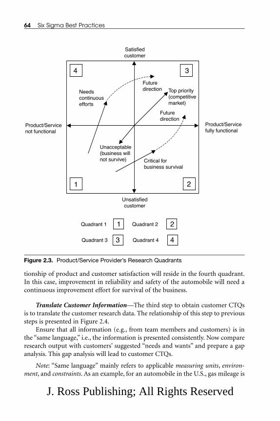
tionship of product and customer satisfaction will reside in the fourth quadrant.In this case, improvement in reliability and safety of the automobile will need acontinuous improvement effort for survival of the business.
Translate Customer Information—The third step to obtain customer CTQsis to translate the customer research data. The relationship of this step to previoussteps is presented in Figure 2.4.
Ensure that all information (e.g., from team members and customers) is inthe “same language,” i.e., the information is presented consistently. Now compareresearch output with customers’ suggested “needs and wants” and prepare a gapanalysis. This gap analysis will lead to customer CTQs.
Note: “Same language” mainly refers to applicable measuring units, environ-ment, and constraints. As an example, for an automobile in the U.S., gas mileage is
64 Six Sigma Best Practices
Product/Servicefully functional
Product/Servicenot functional
Satisfiedcustomer
Unsatisfiedcustomer
Top priority(competitivemarket)
Unacceptable(business willnot survive) Critical for
business survival
Futuredirection
Needscontinuousefforts
Futuredirection
1 2
34
Quadrant 1 Quadrant 21 2
Quadrant 3 Quadrant 4 3 4
Figure 2.3. Product/Service Provider’s Research Quadrants
J. Ross Publishing; All Rights Reserved

measured in miles per gallon, but in most other countries, gas mileage is meas-ured in kilometers per liter. In some countries, automobile traffic is disciplined,i.e., it follows specific rules, while in other countries, it does not. Gasoline used inone country may be more environmentally friendly than the gasoline used inother countries.
If the customer information needs translation into “your language,” followthese steps:
• Identify key issues—Take these issues and group them into categoriesor themes. Do not try to force customer comments into the categoriesyou have created. List customer comments separately if they do not fitinto a category.
• Write CTQs from the key issues—Document customer needs thatrepresent issues. Sometimes a customer need may become part of astructural tree that represents an issue, which will lead to a CTQ.Ensure that the customer need is identified as a specific and measur-able requirement and that it is understood by the customer and theproject team. The team must have an unbiased approach in translat-ing the customer needs.
Sample translations of customer data are presented in Table 2.2. As analyzeddata are translated into CTQs, it is critical to have feedback from customers.Customer feedback can be obtained from numerous sources:
• Surveys • e-mail
• Regular mail • A website
Customer inputs have now been identified and segmented into theirneeds/requirements and wants and have also been translated and understood ascustomer CTQs. Next in the process is for the project team to understand thehigh-level process, but first consider Exercise 2.1.
Exercise 2.1: A Class Project
Build a house according to customer needs and wants. The customer negotiates acontract with the general contractor. The architect works for the general contac-tor. The architect designs the house and develops drawings and material and cost
Define 65
Identify � Research � Translate
Figure 2.4. Steps to Obtain CTQs
J. Ross Publishing; All Rights Reserved

estimates. The general contractor obtains a loan from a bank to build the house.The bank is a separate institution. Provide information for the following:
1. List internal and external customers.
2. Determine customer “needs and wants.”
3. Recommend a method of data collection.
4. Assuming that the data collection method is a survey, brainstorm alist of questions to ask the external (final) customer.
5. Request that the customer fill out the survey.
6. Translate customer responses and issues into customer needs andwants and verify them with the customer.
66 Six Sigma Best Practices
Table 2.2. Translate—Sample Survey Analysis
Customer CustomerComment Key Issue Need CTQ
“Difficult-to- Communication Easy to read, Give simple understand not clear understandable instructions to professional language complete the survey language” in less than 10 minutes
“Too many Takes a long Consolidate Use less than 20questions to time to finish questions questions that are answer” survey pertinent to
geographiclocation
“Takes too Simplify Shorter set-up Complete set up inlong to set up equipment time less than 5 the equipment set up minutesand bring itinto production”
“Equipment Equipment Equipment Equipment breaks down capability and availability availabilityall the time” down time better than 98%
J. Ross Publishing; All Rights Reserved
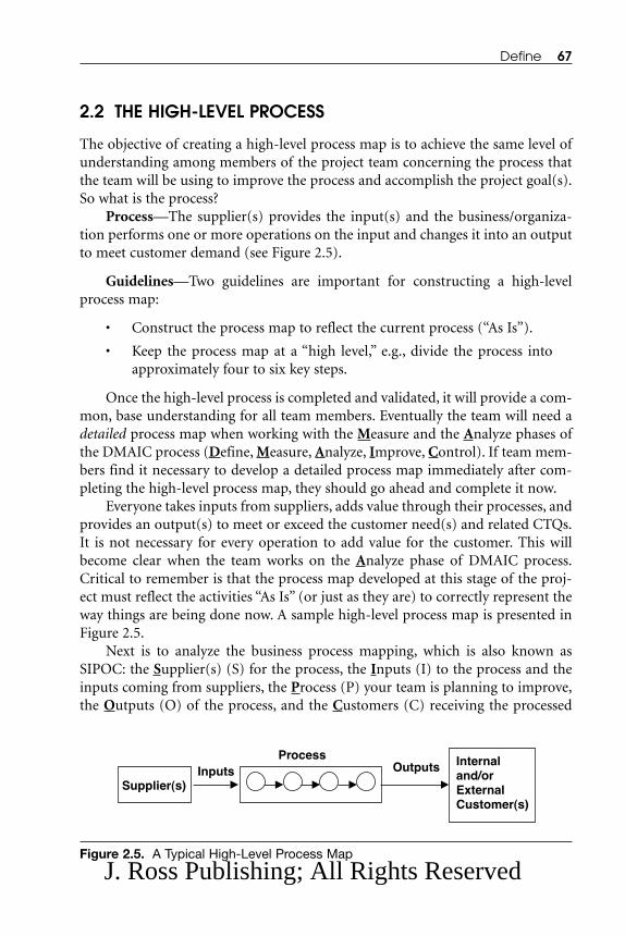
2.2 THE HIGH-LEVEL PROCESS
The objective of creating a high-level process map is to achieve the same level ofunderstanding among members of the project team concerning the process thatthe team will be using to improve the process and accomplish the project goal(s).So what is the process?
Process—The supplier(s) provides the input(s) and the business/organiza-tion performs one or more operations on the input and changes it into an outputto meet customer demand (see Figure 2.5).
Guidelines—Two guidelines are important for constructing a high-levelprocess map:
• Construct the process map to reflect the current process (“As Is”).
• Keep the process map at a “high level,” e.g., divide the process intoapproximately four to six key steps.
Once the high-level process is completed and validated, it will provide a com-mon, base understanding for all team members. Eventually the team will need adetailed process map when working with the Measure and the Analyze phases ofthe DMAIC process (Define, Measure, Analyze, Improve, Control). If team mem-bers find it necessary to develop a detailed process map immediately after com-pleting the high-level process map, they should go ahead and complete it now.
Everyone takes inputs from suppliers, adds value through their processes, andprovides an output(s) to meet or exceed the customer need(s) and related CTQs.It is not necessary for every operation to add value for the customer. This willbecome clear when the team works on the Analyze phase of DMAIC process.Critical to remember is that the process map developed at this stage of the proj-ect must reflect the activities “As Is” (or just as they are) to correctly represent theway things are being done now. A sample high-level process map is presented inFigure 2.5.
Next is to analyze the business process mapping, which is also known asSIPOC: the Supplier(s) (S) for the process, the Inputs (I) to the process and theinputs coming from suppliers, the Process (P) your team is planning to improve,the Outputs (O) of the process, and the Customers (C) receiving the processed
Define 67
Supplier(s)Inputs
ProcessOutputs Internal
and/orExternalCustomer(s)
Figure 2.5. A Typical High-Level Process Map
J. Ross Publishing; All Rights Reserved

outputs. A SIPOC diagram is presented in Figure 2.6. The terms in SIPOC can bedefined as:
• Supplier—A source or a group of sources that provides the inputs toprocess
• Input—Resources (e.g., equipment, facility, material, people, technol-ogy, and utilities) and information (i.e., data) required to execute theprocess/operation(s).
• Process—A collection (series) of operations (activities) that is per-formed over one or more inputs that produces the output to meetcustomer demand (Note: The limits of a particular process or theProcess Boundary are usually identified by the inputs and the outputsas outside the process boundary.)
• Output—The tangible product or service that results from the processto meet customer demand
• Customer (internal and/or external)—An individual and/or organi-zation receiving the processed output (Remember: CTQs are the per-formance standards of critical measurable characteristics of a processor product that must be met to satisfy the customer.)
The SIPOC tool is especially useful when certain information is unclear:
• Who supplies inputs to the process?
• What specifications (CTQs) are placed on the inputs?
• Who are the true owners of the process?
• Who are the true customers of the outputs?
• What are the requirements (CTQs) of the customers?
Following these steps allows completion of the SIPOC diagram:
1. Begin with the process and map it in four to five high-level activities.
2. Identify the outputs of this process.
3. Identify the customers who will receive the outputs of this process.
68 Six Sigma Best Practices
Supplier
Internalor
External
CTQs CTQs Internalor
External
Input Process Output Customer
Figure 2.6. SIPOC Chart
J. Ross Publishing; All Rights Reserved

4. Identify the inputs required for the process to function properly.
5. Identify the suppliers of the inputs.
6. Discuss with project sponsor, champion, and other involved stake-holders for verification.
Not required, but useful, is identifying the preliminary requirements (CTQs)of the customers. This will be verified during the Measure phase of the DMAICprocess.
As an example, consider Tractor Dealer XYZ, in which manufacturers supplythe product (tractors and accessories) and other suppliers provide the elementsrequired to operate the dealership and support customers (e.g., diesel fuel, repairtools, cleaning supplies, etc.). Farmers purchase tractors and support productsfrom the tractor dealership. The dealer makes financial arrangements for farmers(buyers) with financial institutions (banks). Farmers define tractor specificationsto meet their needs. There is one exception: farmers have no color option for trac-tors. Each tractor manufacturer has its own defined color; all tractors from a spe-cific manufacturer are painted the same color. The SIPOC diagram for TractorDealer XYZ is presented in Figure 2.7.
2.3 DETAILED PROCESS MAPPING
The process mapping concept is applicable to both product and service organiza-tions. Advantages of process mapping include:
• Easy visualization of the total process
• Easy analysis of the total process
• Easy identification of non-value added and waste activities
• Easy communication of the impact of process improvement
• Easy identification of the process cycle time for each operation andfor the total process
Next is developing the business process map. The concept is similar to thehigh-level process map, but each process section is mapped in more detail. Keysteps in mapping and analyzing the business process flow chart include:
1. Define and name the process to be mapped. Establishing the startand stop points of a process is a critical first step in process mapping.Typically, the start point of a process is the first step that receivesinputs from suppliers and the end point is delivery of the product orservice to the customer.
Define 69
J. Ross Publishing; All Rights Reserved

2. Familiarize the team (participants) with the flow chart symbols.
3. Identify customer needs (CTQs) and outputs. Survey and convertcustomer needs into customer CTQs. Output must satisfy thoseCTQs on demand (on time).
4. Identify the process steps. Identify the sequence of process activities.Draw the process and diagram the flow consistently from top to bot-tom or from left to right.
5. Identify a decision point or branch point. Choose one branch andcontinue flow diagramming.
6. Identify the process that is unclear or unfamiliar to team members.Make a note and continue flow diagramming.
70 Six Sigma Best Practices
Suppliers
CTQs
Inputs Processes Outputs Customers
• ABC Mfg. Co. • Diesel Fuel
Supplier• Other
Suppliers• Tractor Wash
Facility
• Tractors• Option
Packages• Diesel for
Tractors• Tractor
Wash• Tractor Work
Sheet
See Below • New Farmer Account
• Paperwork to State
• Paperwork to Manufacturer
• Paperwork to Dealer
• Payment• Service
Contract• Service
Notification
• Tractor Buyer (Farmer)
• Dealership Owner
• State Tax Department
• Service Department
Step 1:Meet with new client (farmer)
Step 2:Understand farmer’s needs in new tractor
Step 3:Present options to farmer and negotiate price
Step 4:Agree on options, price, and delivery date
Step 5:Sign paperwork, payment arrangement, and hand over keys and title
• Tractor Meets Specifications
• Options Package• Special Tool Box
CTQs
• Build to Order • Loan Approval • Bank Check
Figure 2.7. SIPOC Diagram for Tractor Dealer XYZ
J. Ross Publishing; All Rights Reserved

7. Brainstorm the major steps (tasks) in the work process. Do not beconcerned about the sequence at this point. Ask questions such as“What really happens next in the process?” and “Does a decisionneed to be made before the next step?” and “What approvals arerequired before moving on to the next task?”
8. Repeat Steps 4 through 7 until the team reaches the last (or first) stepin the process.
9. Go back and flow diagram the other branches.
10. Put the steps in the proper sequence. As this is done, the team maybegin to add minor points as necessary. At this point, all the stepshave been identified and sequenced. Now assign the appropriatesymbols to each step (see the discussion in the Flow Charting sectionof Chapter 3) and connect the steps with arrows to show the flow ofthe process.
11. Identify critical inputs. Some inputs may be required at the begin-ning of the process, while others may be required during the process.
12. Identify each supplier from which the process owner receives eachinput.
13. Validate process map. To validate the map, make sure that theprocess is represented “As Is.” Now work on process validation withkey stakeholders and/or with functions that perform the processsteps. A process has three possible versions:
• What you think it is—One that is based on the individuals whotouch the process.
• What it really is—One that is based on reconciling what theprocess map really is. The consolidation of the first two versionsof the process map constitutes what is referred to as the “As Is”process map. The effectiveness of the next two phases, Measureand Analyze, will depend on the accuracy and detail of theprocess map.
• What it should be—As the team moves forward and conductsprocess analysis and problem solving, the third version of theprocess map—the “should be” map—is developed. Critical atthis point is to check if the output from this process is meetingor exceeding the customer needs/requirements or if it is not.
As the team analyzes the process activities, the team should also try to deter-mine answers for the following:
• Each decision point:
– Is this a checking activity?
– Is this a redundant check?
Define 71
J. Ross Publishing; All Rights Reserved
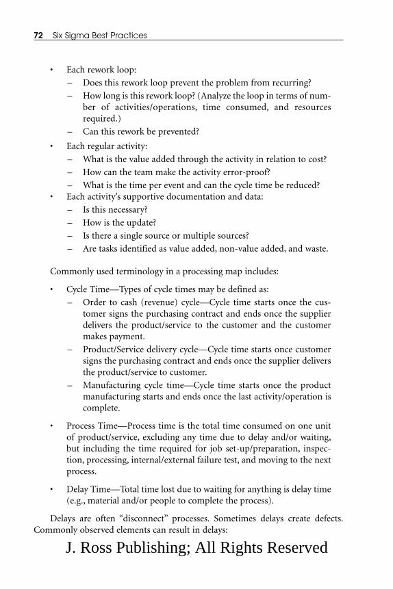
• Each rework loop:
– Does this rework loop prevent the problem from recurring?
– How long is this rework loop? (Analyze the loop in terms of num-ber of activities/operations, time consumed, and resourcesrequired.)
– Can this rework be prevented?
• Each regular activity:
– What is the value added through the activity in relation to cost?
– How can the team make the activity error-proof?
– What is the time per event and can the cycle time be reduced?• Each activity’s supportive documentation and data:
– Is this necessary?
– How is the update?
– Is there a single source or multiple sources?
– Are tasks identified as value added, non-value added, and waste.
Commonly used terminology in a processing map includes:
• Cycle Time—Types of cycle times may be defined as:
– Order to cash (revenue) cycle—Cycle time starts once the cus-tomer signs the purchasing contract and ends once the supplierdelivers the product/service to the customer and the customermakes payment.
– Product/Service delivery cycle—Cycle time starts once customersigns the purchasing contract and ends once the supplier deliversthe product/service to customer.
– Manufacturing cycle time—Cycle time starts once the productmanufacturing starts and ends once the last activity/operation iscomplete.
• Process Time—Process time is the total time consumed on one unitof product/service, excluding any time due to delay and/or waiting,but including the time required for job set-up/preparation, inspec-tion, processing, internal/external failure test, and moving to the nextprocess.
• Delay Time—Total time lost due to waiting for anything is delay time(e.g., material and/or people to complete the process).
Delays are often “disconnect” processes. Sometimes delays create defects.Commonly observed elements can result in delays:
72 Six Sigma Best Practices
J. Ross Publishing; All Rights Reserved

• Bottlenecks—Any location where assigned load is equal to or greaterthan available capacity.
• Conflicting objectives—The goals of one group can create problemsor errors for another group, e.g., when one group is focusing onprocess speed while another group is concentrating on error reduc-tion. One result may be that neither group accomplishes its objectives.
As the team continues to analyze the process map, other issues the team mayencounter include:
• Common Problem Areas—This situation can occur when opera-tions/activities are repeated at several locations in a process, e.g., arotational part for a jet engine may go through two to four turningmachines as part of the rough turning operation before it moves onto the finishing operation. These locations can provide insight intopotential solutions. The team should encode these “disconnects” andhighlight them directly on the process map.
• Gaps—The process seems to go off track or the defined process for agiven activity is unclear or wrongly interpreted.
• Redundancies—If more than one group is responsible for the process,redundancies can occur when different groups take action, but areunaware that actions are being taken elsewhere in the process byanother group.
Process mapping is a special situation of flow charting. The flow-chartingconcept will be discussed further in the Measuring Tools section of Chapter 3(Measure). If the team leader was not in a position to develop the project charterat the end of Chapter 1, he/she must be in a position to develop one now.
Before moving on, consider Exercise 2.2.
Exercise 2.2: Develop a High-Level Process Map
As a class project, develop a high-level process map that includes:
• What is the name of the process?
• What are the outputs?
• Who are the customer(s) of those outputs?
• What are the inputs and their suppliers?
• Process:
– Start point
– End (completion) point
Define 73
J. Ross Publishing; All Rights Reserved
– First operation (activity)
– Last operation (activity)
2.4 SUMMARY
This chapter has been a continuation of the discussion of the Define phase of theDMAIC process. Key topics discussed in this chapter include:
• Customer definition—internal, external, and stakeholders
• Critical to quality characteristics (CTQ)
• Research customer
• Customer research methods
• Customer feedback
• Key steps of a total process from supplier through customer (SIPOC)
• Key definitions of the total process elements
• Process mapping
The project team must check customers and CTQs and business process map-ping before proceeding to Chapter 3:
Customers and CTQs:
• Has the customer(s) been identified?
• Has the improvement team collected the “voice of the customer”(obtained feedback qualitatively and quantitatively)?
• What customer feedback methods were used to solicit customerinput?
• Have the customer needs and requirements been translated into spe-cific, measurable requirements?
Business Process Mapping:
• Have high-level and “As Is” process maps been completed, verified,and validated?
• Has a SIPOC diagram been developed describing the suppliers,inputs, process, outputs, and customers?
• Is the project team aware of the different versions of process maps,e.g., what the team thinks the process is vs. what the process actuallyis?
74 Six Sigma Best Practices
J. Ross Publishing; All Rights Reserved

• Is the current “As Is” process being followed? If not, what are the dis-crepancies?
• What procedure was used to develop, review, verify, and validate the“As Is” process map?
• What tools and methodology did the team use to get through theDefine phase?
REFERENCES
1. Juran, J.M. 2002. Juran Institute’s Transactional BreakthroughStrategy. Southbury, CT: Juran Institute. Chapters 1 and 2 fromnotes given to students in a Black Belt certification training class.
ADDITIONAL READING
Juran, J.M. and A.B. Godfrey. 1999. Juran’s Quality Handbook, FifthEdition New York: McGraw-Hill.
The Juran Institute. 2002. The Six Sigma Basic Training Kit. New York:McGraw-Hill.
Define 75
This book has free material available for download from theWeb Added Value™ resource center at www.jrosspub.com
J. Ross Publishing; All Rights Reserved

J. Ross Publishing; All Rights Reserved

3
MEASURE
Process definition and data collection plans build validity and consistency intodata. Data reflect process performance and provide insight and knowledge abouta process. If a team wants to evaluate variation in a process, it will need to collectdata. A data collection system is a type of measurement system.
Any business or organization must know “where it stands” currently if it isattempting to achieve a defined goal(s). Six Sigma uses a measurement system toestablish a baseline, which will identify where a product/service is in relationshipto defined goals. To establish a baseline, current measurements are needed. Oncea business knows where it is and where it wants to go, existing gaps can be deter-mined and the business can also assess the efforts and resources needed to reducethe gap(s) in product/service quality and thereby achieve the goal(s).
77
Define
Measure
Analyze
Improve
Control
J. Ross Publishing; All Rights Reserved
Think about the SIPOC process (Supplier-Input-Process-Output-Customer), in which measurement occurs at three different stages of theprocess—inputs, process, and outputs.
Input measures represent measures of the key CTQs (critical to quality char-acteristics) placed on suppliers. Input measures indicate supplier performanceand also correlate to output measures. Input measures are defined as independentvariables and are represented by the letter X. Process measures are internal to theprocess and include key control elements for improving the output measures.Output measures are defined as dependent variables and are represented by theletter Y. Meaningful process measures will correlate with output measures. Theletter Y also represents process measures.
Output measures are used to determine how well customers’ CTQs are beingsatisfied. Independent variables are represented by Xs; dependent variables arerepresented by Ys. When appropriate independent variables are measured andtracked, they can be used to predict the dependent (Y) variable. The relationshipis presented as:
Y = f (X1, X2, X3, …, Xn)
where one dependent variable (Y) is a function of (dependent on) n independentvariables (X1, X2, X3, …, Xn). Once the project has a clear definition with a clearmeasurable Y, the process is studied to determine the key process steps and the keyinputs for each process. The team will analyze the potential impact of each inputwith respect to the variation of the project Y. Inputs are then prioritized to estab-lish a short list to study in more detail how these inputs can “go wrong.” Once thecause for input failure is determined, a preventive action plan can be put intoplace. Discussion in this chapter will be limited to current data collection, datacollecting tools, how to present data, some basic probabilistic distributions repre-senting the data and their application, and a discussion of process capability.
Chapter topics include:3.1 The Foundation of Measure
3.1.1 Definition of Measure3.1.2 Types of Data3.1.3 Data Dimension and Qualification3.1.4 Closed-Loop Data Measurement System
3.2 Measuring Tools3.2.1 Flow Charting3.2.2 Business Metrics3.2.3 Cause-and-Effect Diagram3.2.4 Failure Mode and Effects Analysis (FMEA) and Failure Mode,
Effects, and Criticality Analysis (FMECA) 3.2.4.1 FMECA
78 Six Sigma Best Practices
J. Ross Publishing; All Rights Reserved

3.2.4.2 Criticality Assessment3.2.4.3 FMEA3.2.4.4 Modified FMEA
3.3 Data Collection Plan3.4 Data Presentation Plan
3.4.1 Tables, Histograms, and Box Plots3.4.2 Bar Graphs and Stacked Bar Graphs3.4.3 Pie Charts3.4.4 Line Graphs (Charts), Control Charts, and Run Charts3.4.5 Mean, Median, and Mode3.4.6 Range, Variance, and Standard Deviation
3.5 Introduction to MINITAB®3.6 Determining Sample Size3.7 Probabilistic Data Distribution
3.7.1 Normal Distribution3.7.2 Poisson Distribution3.7.3 Exponential Distribution3.7.4 Binomial Distribution3.7.5 Gamma Distribution3.7.6 Weibull Distribution
3.8 Calculating Sigma3.9 Process Capability (Cp, Cpk) and Process Performance (Pp, Ppk)
Indices3.10 SummaryReferences
3.1 THE FOUNDATION OF MEASURE
Every product/service goes through three stages of the SIPOC process—input,process, and output—as presented in Figure 3.1. These three stages are also criti-cal stages for measurement. As identified earlier, output is dependent on inputand process. There may be a variety of inputs that may go through the process toproduce an output to meet customer needs on time. Inputs could be people,material, a machine, a procedure, an environment, etc. An example of inputs, inprocess, and outputs is presented in Example 3.1.
Example 3.1: Stages of an Architect’s House Design Services
Identify stages for an architect’s house design services and classify the variablesinto independent and dependent categories.
The architect’s services can be divided into three stages—input, in process,and output. Variables for each stage are classified as:
Measure 79
J. Ross Publishing; All Rights Reserved

• Input—Customer needs and wants are independent variables:
– X1—Master bedroom
– X2—Daughter’s bedroom
– X3—Son’s bedroom
– X4—Guest bedroom
– X5—Master bedroom bathroom
– X6—Main bathroom
– X7—Guest bedroom bathroom
– X8—Living room space
– X9—Kitchen and dining space
– X10—Extra storage space in kitchen
– X11—Sunlight windows in the ceiling
• In Process—Output is dependent on input and in process variables:
– X20—Total bedroom space
– X21—Total bathroom space
– X22—Total hallway space
– X23—House entrance space
– X24—Utilities space
80 Six Sigma Best Practices
CTQs CTQs Internalor
External
Internalor
External
Measures Measures
Measure In Process Flow
CustomerOutputProcessInputSupplier
Figure 3.1. Measures in SIPOC Chart
J. Ross Publishing; All Rights Reserved

• Output—The architect’s service output must meet the customer’sCTQs:
– Y1—House layout
– Y2—House material requirements
– Y3—House construction cost
All outputs may not be the same, i.e., there may be some variation in outputs.The next step is to investigate the sources of variation. There are two sources ofvariation—common cause and special cause.
Common cause is due to inherent interaction among input resources.Common cause is predictable, random, and normal. Analyze the key possiblevariations and improve solutions based on these variations. Key to minimizingcommon cause is focusing on fundamental process change.
Special cause is due to especially large influence by one of the input resources.Special cause is generally unpredictable and abnormal. Investigate specific meas-urements (data points) related to the special cause. Develop solution(s) for thespecial cause, implement the most appropriate solution, and measure again. Keyto minimizing special cause is focusing on investigating special causes.
To develop a sound strategy for process control and improvement, and cus-tomer satisfaction, it is important to understand the sources of variation.Appropriately responding to the source of variation in a process provides the cor-rect economic balance, as opposed to overreacting or underreacting to variationfrom a process.
If the process shows common cause variation, investigate all the data points.It is difficult to relate common cause variation to a few causal input factors (Xs).If there is a common cause variation, then focus on fundamental process change.(A detailed analysis will be presented in the Analyze phase of the DMAIC processin Chapter 4, Analyze.)
If the process shows special cause variation, the appropriate action is to inves-tigate those specific data points related to the special cause signals. In most cases,the analysis will show the relationship. The results should be integrated into anaction plan as quickly as possible to address the special cause.
To build a strong foundation for measure, understanding Sections 3.1.1,3.1.2, 3.1.3, and 3.1.4 is important.
3.1.1 Definition of MeasureMeasurement is a procedure that provides the most general approach to any phys-ical problem. Measure is a reference standard used for the quantitative comparisonof properties. For a process or population of a product/service, measure describes:
• Dimension
Measure 81
J. Ross Publishing; All Rights Reserved

• Surface
• Capacity
• Performance
• Quality
• Characteristics
Sample units of measure include:
• Product dimension—Inches, feet, and centimeters
• Product manufacturing cycle time—Hours, days, and weeks
• Product heat-treating surface—Square inches
• Product holding capacity—Gallons
• Product characteristics—Tight tolerances, surface hardness
• Product performance—Miles per gallon
Effectiveness and efficiency are two types of measures:
• Effectiveness of measures—Any process/system is meeting andexceeding the customer needs and requirements, e.g., service responsetime, percent product defective, and product functionality.
• Efficiency of measures—Any process/system is meeting and exceedingthe customer requirements based on the amount of the resources allo-cated, e.g., product rework time, product cost, and activity time.
Measure can be qualitative or quantitative:
• Qualitative measure—A variable that normally is not expressednumerically is measured qualitatively. These variables differ in type,e.g., qualitative variables are sex, race, job title, etc. Qualitative vari-ables can be subdivided into two categories—dichotomous qualitativevariables and multiqualitative variables.
– Dichotomous qualitative variables—These variables can be inonly two categories, e.g., male or female, employed or unem-ployed, correct or incorrect, defective or satisfactory, elected ordefeated, absent or present, etc.
– Multiqualitative variables—These variables can be in more thantwo categories, e.g., job titles, colors, languages, religions, type ofbusinesses, etc.
• Quantitative measure—A variable that is normally expressed numer-ically is measured quantitatively. These variables differ in degree, e.g.,
82 Six Sigma Best Practices
J. Ross Publishing; All Rights Reserved

years of service, annual salary, etc. (Most of the discussion in thisbook will be related to quantitative measure.) Quantitative variablescan be subdivided into two categories—discrete variables and contin-uous variables:
– Discrete variables—A discrete variable is based on counts. Someof the measurement observations fall in this category with a finitenumber of possible values, but the values cannot be subdividedmeaningfully, e.g., the number of unacceptable parts in thereceived shipment.
– Continuous variables—A continuous variable has a large numberof values with no special category label attached to any particulardata value. Data can conceptually take on any value inside someinterval. Continuous data are the actual measurement values, e.g.,the amount of time to complete a task, the distance between twopoints, etc.
3.1.2 Types of Data The assignment of numbers to characteristics that are being observed (i.e., col-lected), which is also a measurement, can yield four types of data of increasingcomplexity:
• Nominal data
• Ordinal data
• Interval data
• Ratio data
Nominal DataThe weakest level of measurement produces nominal data. These numbers aremerely names or labels for different things and thus can serve the purpose of clas-sifying observations about qualitative variables into mutually exclusive groups,e.g., “night” might be numbered as 0 and “day” as 1, but alternative labels of“night” = 10 and “day” = 3 would serve as well. Other examples of creating nom-inal data would be classifying defective units of a product as “0,” good (nondefec-tive) units as “1,” or labeling houses on a street with 10, 21, 30, 41, etc. Theseexamples confirm that it never makes sense to add, subtract, multiply, or dividenominal data, but these numbers can be counted. If there are five 0s based on theabove-defined defective code, then there are five defective units.
Measure 83
J. Ross Publishing; All Rights Reserved
Ordinal DataThese numbers are by their size order or they rank observations on the basis ofimportance, while intervals between the numbers or the ratio of such numbers aremeaningless, e.g., assessments of a product as great, good, average, and poor mightbe recorded as 4, 3, 2, 1 or 10, 8, 6, 5. The important point is that larger numbersdenote a more favorable assessment or a higher ranking, while smaller onesdenote the opposite. Ordinal data make no statement about how much more orless favorable one assessment is compared to another. A 4 is deemed better than a1, but not necessarily 4 times as good; a 100 is deemed better than a 10, but notnecessarily 10 times as good; a 3 is deemed worse than 9, but not necessarily athird as good. Teaching staff titles at any university of professor, associate profes-sor, and assistant professor, with an ordinal coding as 3, 2, and 1, is simply a cod-ing and does not imply that, in some sense, professors are viewed as moreimportant than assistant professors. Similarly, a nominal coding of male = 10,female = 3 does not imply the superiority of males over females any more than acoding of male = 1, female = 4 denotes the opposite. There are no arithmeticoperations with the data.
Interval DataInterval data are somewhat more sophisticated. These data allow at least additionand subtraction. Interval data are numbers that by their size rank observations inorder of importance and the distance or interval between the points is compara-ble, but their ratios are meaningless. Because these data do not possess an intrin-sically meaningful origin, their measurement starts from an arbitrarily locatedzero point and utilizes an equally arbitrary unit distance for expressing intervalsbetween numbers. Commonly used examples of interval data are temperaturescales. The Celsius scale places 0 at the water-freezing point and places 100 at thewater-boiling point. The Fahrenheit scale places 0 far below the water-freezingpoint in Celsius and the water-boiling point is far above the Celsius water-boilingpoint. Within the context of either scale, the unit distance (degree of temperature)has a consistent meaning. Each degree Celsius equals 1/100 of the distancebetween water’s freezing and boiling points; similarly, each degree Fahrenheitequals 1/180 of that distance. An interesting point is that zero, being arbitrarilylocated, does not denote the absence of the characteristic being measured. Alsonote that any ratio of the corresponding Celsius figures (for 45°F and 10°F) doesnot equal to 3:1, but for Fahrenheit, the ratio is well over 4:1.
Ratio DataRatio data (numbers) are the most sophisticated data. Ratio data are the most use-ful type of data and can be ranked by:
84 Six Sigma Best Practices
J. Ross Publishing; All Rights Reserved

• Size—Size ranks data observations in order of importance andbetween which intervals. All types of arithmetic operations can beperformed with each datum because these numbers have a natural ortrue zero point that denotes the complete absence of the characteris-tic they measure and makes the ratio of any two such numbers inde-pendent of the unit of measurement.
• Importance—Ratio data are meaningful data, e.g., the measurementof distance, height, area, volume, or weight produces ratio data. As anexample, it is meaningful to rank height data and to say that a 20-footpole is taller than one of 10 feet, which is taller than one of 5 feet. Poledata give the kind of ordinal data information. It is also meaningful tocompare intervals between pole height data: it is easy to say that thedistance between 20-foot and 10-foot poles is two times the distancebetween 10-foot and 5-foot poles. Furthermore, these data are ratiodata because it can safely be stated that a 15-foot pole is three timestaller than a 5-foot pole. Even if the unit of measurement is changed,e.g., from feet to inches or from feet to yards, this conclusion does notchange.
3.1.3 Data Dimension and QualificationNext in data measurement is identifying data dimension and qualification.Identifying data dimensions (or units) is important. Data dimensions supportactivities such as data collection and analysis, process validation, quality improve-ments, etc. Remember from Section 3.1.1 that the qualitatively measured variablesdiffer in type, e.g., sex, race, job title, etc. and that there are no established units ofmeasurement (a unit). The quantitatively measured variables involve both a num-ber and a standard of comparison, e.g., 3 feet, 5 pounds, and 25 minutes are thenumbers and the standard of comparison (i.e., feet, pound, or minute) is arbitrar-ily established and is called a unit.
Abstract data must be broken down into identifiable and measurable data.For example, appearance of the entrance lobby of an office building is certainly aquality feature, but it also looks like an abstraction. The features need to bedivided into observable parts and identified into those specifics that collectivelyconstitute appearance, e.g., the quality and condition of the carpet, the qualityand style of furniture, the size of windows, etc. Once data dimensions have beenestablished for each piece or item, the team should summarize the data into anindex, e.g., number of damaged or soiled carpets to total number of office rooms,number of rooms with old and damaged furniture, etc.
Data are also qualified/classified based on local environment, applications,and decision-making. Classifications include:
Measure 85
J. Ross Publishing; All Rights Reserved
• Broadly applicable—Some data dimensions that are broadly applica-ble can help to answer such questions as:
– Is the product/service quality getting better or worse?
– Which one of the products/services provides the best quality?
– How can all of the business operations be brought up to the bestlevel?
• Common basis of decision making—Measurement units should besuch that the data will provide assistance for a decision-making groupmade up of diverse people.
• Compatibility—Sometimes data are measured in simple units toapply to a wide variety of situations.
• Economical to apply—There must be balance between the cost of col-lecting data and the benefits of having the data. Sometimes data pre-cision also relates to marginal benefits.
• Measurable in abstraction—Some quality features stand apart fromphysical things (are subjective), e.g., taste, feel, sound, aroma, andbeauty.
• Understandable—Technological data generally have highly standard-ized dimensions. However, the dimensions of managerial level dataare not standardized. Local dialects may be understood by local busi-ness people, but not by outsiders, e.g., world-class quality, on-timearrival, etc. These types of measurement qualifications are vagueand/or create confusion that can divide the team.
3.1.4 Closed-Loop Data Measurement SystemMany measurement systems follow the closed-loop system concept due to lowercomputing costs and great technological growth. As an example, consider thethermostat control in a heating and/or cooling system. The quality of this deviceneeds to be evaluated. One of the key elements in making the evaluation is thesensor. A sensor is a specialized detecting device or measurement tool. It isdesigned to recognize the presence and intensity of certain phenomena and toconvert this sensed knowledge into information. In turn, the resulting informa-tion becomes an input to decision-making, enabling the team to evaluate theactual performance. (Similarly to technological instruments, which obviouslyhave sensors, humans and animals use their senses the same way.) A closed-loopsystem generally follows four key steps:
• Data recording—As a system is functioning, defined data are measured.
• Data processing—Measured data are processed. This processing mayhappen within same system or outside the measuring system.
86 Six Sigma Best Practices
J. Ross Publishing; All Rights Reserved

• Comparing data—The processed performance data are comparedwith goals and standards.
• Actuating—The control system adjusts the processes to bring per-formance into conformance with standards.
The project team will handle two types of data to measure and appreciate thesize of performance problem(s) (as defined in Section 1.10, Project Charter, inChapter 1):
• Dependent data—Also known as “Ys”
• Independent data—Also known as “Xs”
Several techniques are available to identify the Ys data—brainstorming, busi-ness metrics, a data selection matrix, and a performance measure matrix. Theselected Ys data must satisfy certain requirements. They must be:
• Consistent with project charter
• Consistent with customer expectations
• Supportive of business strategy, i.e., business goals, competitors,benchmarking, existing specifications, and regulations (national/international)
Once the selected list is developed, apply the following criteria to select thehighest-ranking Ys:
• Y is measurable.
• Y must be linked to customer CTQs.
• Y is a direct measure of the process.
• Y addresses the process defect problem.
• Volume of the product or process is large enough to support theimprovement project.
• Data on Y are easy to collect.
• Cost of product failure is high.
• Continuous data (generally) are preferable over discrete data.
A ranking matrix can be developed utilizing the concept of assigned numbersthat can range from 1 through 10, with 10 meeting the criteria perfectly and 1 notmeeting the criteria at all.
Similarly, there are several techniques available to identify the Xs data, e.g.,brainstorming, process mapping, and cause-and-effect diagrams. Key considera-tions in selecting Xs are the elimination/minimization of variation and that theselected Xs must be measurable. Measurement occurs at three stages of the SIPOC
Measure 87
J. Ross Publishing; All Rights Reserved
process—inputs, process, and outputs—therefore, identify potential project Xsthat will be measured in the data collection plan. The selected Xs should be pri-oritized utilizing commonly available tools such as:
• Prioritization matrix
• Failure mode effect analysis (FMEA)
Next is creating a matrix relating the Xs and the Ys variables:
• List the selected project Ys along the top section of the matrix.
• Assign weight to each project Y (generally using 0 through 5), with themost important output receiving the highest number.
• List all potential causes (inputs) from this process and cause-and-effect analysis that can impact the various project Ys along the left-hand side of the matrix.
• Quantify the effect of each input on each project Y in the body of thematrix.
• Use the results to analyze and prioritize the team’s focus and data col-lection.
Numerous tools are available to measure data, but only a few will be discussedin Section 3.2, Measuring Tools. Before moving on, consider Exercise 3.1.
Exercise 3.1: A Class Project
What is the registration process for entering freshmen students at the Universityof New Haven (or any selected university)?
• Develop a process flow chart.
• Brainstorm opportunities.
• Review CTQs for the project.
• Develop project information based on applicable elements:
– Possible process activities
– Measurable?
• Unit of measure
• Frequency of measurement
– Opportunity defined?
– Linked to CTQs?
– High-priority issue?
– Cost of failure?
– Easy to collect data?
– Data type?
• Appoint a spokesperson to report to class.
88 Six Sigma Best Practices
J. Ross Publishing; All Rights Reserved

3.2 MEASURING TOOLS
Several applicable tools are available in the literature to eliminate obvious causesof variation in the performance of the selected project, therefore only flow chart-ing, business metrics, the cause-and-effect diagram, and FMEA and FMECA (fail-ure mode, effects, and criticality analysis) will be discussed in this section.
3.2.1 Flow ChartingFlow charting is a quality improvement tool specifically used for process analysis,understanding, presentation, and improvement. Flow charts tend to provide userswith a common language or reference point for a project or process. A flow charthas several definitions:
• A flow chart is a pictorial representation of a process in which all thesteps of the process are presented.
• A flow chart is a planning and analysis tool. It is a graphic of the stepsin a work process.
• A flow chart is a formalized graphic representation of a work orprocess, programming logic sequence, or similar formalized proce-dure.
Uses of process mapping (a special-case flow chart described in Chapter 2,Define) may be summarized. Uses include:
• To visualize how an entire process works
• To define and analyze processes, e.g., “What is the registration processfor entering freshmen students at the University of New Haven?” or“How can an invoice be created?”
• To build a step-by-step picture of the process for analysis, to identifythe critical points, bottlenecks, and problem areas in a process or forcommunication purposes, e.g., “Is it possible to shorten the length oftime it takes for a student to complete the program?”
• To see how the different steps in the process are related and then todefine, standardize, or find areas for improvement in the process
• To identify the “ideal” flow of a process from start to finish
• To design a new work process
Although there are various types of flow charts, three types are commonlyused in process analysis:
Measure 89
J. Ross Publishing; All Rights Reserved

• Top-down flow chart—This chart starts with the major steps drawnhorizontally. The detail is provided in numbered subtasks under eachmajor task. The top-down flow chart does not show decision pointsand reworks. Therefore, it is not as detailed as a process or deploy-ment flow chart.
• Detailed process flow chart—This chart is also known as processmapping. It has been discussed previously (see Chapter 2) and it ismost useful when analyzing a specific function, activity, or process.
• Deployment flow chart—This chart is useful when analyzing aprocess that involves more than one group or several individuals.When a process calls for a deployment flow chart, it may first be help-ful to construct a process flow chart with only the major steps andthen modify it by assigning the appropriate groups or individuals toeach step.
Process flow charts should divide the process into two stages:
• The product’s manufacturing process—Typically incorporates alltypes of manufacturing, assembly, and test operations
• The finished product process—Incorporates other activities associ-ated with the product, e.g., transporting the product
These two stages of the process should be considered using separate flow charts.
The Manufacturing Process Flow ChartGenerally ANSI (the American National Standards Institute) standard symbolsare used. The most commonly used symbols are presented in Figure 3.2A.Examples of terms within the symbols include:
• Operation—Material turning, grinding, pouring cement, buildinghouse structure, and typing e-mail
• Transportation—Moving material using a transport vehicle (truck,fork truck, etc.), conveyor belt, and manually
• Storage—Storing material (raw, work-in-process, and finished) incontainers, pallets, etc. or storing filed documents
• Delay—Material is waiting at the processing machine (turning, grind-ing) for documentation, inspection, etc. or material is waiting to usean elevator
• Inspection/Measurement—First-piece checking on a manufacturingmachine to meet specifications and product quality, reading docu-ments for the accuracy of stored information, and reading gauges
• Combined Activities—Two combined activities such as the jointprocess of operation and inspection
90 Six Sigma Best Practices
J. Ross Publishing; All Rights Reserved

Measure 91
Operation
Transportation
Storage
Delay Inspection/Measurement
Operation/Inspection
Connector Flow Lines
RazorBlade
RazorBladeHolder
PinRazorHandle
Assemble
AssembleHold RazorBlade TopAssembly
FinishedGoods
Figure 3.2A. ANSI Standard Symbols
Figure 3.2B. Razor Blade Assembly Process Flow Chart
J. Ross Publishing; All Rights Reserved
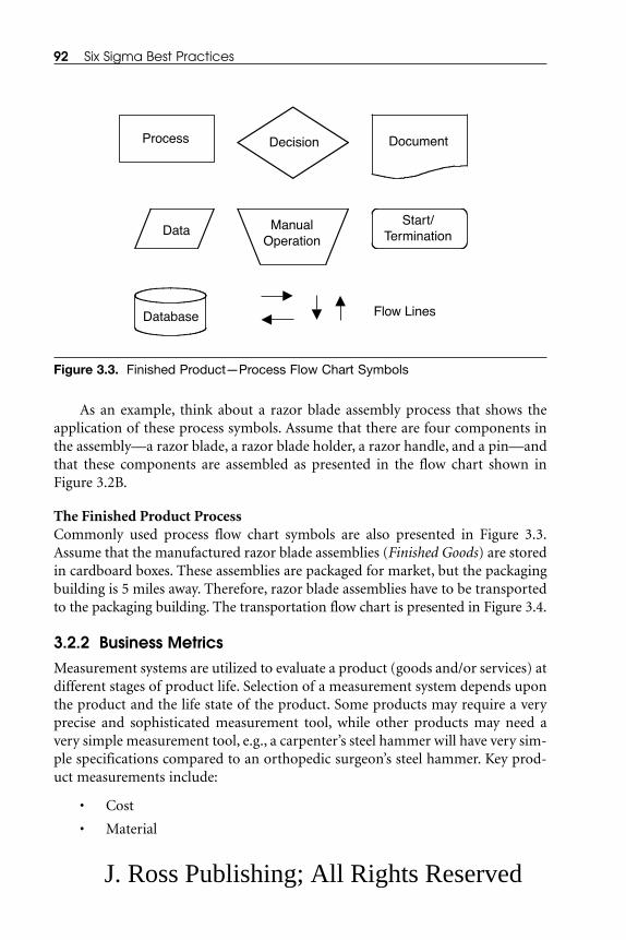
As an example, think about a razor blade assembly process that shows theapplication of these process symbols. Assume that there are four components inthe assembly—a razor blade, a razor blade holder, a razor handle, and a pin—andthat these components are assembled as presented in the flow chart shown inFigure 3.2B.
The Finished Product ProcessCommonly used process flow chart symbols are also presented in Figure 3.3.Assume that the manufactured razor blade assemblies (Finished Goods) are storedin cardboard boxes. These assemblies are packaged for market, but the packagingbuilding is 5 miles away. Therefore, razor blade assemblies have to be transportedto the packaging building. The transportation flow chart is presented in Figure 3.4.
3.2.2 Business MetricsMeasurement systems are utilized to evaluate a product (goods and/or services) atdifferent stages of product life. Selection of a measurement system depends uponthe product and the life state of the product. Some products may require a veryprecise and sophisticated measurement tool, while other products may need avery simple measurement tool, e.g., a carpenter’s steel hammer will have very sim-ple specifications compared to an orthopedic surgeon’s steel hammer. Key prod-uct measurements include:
• Cost
• Material
92 Six Sigma Best Practices
Process Decision Document
Data ManualOperation
Start/Termination
Database Flow Lines
Figure 3.3. Finished Product—Process Flow Chart Symbols
J. Ross Publishing; All Rights Reserved

• Safety and security
• Satisfaction
• Service
• Specifications
• Quantity
• Time
Measure 93
Load AssemblyBoxes in Truck
Check Timeand Weather
Weather Clear?
Before 5:00 PM?
Check for Congestionon Primary Route
Primary RouteCongested?
Use AlternateRoute “B”
Use AlternateRoute “A”
Use PrimaryRoute
Arrive Safely atPackaging Building
Yes
Yes
Yes
No
No
No
Figure 3.4. Transportation Flow Chart—Blade Assemblies
J. Ross Publishing; All Rights Reserved
The effect of operational measures on financial measures (the bottom line) isthe same for all the products. Therefore, the following measurement system analy-sis applies to all products. Three factors account for the power of the operationalmeasures [throughput (T), operating expense (OE), and inventory (I)].1
• First, all three measures are intrinsic to every production process.
• Second, the measures are straightforward, easy to understand, andeasy to apply.
• Third, once the impact of any action on these measures is calculated,the impact on the bottom-line measures can also be determined.
Example 3.2 demonstrates exactly how the operational measures relate to thebottom-line measures of net profit (NP), return on assets (ROA), and cash flow(CF).
Example 3.2: Business Metrics
XYZ is an outsourced messaging center. It packages outgoing messages for cus-tomers. The center has one printer and two inserters. Customer jobs are printedand inserted at the XYZ center. Data for a typical job are as follows:
Average material cost: 8.6 cents per message
Average operating expense: 6.3 cents per message
Average message revenue: 15.8 cents per message
The XYZ messaging center had throughput of 13,900,000 messages last year, withthe following year-end financial status:
Net sales $2,196,200
Cost of messages produced $2,071,100
Total assets (including inventory) $ 925,000
Inventory (book value) $ 53,700
Inventory (material value) $ 40,000
Annual inventory carrying cost 16% per year
Based on this financial status, the following values are known:
Throughput (T) = (Dollars generated through sales) – (Material cost of goods)
= $2,196,200 – $(8.6/100)(13,900,000)
= $2,196,200 – $1,195,400
= $1,000,800Operating expense (OE) = (Total cost of goods) – (Material cost of goods)
= $2,071,100 – $1,195,400
= $875,700
94 Six Sigma Best Practices
J. Ross Publishing; All Rights Reserved

Inventory (I) = Money invested in materials that the business intends to sell= $40,000
Net profit (NP) = Throughput – Operating expense= $1,000,800 – $875,700= $125,100
Return on assets (ROA) = (Net profit)/(Total assets)= ($125,100)/($925,000)= 13.52%
Cash flow (CF) = Available cash= $125,100
Assume that business XYZ is going through some continuous improvementprocesses. These process improvements will impact the operations measures pos-itively. The following analysis will show that their impact on financial measureswill be very significant. The following data are a continuation of the above exam-ple with four process improvement scenarios.
The four process improvement scenarios are:
• Case 1: Assume that throughput increases by 5%, while operatingexpense and inventory remain unchanged.
• Case 2: Assume that operating expense is decreased by 5%, whilethroughput and inventory remain unchanged.
• Case 3: Assume that inventory is decreased by 10%, while throughputand operating expense remain unchanged.
• Case 4: Assume an outstanding continuous improvement process, inwhich throughput is increased by 5%, operating expense is decreasedby 5%, and inventory is decreased by 10%.
Case 1 assumes that throughput increases by 5%, while operating expenseand inventory remain unchanged. Because operating expense is unchanged, boththroughput and net profit increase by 5% of throughput dollars ($1,000,800):
A throughput increase by 5% = $1,000,800 × 5% = $50,040.
New throughput = $1,000,800 + $50,040= $1,050,840
New net profit = $125,100 + $50,040= $175,140
Percent increase in net profit = ($175,140)/($125,100)
= 40% �
Measure 95
J. Ross Publishing; All Rights Reserved

New return on assets = (New net profit)/(Total assets)= ($175,140)/($925,000)= 18.93%
Percent increase in return on assets = (18.93%)/(13.52%)
= 40% �New cash flow = $125,100 + $50,040
= $175,140
Percent increase in cash flow = $175,140/$125,100
= 40% �Case 2 assumes that operating expense is decreased by 5%, while throughput
and inventory remain unchanged.A 5% reduction in operating expense translates to a dollar saving of
5% × $875,700 = $43,785.
New operating expense = $875,700 – $43,785= $831,915.
New net profit = Throughput – New operating expense= $1,000,800 – $831,915= $168,885
Percent increase in net profit = ($168,885)/($125,100)
= 35% �New return on assets = (New net profit)/(Total assets)
= ($168,885)/($925,000)= 18.26%
Percent increase in return on assets = (18.26%)/(13.52%)
= 35% �New cash flow = $125,100 + $43,785
= $168,885
Percent increase in cash flow = 168,885/125,10
= 35% �Case 3 assumes that inventory is decreased by 10%, while throughput and
operating expenses remain unchanged. If inventory is cut by 10%, then the assetbase is reduced by 10% of the inventory book value:
96 Six Sigma Best Practices
J. Ross Publishing; All Rights Reserved

Reduction in inventory book value = 0.10 × $53,700= $5,370
New total asset = $925,000 – $5,370= $919,630
Operating expense will also be reduced because the cost of carrying inventory willbe reduced. Because the inventory carrying cost is 16% per year,
Reduction in operating expense = 0.16 × $5,370= $859
Net profit will increase by the amount of the reduction in operating expense:
New net profit = $125,100 + $859= $125,959
Therefore, there is a one time inventory reduction of $5,370 and an annual oper-ating expense reduction of $859.
New return on assets = (New net profit)/(New total assets)= ($125,959)/($919,630)= 13.7%
There represent two types of cash flow improvements:
One-time cash flow = 10% of inventory material value= 0.10 × $40,000= $4,000
New annual cash flow = $125,100 + $859= $125,859
Case 4 is an outstanding continuous improvement process, where assump-tions are that throughput is increased by 5%, operating expense is decreased by5%, and inventory is decreased by 10%. If all the three changes take place, then:
Increase in net profit = $50,040 + $43,785 + $859= $94,684
New total net profit (excludes one-time inventory reduction) = $125,100 + $94,684= $219,784
New return on assets = ($219,784)/($919,630)= 23.9%
First year cash flow increase = $50,040 + $43,785 + $859 + $4,000 = $98,684
Measure 97
J. Ross Publishing; All Rights Reserved

The absolute impact of variable changes in the operational measures on thefinancial measures is presented in Table 3.1. The percentage impact of the selectedchanges on the financial measures is presented in Table 3.2.
The operational measures of throughput (T), operating expense (OE), andinventory (I) will not replace the bottom-line financial measures, but they are avery effective link to measure the impact of production actions on the financialmeasures.
Productivity must be measured from the perspective of the entire productionoperation. Therefore, the productivity of any production action can be measuredas well as linked to financial measures at the business level.
3.2.3 Cause-and-Effect DiagramDr. Kaoru Ishikawa, a Japanese quality control statistician, invented the fishbonediagram. The design of this diagram looks like the skeleton of a fish. The fishbonediagram is also referred to as a cause-and-effect diagram. A cause-and-effect dia-gram is an analysis tool that provides a systematic way of looking at the effects andat the causes that create or contribute to those effects. These diagrams are usefulin several situations, including:
• Summarizing knowledge about a process
• Searching root causes
• Identifying areas where problems may exist and comparing the rela-tive importance of the different causes
A cause-and-effect diagram is designed to assist teams in categorizing themany potential causes of problems or issues in an orderly way and to identify root
98 Six Sigma Best Practices
Table 3.1. The Absolute Impact of Selected Changes in the OperationalMeasure on the Bottom-Line Financial Measures
Change in Operational Net Return Cash
Measure Profit ($) on Assets (%) Flow ($)
With no change/original status 125,100 13.52 125,100
5% Increase in T 175,140 18.93 175,140
5% Decrease in OE 168,885 18.26 168,885
10% Decrease in I 125,959 13.7 129,959
All of above changes 219,784 23.9 223,784
J. Ross Publishing; All Rights Reserved

causes. The diagram provides a single outcome or trunk. Extending from thetrunk are branches that represent major categories of inputs or causes that createa single outcome. These large branches then lead to smaller and smaller branches,which indicate smaller and smaller causes. The diagram provides a qualitativeanswer to a question, not a quantitative answer as some other tools do. Therefore,the main value of this tool is to identify the theories that the project team will betesting. These tests should result in root causes (Xs). A cause-and-effect diagramis a tool that provides a highly focused way to produce a list of all known or sus-pected causes that potentially contribute to the dependent variable (Y). Therefore,the diagram should be used when one:
• Needs to study a problem/issue to determine the root cause, e.g.,“Why is enrollment in the school of engineering dropping?” or “Whyare production defects per system suddenly increasing?”
• Wants to study all possible reasons why a process is beginning to havedifficulties, problems, or breakdowns
• Needs to identify areas for data collection
• Wants to study why a process is not performing properly or not pro-ducing the desired results
It is critical that all team members agree on the problem statement beforestarting a cause-and-effect diagram. Construction steps of a cause-and-effect dia-gram include:
1. Draw a large arrow horizontally across the page pointing to thename of an effect or a problem statement.
Measure 99
Table 3.2. The Percentage Impact of Selected Changes in the OperationalMeasures on the Bottom-Line Financial Measures
Change in Operational Net Return Cash
Measure Profit on Assets Flow
5% Increase in T 40.0 40.0 40.0
5% Decrease in OE 35.0 35.0 35.0
10% Decrease in I 6.9 1.3 3.9
All of above changes 75.7 76.8 78.9
Percentage Increase of theBottom-Line Financial Measures
J. Ross Publishing; All Rights Reserved

2. Draw four to six branches off the large arrow to represent the maincategories of potential causes. For example, in a manufacturingproblem, the main categories could be Method, Material,Machinery, Manpower (people), and Measurement (also known as5Ms). Similarly, the 5Ps could be Place, Procedure, People, Policies,and Patrons (customers).
Note: Any combination(s) of issue categories can be used. Although combi-nations of issues are not limited to five major issues, do not use more than sevento eight issues.
3. Draw horizontal lines against each branch and list the causes foreach category on these branches.
4. Use an idea-generating technique (e.g., brainstorming) to identify thefactors within each category that may be affecting the problem/issueand/or the effect being studied. For example, the team should ask,“What are the Machine issues affecting/causing …?”
5. Repeat this procedure with each factor under each category to pro-duce subfactors. Continue asking, “Why is this happening?” Putadditional segments on each factor and subsequently under eachsubfactor.
6. Until no useful information is obtained, continue asking, “Why isthat happening?”
7. After team members agree that an adequate amount of detail hasbeen provided under each major category, analyze the results of thecause-and-effect diagram. Do this by looking for items that appearin more than one category. These items become the most likelycauses.
8. The team should prioritize the most likely causes, with the first itembeing the most probable cause. For example, each team member canbe given a specified number of votes. Each team member votes forthe top five ideas. An X is added next to each idea for each vote thatthe idea receives.
Now, consider Example 3.3.
Example 3.3: Cause-and-Effect Analysis
To improve the flow solder process, a team consisting of the flow solder operator,the shop supervisor, the manufacturing engineer responsible for the process, anda quality engineer will meet to study potential causes of solder defects. The teamconducts a brainstorming session and produces the cause-and-effect diagram inFigure 3.5.
100 Six Sigma Best Practices
J. Ross Publishing; All Rights Reserved

From Figure 3.5, the phenomenon to be explained is Solder Defects. Possiblekey factors contributing to the solder defects are Machine, Solder, Flux, Operator,Components, and Preheat. Each of these major cause categories may in turn havemultiple causes. For example, Machine issue may be due to the machine’s exhaust,maintenance, conveyor speed, and conveyor angle. The relationship can be tracedback even more steps in the process if necessary or appropriate.
Once the diagram is completed, one should be able to start at any end pointand read the diagram as follows: using Solder Defects as the main effect, the con-veyor’s high speed forced the Machine to move the product faster, producing adefective solder. It can also be said that the Machine was moving the product fasterbecause the conveyor speed was so high that the conveyor speed resulted in adefective solder.
As a result of the brainstorming session, the team tentatively identifies the fol-lowing variables as potentially influential in creating solder defects:
1. Flux specific gravity
2. Solder temperature
3. Conveyor speed
4. Conveyor angle
5. Preheat temperature
6. Pallet loading method
Measure 101
Exhaust
MaintenanceConveyor speed
Conveyor angle
Temperature
Contact time
Wave fluidity
Amount
Specific gravity
Type
Alignment of pallet
Pallet loading
SolderabilityOrientation
Contaminated leadTemperature
Solderdefects
Machine Solder Flux
Operator Components Preheat
Figure 3.5. Cause-and-Effect Diagram—Printed Circuit Board Flow Solder Process
J. Ross Publishing; All Rights Reserved

A statistically designed experiment could be used to investigate the effect ofthese six variables on solder defects. A defect concentration diagram of the prod-uct could also be sketched with most frequently occurring defects shown for thepart.
The diagram in Figure 3.5 reveals that this tool has three good features:
• It is a visual representation of the factors that might contribute to anobserved effect or phenomenon that is being analyzed.
• The interrelationship among the possible causal factors is clearlyshown. One causal factor may appear in several places in the diagram,e.g., if temperature affects both solder and preheat, then temperaturewould appear in both places.
• The interrelationships are generally qualitative and hypothetical. Acause-and-effect diagram is usually prepared with a preconclusionthat data development would be needed to establish the cause effectempirically.
A cause-and-effect diagram presents and organizes theories. When the theo-ries are tested with data, only then can the team prove causes of the observed phe-nomena.
Some shortcomings of the tool include:
• In some circumstances, the orderly arrangement of theories devel-oped in a cause-and-effect diagram with the real data obtainedthrough empirical testing represents a misuse of time and informa-tion.
• If the team does not test each causal relationship in the cause-and-effect diagram for logical consistency, usefulness of the tool is reducedand valuable time can be wasted.
• Limiting the theories that are proposed and considered may uninten-tionally block out or eliminate the ultimate root cause(s).
• Developing the cause-and-effect diagram before the symptoms havebeen analyzed, as thoroughly as existing information will permit, canlead to a large, complex diagram that can be difficult to use.
Once the initial relationship between the Ys and the Xs has been identifiedutilizing the cause-and-effect tool, the next step is to prioritize the Ys, possibly uti-lizing 0 to 5 weighting methodology. List all the potential causes (inputs) alongthe top of the matrix from the process and the cause-and-effect analysis that canimpact the project Ys along the left hand side of the matrix. The next step is toquantify the effect of each input on each project Y in the body of the matrix anduse the results to analyze and prioritize the team’s focus and data collection.
102 Six Sigma Best Practices
J. Ross Publishing; All Rights Reserved

3.2.4 Failure Mode and Effects Analysis (FMEA) and FailureMode, Effects, and Criticality Analysis (FMECA)The next tool is FMEA. The methodology of FMEA is systematic in identifyingthe possible failures that pose the greatest overall risk for the product. Product riskdepends on:
• The cause of product failure mode is one of the ways in which theproduct can fail and the cause could be one of its possible deficienciesor defects.
• The cause of failure is one of the possible causes of an observed modeof failure.
• The effect of failure is the consequences of a particular mode of failure.
Once the above elements have been identified, then the analysis quantifiesthree factors:
• The frequency with which each cause of failure occurs
• The severity of the effect of the failure
• The chance that the failure will be detected before it affects the cus-tomer
The combined impact of these factors is called the risk priority and is pre-sented in the next section.
The Society of Automotive Engineers2 defines FMEA as a structured, qualita-tive analysis of a system or function to identify potential system failure modes,their causes, and the effects on the system operation associated with the failuremode’s occurrence. FMEA is one of the most powerful and practical reliabilitytools in manufacturing today. Industries (e.g., aerospace, automotive, defense, andelectronics), along with several consumer goods industries, have used FMEA tosuccessfully improve product performance and reliability. The tool can help in:
• Improving product reliability and reducing design lead-time
• Developing trouble-free manufacturing processes and avoidingexpensive engineering changes
• Predicting potential and unavoidable problems and identifying possi-ble causes in order to assess effects and plan corrective actions beforethese problems occur
3.2.4.1 FMECA
FMEA can be extended to include an assessment of the severity of the failureeffect and its probability of occurrence. This analysis is called a FMECA (failure
Measure 103
J. Ross Publishing; All Rights Reserved
mode, effects, and criticality analysis). FMECA is a method of looking into thefuture and determining where potential failures might be located. This methodsounds wonderful in theory, but a tremendous amount of time and energy isrequired to do this.
If a team has limited time and resources in its product design and manufac-turing organizations, then the team must find a way to make the process less bur-densome. A modified approach makes one simple change to the process. Insteadof looking into the future, the team will look at past failures. This modification tothe process reduces analysis time significantly and makes the process more prac-tical in its organizations.
FMECA, criticality assessment, FMEA, and modified FMEA will be discussed.Brief historical FMECA information includes:
• 1960s: Because of increased customer demand for higher product reli-ability, component failure studies were broadened to include theeffects of component failures on the system of which the compo-nent(s) failures were a part.
• 1970s: A formal approach to the analysis was developed and docu-mented in U.S. Military Standard 1629: Procedures for Performing aFailure Mode, Effects and Criticality Analysis.3
• 1984: U.S. Military Standard 1629, most recently updated as MIL-STD-1629A/Notice 2, defines the basic approach for analyzing a sys-tem.3
FMECA is an iterative process. It is used for system design, manufacturing,maintenance, and failure detection. Key functions include:
• To identify unacceptable effects that prevent achieving design require-ments
• To assess the safety of system components
• To identify design modifications and corrective action needed to mit-igate the effects of a failure on the system
FMECA users include:
• Product designers
• A Reliability and Maintainability group
• A Manufacturing and Testing Engineering group
• Quality Assurance engineers
• A System Safety group
• A customer
104 Six Sigma Best Practices
J. Ross Publishing; All Rights Reserved

Methodology. FMECA provides a basis for early recognition of the effects ofcomponent failures and their resolution or mitigation through design changes,maintenance procedures, or operational procedures. The FMECA methodology isbased on a hierarchical, inductive approach to analysis. An analyst must deter-mine how every possible failure mode of every system component affects the sys-tem’s operation. Bowles and Bonnell4 describe the procedure using several steps:
1. Define the ground rules and assumptions (such as the system oper-ational phases, operating environment, and mission requirements).
2. Identify the hierarchical (indenture) level at which the analysis is tobe done.
3. Define each item (subsystem, module, function, or component) tobe analyzed.
4. Identify all item failure modes.
5. Determine the consequences of each item failure for each failuremode.
6. Classify failures by their effects on the system’s operation andmission.
7. Identify how the failure mode can be detected (especially importantfor fault-tolerant configurations).
8. Identify any compensating provisions or design changes to mitigatethe failure effects.
Steps 1, 2, and 3 are done prior to starting the detailed FMECA analysis. Steps4 through 8 are repeated for each item identified in Step 2. The results of Steps 5through 8 may vary depending on the operational phase being analyzed.
Guidance. General information about the process includes:
• The analysis proceeds in a bottom-up fashion.
• Failure modes are postulated for the lowest-level components in thehierarchical system structure.
• These failure modes may be functional, if only functional moduleshave been defined, or physical, if piece part components have beenidentified.
• The local effect of the failure at the lowest level propagates to the nexthigher level as the failure mode for the module at that level. The fail-ure effects at that level then propagate up to the next level, continuingin this manner until the system level is reached.
Measure 105
J. Ross Publishing; All Rights Reserved
106 Six Sigma Best Practices
As Bowles and Bonnell’s procedure4 and the general guidelines are followed,design information is also needed to perform a FMECA study for a component orequipment.
Design information. Design information includes:
• Components and equipment drawings, original design descriptionsand design-change history, functional block diagrams with theirdescriptions, and system schematics
• Relevant industry, company and customer-provided specificationsand guidelines
• Reliability data (e.g., historical failure data, cause-and-effect analysisof previous failures, component failure rate, customer site servicedata) and the effects of environmental factors (e.g., temperature, rel-ative humidity, dust, vibration, radiation, etc.) on the component andequipment
• Operating specifications and their limits, interface specifications, andconfiguration management data
The role of FMECA in the design process is critical. During the product lifecycle, most systems progress through several phases such as the phases presentedin Figure 3.6. Product development starts based on research advances and cus-tomer needs, and the product follows its life cycle.
As the product goes through its life cycle, FMECA helps to keep each respon-sible group focused on its responsibilities. In FMECA, the system is treated as a“black box,” with only its inputs, the corresponding outputs specified, and the sys-tem’s failure data. The assigned project team would not be able to performFMECA on every subsystem due to time and money constraints. Therefore, theteam has to prioritize the failure projects based on failure criticality.
3.2.4.2 Criticality Assessment
Criticality assessment is an attempt to prioritize the failure modes identified in ananalysis of the system based on their effects and likelihood of occurrence. Severalmethods are available, but two are most commonly used:
• Criticality number (Cr)—The criticality number calculation isdescribed in MIL-STD-1629A.5 Cr is commonly used in nuclear andaerospace industries.
where:
C tr p nn
j
==
∑( )αβλ1
J. Ross Publishing; All Rights Reserved

n = 1, …, j are the item failure modes with the severity classificationof interest
Cr = The criticality number (assuming a constant failure rate)
α = The failure mode ratio
β = The failure effect probability
λp = The past failure rate
t = The operating time
• Risk priority number (RPN)6—RPN is most commonly used in theautomotive industry. The RPN is calculated as the product of theranking assigned to each factor:
RPN = Severity ranking × occurrence ranking × detection ranking
Severity ranking tables are presented in Tables 3.3, 3.4, and 3.5. Failure modeshaving a high RPN are assumed to be more important and are given a higher
Measure 107
CustomerRequirements
ConceptualDesign
PreliminaryDesign
DetailedDesign and
Development
PilotProduction
Production
CustomerUtilization
and Support
Phase-outand Obsolete
CompanyResearch
Figure 3.6. Typical Product Life Cycle
J. Ross Publishing; All Rights Reserved
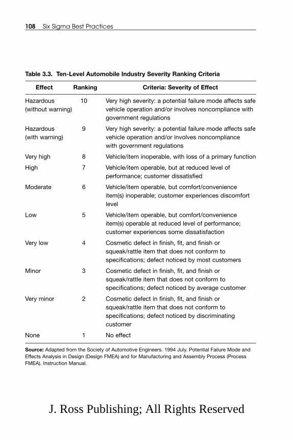
108 Six Sigma Best Practices
Table 3.3. Ten-Level Automobile Industry Severity Ranking Criteria
Effect Ranking Criteria: Severity of Effect
Hazardous 10 Very high severity: a potential failure mode affects safe (without warning) vehicle operation and/or involves noncompliance with
government regulations
Hazardous 9 Very high severity: a potential failure mode affects safe (with warning) vehicle operation and/or involves noncompliance
with government regulations
Very high 8 Vehicle/item inoperable, with loss of a primary function
High 7 Vehicle/item operable, but at reduced level of performance; customer dissatisfied
Moderate 6 Vehicle/item operable, but comfort/convenienceitem(s) inoperable; customer experiences discomfortlevel
Low 5 Vehicle/item operable, but comfort/convenienceitem(s) operable at reduced level of performance;customer experiences some dissatisfaction
Very low 4 Cosmetic defect in finish, fit, and finish orsqueak/rattle item that does not conform tospecifications; defect noticed by most customers
Minor 3 Cosmetic defect in finish, fit, and finish orsqueak/rattle item that does not conform tospecifications; defect noticed by average customer
Very minor 2 Cosmetic defect in finish, fit, and finish orsqueak/rattle item that does not conform tospecifications; defect noticed by discriminatingcustomer
None 1 No effect
Source: Adapted from the Society of Automotive Engineers. 1994 July. Potential Failure Mode andEffects Analysis in Design (Design FMEA) and for Manufacturing and Assembly Process (ProcessFMEA). Instruction Manual.
J. Ross Publishing; All Rights Reserved

priority than those having a lower RPN.6 The product of degree of severity (S),chances of occurrence, and detection ability (D) calculates the value of RPN aspresented in Table 3.5.
3.2.4.3 FMEA
FMEA is not as complicated as FMECA. The RPN is most commonly used forFMEA. The RPN is a product of three elements—severity ranking, occurrenceranking, and detection ranking. These elements are presented in Table 3.5. TheRPN value can range between 1 and 1000. The higher the RPN value, the higherthe risk of product/service failure. Commonly used steps in conducting FMEAinclude:
1. Develop a simple matrix spreadsheet with basic informationcolumns. (Table size will grow with product hierarchy.)
– Failure mode
– Cause of failure
– Effect of failure
– Severity ranking
– Occurrence ranking
– Detection ranking
– Risk priority
– Suggested improvement
Measure 109
Table 3.4. Four-Level Military/Government Severity Ranking Criteria
Category Explanation
I Catastrophic: a failure which can cause death or system loss(e.g., aircraft, tank, missile, ship)
II Critical: a failure which can cause severe injury, major propertydamage, or major system damage which will result in mission loss
III Marginal: a failure which may cause minor injury, minor propertydamage, or minor system damage which will result in delay orloss of availability or mission degradation
IV Minor: a failure not serious enough to cause injury, propertydamage, or system damage, but which will result in unscheduledmaintenance or repair
Source: Society of Automotive Engineers. 1993. Failure Mode, Effects and Criticality Analysis.Aerospace Recommended Practice, unpublished paper. Available athttp://www.sae.org/technical/standards/AIR4845.
J. Ross Publishing; All Rights Reserved

110 Six Sigma Best PracticesTa
ble
3.5
. G
uid
elin
es f
or
Ris
k P
rio
rity
Num
ber
(R
PN
)
Ran
king
Deg
ree
of
Sev
erit
yC
hanc
es o
f O
ccur
renc
e D
etec
tio
n A
bili
ty
10If
safe
sys
tem
fai
ls w
ithou
t Fa
ilure
ass
ured
(fro
m w
arra
nty
Cur
rent
con
trol
s p
ositi
vely
will
w
arni
ng t
hat
crea
tes
dan
ger
dat
a)no
t d
etec
t th
e p
oten
tial f
ailu
rean
d h
ostil
e ef
fect
on
cu
stom
er;
gove
rnm
ent
regu
latio
ns v
iola
tion
9If
safe
sys
tem
fai
ls w
ithou
t Fa
ilure
alm
ost
cert
ain
(from
Cur
rent
con
trol
s m
ost
pro
bab
lyw
arni
ng t
hat
crea
tes
dan
ger
war
rant
y d
ata
or s
igni
fican
tw
ill n
ot d
etec
t th
e p
oten
tial f
ailu
rean
d h
ostil
e ef
fect
on
cust
omer
; te
stin
g)go
vern
men
t re
gula
tions
vio
latio
n
8Ve
ry h
igh
leve
l of
dis
satis
fact
ion
Hig
h fa
ilure
rat
e (w
ithou
t an
yVe
ry h
ighl
y p
ossi
ble
tha
t th
ed
ue t
o lo
ss o
f fu
nctio
n, b
ut
sup
por
ting
doc
umen
tatio
n)p
oten
tial f
ailu
re w
ill n
ot b
ew
ithou
t ne
gativ
e im
pac
t on
det
ecte
d o
r p
reve
nted
bef
ore
safe
ty o
r go
vern
men
t re
gula
tions
re
achi
ng t
he n
ext
cust
omer
7H
igh
deg
ree
of c
usto
mer
R
elat
ivel
y hi
gh f
ailu
re r
ate
Hig
hly
pos
sib
le t
hat
the
dis
satis
fact
ion
due
to
(with
sup
por
ting
doc
umen
tatio
n)p
oten
tial f
ailu
re w
ill n
ot b
eco
mp
onen
t fa
ilure
with
out
det
ecte
d o
r p
reve
nted
bef
ore
com
ple
te lo
ss o
f fu
nctio
n,re
achi
ng t
he n
ext
cust
omer
but
pro
duc
tivity
imp
acte
d b
y
hi
gh s
crap
or
rew
ork
leve
ls
6 S
igni
fican
t co
mp
lain
ts a
bou
tM
oder
ate
failu
re r
ate
(with
out
Like
ly t
hat
pot
entia
l fai
lure
will
not
m
anuf
actu
ring,
ass
emb
ly,
orsu
pp
ortin
g d
ocum
enta
tion)
be
det
ecte
d o
r p
reve
nted
bef
ore
war
rant
yre
achi
ng n
ext
cust
omer
J. Ross Publishing; All Rights Reserved

Measure 111
5C
usto
mer
pro
duc
tivity
R
elat
ivel
y m
oder
ate
failu
reM
oder
ate
likel
ihoo
d t
hat
the
red
uced
by
cont
inue
dra
te (w
ithou
t su
pp
ortin
gp
oten
tial f
ailu
re w
ill r
each
deg
rad
atio
n of
effe
ct o
rd
ocum
enta
tion)
next
cus
tom
ercu
stom
er m
ade
unco
mfo
rtab
le
4C
usto
mer
dis
satis
fied
by
Occ
asio
nal f
ailu
res
Con
trol
s m
ay d
etec
t or
pre
vent
re
duc
ed p
erfo
rman
cep
oten
tial f
ailu
re f
rom
rea
chin
g ne
xt c
usto
mer
3C
usto
mer
exp
erie
nces
Low
fai
lure
rat
e (w
ithou
tLo
w li
kelih
ood
tha
t p
oten
tial
anno
yanc
e d
ue t
o sl
ight
su
pp
ortin
g d
ocum
enta
tion)
failu
re w
ill r
each
nex
t cu
stom
erd
egra
dat
ion
of p
erfo
rman
ceun
det
ecte
d
2C
usto
mer
exp
erie
nces
Low
fai
lure
rat
e (w
ithou
tA
lmos
t ce
rtai
n th
at p
oten
tial f
ailu
re
slig
ht a
nnoy
ance
sup
por
ting
doc
umen
tatio
n)w
ill b
e fo
und
or
pre
vent
ed b
efor
ere
achi
ng n
ext
cust
omer
1 C
usto
mer
will
not
not
ice
Rem
ote
likel
ihoo
d o
f C
erta
in t
hat
pot
entia
l ad
vers
e ef
fect
or
effe
ct n
ot s
igni
fican
t oc
curr
ence
failu
re w
ill b
e fo
und
or
pre
vent
ed
bef
ore
reac
hing
nex
t cu
stom
er
So
urce
: Jur
an,
J.M
. 20
02.
Jura
n In
stitu
te’s
Tra
nsac
tiona
l Bre
akth
roug
h S
trat
egy.
Sou
thb
ury,
CT:
Jur
an In
stitu
te.
Cha
pte
r 3
(stu
den
t m
ater
ial f
rom
Bla
ckB
elt
cert
ifica
tion
trai
ning
cla
ss).
J. Ross Publishing; All Rights Reserved

2. Obtain ranking data from Table 3.5. It is important to note that thefailure occurrence ranking will depend upon who is using the prod-uct, e.g., a hammer being used by a carpenter vs. the hammer beingused by an orthopedic surgeon. The team should choose valuesbased on product history, similar models, actual occurrence data(generally from customers), process capability studies,simulation/mathematical modeling, and testing.
3. Identify the cause of failure based on past experience, cause-and-effect analysis, or from some other source. If there is more than onepotential cause for failure for each mode, list all of these causesdirectly under each other on a separate line. Analyze how each fail-ure will affect customers, the overall product, or the system.
4. From Table 3.5, evaluate the degree of severity for each failure andchoose an appropriate ranking from the table.
5. Analyze and choose the detection ranking value from Table 3.5. Takeadvantage of historical data if available.
6. Calculate the RPN factor by multiplying all three of these factors.The cause that receives the highest score is the one that requires themost attention from the team so that a method(s) to correct the fail-ures can be identified.
7. The best time to apply the FMEA tool is when the product/service isin design stage. Generally, design actions are not performed for eachmode that might fail, but only for the “critical” modes. Take advan-tage of Pareto Analysis to rank the “risk priority.” Once the teamselects the modes which require further attention, design actionswill reduce the level of failure rate that is acceptable to the team.
8. Validation of each solution is important. Validation will ensure thatthe design action will reduce potential failure to an acceptable level.It is important to design a plan to validate the effectiveness of eachaction and revise the design as needed.
The FMEA process is explained in Example 3.4. See Section 3.2.4.4 for a dis-cussion of the modified FMEA process.
Example 3.4: The FMEA Process
The product is New Employee Business Card. Business cards are sent to each newemployee after he/she joins the company. The component being evaluated isBusiness Cards. The failure mode is Business Cards Are Printed Incorrectly, with thefollowing elements:
• Employee’s name is incorrectly spelled.
112 Six Sigma Best Practices
J. Ross Publishing; All Rights Reserved

• The office telephone number is incorrect.
• Employee’s e-mail address is incorrect.
Possible causes of failure are numerous, e.g.,
• Request form—Employee’s name on request form is in cursive writing.
• Data entry error—Historical data show approximately 27 errors per10,000 telephone number data entries.
• Employee’s e-mail address—Employee’s first name dot last name@company name dot com is in cursive writing.
Historical data entry error statistics for some industries is ranked and pre-sented in Table 3.6A. The FMEA information is presented in Table 3.6B.
The combined highest RPN factor is 216 for Data entry error. Such an erroris likely to cause a complaint; yet it has some chance of detection before the erroraffects the customer. Therefore, to minimize this risk, a special review step isrequired in the software.
3.2.4.4 Modified FMEA
The modified FMEA process will be discussed utilizing an example from a man-ufacturing area. Modified FMEA is used to determine failures that are occurringin a manufacturing facility and to determine their impact and frequencies.Discuss a hydraulic pump in a tractor with the following data:
• Failure event—Failure of pump
• Failure mode—Bearing failures
• Frequency—9 failures per year
• Impact—$3,000 per failure
• Total loss—$27,000 per year
Measure 113
Table 3.6A. Historical Error Statistics
Ranking 10 9 8 7 6 5 4 3 2 1
Error Frequency per 10,000 Data Entries
Office and 45 40 35 30 27 22 17 10 6 <2printingindustry
Banking 45 38 32 27 22 18 14 10 6 <2industry
J. Ross Publishing; All Rights Reserved

114 Six Sigma Best Practices
Tab
le 3
.6B
. FM
EA
Inf
orm
atio
n fo
r E
mp
loye
es’ B
usin
ess
Car
ds
Mo
de
of
Cau
se o
fE
ffec
t o
fD
egre
e o
fC
hanc
es o
fD
etec
tio
nR
PN
Failu
reFa
ilure
Fa
ilure
Sev
erit
yO
ccur
renc
eA
bili
ty(1
–100
0)P
rop
ose
d1
23
45
64�
5�6
Imp
rove
men
t
Bus
ines
sE
mp
loye
eM
ust
64
819
2W
rite
nam
eca
rds
nam
ere
prin
tin
cap
ital
prin
ted
writ
ten
inca
rds
lett
ers
inco
rrec
tlycu
rsiv
e
Dat
a en
try
66
621
6H
ave
revi
ewer
ror
step
in s
oftw
are
e-m
ail
64
819
2W
rite
e-m
ail
add
ress
ad
dre
ss in
writ
ten
in c
ursi
ve
cap
ital l
ette
rs
J. Ross Publishing; All Rights Reserved
If a similar type of calculation were performed on every failure, the resultswould be astounding, but they would not be cost-effective. Working on every fail-ure event is not practical. Therefore, determine the most significant failure eventsutilizing the concept of Vilfredo Pareto, the well-known Italian economist. Theconcept of the 80/20 rule is that 80% of failure losses may be coming from only20% of the parts/assembly. This means a root cause failure analysis (RCFA) doesnot have to be done for every failure event, only for the ones that are the mostimportant. The analysis process can be divided into steps:
1. Complete preparatory work.
2. Collect failure and related data.
3. Summarize information.
4. Analyze information for losses.
5. Determine significant elements.
6. Validate results.
7. Develop a report with recommendations.
Step 1. Complete Preparatory WorkIt is important to do some preliminary preparatory work before starting anyanalysis. A Six Sigma mission statement has already defined the issue for thisanalysis, i.e., a hydraulic pump. Cover the following elements in Step 1:
• Develop a failure definition.
• Draw a contact flow chart.
• Calculate the gap analysis.
• Develop a preliminary interview schedule.
Developing a failure definition seems trivial, but it is an essential step in theanalysis. If a large group of people (say 50) were asked to define failure, therewould probably be 50 different definitions, which would make the analysis far toobroad and difficult to complete. Focus on the things that are most important tosatisfy customers and the business. For instance, if the tractor stays operational,this situation is good for the customer, but it is critical for the business; therefore,center the failure definition on keeping the tractor operational. Commonly usedfailure definitions include:
• Failure is a loss of equipment availability.
• Failure is a deviation from the status quo.
• Failure is any loss that interrupts the continuity of operation/production.
• Failure is not meeting expectations.
Measure 115
J. Ross Publishing; All Rights Reserved

There are no perfect failure definitions. Because the product is analyzed basedon the defined definition of failure, a precise failure definition is not important.Consider some simple rules when developing a failure definition:
• It must be concise and easily understandable; otherwise the failuredefinition will leave excessive opportunities for interpretation.
• It should not have to be interpreted.
• It must address only one topic.
• It should be approved and signed (if possible) by someone withauthority.
Next, draw a contact flow chart. Developing a contact flow diagram will allowthe system to be broken down into smaller, more manageable subsystems. Therule for a contact flow chart is to map all the process units that come into contactwith the product.
Then calculate the gap analysis, which helps uncover the disparity betweenwhat the company is producing now and what its potential production is. Applygap analysis to the hydraulic pump to get some indication of the potential oppor-tunity in the manufacturing facility. For instance, the company is producing15,000 hydraulic pumps per year; however, the potential is 25,000 per year. Thecompany has a gap of 10,000 hydraulic pumps per year.
Developing a preliminary interview schedule is the final step in the preparationstage. Design a preliminary interview sheet and a schedule for interviewing peo-ple. This will lead to data collection.
Step 2. Collect Failure and Related DataThere are two ways to collect failure and related data for this analysis:
• From a data file maintained in the system
• By interviewing people who are closest to the work
Although each data source has its advantages, interviewing people is proba-bly better than obtaining information from the data file because informationfrom an interview is “straight from the source.” If there is enough confidence inthe company data files, they can be used to validate the interviews.
It is best to interview the people who are closest to the work, e.g., machineoperators, mechanics, assembly employees, and test employees. Talk to supervi-sors and managers, but certainly not to the same extent as with mechanics, oper-ators, and assembly employees.
Explain the process to the interviewees, ask the questions, and note the infor-mation on a log sheet. The interviewing task can be quite an experience.
116 Six Sigma Best Practices
J. Ross Publishing; All Rights Reserved

Interviewing tends to be more of an art than a science. Tips for conducting aninterview include:
• Take care to ask exactly the same question to each of the interviewees.This helps eliminate the possibility of having different answersdepending on interpretation of the question.
• Expand on the questions if further clarification is required.
• Ensure that participants know what is being worked on and the pur-pose of the interview. If the purpose and process are not clearlyunderstood, the interview process might appear to the interviewees tobe more like an interrogation than an interview.
• Allow the interviewees to see that their answers are written on theinterview form. Never use tape/video recording equipment in aninterview session because it tends to make people uncomfortable andless likely to provide information.
• Never argue with an interviewee. If an interviewer does not agree withthe person, it is best to accept what he/she is saying at face value andcheck it against the information from other interviews.
• Always be aware of interviewees’ names. People love to hear their ownnames. Write interviewees’ names in a prominent place for easy refer-ence.
• Develop a strategy to draw out quiet participants. Many quiet peoplein the workforce have a wealth of data, but are not comfortable withproviding it to others.
• Be aware of body language. Although books have been written on thisscience, being an expert in reading body language is not required. Yet,it is important to recognize that significant human communication isprovided through body language.
• Note extraordinary contributors. In any set of interviews, some peo-ple are able to contribute more information to the process than oth-ers. Make a list of extraordinary contributors so that they can provideassistance later in the analysis.
• Use the failure (defect) definition and flow chart to keep intervieweeson track if they begin to wander from the subject.
Step 3. Summarize InformationOnce the information is collected, the next activity is to analyze the data for thepossibility of redundant entries. Convert frequencies from the interviewees’ meas-urement units into occurrences per year (e.g., 1 per week translates to 52 times peryear).
Measure 117
J. Ross Publishing; All Rights Reserved

Input this information into an electronic spreadsheet. Once the informationis input, sort the raw data first by subsystem and then by failure event. This willprovide a closer look at the events that are redundant.
The hydraulic pump example data are summarized in Table 3.7. The data sug-gest that the first three items are the same because all impact the bearings andhave fairly consistent frequencies and impacts. The last three items are also relatedto bearings, but they go one step beyond the others. The hydraulic pump not onlylost a bearing, but it also has a failed seal, a clogged filter, and a cracked shaft,which indicates three separate modes of failure. A summary of the information ispresented in Table 3.8.
Step 4. Analyze Information for LossesOnce the product and time losses have been identified, a simple calculation deter-mines total loss for each event in the analysis:
Total loss per year = Frequency � loss per occurrence (impact)
The example data are presented in Table 3.9.
It is important to ensure that loss is communicated in the most appropriateunits. In Table 3.9, losses are shown in hours of downtime, which might not meanmuch to some people. It might be more advantageous to convert the numberfrom hours per year to dollars per year because everyone can relate to dollars.
Step 5. Determine Significant ElementsAs indicated earlier, utilize the 80/20 rule, in which 80% of the losses are represen-tative of 20% of the issues (failures). The concept is visible in the Table 3.9 data aswell. The total loss is 442 hours. Bearing failure accounts for 360 loss hours, whichis equal to 81% of the total loss hours. Therefore, bearing failure is a significantelement. Now, instead of doing RCFA (root cause failure analysis) on everything,RCFA is only done on bearing failure.
Step 6. Validate ResultsValidation of collected data at this point is important. Gap analysis (compareinterview data with the system failure data file) can be used to ensure that all ofthese events add up to ±10% of the gap. If collected data end up being less, someimportant failure events have probably been omitted from the listing. If there ismore than the gap, then results have probably not been summarized well enough.There may be some redundancies on the list. Sometimes many small events (e.g.,a few minutes of repair) are never even recorded in the system failure data file.
118 Six Sigma Best Practices
J. Ross Publishing; All Rights Reserved

Measure 119
Table 3.7. Summary of the Interview Data—Hydraulic Pump Failure
ImpactSubsystem Failure Event Failure Mode Frequency (Lost Time)
Load lift Recirculation pump Bearing pails 1 per month 1 shiftLoad lift Recirculation pump Oil contamination 1 per month 10 hoursLoad lift Recirculation pump Bearing freeze 1 per month 10 hoursLoad lift Recirculation pump Seal fails 1 per 2 months 1 shiftLoad lift Recirculation pump Shaft cracked 1 per year 10 hoursLoad lift Recirculation pump Filter clogged 1 per month 2 hours
Table 3.8. Analyzed and Summarized Data
ImpactSubsystem Failure Event Failure Mode Frequency (Lost Time)
Load lift Recirculation pump Bearing problem 36 per year 10 hoursLoad lift Recirculation pump Seal fails 6 per year 8 hoursLoad lift Recirculation pump Filter clogged 12 per year 2 hoursLoad lift Recirculation pump Shaft cracked 1 per year 10 hours
Table 3.9. Yearly Product Loss Data
Total LostProduction
Subsystem Failure Event Failure Mode Frequency Impact (Hours/Year)
Load lift Recirculation pump Bearing fails 12 per year 10 hours 360 hoursLoad lift Recirculation pump Seal fails 6 per year 8 hours 48 hoursLoad lift Recirculation pump Filter clogged 12 per year 2 hours 24 hoursLoad lift Recirculation pump Shaft cracked 1 per year 10 hours 10 hours
Total Time Loss = 442 production hours
J. Ross Publishing; All Rights Reserved

A second validation method is to have a group of experienced people fromthe manufacturing facility to review the findings. This will help ensure that thefindings are not too far off base.
Step 7. Develop a Report with RecommendationsCommunicating the findings to all interested parties is important. The reportshould include:
• An explanation of the analysis technique
• The failure definition that was utilized
• The contact flow diagram that was utilized
• Graphically displayed results, as well as the supporting spreadsheetlists
• Recommendations of failures that are candidates for RCFA
• A listing of everyone involved in the analysis, including all of interviewees
Communicate results of the analysis to the interviewees, so that all partici-pants will have a sense of accomplishment and ownership. Most organizationscollect significant amounts of data, but the question is, “Will this data provide theinformation that will be needed for the project?” If the collected data does notprovide the necessary information, develop a data collection plan. Section 3.3 willdiscuss the data collection plan, but before proceeding to Section 3.3, considerExercises 3.2 and 3.3.
Exercise 3.2: Process Improvement
Using information in Example 3.1 as a basis:
• Develop a detailed process map.
• Develop a list of potential improvements. The architect has designeda fancy house. The estimated cost for the house is very high. The cus-tomer’s main complaint is the expensive house design. Use processmap analysis and the cause-and-effect diagram to develop a list ofpotential improvements.
• Prioritize the improvement list.
Exercise 3.3: A FMEA Analysis
The product to be considered is new checks for a new joint money marketaccount. The component being evaluated is New Checks. The new checks will bemailed to the customer, a married couple. This new account is a joint account inwhich both spouses have check-writing privileges and both authorizing signatures
120 Six Sigma Best Practices
J. Ross Publishing; All Rights Reserved

are required when a check is issued from the joint money market account. Thenew checks are printed incorrectly:
• Incorrectly spelled customer names
• Only one line for authorizing signatures
• Incorrect account number
Possible causes of the errors are numerous. One cause could be a data entryerror. Historical data show approximately 27 errors in 10,000 account numberdata entries. Such an error is likely to cause a complaint, yet the chance of detec-tion before this error affects a customer is low. Ranking of historical data entryerror statistics for sample industries is presented in Table 3.6A.
Perform a FMEA analysis and make recommendations.
3.3 DATA COLLECTION PLAN
In the measurement phase, Six Sigma project leaders should develop a sound datacollection plan. Data are nothing but facts. Generally, most organizations havevast stores of information about their operation, but when a Six Sigma teambegins working on a project, they often find that the information they need doesnot exist. Sometimes the project team’s collected data does not contain the infor-mation that the project leaders are looking for. Therefore, project leaders shouldthink about:
• What information is wanted and how will it be obtained?
• What information collection tool should be used and where can theinformation be found?
• How will the information be utilized to achieve conclusions?
There is no need to utilize a sophisticated statistical sampling plan if the col-lected information does not answer a question or if users do not care about thebenefit.
Like any planning process, some iteration may be required to complete thedesign of a good data-collection system. Data collection is very similar to a pro-duction process and, like any process, critical is first understanding the processand then improving the process.
Note: Significant work has been done on the data collection process.Information is available in the literature.
Several crucial steps need addressing to ensure that the data collection processand measurement systems are stable and reliable. Once these steps have been
Measure 121
J. Ross Publishing; All Rights Reserved

incorporated into the data collection plan, the probability that the collected dataand the measurement system will meet project requirements will increase. A datacollection plan can be divided into six data collection steps:
1. Define goals and objective.
2. Develop good questions.
3. Define operational definitions and methodology.
4. Ensure repeatability, reproducibility, accuracy, and stability.
5. Define the data collection process.
6. Review data collection.
Step 1. Define Goals and ObjectivesIdentify the purpose of data collection and how it will support the project objec-tives. A good data collection plan should include:
• A precise and focused project description
• The specific data needed to support the project
• The supporting reasons for collecting the data
• Insight information that the data might provide about the project andhow it would help the project team
• How data will be utilized once it has been collected
Understanding these elements will facilitate accurate and efficient data collec-tion by the team. For example, a project’s goal is to reduce printer assembly andtest time. As the project team develops a process flow chart and identifies theactivities as value added, non-value added, and waste, the next step will be toeither find the historical data or, if historical data are not available, to collect thedata. Analysis of the collected data will provide team members with a betterunderstanding of the distribution of assembly and test cycle time into value-added, non-value added, and waste. To reduce cycle time, the team would try tominimize non-value added activities and eliminate waste activities. Some com-monly utilized non-value added activities are material movement, material stor-age, and data entry; waste activities are waiting for parts, assembling wrong parts,etc. Therefore, defining goals and objectives in a data collection plan is a criticalstep. Next is developing good questions about the type of information that shouldbe collected.
Step 2. Develop Good QuestionsAsking the right questions is important in any successful data collection process.Questions should be prioritized based on the expected information as it relates to
122 Six Sigma Best Practices
J. Ross Publishing; All Rights Reserved

project requirements. Higher-priority questions should provide pertinent infor-mation for the project.
Higher-priority questions clearly indicate the data that need to be collected.The initial effort invested in formulating specific, well-focused questions is morelikely to provide a better return and also reduce the efforts required to design,implement, and analyze the information from the data collection system.Particularly beneficial to the project is input from a person(s) who understandsan area and the project requirements very well. For example, the answers fromquestions 1b and 2b are more informative than the answers from questions 1a and2a:
1a. Are Customer Support groups handling Customer Issue Reports ina timely manner?
or
1b. When the Field Service Organization receives a Customer IssueReport from the Customer Support group, how much time is left forthe repair technician to resolve the problem relative to the servicetime that Customer Support representative promised the customer?
2a. Are branch offices making errors in the new account applicationsthat waste resources in the main office operation?
or
2b. What percent of new-account applications from branch offices arereceived at the main office that require follow-up with a branchoffice representative or a new-account customer because informa-tion is missing, conflicting, or incorrect on the application form?
Also advisable is thinking about data analysis and presentation before begin-ning any data collection. Sometimes, a team has to repeat a data collection studyor, even worse, make a decision based on an incomplete analysis because theteam’s data are not complete enough to support the level of analysis the teamwants to perform.
Step 3. Define Operational Definitions and MethodologyTo facilitate measurement, a Six Sigma team should clearly define and decide:
• What and how data will be collected
• What will be evaluated and how a numerical value will be assigned
The team should consult customers to see if they are already collecting thesame or similar data. If so, comparisons should be made and the best practicesshould be shared. The team should also define the additional scope:
Measure 123
J. Ross Publishing; All Rights Reserved

• How many observations will be needed?
• What will be the time interval for subsequent data collection?
• Will past, present, and future data be collected?
• What methodologies will be employed to record all the data?
Note: If the team wishes to include historical data as part of the study, paycareful attention to how reliable the data and its source have been and if continu-ing to use such data is advisable. Suspect data should be discarded.
When all the data on a population are collected, this data are often referred toas a census. A portion or subset of the total data collection process is known assampling. There are three key sampling advantages:
• The objective is to predict or draw conclusions about the populationusing the sample.
• Often collecting all the data is impractical or too costly.
• Sometimes data collection is a destructive process.
Sampling data must have qualities that meet certain criteria:
• Unbiased
• Random
• Representative of population
UnbiasedThe project team must inspect the data before using in the project. If a sampleappears to be different from the population or the process due to the presence orinfluence of any factor, the sample is known as a biased sample. As data are col-lected, biases may occur:
• Estimation bias—If repeated random samples from a given popula-tion produce a statistic with a mean or expected value that differsfrom the target to be estimated, it is defined as estimation bias (illus-trated in Figure 3.7). Conversely, a sample statistic on the average andacross many samples that takes on a value equal to the populationparameter that is to be estimated is called an unbiased estimator. Forexample,
Let:T = True value of population parameter or the target valueE = Sample estimatorμE = Mean of sampling distribution
124 Six Sigma Best Practices
J. Ross Publishing; All Rights Reserved

Then:μE – T = Sample bias
Bias was introduced when the data were collected without regard to key ele-ments that could influence the population or process. A sample is considered tobe representative of the population only when it is bias-free.
• Exclusion bias—Service call response time is defined as “the clockstarts once the message is read/listened to and the clock stops whenthe service person reaches the customer site.” If any portion of thisservice call response time is excluded from the analysis, the analysis isdefined as exclusion-biased.
• Inclusion bias—The service time clock starts when the service techni-cian reaches the customer site and the clock stops when the servicetechnician completes the job and leaves the customer site. If the serv-ice technician’s travel time from the office to the customer site isincluded in the data, the data is inclusion-biased.
Accuracy and precision. Collect several measurements on a single unit ofproduct and then compute the mean. The accuracy of the collected data would
Measure 125
E
E
f(E)
f(E)
T = μ
T
Bias
E
μE
Figure 3.7. Unbiased vs. Biased Estimator
J. Ross Publishing; All Rights Reserved

depend on the difference between the sample mean and the true mean. The spreadof values around the mean is called the precision, or repeatability, of the system.Usually accuracy and precision are thought of in reference to meters and gauges,but it is important to note that these concepts also apply to human sensing. Forexample, if four product-checking inspectors work on a manufacturing floor andexamine the same product separately, a high probability exists that each inspectormay find a different number of errors—a result known as lack of precision.Furthermore, all of the inspectors may fail to identify a specific error—a resultidentified as lack of accuracy. Training classes for product checkers and inspectorsand ongoing audits are the techniques for ensuring accurate and precise data.
Another way of looking at sample data accuracy is with a scenario. For exam-ple, a team wants to establish the accuracy of its process to measure defects in pur-chase orders. First, the team collects a “standard group” of purchase orders. Thenthis team has an “expert group” establish the type and number of defects in thecollected group of purchase orders. Next, a “normal group” (regular employeesworking in the purchasing department) checks the standard group of purchaseorders. Differences between what is found in the standard group of purchaseorders by the normal group and what the known defect level is as established bythe expert group represent the inaccuracy or bias of the measurement process.
• Missing data bias—Missing data can bias conclusions.
• Professional bias—Failure to follow an established data collectionprocess is the most common professional bias.
RandomRandomness in the collected data helps to avoid biases. Data should be collectedin no predetermined order, and each element should have an equal probability ofbeing selected for measurement:
• Time specific
• Order of data collection
• Data collector
Representative of PopulationCollected sample data should accurately reflect the population or process.Representative sampling would help the project team to avoid biases, specificallyin the proposed process or the population under investigation. If the populationis small, there is always the option of not taking samples, but instead to use theoption of collecting data from the entire population. This option might providethe most accurate measure of the average (mean) value, but for logistic and/orcost reasons, it might not be practical.
126 Six Sigma Best Practices
J. Ross Publishing; All Rights Reserved

A commonly used approach is to obtain a representative sample and estimatethe parameters based on the sample. This approach costs less, but does not pro-vide as much accuracy as would be obtained from the population.
If the team knows the degree of accuracy about the sample mean in relationto population mean, then the team assigns the usefulness value to the sample datain the decision-making process—known as the confidence interval. For example,when estimating the average service time from samples, the team may obtain a95% confidence interval for the average of 2.5 to 3.5 hours, which means that ifthe team takes repeated samples from the population, 95 out of 100 times theteam would expect the sample average to be between 2.5 and 3.5 hours. The sta-tistical theory that supports the confidence interval is known as the Central LimitTheorem. (See the discussion in Section 3.7, Probabilistic Data Distribution.)
Sample size and sampling frequency are important issues in data collection.A rule of thumb in sample size is that between 25 to 45 data points are considereda good sample. (See Section 3.6, Determining Sample Size.) Sampling frequencydepends on the data collection objective. For example, if the data collection objec-tive is to understand hour-to-hour variation, samples would need to be taken atleast every hour, preferably more than one data point every hour.
Step 4. Ensure Repeatability, Reproducibility, Accuracy, and StabilityThe project team must recognize that over any length of time, and if data are notconforming to the repeatability, reproducibility, accuracy, and stability factors,unreliable data may be collected. A good practice is testing, perhaps on a smallscale, how data collection and measurement should proceed. Upon simulation,the possible factors and what could be done to mitigate the effects of these factorsor to eliminate the factors altogether should become apparent. Next is a shortdescription of each factor.
RepeatabilityThe data being collected (measured) should be repeatable. In the same setting, anoperator/collector should be able to reach essentially the same outcome multipletimes for a defined process/product when using the same equipment. For exam-ple, an operator is producing a rough-turned steel shaft on a turning machine.Production time takes 5 minutes. If the same setting is used to produce a secondshaft, the production time should be very close to 5 minutes.
ReproducibilityAll data collectors who are measuring the same items with the same equipmentshould reach essentially the same outcomes. For example, consider a packagingoperation. A packaging operator is wrapping each book individually, then pack-ing five books in a box, and then sealing and labeling the box. A member of thedata collection team timing the packaging cycle time recorded the time as 6 min-
Measure 127
J. Ross Publishing; All Rights Reserved

utes. If another person from the data collection team collects the packaging cycletime data, then he/she should measure almost the same time.
AccuracyThe degree to which the measurement system is accurate would generally be thedifference between an observed average measurement and the associated knownstandard value. For example, if the inches on a ruler were divided into eight (8)parts, the smallest measurement on the ruler would be an eighth (1/8) of an inch.If this ruler were used to measure the length of a bar, then the smallest fractionvalue that could represent the difference between the observed and the standardvalue measured would be an eighth of an inch (1/8 inch).
StabilityThe degree to which the measurement system is stable is generally expressed bythe variation resulting from the same data collector measuring the same item withthe same equipment over an extended period. For example, in the heat-treatingprocess of a shaft, if smaller were the variation in the processing time and heat-treated shaft quality, then higher would be the system stability.
Step 5. Define Data Collection ProcessData collection steps 1 through 4 assist a team in defining/identifying their dataspecifications and requirements. The data specifications and requirements willlead to defining the data collection process. Once the data collection process hasbeen defined and developed, follow-through from start to finish of the processwill ensure that the plan is being executed consistently and accurately.
The project leader has the responsibility of communicating what is to be col-lected and the rationale behind it to all data collectors and participants.Additionally, the team leader should review all applicable definitions, procedures,and guidelines and confirm with each team member that there is universal agree-ment among the team members. Follow-up could be some form of training or ademonstration of the data collection process as defined in the plan.
Oversight by the team leader during the data collection process is preferred.Oversight allows participants to know if the plan is being followed properly orimproperly. Failure to oversee the data collection process at the early stages mightmean that a later-course correction will be required. Much of the data collectionand/or measurement efforts would be wasted.
It is important to realize that data are being collected for a Six Sigma proj-ect—the project has already been recognized as having a serious problem.Therefore, there is a high probability that the process has numerous rework loopsand complex flow patterns that have been added over the years in an effort to keepthe process working despite its problems. This type of process complexity makesdata collection difficult. For example, an inserter manufacturing company discov-
128 Six Sigma Best Practices
J. Ross Publishing; All Rights Reserved

ered that their customer order booking process could follow as many as six differ-ent paths due to changes in system configuration, customer job requirements, andpoor communication between customers and manufacturer’s technical group.Data collectors must identify the exact process as they collect data in this type ofprocess.
Six Sigma team leaders should think carefully about the possibility of biasbefore asking a person in the process area to collect data. If bias is a possibility, theteam leader should select an independent observer to collect information (data).Specific examples include:
• If a Six Sigma team member is collecting data, a probability of processalteration exists. This alteration is nothing more than a minor incon-venience to the process team, but this team member may introducenew conditions into the process, which fundamentally change theprocess performance and can result in biased data or a misrepresenta-tion of the actual process.
• Although it may be tempting and convenient to use supervisors ormanagers as data collectors, resist this temptation. Sometimes, mem-bers of management cannot resist the temptation to draw their ownconclusions and begin tampering with the process during the datacollection effort. Additionally, if employees learn that their manager iscollecting data, they might alter the process during the study period.
In either case, the result can be biased data.
• Commonly project team members serve as data collectors, a practicewhich can also produce biased data. For example, if a team memberhas some advanced theory or hypothesis about the cause of the prob-lem, and this team member has been assigned to collect data, he/shemay unintentionally disregard observations that are not consistentwith his/her theory or hypothesis or he/she may inadvertently tamperwith the process by discussing suggestions for changes with theprocess resource while collecting data. Assignment of the persons whowill perform the data collection task is critical.
An “independent observer” can also be a technological tool rather than a per-son. Automated data collection, using self-recording test equipment, video cam-eras, or computers with verifications and crosschecking, can be a very effectiveway to collect accurate, unbiased information without disrupting the naturalprocess. Also important is ensuring that the automated data collection device isobserving the complete picture.
Another way to avoid bias is to compile existing data for another project(process) and use that data for the selected project. For example, if the team is
Measure 129
J. Ross Publishing; All Rights Reserved

interested in service response time, it might analyze a service request message fordate and time, and then compare that information with the service technician’slog-in date and time at the customer site. There would definitely be less potentialfor bias in this data than there would be in a special study request to the ServiceGroup to collect data.
Once the team has defined the questions, the type of data needed, the datacollection points in the process, and the data collectors, the Six Sigma team is nowready to design the data collection form. If data are to be collected on a computer,the team must design the data-reporting screen so that all pertinent data are col-lected. For example, suppose a team wants to collect start and end times on amachine for an operation. If two machines are available and the operator has theoption of selecting either machine, then the data reporting screen must displayboth machines on the screen so the operator can provide the start and end timesfor the actual machine used for the operation. Basic requirements in a data collec-tion form include:
• Utilize the concept of KISS (Keep It Simple, Stupid). When people arestruggling or are simply too busy trying to deal with a problem, thelast thing on their mind is collecting data for a team’s project. If theteam designs the form and keeps the data collector’s needs in mind,people involved in recording the data will be more willing to acceptthe task.
• Design the form to reduce the possibility of errors in recording orinterpreting the data. Provide options when possible, e.g., a checklist.
• Provide pictures, sketches, and examples. “Clues” can help ensuremore consistent and reliable data.
• Design the form to also collect additional information for futureanalysis, reference, and traceability, e.g., reference information such asdate, time, shift, place (location), equipment, operator, material, etc.
• Design the form to be as self-explanatory as possible, with minimuminstructions.
• Provide a professional looking data collection form or data collectioncomputer screen, e.g., a handmade form with handwritten informa-tion is difficult to read and understand.
Once the information collection process has started, next is to audit/monitorthe process.
Step 6. Review Data CollectionReferring to the questions of “Are the data collection and measurement systemsreproducible, repeatable, accurate, and stable?” and “Are the results (data and
130 Six Sigma Best Practices
J. Ross Publishing; All Rights Reserved
measurement) reasonable?” and “Do the results meet the criteria?” is important.For example, the project team should audit the data-collection effort at randomby reviewing the data collection process and reviewing the data collected forms.There is no reason to wait until all data have been collected. The nature, degree,and the formality of such audits will vary according to the complexity of the project.
If the results do not meet the criteria, then the team leader should determinewhere breakdowns exist and what to do with data and/or measurements that aresuspect. Review the operational definitions and methodology with the partici-pants (team members) and try to clear up any misunderstandings or misinterpre-tations that might have caused the breakdowns.
Once the data have been collected, they must be presented. Section 3.4 willdiscuss the Data Presentation Plan. Before moving on, consider Exercise 3.4.
Exercise 3.4: A Data Collection Plan
Using information in Example 3.1 as a basis:
1. Develop a data collection plan for an architect’s house design project.
2. Identify questions to be answered from the collected data.
3. Justify the sampling data plan.
4. Identify data collection points.
5. Develop a data collection form(s).
6. Develop a data audit and validation plan.
Important considerations:
• Ensure that the data collectors are unbiased.
• Provide appropriate instructions with the data collection form(s).
• Provide basic training in data collection if necessary.
• Provide oversight during the data collection process.
3.4 DATA PRESENTATION PLAN
Data present information about a product or process. The data may be qualitativeor quantitative. In any project/process, effective presentation of the data is asimportant as the collection of the data. Weeding out irrelevant information andconveying all relevant information accurately and unambiguously are also impor-tant. Because data may support or reject project objectives, data become a verycritical part of any project or process.
Numerous data presentation techniques are available to describe data. Somecommonly used techniques will be described:
Measure 131
J. Ross Publishing; All Rights Reserved
• Tables, histograms, and box plots describe both the central tendencyand the distribution of data.
• Bar graphs and stacked bar graphs compare information from differ-ent sources.
• Pie charts proportionate the distribution relationship in the data(information).
• Line graphs, control charts, and run charts describe data (informa-tion) changes over time.
• Mean, median, and mode describe the central tendency of data.
• Range, variance, and standard deviation describe data distribution.
As a project team analyzes the data, the team must determine which dataproperties that support project issues/problems are dominant in the collected/his-torical data:
• If the team is looking for “What is the central tendency of the data?”and/or “Where do the values tend to occur?” then the team shouldanalyze the data for mean, median, and mode.
• If data distribution (dispersion) is the team’s interest, then the teamshould analyze the data for range, variance, and standard deviationand try to summarize the information in tables, histograms, and boxplots.
• If the team is interested in knowing the data variation over time andif there is any trend over time, the team should summarize the data inline graphs, control charts, and run charts.
• If the team is interested in the proportionate distribution of data, theteam should to summarize data in a pie chart.
• If the team is interested in comparing data from different sources, theteam should develop bar graphs and stacked bar graphs.
These data presentation techniques will now be described with examples.
Note: Several software tools such as the MINITAB software package are alsoavailable for data presentation and statistical analysis. The application ofMINITAB will be briefly discussed in Section 3.5.
132 Six Sigma Best Practices
J. Ross Publishing; All Rights Reserved

3.4.1 Tables, Histograms, and Box Plots
TablesConstructing a good statistical table is an art that requires a great deal moreunderstanding and participation than simply presenting data in rows andcolumns. Specific table attributes are necessary to develop tables and to obtain themost useful information to support the project/process (see Tables 3.10 and 3.11for examples):
Ordered array. Listing data in a table in ascending or descending magnitudeis a major improvement. Most users are not interested in the detail contained inthe table or they prefer considerable condensation of the data.
Classes. To best serve the goal of clarity, personal judgment is used to deter-mine how many collectively exhaustive and mutually exclusive groupings (classes)of data should be made. An example will explain the concept of grouping:
• Grouping type: Qualitative, e.g., the type of business (partnership,proprietorship, or corporation), which is then subdivided into small,medium, and large
• Grouping type: Quantitative, e.g., the number of personal computers(PCs) owned by households (households own 0 PC, 1 PCs, 2 PCs,etc.)
• Grouping type: Continuous quantitative, e.g., gallons of gasoline pro-duced in the oil refinery industry
In the case of quantitative data, determining class is also considered desirable:approximate class width = (large value – smallest value in data set)/desired num-ber of classes.
Absolute class frequency. The absolute number of observations that falls intoa given category is defined as the absolute class frequency.
Absolute frequency distribution. The tabular summary of a data set showingthe absolute class frequencies in each of the classes is known as the data set’sabsolute frequency distribution.
Relative class frequency. Relative class frequency is a fraction or proportionof all observations that fall into various classes, i.e., the ratio of the number ofobservations in a particular class to the total number of observations collected.
Relative frequency distribution. The tabular summary of a data set present-ing the relative class frequencies in each of the classes is known as the data set’srelative frequency distribution.
Cumulative class frequency. A cumulative class frequency is the sum of the(absolute or relative) class frequencies for all classes in question (project study)for the given quantitative data. Accordingly, a cumulative frequency distribution isa tabular summary of a data set showing for each of several classes the absolute
Measure 133
J. Ross Publishing; All Rights Reserved
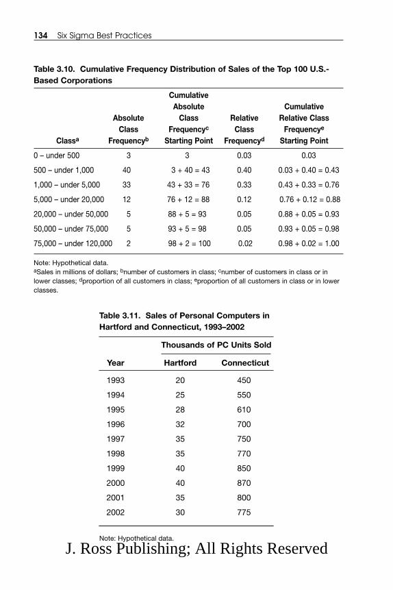
134 Six Sigma Best Practices
Table 3.10. Cumulative Frequency Distribution of Sales of the Top 100 U.S.-Based Corporations
CumulativeAbsolute Cumulative
Absolute Class Relative Relative ClassClass Frequencyc Class Frequencye
Classa Frequencyb Starting Point Frequencyd Starting Point
0 – under 500 3 3 0.03 0.03
500 – under 1,000 40 3 + 40 = 43 0.40 0.03 + 0.40 = 0.43
1,000 – under 5,000 33 43 + 33 = 76 0.33 0.43 + 0.33 = 0.76
5,000 – under 20,000 12 76 + 12 = 88 0.12 0.76 + 0.12 = 0.88
20,000 – under 50,000 5 88 + 5 = 93 0.05 0.88 + 0.05 = 0.93
50,000 – under 75,000 5 93 + 5 = 98 0.05 0.93 + 0.05 = 0.98
75,000 – under 120,000 2 98 + 2 = 100 0.02 0.98 + 0.02 = 1.00
Note: Hypothetical data.aSales in millions of dollars; bnumber of customers in class; cnumber of customers in class or inlower classes; dproportion of all customers in class; eproportion of all customers in class or in lowerclasses.
Table 3.11. Sales of Personal Computers inHartford and Connecticut, 1993–2002
Thousands of PC Units Sold
Year Hartford Connecticut
1993 20 450
1994 25 550
1995 28 610
1996 32 700
1997 35 750
1998 35 770
1999 40 850
2000 40 870
2001 35 800
2002 30 775
Note: Hypothetical data.
J. Ross Publishing; All Rights Reserved
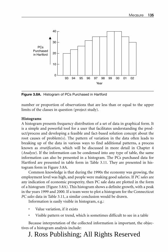
number or proportion of observations that are less than or equal to the upperlimits of the classes in question (project study).
Histograms A histogram presents frequency distribution of a set of data in graphical form. Itis a simple and powerful tool for a user that facilitates understanding the prod-uct/process and developing a feasible and fact-based solution concept about theroot causes of problem(s). The pattern of variation in the data often leads tobreaking up of the data in various ways to find additional patterns, a processknown as stratification, which will be discussed in more detail in Chapter 4(Analyze). If the information can be condensed into any type of table, the sameinformation can also be presented in a histogram. The PCs purchased data forHartford are presented in table form in Table 3.11. They are presented in his-togram form in Figure 3.8A.
Common knowledge is that during the 1990s the economy was growing, theemployment level was high, and people were making good salaries. If PC sales areany indication of economic prosperity, then PC sale data are plotted in the formof a histogram (Figure 3.8A). This histogram shows a definite growth, with a peakin the years 1999 and 2000. If a team were to plot a histogram for the ConnecticutPC sales data in Table 3.11, a similar conclusion would be drawn.
Information is easily visible in histogram, e.g.:
• Value variation, if it exists
• Visible pattern or trend, which is sometimes difficult to see in a table
Because interpretation of the collected information is important, the objec-tives of a histogram analysis include:
Measure 135
40
10
30
20
0
PCsPurchasedin Hartford
93 94 95 96 97 98 99 00 01 02
Year
Figure 3.8A. Histogram of PCs Purchased in Hartford
J. Ross Publishing; All Rights Reserved
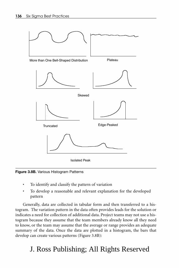
• To identify and classify the pattern of variation
• To develop a reasonable and relevant explanation for the developedpattern
Generally, data are collected in tabular form and then transferred to a his-togram. The variation pattern in the data often provides leads for the solution orindicates a need for collection of additional data. Project teams may not use a his-togram because they assume that the team members already know all they needto know, or the team may assume that the average or range provides an adequatesummary of the data. Once the data are plotted in a histogram, the bars thatdevelop can create various patterns (Figure 3.8B):
136 Six Sigma Best Practices
More than One Bell-Shaped Distribution Plateau
Skewed
Truncated Edge-Peaked
Isolated Peak
Figure 3.8B. Various Histogram Patterns
J. Ross Publishing; All Rights Reserved

Bell-shaped distribution. The most typical and natural type of data distribu-tion from a process is a bell-shaped distribution. A non bell-shaped distributionmay also be obtained.
More than one-bell-shaped distribution (multimodal frequency distribu-tion). This pattern can be the result of a combination of two or more bell-shapeddistributions, suggesting that the data are from two or more processes.
Plateau distribution. This pattern is most likely the result of several differentbell-shaped distributions evenly spread throughout the range of the data.
Skewed distribution. A skewed pattern may be skewed either to the left or tothe right. This pattern generally occurs when there is a practical limit or a speci-fication limit on one side which is relatively close to the nominal value. These dis-tributions are not considered to be undesirable, but the team should question theimpact of these values in the long “tail” data.
Truncated distribution. This type of distribution has generally smooth, bell-shaped distributions, with a part of the distribution removed through externaldecisions, e.g., a 100% inspection or a review process. These data removal effortsare additional costs and therefore should be good candidates for removal.
Edge-peaked distribution. This distribution occurs when the extended “tail”data of the distribution have been removed and lumped into a single category atthe edge of the range of the data. For example, the male population of the U.S. ispresented in a histogram, in which each bar represents a certain height group: <5feet, ≥5 feet, but <5 feet, 1 inch, ≥5 feet, 1 inch, but <5 feet, 2 inches, …, >5 feet,11 inches. The last bar represents everyone 5 feet, 11 inches and taller. Therefore,all males of height 6 feet, 6 feet, 1 inch, 6 feet, 2 inches, etc. are lumped into a sin-gle category at the edge of the range of the data. Most of the time, this shape indi-cates inaccurate recording of the data.
Isolated peak distribution. This pattern indicates a high probability that twoseparate processes are at work. The small size of the second peak indicates thepresence of unusual conditions.
Box Plot Box plots8 are similar to histograms. They provide a graphic summary of the vari-ation in a given set of data. The box plot is useful when working with small sets ofdata or when comparing several different sets of data.
A box plot displays: the three quartiles — first, d(Q1), median, d(M), andthird, d(Q3); the minimum (lowest value); and the maximum (highest value) ofthe data set on a rectangular box. The data are aligned either horizontally or ver-tically. Horizontally laid-out data goes from left to right, and vertically laid-outdata goes from bottom up. The logic for the five values is as follows:
• Arrange data in ascending order (from smallest to largest) and let thenumber of observations in the data set be n.
Measure 137
J. Ross Publishing; All Rights Reserved

• First quartile value, d(Q1) = Depth of the first quartile, where depth isthe number of observations (data points) to count from the begin-ning of the ordered data set.
d(Q1) = (n + 2)/4
If the value of d(Q1) includes a fraction/decimal, the quartile value isinterpolated.
• Median value, d(M) = Depth of median
d(M) = (n + 1)/2
Same rule applies as above.
• Third quartile value, d(Q3) = Depth of third quartile
d(Q3) = ((3)n + 2)/4
Same rule applies as above.
• Lowest and highest values are self-explanatory.
Example 3.5: Develop a Box Plot
Utilize the PC sales data from Hartford (see data in Table 3.11) and develop a boxplot. There are ten observations (n = 10). Arrange these observations in anascending order: 20, 25, 28, 30, 32, 35, 35, 35, 40, 40.
Lowest value = 20
Highest value = 40
d(Q1) = (10 + 2)/4 = 3
d(M) = (10 + 1)/2 = 5.5
d(Q3) = ((3)(10) + 2)/4 = 8
Therefore,
First quartile value, Q1 = 28
Median value = 33.5
Third quartile value, Q3 = 35
The generated box plot is presented in Figure 3.9. The box plot indicates thatthe distribution of PC sales is not fairly symmetric around the central valuebecause the lowest and the highest values and the length of the left and the rightboxes around the median are not the same.
A schematic box plot is similar to box plot; it is created in MINITAB. Aschematic box plot follows rules:
138 Six Sigma Best Practices
J. Ross Publishing; All Rights Reserved

• There are five values, similar to a box plot.
• The whiskers are now limited and are called the lower adjacent valueand the upper adjacent value instead of the lowest and the highest val-ues. (Note: Whiskers are the connecting lines between the lower adja-cent value and the Q1 box and between the upper adjacent value andthe Q3 box.)
• Observation values beyond the adjacent values are called outliers andare generally identified with an asterisk (*).
• A new value needs to be calculated, the inter quartile range (IQR).The IQR is the difference between Q3 and Q1.
• Determine the lower adjacent value, which is defined as the smallestobservation (collected data) = Q1 – (1.5) (IQR).
• Determine the upper adjacent value, which is defined as the largestobservation (collected data) = Q3 + (1.5) (IQR).
• Plotting follows the same rules as for the box plot.
3.4.2 Bar Graphs and Stacked Bar GraphsBar graphs and stacked bar graphs are an extension of histograms. These graphsare particularly effective in presenting data about qualitative or discrete quantita-tive variables. Bar graphs are often used to show a comparison between groups.Examples are presented in Figures 3.10A, 3.10B, and 3.10C. Stacked bar graphsplace the bars for each group on top of each other. A sample graph is presented inFigure 3.10D. These graphs present the data by a series of noncontiguous horizon-tal bars or vertical columns, the length of which are proportional to the values thatare to be depicted. A large amount of information can be summarized in a smallarea, communicating complex situations concisely and clearly.
Bar graphs are useful when comparing individual bars within a group as wellas the same subgroup across several groups. Stacked bar graphs are useful in
Measure 139
33.5
Thousands of PC Sold
20 28 35 40
15 25 35 45
Figure 3.9. Box Plot for Hartford PC Sales Data
J. Ross Publishing; All Rights Reserved

emphasizing the total of all the parts and the contribution of the individual piecesto the total. Stacking should be done only when the sum of the independent vari-ables is meaningful. For example, in the example of the Connecticut SwimmingClub, employee composition is divided into two groups—female and male. Astacked bar graph displays the results. Use a stacked bar graph if higher impor-
140 Six Sigma Best Practices
WhiteMale
WhiteFemale
BlackMale
BlackFemale
HispanicMale
HispanicFemale
0 1 2 3 4
Number of Employees
HispanicFemale
HispanicMale
BlackFemale
BlackMale
WhiteFemale
WhiteMale
4
3
2
1
Number ofEmployees
Figure 3.10A. Horizontal Bar Graph of Connecticut Swimming Club’s EmployeeComposition (Hypothetical Data)
Figure 3.10B. Vertical Bar Graph of Connecticut Swimming Club’s EmployeeComposition (Hypothetical Data)
J. Ross Publishing; All Rights Reserved

tance is given on the total of the components and the contribution of the eachcomponent to that total.
A grouped bar graph places more than one bar at each value for the inde-pendent variables, e.g., a bar graph that is developed to compare the number ofcustomers served by a service company for 3 years by major cities in theMidwestern part of the U.S. (Chicago, Kansas City, Detroit, and Milwaukee). Usea grouped bar graph if the individual variable data do not add up to a meaning-ful simple total or to facilitate the comparison of not only the individual barswithin a group, but also the bars of the same subgroup across several groups. Inthe above example, the graph not only compares the 3 years of service data withineach major city in the Midwestern states, but it also compares service data acrossthe cities.
Measure 141
4
3
2
1
HispanicFemale
HispanicMale
BlackFemale
BlackMale
WhiteFemale
WhiteMale
Number ofEmployees
4
3
2
1
Number ofEmployees
7
6
5
Female Male
White
Black
Hispanic
White
Black
Hispanic
Figure 3.10C. Grouped Bar Graph of Connecticut Swimming Club’s EmployeeComposition (Hypothetical Data)
Figure 3.10D. Stacked Bar Graph of Connecticut Swimming Club’s EmployeeComposition (Hypothetical Data)
J. Ross Publishing; All Rights Reserved

3.4.3 Pie ChartsTypically, a pie chart is a segmented circle that is able to portray divisions (pro-portionate distribution) of some aggregate provided the number of divisions isnot excessive. Pie charts are generally utilized to show relative contribution/com-position of a whole (also achieved with stacked bar graphs). A sample pie chart ispresented in Figure 3.11.
In Figure 3.11, resource employment by race (e.g., black, Hispanic, and white)at the Connecticut Swimming Club clearly stands out: white personnel substan-tially outnumber other races. To draw a pie chart:
• Determine the percentage for each category.
• Convert the percentage values into degrees of angles by taking the cal-culated percentage of 360 degrees.
• Draw a circle and mark the segments of the pie chart.
• Label the segments and entitle the chart.
Pie charts can also be used to compare two or more groups and their distri-bution within each group, e.g., comparing the employment distribution by raceamong two or more swimming clubs.
3.4.4 Line Graphs (Charts), Control Charts, and Run ChartsSeveral types of charts are utilized to describe information changes over time.Three types of charts (line, control, and run) will now be described.
142 Six Sigma Best Practices
Black Hispanic
White
Figure 3.11. Resources Distribution Pie Chart (Hypothetical Data)
J. Ross Publishing; All Rights Reserved

Line Graphs (Charts)Line charts are useful for presenting the evolution of given variables over time.The time increments can be large or small. A line chart can be utilized when bothvariables being compared are continuous (or almost continuous), e.g., tempera-ture, quantities, time, length, etc. Line charts are also useful for looking at trends.Line charts are drawn on a regular arithmetic scale as well as on a semilogarith-mic scale. An example is presented in Figure 3.12. The chart in Figure 3.12 showsthe trend in the number of houses sold in the state of Connecticut.
A line graph can be developed by following these instructions:
• Determine the range of the Y-axis (ordinate) and the size of eachincrement. Label the ordinate, including the unit of measure.
• Determine the range on the X-axis (abscissa) and the size of eachincrement. Label the abscissa, including the unit of measure.
• Draw X- and Y-axes (and a grid if needed).
• Plot data points.
• Connect the points with a line
• Label and entitle the graph.
Control Charts Business leaders know that there is an inherent variability in any data series,whether the series describes the size of inventories, customer service time, laborcosts, or even the loss of regular customers. Control charts are graphical devices
Measure 143
Thousands ofHomes Sold
40
30
20
10
093 94 95 96 97 98 99 00 01 02
Year
Figure 3.12. Line Chart—Home Sales in Connecticut (Hypothetical Data)
J. Ross Publishing; All Rights Reserved

that highlight the average performance of data series and the dispersion aroundthe average. Control charts are important tools in statistical process control. Theaverage performance of the past is viewed as the standard to which to current per-formance is compared. Typical dispersion of the past is used to set allowable lim-its for current performance. When plotting new data, immediately obvious iswhether the data fall within the range of the expected or whether there are unde-sirable trends that need immediate management attention.
Control charts are also utilized to detect assignable causes. The user (the per-son using the control chart) is responsible for identifying the underlying rootcause for an out-of-control condition, for developing and implementing anappropriate corrective action, and then following up to ensure that the assignablecause has been eliminated from the process. Remember these key points:
1. A state of statistical control is not a natural state for most processes.
2. The proper use of control charts will result in the elimination ofassignable causes, yielding the process in-control and reducedprocess variability.
3. A control chart is ineffective without a system to develop and imple-ment corrective actions that attack the root cause of problems.Business leadership and the participating group’s involvement areusually necessary to accomplish this.
The user acquires an ability to interpret control charts accurately throughexperience. Critical and necessary are that the user has a thorough familiarity withboth the statistical foundation of control charts and the nature of the processitself. Control charts are time-ordered graphical presentations of data that plotprocess variation over time. The centerline for the population represents theprocess average or middle point, while the centerline for the sample is the plottedmeasure. The sample centerline is expected to vary randomly in relation to thepopulation centerline. Upper and lower control limits define the area—threestandard deviations on either side of the centerline. These control limits reflectthe expected range of variation for that process. A sample chart is presented inFigure 3.13. Terminology and symbols used are defined as:
μ = Centerline for population (population mean)
⎯X= Centerline for sample (sample mean)
σ = Population’s standard deviation
s = Sample’s standard deviation
n = Number of times standard deviation from the mean
UCL (upper control limit) = μ + n σ for population
= ⎯X + n s for sample
144 Six Sigma Best Practices
J. Ross Publishing; All Rights Reserved

LCL (lower control limit) = μ – n σ for population
= ⎯X– n s for sample
It is important that the data originally measured can be converted into “stan-dard scores” defined by their own means and standard deviations (to be discussedin more detail in Section 6.4, Statistical Process Control (SPC) Techniques, ofChapter 6, Control.)
Run Charts Run charts are simple graphical devices with time-ordered plots that do not iden-tify any limits. These charts can be used to test the presence of special causes. Asample chart is presented in Figure 3.14.
3.4.5 Mean, Median, and ModeThe most important summary measures of central tendency are the mean, themedian, and the mode. Keeping their meanings distinct is important so that eachsummary measure of central tendency can be used appropriately.
Mean Among measures of central tendency, the most widely known measure is themean. The correct terminology is the arithmetic mean, but this measure is alsoreferred as the average. Adding all the data and dividing by the number of obser-vations calculates the average. The average is strongly affected by extreme values(see Example 3.6). The following are symbolic expressions of the mean:
Xi = Observed value
where:
Measure 145
UCL
Centerline (μ)
LCL
Time
Measure
Figure 3.13. Control Chart and Its Components
J. Ross Publishing; All Rights Reserved

i = 1, 2, 3, …, n (n = Number of values in a sample)
i = 1, 2, …, N (N = Number of values in a population)
μ = Population mean
⎯X = Sample mean
Median Another important measure of central tendency, but quite different in naturefrom the mean, is the median. If the values are arranged in an ordered array ofdata, then the number of observations above and below the median will be equal.The median value is not affected by the extreme values (see Example 3.6):
• If the number of observations is even, the median is the average of thetwo observations nearest the middle.
• If the number of observations is odd, the median is the middle dataobservation.
Mode The mode is defined as the most frequently occurring value in a data set (seeExample 3.6).
XX X X
n
X
nn
ii
n
...=
+ + += =
∑1 2 1
μ =+ + +
= =∑X X X
N
X
NN
ii
N
1 2 1...
146 Six Sigma Best Practices
Time
Measure
Figure 3.14. Run Chart and Its Components
J. Ross Publishing; All Rights Reserved

Example 3.6: A Survey of Process Engineer Experience
A survey of the experience of process engineers in a company was conducted, pro-viding the following data:
Process engineer 1 2 3 4 5 6 7 8
Experience (years) 2 2 4 5 6 6 6 9
Calculate the mean, median, and mode for the process engineers’ experience.
Solution:
Mode = 6 years
3.4.6 Range, Variance, and Standard DeviationKnowledge of the variability or the distribution of data around their center oflocation is critical in many situations. Consider a person making a decision aboutwhich one of two businesses he/she should enter. Both businesses may promisethe same median income, yet the incomes expected in one type of business maybe scattered widely about the mean, while the expected incomes in the other busi-ness fall within a relatively narrow range of the median. Depending on their atti-tudes about risk, different people will evaluate these two business prospectsdifferently.
Range The difference between the largest and the smallest observations in a set ofungrouped data is the range.
Variance The variance is a much more important measure of distribution, which is calcu-lated by averaging the squares of the individual deviations from the mean.
Standard DeviationThe standard deviation is the most important measure of dispersion. The squareroot of the variance is known as the standard deviation:
Median years.=+
=5 6
25 5
Mean X, =+ + + + + + +
=2 2 4 5 6 6 6 9
8
440
85= years
Measure 147
J. Ross Publishing; All Rights Reserved
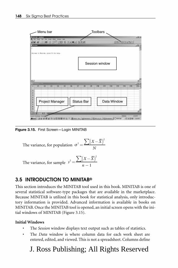
The variance, for population
The variance, for sample
3.5 INTRODUCTION TO MINITAB®
This section introduces the MINITAB tool used in this book. MINITAB is one ofseveral statistical software-type packages that are available in the marketplace.Because MINITAB is utilized in this book for statistical analysis, only introduc-tory information is provided. Advanced information is available in books onMINITAB. Once the MINITAB tool is opened, an initial screen opens with the ini-tial windows of MINITAB (Figure 3.15).
Initial Windows
• The Session window displays text output such as tables of statistics.
• The Data window is where column data for each work sheet areentered, edited, and viewed. This is not a spreadsheet. Columns define
sX X
n2
2
1=
−( )−
∑
σ 2
2
=−( )∑ X X
N
148 Six Sigma Best Practices
Menu bar Toolbars
Session window
Project Manager Status Bar Data Window
Figure 3.15. First Screen—Login MINITAB
J. Ross Publishing; All Rights Reserved

variables. Variable names can be listed above the first row. There canbe more than one data window.
• Graph windows are not displayed in Figure 3.15. These windows dis-play graphs also. Up to 100 graph windows can be open at a time.
Menus and Tools
• The Menu Bar is where commands are chosen.
• The Standard Toolbar displays buttons for commonly used functions.The buttons change depending on which MINITAB window is active.
• The Project Manager Toolbar provides shortcuts to Project Managerfolders.
• The Status Bar displays explanatory text whenever the cursor pointsto a menu item or Toolbar button.
• Shortcut Menus appear when right-clicking on any window inMINITAB or on any folder in Project Manager. The menu displays themost commonly used functions for that window or folder.
After clicking on Project Manager (PM) tool bar, the PM screen opens (seeFigure 3.16). The left-hand column of the screen is a folder that allows navigating,viewing, and manipulating various parts of the project. By right-clicking on eitherthe folders or the folder contents, a variety of menus can be accessed. Folder con-tents and their uses are listed in Table 3.12.
Measure 149
Folders
Figure 3.16. Project Manager Screen
J. Ross Publishing; All Rights Reserved
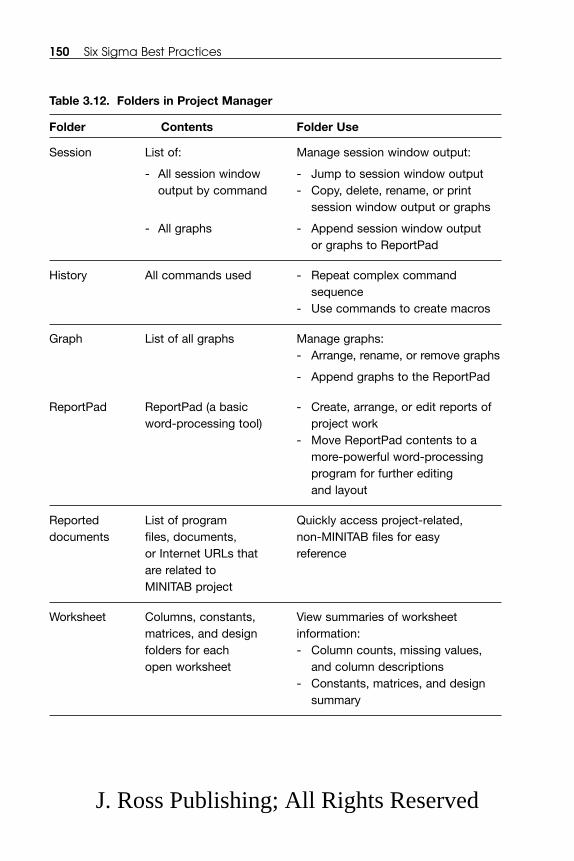
150 Six Sigma Best Practices
Table 3.12. Folders in Project Manager
Folder Contents Folder Use
Session List of: Manage session window output:
- All session window - Jump to session window outputoutput by command - Copy, delete, rename, or print
session window output or graphs
- All graphs - Append session window output or graphs to ReportPad
History All commands used - Repeat complex command sequence
- Use commands to create macros
Graph List of all graphs Manage graphs: - Arrange, rename, or remove graphs
- Append graphs to the ReportPad
ReportPad ReportPad (a basic - Create, arrange, or edit reports ofword-processing tool) project work
- Move ReportPad contents to amore-powerful word-processingprogram for further editing and layout
Reported List of program Quickly access project-related,documents files, documents, non-MINITAB files for easy
or Internet URLs that reference are related to MINITAB project
Worksheet Columns, constants, View summaries of worksheetmatrices, and design information:folders for each - Column counts, missing values,open worksheet and column descriptions
- Constants, matrices, and design summary
J. Ross Publishing; All Rights Reserved

Menu Bar—File CommandThe file menu is very similar to that of other Windows packages. Only active win-dows can be saved. Window information is presented in Figure 3.17.
Other Frequently Used Commands
• Edit
• Manip
• Calc
• Stat
• Graph
• Editor
• Window
• Help
Measure 151
Open/Save Project File
Open/Save Worksheet
Open/Save Graph
Export/Import Special Text File
Print Window
Exit
Figure 3.17. File Command from the Menu Bar
J. Ross Publishing; All Rights Reserved

Data WindowThe Data window is a most critical window. Three types of data entered in theData window:
• Numeric
• Date
• Text
Each column is identified as C1, C2, C3, and …. If the first row cell of any col-umn carries a date, the column number is extended with “-D.” If the first row cellof any column carries text, the column number is extended with “-T.” A sampledata window is presented in Figure 3.18.
Typing Data in the Data Window To enter a value in a Data window cell, click on the cell, type a value, and pressEnter. Multiple values can be entered in any order: row by row, column by col-umn, or in blocks. Cells contain values only, not formulas as in Excel. To performmathematical functions, use:
Calc > Calculator
152 Six Sigma Best Practices
Column number
Column name
Data direction arrow
• Data window body consists of rows and columns• Each column generally represents a variable• Each row generally represents an individual case or observation• Only one data window can be open at a time
Scroll Bars
Figure 3.18. Data Window in MINITAB
J. Ross Publishing; All Rights Reserved

Data can also be entered by:
• Copy/Paste from MINITAB and other sources such as Windows soft-ware (e.g., Excel)
• Generated from a set patterned data, random data, and storage
• Imported from many commonly used software packages (e.g., Excel,ASCII files)
If a column defined as “text” needs to be converted to “numeric,” simply fol-low the command:
Manip > Change Data Type > Text to numeric
Dialog boxes will appear. Fill in the dialog boxes to indicate the column to bechanged and where it is to be stored.
To move between all three data types (Text, Date, and Numeric), follow thecommand:
Manip > Change Data Type
Entering Data in Columns, Rows, or Blocks
To enter data from one column to the next column:
• Click the data direction arrow so it points down.
• Enter data, pressing Tab or Enter to move the active cell. PressCtrl+Enter to move the active cell to the top of the next column.
To enter data from one row to the next row:
• Click the data direction arrow so it points to the right.
• Enter data in the cells of a row. Press Ctrl+Enter to move the activecell to the beginning of the next row.
To enter data within a block:
• Highlight the selected blocked area.
• Enter data. The active cell moves only within the selected area.
• To unselect the area, press an arrow key or click anywhere in the Datawindow.
Inserting Empty Cells, Rows, and Columns
• Select one or more cells.
• Choose Editor > Insert Cells/Insert Rows/Insert Columns.
Measure 153
J. Ross Publishing; All Rights Reserved
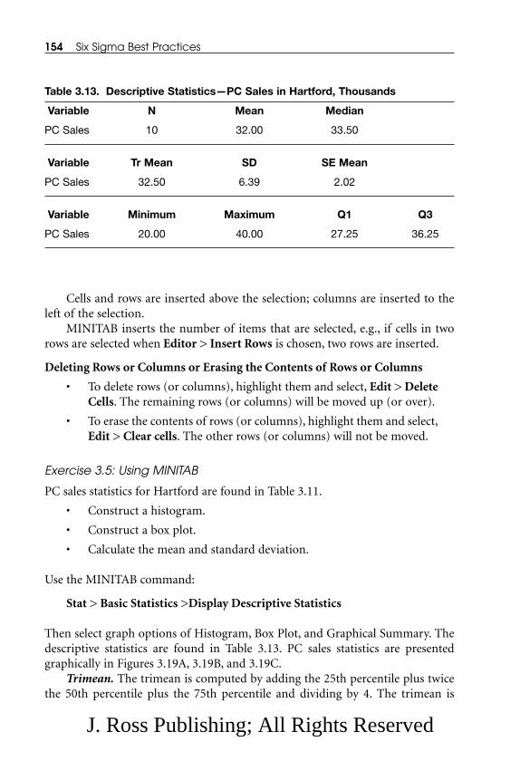
Cells and rows are inserted above the selection; columns are inserted to theleft of the selection.
MINITAB inserts the number of items that are selected, e.g., if cells in tworows are selected when Editor > Insert Rows is chosen, two rows are inserted.
Deleting Rows or Columns or Erasing the Contents of Rows or Columns
• To delete rows (or columns), highlight them and select, Edit > DeleteCells. The remaining rows (or columns) will be moved up (or over).
• To erase the contents of rows (or columns), highlight them and select,Edit > Clear cells. The other rows (or columns) will not be moved.
Exercise 3.5: Using MINITAB
PC sales statistics for Hartford are found in Table 3.11.
• Construct a histogram.
• Construct a box plot.
• Calculate the mean and standard deviation.
Use the MINITAB command:
Stat > Basic Statistics >Display Descriptive Statistics
Then select graph options of Histogram, Box Plot, and Graphical Summary. Thedescriptive statistics are found in Table 3.13. PC sales statistics are presentedgraphically in Figures 3.19A, 3.19B, and 3.19C.
Trimean. The trimean is computed by adding the 25th percentile plus twicethe 50th percentile plus the 75th percentile and dividing by 4. The trimean is
154 Six Sigma Best Practices
Table 3.13. Descriptive Statistics—PC Sales in Hartford, Thousands
Variable N Mean Median
PC Sales 10 32.00 33.50
Variable Tr Mean SD SE Mean
PC Sales 32.50 6.39 2.02
Variable Minimum Maximum Q1 Q3
PC Sales 20.00 40.00 27.25 36.25
J. Ross Publishing; All Rights Reserved
almost as resistant to extreme scores as the median. It is also less subject to sam-pling fluctuations than the arithmetic mean in extremely skewed distributions.The trimean is less efficient than the mean for normal distributions. The trimeanis a good measure of central tendency and is probably not used as much as itshould be.
Standard error of the mean (SE mean). The standard deviation of the distri-bution of sample means is commonly called the standard error of the mean.Standard deviation of the distribution of sample means = (1/√n) standard devia-tion of the universe of individual values.
3.6 DETERMINING SAMPLE SIZE
Before beginning to collect data, a team must know the sample size. This sectionwill discuss determining the sample size.
To prove that a process has been improved, the team must measure theprocess capability before and after improvements have been implemented. Thismeasurement allows the team to quantify the process improvement (e.g., defectreduction or productivity improvement) and translate the effects into estimatedfinancial results. Improved financial results are something that business leadersunderstand and appreciate. If data are not readily available for the process, theteam must answer:
• How many members of the population should be selected to ensurethat the population is properly represented?
• If the data have been collected, how would the team determine if it hasenough data?
Determining sample size is an important issue because samples that are toolarge can waste time, resources, and money, while samples that are too small canlead to inaccurate results. In many situations, the minimum sample size is neededto estimate a process parameter, such as the population mean μ.
Let,–X = Sample mean based on the collected data. This sample mean is gen-
erally different from the population mean μ. The difference between the sampleand population means can be considered to be an error. If E = margin of error,i.e., the maximum difference between the observed sample mean
–X and the true
value of the population mean μ, then:
E = Zα/2 (σ/√n)
where:
Measure 155
J. Ross Publishing; All Rights Reserved

20 30 40
PC Sales in Hartford, Thousands
Figure 3.19A. Box Plot—PC Sales Statistics
4035302520
95% Confidence Interval for Mu
363126
95% Confidence Interval for Median
Variable: PC Sale in H
26.9730
4.3983
27.4257
Maximum3rd QuartileMedian1st QuartileMinimum
NKurtosisSkewnessVarianceStDevMean
P-Value:A-Squared:
36.7117
11.6738
36.5743
40.000036.250033.500027.250020.0000
10-1.8E-01-5.5E-0140.8889 6.394432.0000
0.6150.264
95% Confidence Interval for Median
95% Confidence Interval for Sigma
95% Confidence Interval for Mu
Anderson-Darling Normality Test
Descriptive Statistics
Figure 3.19B. Descriptive Statistics—PC Sales
156 Six Sigma Best Practices
J. Ross Publishing; All Rights Reserved

Zα/2 = Critical value, the positive Z value that is at the vertical boundary forthe area of α/2 in the right tail of the standard normal distribution(Figure 3.20)
σ = Population standard deviation
n = Sample size
Reorganize the above formula, and solve for the sample size necessary to pro-duce results accurate to a specified confidence and margin of error:
n = [(Zα/2 σ)/E]2
This formula can be used when the user knows the process σ and wants todetermine the sample size necessary to establish, with a confidence of 1 – α, themean value μ to within ± E. The user can still use this formula if the population’sstandard deviation σ is not known and the sample size is small (even though it isunlikely that the user knows σ when the population mean is not known). The usermay be able to determine σ from a similar process or from a pilot test/simulation.Consider Example 3.7.
Example 3.7: Sample Size Determination
A Quality Group in The Connecticut Precision Manufacturing Company needs toestimate the manufactured blade length. How many blades must be randomly
Measure 157
1993 1994 1995 1996 1997 1998 1999 2000 2001 2002
40
30
20
Year
Sum
of H
artfo
rd P
Cs
Pur
chas
ed
Figure 3.19C. Histogram—PC Sales
J. Ross Publishing; All Rights Reserved

selected for measuring the blade length to be 99% sure that the sample mean iswithin 0.0005 mm from the population mean μ = 5.00 mm? Assume that a previ-ous measurement test has shown that σ = 0.002 mm.
Solving for the sample size, n:
A 99% degree of confidence corresponds to α = 0.01.
Each of the tails in the normal distribution has an area of α/2 = 0.005.
Therefore, at Zα/2 = 0.005 = 2.575
Now, n = [(Zα/2 s)/E]2
= [(2.575 � 0.002)/(0.0005)]2
= 106.09
Therefore, the sample size should be at least (rounded up) 107 blades ran-domly selected. With this sample, the Quality Group will be 99% confident thatthe sample mean will be within 0.0005 mm of the true population mean (bladelength μ = 5 mm).
Exercise 3.6: Estimating Internet Use
To start an Internet service provider (ISP) business, estimating the averageInternet usage by households in 1 week is required for a business plan and model.How many households must be randomly selected to be 95% sure that the sam-ple mean is within 2 minutes of the population mean μ = 200 minutes? Assumethat a previous survey of household usage revealed σ = 10.75 minutes.
3.7 PROBABILISTIC DATA DISTRIBUTION
A great appreciation for probability theory comes from observing the outcome ofa real experiment. These experiments are called random experiments. Commoncharacteristics of a random experiment include:
158 Six Sigma Best Practices
Z = 0
α/2 α/2
Zα/2
Figure 3.20. Critical Value Location
J. Ross Publishing; All Rights Reserved

• The outcome of the experiment cannot be predicted with certainty.
• Under unchanged conditions, the experiment could be repeated withthe outcomes appearing in a haphazard manner. As the experiment-repeating process increases, a certain pattern in the frequency of out-come emerges.
To illustrate random experiments with an associated sample space, considerthe following example:
Toss a pair of dice and observe the “up” faces. The total sample space is shownin Table 3.14. Suppose a random variable X is defined as the sum of the “up” facesas events in X that are defined as RX. Then RX = (2, 3, 4, 5, 6, 7, 8, 9, 10, 11, 12) andthe probabilities are (1/36, 2/36, 3/36, 4/36, 5/36, 6/36, 5/36, 4/36, 3/36, 2/36,1/36), respectively. Assuming the dice are true and are equally likely, there will be36 outcomes as listed above. The same output is presented in the equivalent eventsin Table 3.15.
Product/process data may be deterministic or probabilistic. If the data areprobabilistic, data may follow the shape of one or more probabilistic distribu-tions. The remainder of this section will discuss commonly found probability dis-tributions as the product/process data are analyzed: normal, Poisson, exponential,binomial, gamma, and Weibull.
3.7.1 Normal DistributionThe most important of all distribution formulas for continuous variables is thatfor the normal distribution. The distribution is defined by two parameters: mean(μ) and standard deviation (σ)/variance (σ2). A random variable X is said to havea normal distribution, with mean μ(– ∞ < μ < ∞) and variance (square of stan-dard deviation) σ2 > 0. The density function in general form is:
where – ∞ < μ < ∞f X eX
( )=⎛
⎝⎜⎜⎜
⎞
⎠⎟⎟⎟⎟
−−⎛
⎝⎜⎜⎜⎜
⎞
⎠⎟⎟⎟⎟1
2
1
2
σ
μσ
Π
22
Measure 159
Table 3.14. Possible Outcomes When Tossing a Pair of Fair Dice
(1,1), (1,2), (1,3), (1,4), (1,5), (1,6),
(2,1), (2,2), (2,3), (2,4), (2,5), (2,6),
(3,1), (3,2), (3,3), (3,4), (3,5), (3,6),
(4,1), (4,2), (4,3), (4,4), (4,5), (4,6),
(5,1), (5,2), (5,3), (5,4), (5,5), (5,6),
(6,1), (6,2), (6,3), (6,4), (6,5), (6,6)
J. Ross Publishing; All Rights Reserved
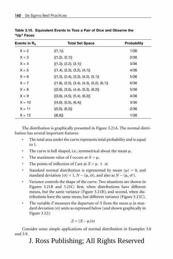
The distribution is graphically presented in Figure 3.21A. The normal distri-bution has several important features:
• The total area under the curve represents total probability and is equalto 1.
• The curve is bell shaped, i.e., symmetrical about the mean μ.
• The maximum value of f occurs at X = μ.
• The points of inflection of f are at X = μ ± σ.
• Standard normal distribution is represented by mean (μ) = 0, andstandard deviation (σ) = 1, N ~ (μ, σ), and also as N ~ (μ, σ2).
• Variance controls the shape of the curve. Two situations are shown inFigures 3.21B and 3.21C: first, when distributions have differentmeans, but the same variance (Figure 3.21B); and second, when dis-tributions have the same mean, but different variance (Figure 3.21C).
• The variable Z measures the departure of X from the mean μ in stan-dard deviation (σ) units as expressed below (and shown graphically inFigure 3.22):
Z = (X – μ)/σ
Consider some simple applications of normal distribution in Examples 3.8and 3.9.
160 Six Sigma Best Practices
Table 3.15. Equivalent Events to Toss a Pair of Dice and Observe the “Up” Faces
Events in RX Total Set Space Probability
X = 2 {(1,1)} 1/36
X = 3 {(1,2), (2,1)} 2/36
X = 4 {(1,3), (2,2), (3,1)} 3/36
X = 5 {(1,4), (2,3), (3,2), (4,1)} 4/36
X = 6 {(1,5), (2,4), (3,3), (4,2), (5,1)} 5/36
X = 7 {(1,6), (2,5), (3,4), (4,3), (5,2), (6,1)} 6/36
X = 8 {(2,6), (3,5), (4,4), (5,3), (6,2)} 5/36
X = 9 {(3,6), (4,5), (5,4), (6,3)} 4/36
X = 10 {(4,6), (5,5), (6,4)} 3/36
X = 11 {(5,6), (6,5)} 2/36
X = 12 {(6,6)} 1/36
J. Ross Publishing; All Rights Reserved

Measure 161
μ
F(X)
X
Figure 3.21A. Normal Distribution
Figure 3.21B. Normal Distribution with Different Means
Figure 3.21C. Normal Distribution with Different Variances
J. Ross Publishing; All Rights Reserved

Example 3.8: Repair of Turning Machine
Suppose that a turning machine has broken down and a repairperson is availableto repair the machine for 58 minutes. Assume that the repair process is normallydistributed with a mean repair time of 50 minutes and a standard deviation of 8minutes. What is the probability that the repairperson will repair the machine in58 minutes?
Solution:Repair time is normally distributed with:
Mean (μ) = 50 minutes
Standard deviation (σ) = 8 minutes
Repair time “X” = 58 minutes
162 Six Sigma Best Practices
Mean
SD
Standard Normal Distribution
Z = (X1 – Mean)/ SD
X1
1
Z
? Z
Mean = 0
Figure 3.22. Calculation of Z Value
J. Ross Publishing; All Rights Reserved

Now, calculate the value of Z, where Z = (X – μ)/σ:
Z = (58 – 50)/8 = 1
Probability (Z ≤ 1) = 0.8413
Therefore, there are 84.13% chances that the machine will be repaired in 58 min-utes.
Example 3.9: Weight of Components
The quantity of 300 small components is packed in a box. The weight of thesecomponents is an independent random variable with a mean weight of 5 gramsand a standard deviation of 1 gram. Twenty-five boxes of these small componentsare loaded on the platform of a material-handling device. Suppose the probabil-ity that the components on the platform will exceed 37.7 kilograms in weight isneeded (neglect both boxes and crate weight).
Solution:Let,
Y = X1 + X2 + … + X7500 represent the total weight of the components and
μY = 7500 (5) = 37,500 grams
= 37.5 kilograms
σY = σ √n
= (1) √7500
σY = 86.603
Then,
1 – Φ(2.309) = 1 – 0.98953= 0.01047
Therefore, the probability to exceed the weight of the small components (37.7kilograms) = 0.01047.
Distribution of Means of Samples from Any Universe All distributions of sample means (μX-bar) have certain properties in commonwith those of the parent population. Assuming random sampling, these proper-ties include:
P Y P Z>( )= >−⎛
⎝⎜⎜⎜
⎞
⎠⎟⎟37 700
37 700 37 500
86 603,
, ,
. ⎟⎟⎟
Measure 163
J. Ross Publishing; All Rights Reserved
• When selection of sample elements are statistically independentevents, typically referred to as “the large-population case,” where n < 0.05 N.
• The mean of the distribution of sample means (μX-bar) is the mean ofthe universe of individual values (μ) from which the samples aretaken, μX-bar = μ.
• The variance of the distribution of sample means (σ2X-bar) equals the
variance of the universe of individual values (σ2) divided by n, the sizeof the sample, σ2
X-bar = σ2/n. (This can also be written as: the standarddeviation of the distribution of sample means equals 1/√n times thestandard deviation of the universe of individual values, σX-bar = σ/n0.5.)
• The form of the distribution of sample means approaches the form ofa normal probability distribution as the size of the sample isincreased.
and where:
μX-bar = Sample mean
σ2X-bar = Sample variance
σX-bar = Sample standard deviation
–X = Sample mean
while:
μ, σ2, and σ = population mean, variance, and standard deviation, respec-tively
n = Sample size
N = Population
Example 3.10 has been developed to validate this relationship.
Example 3.10: Estimating Parameters
Suppose that census-type information is not available and cannot be easilyobtained. (In reality, thousands of engineers may be graduating with an engineer-ing degree from universities and colleges and starting their professional career.Collecting information about their starting annual salary would be very expensiveand time-consuming.) Therefore, a decision is made to estimate the three popu-lation parameters (mean, variance, and standard deviation) by taking a random
164 Six Sigma Best Practices
J. Ross Publishing; All Rights Reserved

sample of five engineers with their starting salaries in year 2004. The data are asfollows:
Engineer Annual Starting Salary ($K)
A 39B 41C 25D 55E 40
Because this is a small population, N = 5 and the summary statistics are
μ = ΣX/N = 200/5 = 40
= 452/5 = 90.4
σ = 9.508
Now take a sample of 3 (n = 3) without replacement from the above popula-tion (N = 5) and calculate the sample statistics (X, s2, and s) as presented in Table3.16. The possible number of samples of n = 3 out of the population of N = 5equals C5
3 = 10 samples.Now, if the statistics of data
–X (see Table 3.16) is calculated, then:
μX-bar = Σ–X/10 = 400/10 = 40
σ2X-bar = 15.1
σX-bar = 3.886
Now apply the logic presented above for a small population, where N = 5, andn = 3, then:
μX-bar = μ = 40 and
= 15.07
This validates the above concept.
σ X bar-2 90 4
3
5 3
5 1=
⎛
⎝⎜⎜⎜
⎞
⎠⎟⎟⎟⎟
−−
⎛
⎝⎜⎜⎜
⎞
⎠⎟⎟⎟⎟
.
σσ
X bar n
N n
N-2
2
1=
⎛
⎝⎜⎜⎜⎜
⎞
⎠⎟⎟⎟⎟
−−
⎛
⎝⎜⎜⎜
⎞
⎠⎟⎟⎟⎟
σμ2
2
=−( )∑ X
N
Measure 165
J. Ross Publishing; All Rights Reserved

The Central Limit Theorem Next is a discussion of the Central Limit Theorem with a large population. If thesum of n independent random variables is represented by a random variable Ythat satisfies certain general conditions, then for a very large n, Y is approximatelynormally distributed.
If n independent variables are X1, X2, …, Xn and these variables are identicallydistributed random variables with:
Mean E(Xi) = μ
Variance V(Xi) = σ2
Y = X1 + X2 + … + Xn
then:
has an approximate N(0,1) distribution.
An immediate question that comes to mind is “How large must n be to getreasonable results using the normal distribution to approximate the distributionof Y?” This is not an easy question to answer due to:
• The characteristics of the distribution of the Xi terms
• The meaning of the term “reasonable results”
However, Hines and Montgomery8 have an answer. From a practical stand-point, some crude rules of thumb can be given where the distribution of the Xi
terms falls into one of three arbitrarily selected groups:
1. Well-behaved—The distribution of Xi does not radically departfrom the normal distribution. There is a bell-shaped density that isnearly symmetric. In this case, practitioners in quality control andother areas of application find that n should be at least 4 (n ≥ 4).
2. Fairly well-behaved—The distribution of Xi has no prominentmode. It appears much like a uniform density. In this case, n ≥ 12is a commonly used rule.
3. Ill-behaved—The distribution has most of its measure in the “tails.”In this case, determining a rule is most difficult; however, in manypractical applications, n ≥ 100 should be satisfactory.
ZY n
nn =
− μ
σ
166 Six Sigma Best Practices
J. Ross Publishing; All Rights Reserved

Example 3.11: The Central Limit Theorem with a Large Population
Test the theory: “If the sum of n independent random variables is represented bya random variable Y that satisfies certain general conditions, then for a very largen, Y is approximately normally distributed” (a large population).
Utilizing the MINITAB software tool:
• Start the MINITAB software tool.
• Create some simulated data to test this theory.
• Use the following MINITAB commands to create 10 columns of datautilizing a normal distribution with a mean = 35 and a standard devi-ation = 4:
MINITAB > Calc > Random Data > NormalGenerate 300 RowsStore in C1 – C10Mean = 35Standard Deviation = 4
MINITAB > Calc > Row Statistics >Mean C1 – C10Store results into C11
MINITAB > Stat > Basic Stats > Display Descriptive Stat > C1 – C11
Measure 167
Table 3.16. Possible Sample of n = 3 Taken without Replacement from thePopulation of N = 5 and Its Statistics
Sample EngineersNumber in Sample
–X s2 s
1 ABC 35.00 76.00 8.718
2 ABD 45.00 76.00 8.718
3 ABE 40.00 1.00 1.00
4 ACD 39.67 225.33 15.01
5 ACE 34.67 70.33 8.386
6 ADE 44.67 80.33 8.963
7 BCD 40.33 25.33 15.01
8 BCE 35.33 80.33 8.963
9 BDE 45.33 0.33 8.386
10 CDE 40.00 225.00 15.00
Summary Statistics for Salary
J. Ross Publishing; All Rights Reserved

The expected standard deviation of mean = σ/√n:
Let, n = 9
Then, standard deviation of mean = 4/√9
= 1.333
What is the value of the standard deviation of mean in row C11?The process was repeated 10 times, with the results presented in row C11: the
sample mean is very close to the population mean (μ = 35, μX-bar = 34.99) and therelationship about the standard deviation is as follows:
σ = 3.99
σX-bar = 1.243 (which is close to 1.333)
This validates the concept of large population. The summary output fromMINITAB is shown in Table 3.17 and in Figures 3.23A and 3.23B. The plottedgraphs are C1: the distribution of individual observations (Figure 3.23A); and C11:the distribution of sample mean (Figure 3.23B). The MINITAB instructions are:
• MINITAB > Graph > Character Graph > Dotplot
• Variables: Select C1, Select C11, Check box Same scale for all vari-ables, OK
3.7.2 Poisson DistributionThe Poisson distribution is utilized when the user is interested in the occurrenceof a number of events of the same type. Therefore, the Poisson probability distri-bution associates probabilities with number of occurrences of some event withinspecified intervals of time or space as shown in Figure 3.24A by an asterisk (*).This exponential distribution instead associates probabilities with the variousgaps, shown by the values of X1 to X7 between the Poisson events.
The occurrence of each event is represented as a point on the time scale. Thedensity function is represented by f(n):
, n = 0, 1, 2, …
= 0 otherwise
where:
t = Time
λ = Constant factor
n = Number of occurrences
f nt e
n
n t
( ) =( ) −
!
λ λ
168 Six Sigma Best Practices
J. Ross Publishing; All Rights Reserved

The parameter, mean, and variance of the Poisson distribution are the expres-sions:
Parameter = λ
Mean (μ) = λt
Variance (σ2) = λt
A probability density function graph is presented in Figure 3.24B. Theparameter λ represents the expected occurrence of the event’s rate, e.g., customerarrival rate at a bank, plane landing rate at an airport’s runway, engine failure rateat a water pumping station, etc. Example 3.12 will make the concept even clearer.
Measure 169
C1 20.0 25.0 30.0 35.0 40.0 45.0
Dotplot: C1
Figure 3.23A. Distribution of Individual Observations (with Each Dot RepresentingUp to Four Points)
Dotplot: C11 : : .::
:::::::.:::::::
..:::::::: ..:::::::::::...
+---------+---------+---------+---------+---------+C11 20.0 25.0 30.0 35.0 40.0 45.0
Figure 3.23B. Distribution of Sample Mean
J. Ross Publishing; All Rights Reserved

Example 3.12: Plane Arrival Rates
Suppose planes have been arriving at an airport at the rate of two per minute dur-ing a Friday evening. The airport manager wants to know the probabilities of 6, 9,and 20 planes arriving between 8:00 and 8:10 p.m.
Assuming that plane arrivals are following the Poisson distribution in the example:
λ = 2 planes per minute
t = 10 minutes (time between 8:00 and 8:10 p.m.)
n = 6, 9, and 20 (number of plane arrivals during the specified time of10 minutes)
Since,
, n = 0, 1, 2, …
therefore, λt = 2 � 10 = 20:
(probability of 6 planes landing in defined period)f ne
( )( )
!.= = =
−
620
60 002
6 20
f nt e
n
n t
( ) =( ) −
!
λ λ
170 Six Sigma Best Practices
Table 3.17. Descriptive Statistics Output from MINITAB
Variable N Mean Median Tr Mean SD SE Mean
C1 300 34.595 34.794 34.585 3.991 0.230
C2 300 35.095 35.182 35.087 3.987 0.230
C3 300 34.896 34.786 34.907 3.804 0.220
C4 300 34.923 34.824 34.914 4.171 0.241
C5 300 34.870 34.682 34.865 3.915 0.226
C6 300 35.147 35.113 35.108 3.856 0.223
C7 300 34.909 35.013 34.951 3.875 0.224
C8 300 35.664 35.885 35.598 4.152 0.240
C9 300 34.798 34.861 34.714 3.995 0.231
C10 300 35.000 35.050 35.036 4.066 0.235
C11 300 34.990 35.041 34.998 1.243 0.072
J. Ross Publishing; All Rights Reserved
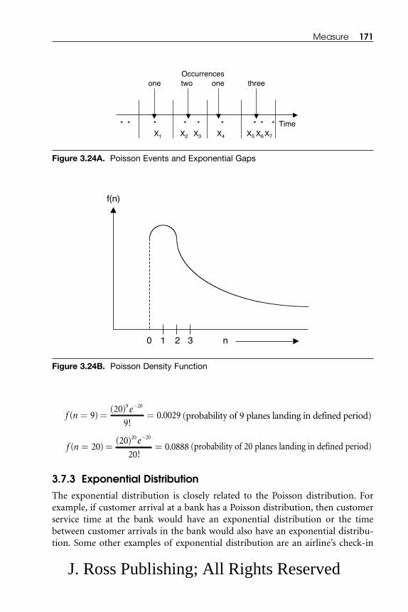
(probability of 9 planes landing in defined period)
(probability of 20 planes landing in defined period)
3.7.3 Exponential DistributionThe exponential distribution is closely related to the Poisson distribution. Forexample, if customer arrival at a bank has a Poisson distribution, then customerservice time at the bank would have an exponential distribution or the timebetween customer arrivals in the bank would also have an exponential distribu-tion. Some other examples of exponential distribution are an airline’s check-in
f ne
( )( )
!.= = =
−
2020
200 0888
20 20
f ne
( )( )
!.= = =
−
920
90 0029
9 20
Measure 171
* * * * * * * * *
one two one three
Time
Occurrences
X1 X2 X3 X4 X5 X6X7
Figure 3.24A. Poisson Events and Exponential Gaps
0 1 2 3 n
f(n)
Figure 3.24B. Poisson Density Function
J. Ross Publishing; All Rights Reserved

counter, filling a gas tank in an automobile at the gas station, getting checked outa supermarket’s checkout counter, etc. These examples are often assumed to havean exponential distribution.
The exponential distribution has density function:
f(X) = λe-λX X ≥ 0
= 0 otherwise
where the parameter λ is real and positive constant. The expected value (mean) is1/λ and the variance is 1/λ2. A probability density function graph is presented inFigure 3.25A.
Suppose a small bank has only one person to serve arriving customers and onaverage it takes 2 minutes to serve a customer. Therefore, the customer arrival rateper minute λ has to be less than 1/2; otherwise a customer would have to wait ina queue at the bank before being served.
The cumulative density function (CDF) of an exponentially distributed ran-dom variable FX(a) is given by:
for a ≥ 0
= 0 for a < 0
The function is presented in Figure 3.25B
For example, suppose that the life of a light bulb is assumed to have an expo-nential distribution. If the bulb lasted 500 hours, the probability of it lasting anadditional 40 hours is the same as the probability of it lasting an additional 40hours if the bulb has lasted 1000 hours. Therefore, the concept is that a brand newbulb is no “better” than one that has lasted 500 hours. The concept of exponentialdistribution is very important and one that is quite often overlooked in practicallife.
Now consider R(X), which is the probability of occurrence (failure) or relia-bility on [0, X]. Because X represents time, this is expressed as R(t) = e–λt, where tis the mission time. This concept is explained in Example 3.13.
Example 3.13: Engine Life
Three engines are subjected to a nonreplacement life test, which is to be termi-nated at 10 hours. Assume failure times to be exponentially distributed with amean life of 200 hours. As a test engineer for this test, estimate the probability
F a e dX eXX
a
a( ) = = −− −∫ λ λ λ
0
1
F a f X dXX
a
( ) =−∞∫ ( )
172 Six Sigma Best Practices
J. Ross Publishing; All Rights Reserved

that no failure will occur and the probability that one failure will occur. Utilize theconcept of exponential distribution.
Since mean time to failure = 200 hours, therefore, λ = 1/200 = a 0.005 engine fail-ure rate per hour.
The mission time is 10 hours, and the mission time reliability of the engine:
R(t = 10) = e–λt
R(t = 10) = e-0.005 (10) = 0.95123
Assume these three engines (i.e., A, B, and C) are identical.
Their probability of success:
P(A) = P(B) = P(C) = 0.95123
Their probability of failure (complementary probability):
P(–A) = P(
–B) = P(
–C) = 1 – 0.95123 = 0.04877
Measure 173
λ
0 X
f(X)
Figure 3.25A. Exponential Density Function
a0 +∞
Fx(a)
1
Figure 3.25B. CDF of the Exponential Distribution
J. Ross Publishing; All Rights Reserved
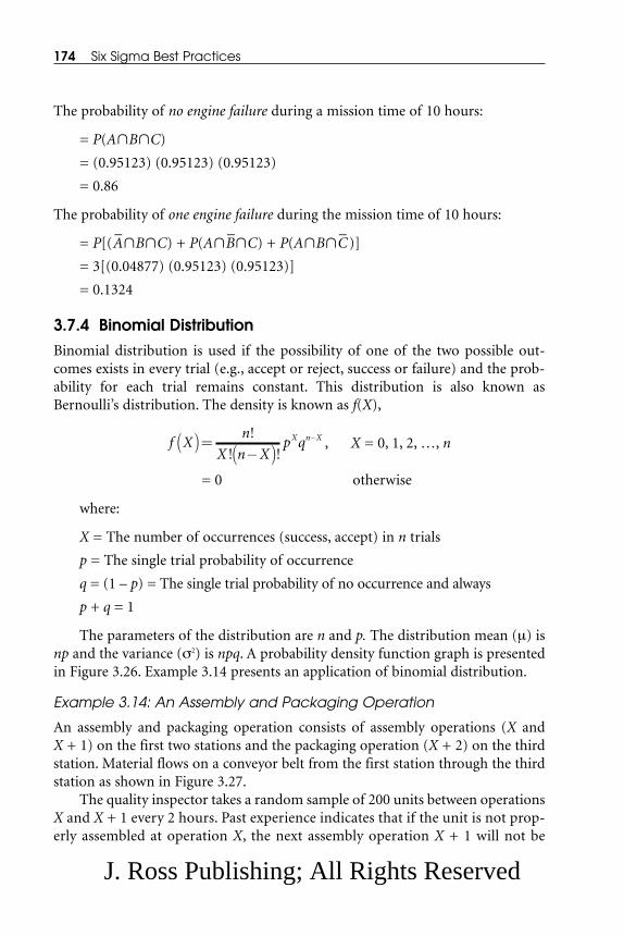
The probability of no engine failure during a mission time of 10 hours:
= P(A�B�C)
= (0.95123) (0.95123) (0.95123)
= 0.86
The probability of one engine failure during the mission time of 10 hours:
= P[(–A�B�C) + P(A�
–B�C) + P(A�B�
–C)]
= 3[(0.04877) (0.95123) (0.95123)]
= 0.1324
3.7.4 Binomial DistributionBinomial distribution is used if the possibility of one of the two possible out-comes exists in every trial (e.g., accept or reject, success or failure) and the prob-ability for each trial remains constant. This distribution is also known asBernoulli’s distribution. The density is known as f(X),
, X = 0, 1, 2, …, n
= 0 otherwise
where:
X = The number of occurrences (success, accept) in n trials
p = The single trial probability of occurrence
q = (1 – p) = The single trial probability of no occurrence and always
p + q = 1
The parameters of the distribution are n and p. The distribution mean (μ) isnp and the variance (σ2) is npq. A probability density function graph is presentedin Figure 3.26. Example 3.14 presents an application of binomial distribution.
Example 3.14: An Assembly and Packaging Operation
An assembly and packaging operation consists of assembly operations (X and X + 1) on the first two stations and the packaging operation (X + 2) on the thirdstation. Material flows on a conveyor belt from the first station through the thirdstation as shown in Figure 3.27.
The quality inspector takes a random sample of 200 units between operationsX and X + 1 every 2 hours. Past experience indicates that if the unit is not prop-erly assembled at operation X, the next assembly operation X + 1 will not be
f Xn
X n Xp qX n X( )=
−( )−!
! !
174 Six Sigma Best Practices
J. Ross Publishing; All Rights Reserved
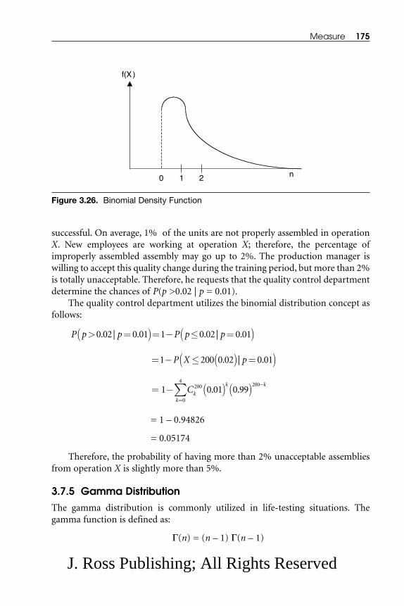
successful. On average, 1% of the units are not properly assembled in operationX. New employees are working at operation X; therefore, the percentage ofimproperly assembled assembly may go up to 2%. The production manager iswilling to accept this quality change during the training period, but more than 2%is totally unacceptable. Therefore, he requests that the quality control departmentdetermine the chances of P(p >0.02 | p = 0.01).
The quality control department utilizes the binomial distribution concept asfollows:
= 1 – 0.94826
= 0.05174
Therefore, the probability of having more than 2% unacceptable assembliesfrom operation X is slightly more than 5%.
3.7.5 Gamma DistributionThe gamma distribution is commonly utilized in life-testing situations. Thegamma function is defined as:
Γ(n) = (n – 1) Γ(n – 1)
= − ( ) ( )=
−∑ . .1 0 01 0 99200
0
4200
Ckk
k k
= − ≤ ( ) =( )1 200 0 02 0 01P X p. | .
P p p P p p> =( )= − ≤ =( )0 02 0 01 1 0 02 0 01. | . . | .
Measure 175
f(X )
0 1 2 n
Figure 3.26. Binomial Density Function
J. Ross Publishing; All Rights Reserved

If n is a positive integer, then:
Γ(n) = (n – 1)!
The gamma probability density function is presented as follows:
where X > 0
= 0 otherwise
where:
r = Shape parameter and
λ = Scale parameter
and these parameters are greater than zero, i.e., r > 0 and λ > 0.
r/λ = The distribution mean and
(r/λ)2 = The distribution variance
The gamma distribution is an extension of the exponential distribution.When r = 1, the gamma distribution reduces to the exponential distribution.Various shapes of the gamma distribution for λ = 1 and several values of r are pre-sented in Figure 3.28.
The cumulative distribution is represented by F(X),
where:
=− −
∫λ λr r XX
X e
rdX
1
0Γ
F X f X dXX
( ) = ∫ ( )0
f Xr
X er X( )=
( )( ) − −λλ λ
Γ
1
176 Six Sigma Best Practices
Material(Parts andAssemblies)
Operation XAssemblyOperation 1
OperationX+1Assembly
OperationX+2Packaging
Output
Figure 3.27. Sequential Assembly and Packaging Operations
J. Ross Publishing; All Rights Reserved

When r = 1, this distribution reduces to exponential form.
where, X ≥ 0 and λ > 0, r > 0
If r is an integer, and it is known that R(X) = 1 – F(X), where R(X) = Reliabilityfor the mission time X, therefore,
The application of the gamma distribution concept is presented in Example 3.15.
Example 3.15: Reliability Time
A given item has failure times which are distributed in accordance with thegamma distribution, with λ = 0.5 and r = 2. Find the reliability for a mission timeof 10 hours.
Since the reliability for the mission time X = 10 hours is presented by,
R Xe X
i
X i
i
r
=( )=( )−
=
−
∑100
1 λ λ
!
R Xe X
i
X i
i
r
( )=( )−
=
−
∑λ λ
!0
1
F Xe X
i
X i
i
r
( )= −( )−
=
−
∑10
1 λ λ
!
F Xe X
i
X i
i r
( )=( )−
=
∞
∑λ λ
!
Measure 177
r=1
r=2 r=3
f(X)
X
Figure 3.28. Gamma Distribution for λ=1
J. Ross Publishing; All Rights Reserved

where:X = 10, λ = 0.5, and r = 2
R(10) = e –5 (5)0 + (e –5 (5)1)/1!= e –5 (1 + 5)= 0.0402
Therefore, the reliability for the 10-hour mission time is 4.02%.
A few non-normal distributions have been reviewed. Now, think again aboutthe concept of Central Limit Theorem. The concept says that the distribution ofthe same means converges to this normal distribution—N(μ, σ2/n)—as nincreases, even if the underlying distribution is not normal.
Example 3.16 uses a non-normal distribution (employing binomial distribu-tion) to validate the above-stated point. There are two data distribution plots:
• Distribution of individual data points
• Distribution of sample means (a condensed distribution and close tobell shape)
Example 3.16: Non-Normal Distribution (Binomial Distribution)
Example 3.16 is for a non-normal distribution (employing binomial distribu-tion). Utilizing the MINITAB software tool:
• Start the MINITAB software tool.
• Create some simulated data to test the Central Limit Theory.
• Use MINITAB commands to create 10 columns of data utilizing abinomial distribution with the number of trials = 1000 and the prob-ability of success = 0.65.
• The MINITAB commands:MINITAB > Calc > Random Data > Binomial
Generate 300 RowsStore in column(s) C1—C10Number of trials: 1000Probability of success = 0.65
MINITAB > Calc > Row Statistics >MeanInput variables C1—C10Store results in: C11
MINITAB > Stat > Basic Stats > Display Descriptive Stat > Variables: C1—C11
MINITAB > Graph > Character Graph > Dotplot >
178 Six Sigma Best Practices
J. Ross Publishing; All Rights Reserved

Click C1 > Select > Click C11 > Select >Same scale for all variables
The MINITAB plotted charts are presented in Figures 3.29A and B.
3.7.6 Weibull DistributionVarious applications of the Weibull distribution are used to represent physicalphenomena, e.g., the Weibull distribution provides an excellent approximationfor time-to-fail in electrical and mechanical components and systems. Product life
Measure 179
615 630 645 660 675
Dotplot: C1Distribution of
Individual Data Points
Figure 3.29A. Population Data Plot for a Non-Normal (Binomial) Distribution (withEach Dot Representing Up to Three Points)
Dotplot: C11Distribution of Sample Means
615 630 645 660 675
Figure 3.29B. Sample Data Plot for a Non-Normal (Binomial) Distribution
J. Ross Publishing; All Rights Reserved

can be divided into three phases—burn-in period (break-in period), useful life,and wear-out life. The Weibull distribution can represent all three phases of aproduct life. The probability density function is as follows:
X ≥ α and
= 0 otherwise
where:b > 0
n > 0
α > 0
and
b is shape parameter
n is scale parameter
α is location parameter
The probability density function for the different values of b is presented inFigure 3.30.
The Weibull distribution is not easy to use. Most of the time the locationparameter is zero (α = 0), implying that the product will not fail until it has func-tioned for 1/λ units of time. Therefore,
when:
α = 0,
for X ≥ 0 and
= 0 for X < 0
and
and
System reliability = R(X)
F X eX
n
b
( )= −−
⎛
⎝⎜⎜⎜⎜
⎞
⎠⎟⎟⎟⎟
1
f Xb
n
X
ne
b X
n
b
( )=⎛
⎝⎜⎜⎜
⎞
⎠⎟⎟⎟⎟
−−
⎛
⎝⎜⎜⎜⎜
⎞
⎠⎟⎟⎟⎟
1
f Xb
n
X
ne
b X
n( )=−⎛
⎝⎜⎜⎜
⎞
⎠⎟⎟⎟⎟
−−
−⎛
⎝⎜⎜⎜⎜
⎞
⎠⎟⎟⎟⎟α
α1bb
180 Six Sigma Best Practices
J. Ross Publishing; All Rights Reserved

where:
R(X) = 1 – F(X) =
This concept is utilized in the sample problem in Example 3.17.
Example 3.17: Reliability for a 1-Hour Mission Time
Failure times for a given product are distributed in accordance with the Weibulldistribution with shape parameter of b = 2 and scale parameter of n = 10. Findthe reliability for a 1-hour mission time.
Given: b = 2 and n = 10
Assume: A location parameter of α = 0
Then:
R(X) =
= exp[–(1/10)2]
R(X = 1) = 0.99005
Therefore, the reliability for a 1-hour mission time is 99.005%.
The examples in this section have shown how product/process data are rep-resented by some of these probabilistic distributions. Similarly, the project teamcan utilize these distributions as they fit in their data analysis and presentation.
eX
n
b
−⎛
⎝⎜⎜⎜⎜
⎞
⎠⎟⎟⎟⎟
eX
n
b
−⎛
⎝⎜⎜⎜⎜
⎞
⎠⎟⎟⎟⎟
Measure 181
f(X)
X
b=1 b<1 b>1
Figure 3.30. Weibull Density Function for Various Values of b
J. Ross Publishing; All Rights Reserved

3.8 CALCULATING SIGMA
Once the historical/collected information becomes available, the next step is tocalculate the Sigma metrics to identify the quality level of the currentproduct/process. This section will discuss how to calculate the Sigma metricsvalue.
The Defects Are Randomly DistributedIf a sample were taken, say that 2.0 defects per unit were found. Now, if anothersample were collected in the near future without changing any process, inputmaterial, and equipment, exactly same defect rate should not be expected. If thedefect rate is different, this result does not necessarily mean that the process hasbecome worse or better.
Based on the given factors (input material, process, and equipment), thinkabout the likelihood of producing a unit (product/service) with no (zero) defects.This would be true only when there is no rework or repair. Therefore, yield anddefect counts are related measures, and defect metrics are calculated separatelydepending on the database. There are two types of process databases:
• Discrete process databases
• Continuous process databases
Discrete Process Database MetricsMetrics calculations can be divided into two steps:
• Calculate the defect rate (the defect rate could be defects per hun-dred/thousand/ten thousand/hundred thousand/million).
• Find the Sigma value in Table 3.18.
Calculating the defect rate. Defects are identified in two ways:
• Defects per million opportunities (DPMO)
• Errors per million opportunities (EPMO)
DPMOThis metric is generally applied to products. This metric is for quantifying thetotal number of defects should a million units be produced and dividing the totaldefects by the total number of opportunities for defects (TOFD or total opportu-nities for defects). Assume that,
dpo = Defect per opportunity
182 Six Sigma Best Practices
J. Ross Publishing; All Rights Reserved
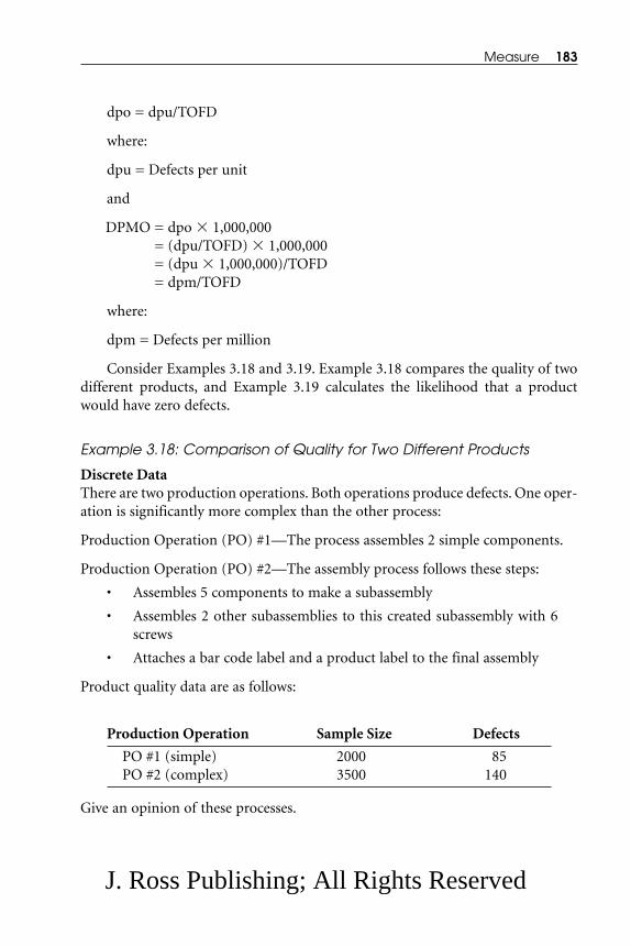
dpo = dpu/TOFD
where:
dpu = Defects per unit
and
DPMO = dpo � 1,000,000= (dpu/TOFD) � 1,000,000= (dpu � 1,000,000)/TOFD= dpm/TOFD
where:
dpm = Defects per million
Consider Examples 3.18 and 3.19. Example 3.18 compares the quality of twodifferent products, and Example 3.19 calculates the likelihood that a productwould have zero defects.
Example 3.18: Comparison of Quality for Two Different Products
Discrete DataThere are two production operations. Both operations produce defects. One oper-ation is significantly more complex than the other process:
Production Operation (PO) #1—The process assembles 2 simple components.
Production Operation (PO) #2—The assembly process follows these steps:
• Assembles 5 components to make a subassembly
• Assembles 2 other subassemblies to this created subassembly with 6screws
• Attaches a bar code label and a product label to the final assembly
Product quality data are as follows:
Production Operation Sample Size Defects
PO #1 (simple) 2000 85PO #2 (complex) 3500 140
Give an opinion of these processes.
Measure 183
J. Ross Publishing; All Rights Reserved

184 Six Sigma Best Practices
Table 3.18. Discrete Process Sigma Conversion Table
Process Defects Defects Defects Defects DefectsLong-Term Sigma per per per per per
Yield (%) (ST) 1,000,000 100,000 10,000 1,000 100
99.99966 6.0 3.4 0.34 0.034 0.0034 0.00034
99.9995 5.9 5 1 0.05 0.005 0.0005
99.9992 5.8 8 1 0.08 0.008 0.0008
99.9985 5.7 15 1 0.15 0.015 0.0015
99.998 5.6 20 2 0.2 0.02 0.002
99.997 5.5 30 3 0.3 0.03 0.003
99.996 5.4 40 4 0.4 0.04 0.004
99.993 5.3 70 7 0.7 0.07 0.007
99.99 5.2 100 10 1 0.1 0.01
99.985 5.1 150 15 1.5 0.15 0.015
99.977 5.0 230 23 2.3 0.23 0.023
99.967 4.9 330 33 3.3 0.33 0.033
99.952 4.8 480 48 4.8 0.48 0.048
99.932 4.7 680 68 6.8 0.68 0.068
99.904 4.6 960 96 9.6 0.96 0.096
99.865 4.5 1,350 135 13.5 1.35 0.135
99.814 4.4 1,860 186 18.6 1.86 0.186
99.745 4.3 2,550 255 25.5 2.55 0.255
99.654 4.2 3,460 346 34.6 3.46 0.346
99.534 4.1 4,660 466 46.6 4.66 0.466
99.379 4.0 6,210 621 62.1 6.21 0.621
99.181 3.9 8,190 819 81.9 8.19 0.819
98.93 3.8 10,700 1,070 107 10.7 1.07
98.61 3.7 13,900 1,390 139 13.9 1.39
98.22 3.6 17,800 1,780 178 17.8 1.78
97.73 3.5 22,700 2,270 227 22.7 2.27
97.13 3.4 28,700 2,870 287 28.7 2.87
96.41 3.3 35,900 3,590 359 35.9 3.59
95.54 3.2 44,600 4,460 446 44.6 4.46
94.52 3.1 54,800 5,480 548 54.8 5.48
J. Ross Publishing; All Rights Reserved

Measure 185
Table 3.18. Discrete Process Sigma Conversion Table (Continued)
Process Defects Defects Defects Defects DefectsLong-Term Sigma per per per per per
Yield (%) (ST) 1,000,000 100,000 10,000 1,000 100
93.32 3.0 66,800 6,680 668 66.8 6.68
91.92 2.9 80,800 8,080 808 80.8 8.08
90.32 2.8 96,800 9,680 968 96.8 9.68
88.5 2.7 115,000 11,500 1,150 115 11.5
86.5 2.6 135,000 13,500 1,350 135 13.5
84.2 2.5 158,000 15,800 1,580 158 15.8
81.6 2.4 184,000 18,400 1,840 184 18.4
78.8 2.3 212,000 21,200 2,120 212 21.2
75.8 2.2 242,000 24,200 2,420 242 24.2
72.6 2.1 274,000 27,400 2,740 274 27.4
69.2 2.0 308,000 30,800 3,080 308 30.8
65.6 1.9 344,000 34,400 3,440 344 34.4
61.8 1.8 382,000 38,200 3,820 382 38.2
58 1.7 420,000 42,000 4,200 420 42
54 1.6 460,000 46,000 4,600 460 46
50 1.5 500,000 50,000 5,000 500 50
46 1.4 540,000 54,000 5,400 540 54
43 1.3 570,000 57,000 5,700 570 57
39 1.2 610,000 61,000 6,100 610 61
35 1.1 650,000 65,000 6,500 650 65
31 1.0 690,000 69,000 6,900 690 69
28 0.9 720,000 72,000 7,200 720 72
25 0.8 750,000 75,000 7,500 750 75
22 0.7 780,000 78,000 7,800 780 78
19 0.6 810,000 81,000 8,100 810 81
16 0.5 840,000 84,000 8,400 840 84
14 0.4 860,000 86,000 8,600 860 86
12 0.3 880,000 88,000 8,800 880 88
10 0.2 900,000 90,000 9,000 900 90
8 0.1 920,000 92,000 9,200 920 92
J. Ross Publishing; All Rights Reserved
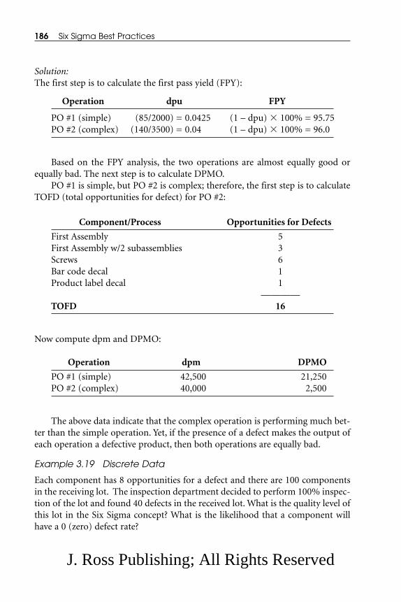
Solution:The first step is to calculate the first pass yield (FPY):
Operation dpu FPY
PO #1 (simple) (85/2000) = 0.0425 (1 – dpu) � 100% = 95.75PO #2 (complex) (140/3500) = 0.04 (1 – dpu) � 100% = 96.0
Based on the FPY analysis, the two operations are almost equally good orequally bad. The next step is to calculate DPMO.
PO #1 is simple, but PO #2 is complex; therefore, the first step is to calculateTOFD (total opportunities for defect) for PO #2:
Component/Process Opportunities for Defects
First Assembly 5First Assembly w/2 subassemblies 3Screws 6Bar code decal 1Product label decal 1
————TOFD 16
Now compute dpm and DPMO:
Operation dpm DPMO
PO #1 (simple) 42,500 21,250PO #2 (complex) 40,000 2,500
The above data indicate that the complex operation is performing much bet-ter than the simple operation. Yet, if the presence of a defect makes the output ofeach operation a defective product, then both operations are equally bad.
Example 3.19 Discrete Data
Each component has 8 opportunities for a defect and there are 100 componentsin the receiving lot. The inspection department decided to perform 100% inspec-tion of the lot and found 40 defects in the received lot. What is the quality level ofthis lot in the Six Sigma concept? What is the likelihood that a component willhave a 0 (zero) defect rate?
186 Six Sigma Best Practices
J. Ross Publishing; All Rights Reserved

Solution: Let,
n = Number of components in the receiving lot
o = Number of defect opportunities per component
d = Total number of defects per receiving lot
DPO = Defects per opportunities
DPMO = Defects per million opportunities
DPO = d/(n � o)
= 40/(100 � 8)
= 0.05
DPMO = DPO � 1,000,000
= 0.05 � 1,000,000
= 50,000
See Table 3.18 (Discrete Process Sigma Conversion Table) for the Sigma value(ST) = 3.15. Under the column entitled Defects per 1,000,000, check for the valueequal to 50,000. There are two nearest values in the column 44,600 and 54,800.Moving horizontally to the reader’s left, the next column is Process Sigma (ST) andthe respective values for 44,600 and 54,800 are 3.2 and 3.1. Therefore, interpolatethe Process Sigma (ST) value for 50,000 (defects) and the Sigma value is 3.15:
• Probability that the opportunity is not defective:= 1 – 0.05= 0.95
• Likelihood that any component will contain zero defects:= (0.95)8
= 0.66= 66%
based on the assumption that 8 opportunities per component are in series. Thisconcept will now be further explained:
Six Sigma series yield concept. Once the components/processes are in series,the system yield decreases as the number of components/processes increases (seeTable 3.19). Table 3.19 shows that if the product has Six Sigma yield metrics (e.g.,Situation 4, which has up to 500 opportunities in series), the product is still yield-ing 99.83% defect-free product. Yet, if the product is in Situation 1, the productquality yield level drops to a very low level in a short time.
Measure 187
J. Ross Publishing; All Rights Reserved

Exercise 3.7: Determining a Single Metric to Compare Incidence ofDefects in Two Processes
The Production Manager is interested in using a single metric to compare theincidence of defects in the chassis assembly operation for their inserter system vs.the digital postage machine assembly operation of their Postage Metering divi-sion. Defects sample data have been collected:
Operation Sample Size Defects
Chassis assembly 400 50Digital postage machine assembly 1500 125
Description of the chassis assembly operation:
• Assemble 150 components to make a subassembly.
• Assemble 70 components to make a table assembly.
• Assemble two subassemblies with 12 bolts.
• Test the chassis assembly.
Description of the digital postage machine assembly operation:
• Assemble 70 components to make the functional subassembly.
• Attach 10 connection harnesses.
188 Six Sigma Best Practices
Table 3.19. Yield Decreases as Series Complexity Increases
Number ofcomponentsor Process Situation 1 Situation 2 Situation 3 Situation 4
Steps (%) (%) (%) (%)
1 93.32 99.38 99.977 99.99966
3 81.27 98.15 99.93 99.99898
8 57.52 95.15 99.82 99.99728
15 35.45 91.09 99.66 99.9949
25 17.76 85.6 99.43 99.9915
50 3.15 73.27 98.86 99.983
100 53.69 97.73 99.966
200 28.83 95.5 99.932
500 4.46 89.14 99.83
System Yield when Components/Processes Are in Series
J. Ross Publishing; All Rights Reserved

• Attach 6 skin parts.
• Test the final assembly.
Assume an equal level of complexity in both assemblies. Analyze the data andmake a recommendation to the Production Manager. Also establish their Sigmaperformance level.
EPMONext is a discussion of EPMO (errors per million opportunities) for a service area.EPMO is a metric for measuring and comparing the performance of distinctadministrative, service, or transactional processes. EPMO quantifies the totalnumber of errors or mistakes produced by a process per million iterations of theprocess. It takes into account the opportunities for that process to have errors ormistakes (TOFE or total opportunities for errors). If an administrative, service, ortransactional process is simple, it should not present too many chances for com-mitting errors or making mistakes. Yet, if a process is complicated, cumbersome,difficult, or not well defined, it may present many chances for errors and mistakes.
EPMO = (epm)/(TOFE)
where:
epm = Errors per million
= epu � 1,000,000
epu = Errors per unit
The advantages of using EPMO vs. epm are that EPMO takes into considera-tion the complexity of the process and the metric lends itself to comparing theperformance of different administrative, service, or transactional processes inregard to their level of difficulty. Generally, an auditing method is used to collectdata from administrative, service, or transactional processes. The collected sam-ple of data should be large enough to calculate the EPMO. This concept utiliza-tion is explained in Example 3.20.
Example 3.20: Utilizing the EPMO Concept
Two types of administrative processes have been audited:• Generation of invoices in the Billing Department• Generation of payroll checks in the Payroll Department
Measure 189
J. Ross Publishing; All Rights Reserved

Both processes are equally complicated. Opportunities for errors in each processare listed:
Invoice Generation Process
Activity/Component Opportunities for Errors
Service/product description 1 Service/product quantity 1 Price/unit of service/product 1Price calculation 1Total service/product price calculation 1Applicable discount calculation 1Net price calculation 1Invoice payment condition(s) 1Customer’s name 1Customer’s address 1Customer’s identification number 1
——— Total 11
Payroll Check Generation Process
Activity/Component Opportunities for Errors
Name 1Address 1Security number 1Work hours 1Overtime hours 1Social Security taxes 1401K withholdings 1Medical and other benefits deduction(s) 1Federal taxes 1State taxes 1Stock options withholding 1Check amount 1Pay period 1
———
Total 13
190 Six Sigma Best Practices
J. Ross Publishing; All Rights Reserved

Both processes have been audited. The results are as follows:
Process Audit Sample Size Defects
Invoice generation 195 10Payroll check generation 500 15
Compute epm, EPMO, and the Sigma performance level.
Solution:For the Invoice Generation Process, the order of calculations would be epm,EPMO, and Sigma performance level:
epm = epu � 1,000,000epu = Number of defects/audited sample size
= 10/195= 0.051282
epm = 0.051282 � 1,000,000= 51,282
EPMO = epm/TOFE
For the Invoice Generation Process, TOFE = 11. Therefore,
EPMO = 51,282/11= 4,662
Now check for the Sigma performance value in Table 3.18 (Discrete ProcessSigma Conversion Table). Under the column entitled Defects per 1,000,000, checkfor the value equal to 4,662. The nearest value in this column is 4,660. Movinghorizontally to the reader’s left, the next column is Process Sigma (ST) and thevalue is 4.1. Therefore, Sigma performance level is 4.1.
Similar calculations have been done for the Payroll Generation Process. Theresults are summarized:
Sigma Process epm EPMO Performance
Invoice generation 51,282 4,662 4.1Payroll check generation 30,000 2,308 4.34
The Payroll Check Generation process is slightly better than the InvoiceGeneration process, but both processes are performing at a low Sigma level.
Measure 191
J. Ross Publishing; All Rights Reserved

Continuous Process Database MetricsThis section will discuss calculating Sigma metrics for the continuous processdatabase.
Assuming the process data have normal distribution, the standard normaldistribution has the mean (μ) = 0, and the variance (σ2) or the standard deviation(σ) = 1, and the area under the density curve is equal to 1. The standard normaldistribution is presented in Figures 3.31A and 3.31B. Any value away from themean is measured in terms of standard deviations. Z is a unit of measure that isequivalent to the number of standard deviations. The Z transformation can beapplied as follows:
Z = (Data point – mean)/(Standard deviation)
This converts any normal distribution to a standard normal distribution.
The normal probability distribution values are presented in Table 3.20. Theprobability values of the distribution can be calculated utilizing Microsoft® Excel(MS Excel) logic Normsdist (Z), and the Z value can be obtained for a given prob-ability value using MS Excel logic Normsinv(Probability Value).
The probability values of a normal distribution can also be calculated utiliz-ing MINITAB software, e.g., for a given Z = 1.96, the probability value from neg-ative infinity to 1.96 is 0.975. Store the Z value in column C1 and use the followinglogic commands in MINITAB to obtain the probability value 0.975:
Calc > Probability Distribution > Normal > select Cumulative Probabilityand Input Column location C1 > OK
Probability value can also be converted to Z value utilizing MINITAB soft-ware, e.g, for a given probability value of 0.975 (from negative infinity to a Zvalue), the Z value is 1.96. Store the probability value 0.975 in column C2 and usethe following logic commands in MINITAB to obtain the Z value equal to 1.96:
Calc > Probability Distribution > Normal > Select Inverse CumulativeProbability and Input Column location C2 > OK
The Sigma metric for the continuous data can be calculated as follows:
1. Identify distribution that represents data.
2. Set defects limits.
3. Calculate yield.
4. Convert yield into Sigma value.
As indicated earlier, process data are assumed to have normal distribution;therefore, the next step is to set defect limits. Customer-driven products/servicesgenerally have specification limit(s). Beyond these limits product/service is con-
192 Six Sigma Best Practices
J. Ross Publishing; All Rights Reserved

sidered defective. These limits may be lower specification limits (LSL) and/orupper specification limits (USL). The process of calculating yield and then con-verting yield into Sigma metrics has been explained with the help of a sample sit-uation presented in Example 3.21.
Example 3.21: Calculating Yield and Then Converting Yield into SigmaMetrics
The Connecticut Truck Manufacturing Company purchases power transmissionshafts from a single supplier. The shaft diameter specifications are 50 mm ± 2 mm.
There are 50 power shafts in the latest lot received. Their measured diametersare as follows:
Measure 193
95.44%
99.74%
μ +1σ +2σ +3σ-3σ -1σ-2σ
68.26%
50%
84.13%
97.72%
99.87%
Z- VALUES: 0 1 2 3
Figure 3.31A. Normal Probability Distribution with σ Values
Figure 3.31B. Normal Probability Distribution with Z Values
J. Ross Publishing; All Rights Reserved

194 Six Sigma Best PracticesTa
ble
3.2
0.
Cum
ulat
ive
Pro
bab
iliti
es o
f th
e N
orm
al P
rob
abili
ty D
istr
ibut
ion
(Are
a U
nder
the
No
rmal
Cur
ve f
rom
Neg
ativ
eIn
finit
y to
Z)
Z0.
000.
010.
020.
030.
040.
050.
060.
070.
080.
09
0.0
0.5
0.50
400.
5080
0.51
200.
5160
0.51
990.
5239
0.52
790.
5319
0.53
59
0.1
0.53
983
0.54
380.
5478
0.55
170.
5557
0.55
960.
5636
0.56
750.
5714
0.57
53
0.2
0.57
926
0.58
320.
5871
0.59
100.
5948
0.59
870.
6026
0.60
640.
6103
0.61
41
0.3
0.61
791
0.62
170.
6255
0.62
930.
6331
0.63
680.
6406
0.64
430.
6480
0.65
17
0.4
0.65
542
0.65
910.
6628
0.66
640.
6700
0.67
360.
6772
0.68
080.
6844
0.68
79
0.5
0.69
146
0.69
500.
6985
0.70
190.
7054
0.70
880.
7123
0.71
570.
7190
0.72
24
0.6
0.72
575
0.72
910.
7324
0.73
570.
7389
0.74
220.
7454
0.74
860.
7517
0.75
49
0.7
0.75
804
0.76
110.
7642
0.76
730.
7704
0.77
340.
7764
0.77
940.
7823
0.78
52
0.8
0.78
814
0.79
100.
7939
0.79
670.
7995
0.80
230.
8051
0.80
780.
8106
0.81
33
0.9
0.81
594
0.81
860.
8212
0.82
380.
8264
0.82
890.
8315
0.83
400.
8365
0.83
89
1.0
0.84
134
0.84
380.
8461
0.84
850.
8508
0.85
310.
8554
0.85
770.
8599
0.86
21
1.1
0.86
433
0.86
650.
8686
0.87
080.
8729
0.87
490.
8770
0.87
900.
8810
0.88
30
1.2
0.88
493
0.88
690.
8888
0.89
070.
8925
0.89
440.
8962
0.89
800.
8997
0.90
15
1.3
0.90
320.
9049
0.90
660.
9082
0.90
990.
9115
0.91
310.
9147
0.91
620.
9177
1.4
0.91
924
0.92
070.
9222
0.92
360.
9251
0.92
650.
9279
0.92
920.
9306
0.93
19
J. Ross Publishing; All Rights Reserved

Measure 195
1.5
0.93
319
0.93
450.
9357
0.93
700.
9382
0.93
940.
9406
0.92
920.
9306
0.93
19
1.6
0.94
520.
9463
0.94
740.
9484
0.94
950.
9505
0.95
150.
9292
0.93
060.
9319
1.7
0.95
543
0.95
640.
9573
0.95
820.
9591
0.95
990.
9608
0.92
920.
9306
0.93
19
1.8
0.96
407
0.96
490.
9656
0.96
640.
9671
0.96
780.
9686
0.92
920.
9306
0.93
19
1.9
0.97
128
0.97
190.
9726
0.97
320.
9738
0.97
440.
9750
0.92
920.
9306
0.93
19
2.0
0.97
725
0.97
780.
9783
0.97
880.
9793
0.97
980.
9803
0.98
080.
9812
0.98
17
2.1
0.98
214
0.98
260.
9830
0.98
340.
9838
0.98
420.
9846
0.98
500.
9854
0.98
57
2.2
0.98
610.
9864
0.98
680.
9871
0.98
750.
9878
0.98
810.
9884
0.98
870.
9890
2.3
0.98
928
0.98
960.
9898
0.99
010.
9904
0.99
060.
9909
0.99
110.
9913
0.99
16
2.4
0.99
180.
9920
0.99
220.
9925
0.99
270.
9929
0.99
310.
9932
0.99
340.
9936
2.5
0.99
379
0.99
400.
9941
0.99
430.
9945
0.99
460.
9948
0.99
490.
9951
0.99
52
2.6
0.99
534
0.99
550.
9956
0.99
570.
9959
0.99
600.
9961
0.99
620.
9963
0.99
64
2.7
0.99
653
0.99
660.
9967
0.99
680.
9969
0.99
700.
9971
0.99
720.
9973
0.99
74
2.8
0.99
744
0.99
750.
9976
0.99
770.
9977
0.99
780.
9979
0.99
790.
9980
0.99
81
2.9
0.99
813
0.99
820.
9982
0.99
830.
9984
0.99
840.
9985
0.99
850.
9986
0.99
86
3.0
0.99
865
0.99
870.
9987
0.99
880.
9988
0.99
890.
9989
0.99
890.
9990
0.99
90
J. Ross Publishing; All Rights Reserved

51, 50, 52, 50, 49.9, 51.5, 49.9, 50, 51, 50.5, 51.5, 50, 52, 51.5, 52.1, 52, 51.9, 52.1,50, 50, 51, 50.5, 50, 51, 51, 50, 51, 50, 49, 49, 49.5, 48, 49.5, 48.9, 50, 50, 49.5, 48,49.5, 49, 50, 49, 50, 49, 51, 51.5, 49, 49.5, 50, 50
Utilize the MINITAB tool to:
• Develop a histogram with normal curve.
• Run a process capability analysis to see if the supplier is capable ofmeeting the engineering specifications of 50 mm + 2 mm.
Solution: Part 1Enter shaft diameter data in column C1 and use the following commands:
Stat > Basic Statistics > Display Descriptive Statistics > Select variable C1> Click on Graph > Select Histogram of data, with normal curve > OK
A histogram with normal curve will be developed (see Figure 3.32A). Descriptivestatistics are presented in Table 3.21.
Solution: Part 2Now check the process capability of the supplier as per engineering specificationsand use tool commands:
Stat > Quality Tools > Capability Analysis (Normal) > Select variable C1in Single Column > Subgroup size: type 50 > Lower Spec: type 48 > UpperSpec: type 52 > Options > Target (adds CPM to table) 50 > Calculate sta-tistics using: 6.0 Sigma tolerance > OK
The process capability analysis is presented in Figure 3.32B.
196 Six Sigma Best Practices
Table 3.21. Descriptive Statistics for Shaft Diameter
Descriptive Statistics for C1
Variable N Mean Median
C1 50 50.246 50.000
Variable Tr Mean SD SE Mean
C1 50.255 1.054 0.149
Variable Minimum Maximum Q1 Q3
C1 48.000 52.100 49.500 51.000
J. Ross Publishing; All Rights Reserved

Under observed performance, none of the shafts in the sample lot is below theLSL, and 2 shafts of 50 shafts in the sample are above the USL. Once this relation-ship is converted based on 1 million shafts, the number of defective shafts wouldbe 40,000. Therefore, PPM (parts per million) based on the USL is 40,000. Now,looking at Table 3.18, based on 40,000 defects per million, the Sigma metrics valuewould be approximately 3.25.
Continue the concept of continuous data with the assumption of normal dis-tribution. The next step is to calculate Z value, where Z is a unit of measure thatis equivalent to the number of standard deviations a value is away from the meanvalue. If the value of Z is positive, the location is to the right of the mean value; ifthe value of Z is negative, the location is to the left of the mean value. The Z valuecan be calculated as follows:
Z = (Data point – mean value)/(standard deviation)
The value of Z helps to convert any normal distribution to a standard normaldistribution with mean (μ) = 0 and variance (σ2) = 1, N ~ (0,1) and also as N ~(μ, σ2). The product/process yield can be presented as follows:
Yield = 1 – Probability of defect
where yield is the percentage of the defect-free product/service produced. Theyield concept is graphically presented in Figure 3.33.
Assume that the product has USL at Z equal to 2. Therefore,
Measure 197
52.051.551.050.550.049.549.048.548.0
15
10
5
0
C1
Fre
quen
cyHistogram of C1, with Normal Curve
Figure 3.32A. Histogram of C1 with Normal Curve for Shaft Diameter
J. Ross Publishing; All Rights Reserved

• Defect-free product/service = 98% and
• Defective product/service = 2%
Now check the Sigma metrics value in Table 3.18 for a 2% defectiveproduct/service. The Sigma value is approximately 3.55.
So far how to calculate Sigma metrics for discrete and continuous data havebeen discussed. These metrics values are short-term Sigma values. The long-termSigma value for a process may not stay the same as the value that the teamachieved in the short term.
198 Six Sigma Best Practices
5453525150494847
Target USLLSL
PPM Total
PPM > USL
PPM < LSL
PPM Total
PPM > USL
PPM < LSL
PPM Total
PPM > USL
PPM < LSL
Ppk
PPL
PPU
Pp
CpmCpk
CPL
CPU
Cp
StDev (Overall)
StDev (Within)
Sample N
Mean
LSL
Target
USL
65774.20
48816.41
16957.79
65774.20
48816.41
16957.79
40000.00
40000.00
0.00
0.55
0.71
0.55
0.63
0.620.55
0.71
0.55
0.63
1.05890
1.05890
50
50.246
48.000
50.000
52.000
Exp. “Overall” PerformanceExp. “Within” PerformanceObserved Performance
Overall CapabilityPotential (Within) CapabilityProcess Data
Within
Overall
Figure 3.32B. Supplier’s Process Capability Analysis for C1 for Shaft Diameter
J. Ross Publishing; All Rights Reserved

Motorola’s 1.5 Sigma Shift ConceptsThe plus or minus (± 1.5) sigma shift surfaced when Motorola used it as a worst-case scenario of a significant shift in process average in their explanation of WhySix Sigma? Motorola said that a ± 1.5 sigma shift would not be detrimental totheir customers’ out-of-tolerance percentage if Motorola’s processes weredesigned to have their specification limits at twice the process width or at SixSigma levels. This concept is presented in Figure 3.34.
The Six Sigma value of 3.4 PPM (parts per million) is defined in Motorola’sdocument entitled Our Six Sigma Challenge. According this document, if thedesign specifications were twice the process width, the process would be extremelyrobust. Such a process would be robust enough. Even if there were a significantor detrimental shift in average and even if it were as high as +1.5 sigma, a cus-tomer would not perceive degradation in product/service quality. In a worst-casescenario, a shift of 1.5 sigma would make an almost 0 defect product/servicechange to 3.4 PPM. In this case, a customer would only perceive an increase from0 to 3 defects per million. This result was supposed to be the warranty Six Sigmaprocesses brought to customers and not actual PPM levels for Six Sigma.
After a process has been improved using Six Sigma DMAIC methodology, theprocess standard deviation and the Sigma value are calculated. DMAIC projectsand the related data are generally collected over a short-term period rather thanover years. Short-term values generally contain common cause variation.However, long-term data contain common cause variation and special cause vari-ation. Because short-term data generally have no special cause variation, short-
Measure 199
Upper SpecificationLimit (USL)
Probabilityof Defect
Z-Values
Yield
50%
84%
98%
MeanValue
Right SideWith Positive “Z”
Left SideWith Negative “Z”
-2 -1 0 +1 +2
Figure 3.33. Product/Service Yield and Defect Concept
J. Ross Publishing; All Rights Reserved

term data will typically be of a higher process capability than long-term data. Thisdifference is the 1.5 sigma shift. Once enough process data has been collected, thefactor most appropriate for a process can be determined.
Six Sigma concepts are all about improvement. When running processesunder statistical control, the user would rather control the input process variablesthan the usual output product variables. The bottom-line impact of the Six Sigmaprocess is to reduce defects, errors, and mistakes to zero defects. Therefore, theobjective of Six Sigma process improvement is to reduce variation in the prod-uct/process such that the specification limits are at least six standard deviationsaway from the mean.
The concepts of current Sigma metrics, goal Sigma metrics, and the Sigmashift are now presented together in Example 3.22.
Example 3.22: Current Sigma Metrics, Goal Sigma Metrics, and SigmaShift
The Connecticut Manufacturing Company is currently manufacturing threeproducts—A, B, and C. Their current and goal manufacturing cycle statistics arepresented in Table 3.22. The goal statistics are assumed to be at the short-term SixSigma metrics level.
Current statistics for all products (A, B, and C) are also shown in a histogramformat along with the normal distribution curves (Figures 3.35A, 3.35B, and3.35C). Calculate the current Sigma metrics for all of the products (A, B, and C).
200 Six Sigma Best Practices
-6 S +6 S
+ Six Sigma Design
+ 1.5 S
3.4 PPM 3.4 PPM
Figure 3.34. Sigma Shift—Long-Term vs. Short-Term Data
J. Ross Publishing; All Rights Reserved

Solution: Sigma Metric for Product A The given goal data represent short-term goal statistics. Now, assume the worst-case scenario that the long-term goal statistics may shift by 1.5 σ. Therefore, thelongest acceptable manufacturing cycle time utilizing the goal statistics would be:
= Goal mean + 4.5 (goal standard deviation)= 19.5 + (4.5 � 3.9)= 37.05 days
Now if the current and goal statistics charts are stacked and both charts areconnected with a dashed line, then the left of both distribution curves would beconsidered as the acceptable manufacturing cycle time area in relation to the givengoal (Figure 3.35A). Therefore, calculate the acceptable normal curve area to theleft of the dashed line in the current manufacturing cycle curve. Now treat thiscalculated area as a Long-Term Yield value in Table 3.18 and find the correspon-ding value in the next column Process Sigma (ST). The value obtained in theProcess Sigma (ST) column would be the current Sigma metric for the manufac-turing cycle of Product A. Calculation steps are as follows:
Step 1. Calculate the Z score for the current manufacturing cycle at 37.05 days.This is an acceptable limit of the goal manufacturing cycle:
Z = (37.05 – 30.78)/11.33= 0.5534
Step 2. Find the probability value at 0.5534 Z from Table 3.20. This value can alsobe obtained through an MS Excel spread sheet as follows:
NORMSDIST(0.5534) = 0.710005
Step 3. The probability value obtained in Step 2 would be used in the Long-TermYield column of Table 3.18. Then find the corresponding value in the Process
Measure 201
Table 3.22. The Current and the Goal Manufacturing Cycle Statistics forProducts A, B, and C
SampleProduct Size (N) Mean SD Mean SD
A 37 30.8 11.33 19.5 3.9
B 34 47.82 21.07 33.0 7.33
C 28 30.32 14.95 23.0 4.5
Manufacturing Cycle (Days)
Current Statistics Goal Statistics
J. Ross Publishing; All Rights Reserved
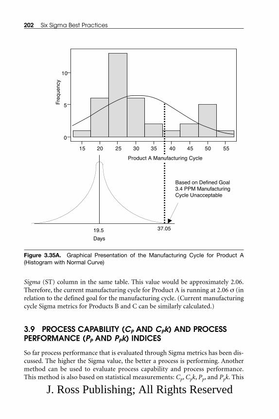
Sigma (ST) column in the same table. This value would be approximately 2.06.Therefore, the current manufacturing cycle for Product A is running at 2.06 σ (inrelation to the defined goal for the manufacturing cycle. (Current manufacturingcycle Sigma metrics for Products B and C can be similarly calculated.)
3.9 PROCESS CAPABILITY (CP AND CPk) AND PROCESSPERFORMANCE (PP AND PPk) INDICES
So far process performance that is evaluated through Sigma metrics has been dis-cussed. The higher the Sigma value, the better a process is performing. Anothermethod can be used to evaluate process capability and process performance.This method is also based on statistical measurements: Cp, Cpk, Pp, and Ppk. This
202 Six Sigma Best Practices
15 20 25 30 35 40 45 50 55
0
5
10
Product A Manufacturing Cycle
Freq
uenc
y
19.5
Days
37.05
Based on Defined Goal3.4 PPM ManufacturingCycle Unacceptable
Figure 3.35A. Graphical Presentation of the Manufacturing Cycle for Product A(Histogram with Normal Curve)
J. Ross Publishing; All Rights Reserved

Measure 203
9080706050403010 20
0
5
10
Freq
uenc
y
Product C Manufacturing Cycle
Figure 3.35C. Graphical Presentation of the Manufacturing Cycle for Product C(Histogram with Normal Curve)
0
5
10
Freq
uenc
y
140120100806040200
Product B Manufacturing Cycle
Figure 3.35B. Graphical Presentation of the Manufacturing Cycle for Product B(Histogram with Normal Curve)
J. Ross Publishing; All Rights Reserved

section will provide a brief discussion of their definitions, interpretations, andcalculations.
Process Capability (CP and CPk) IndexTwo key indices (Cp and Cpk) are used related to technical process capability. Theyare seldom used in administrative service or transactional processes.
CapabilityCapability is defined as the ability of a process to produce product/service withindefined specification limits.
Process Potential Index (CP)The process potential index measures the potential capability of a process. Cp isdefined as the ratio of the allowable spread over the actual spread. This concept ispresented in Figure 3.36:
Cp = (Allowable spread/Actual spread)
Cp = (USL – LSL)/6s
where:
LSL = Lower specification limit
USL = Upper specification limit
204 Six Sigma Best Practices
μActual
LSL USL
Allowable
Figure 3.36. Conceptual Presentation of Cp
J. Ross Publishing; All Rights Reserved
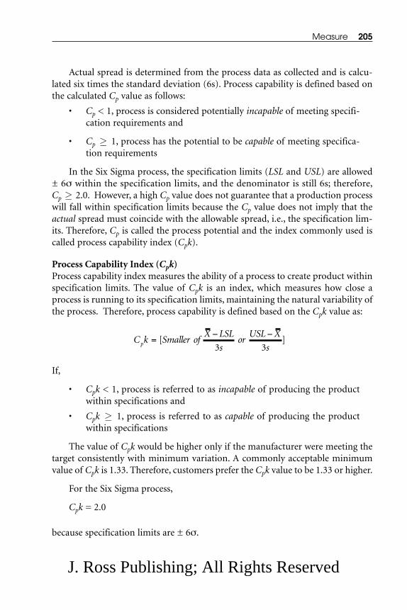
Actual spread is determined from the process data as collected and is calcu-lated six times the standard deviation (6s). Process capability is defined based onthe calculated Cp value as follows:
• Cp < 1, process is considered potentially incapable of meeting specifi-cation requirements and
• Cp ≥ 1, process has the potential to be capable of meeting specifica-tion requirements
In the Six Sigma process, the specification limits (LSL and USL) are allowed± 6σ within the specification limits, and the denominator is still 6s; therefore,Cp ≥ 2.0. However, a high Cp value does not guarantee that a production processwill fall within specification limits because the Cp value does not imply that theactual spread must coincide with the allowable spread, i.e., the specification lim-its. Therefore, Cp is called the process potential and the index commonly used iscalled process capability index (Cpk).
Process Capability Index (Cpk)Process capability index measures the ability of a process to create product withinspecification limits. The value of Cpk is an index, which measures how close aprocess is running to its specification limits, maintaining the natural variability ofthe process. Therefore, process capability is defined based on the Cpk value as:
If,
• Cpk < 1, process is referred to as incapable of producing the productwithin specifications and
• Cpk ≥ 1, process is referred to as capable of producing the productwithin specifications
The value of Cpk would be higher only if the manufacturer were meeting thetarget consistently with minimum variation. A commonly acceptable minimumvalue of Cpk is 1.33. Therefore, customers prefer the Cpk value to be 1.33 or higher.
For the Six Sigma process,
Cpk = 2.0
because specification limits are ± 6σ.
C k Smaller ofX LSL
sor
USL X
sp [ ]=− −3 3
Measure 205
J. Ross Publishing; All Rights Reserved

The higher the Cpk, the narrower the process distribution is, as compared tothe specification limits, and the more uniform the product is. As standard devia-tion increases, the Cpk index decreases, which creates the potential to produceproduct outside the specification limits. Cpk has only positive values.
When Cpk = 0, the actual process average matches or falls outside one of thespecification limits. The Cpk value will never be greater than Cp, only equal to itwhen the actual process falls in the middle of specification limits.
Parts per million (PPM) is another process quality metric. PPM applies to:
• Defective product or part (component)
• Defects
• Errors
• Mistakes
Therefore, the metrics can be linked as follows:
• Defects per million
• Errors per million
• Mistakes per million
• Defectives per million
• PPM defective
The standard values for Cp, Cpk, and PPM for ± Xσ (Sigma levels) are pre-sented in Table 3.23 (if the product/service data are normally distributed with sta-bility and distribution centered).
Process Performance (Pp) and Process Performance Index (Ppk)Process performance (Pp) is a simple indicator of the actual process performance,while the process performance index (Ppk) simply tries to verify whether or notthe collected sample from the process would meet the specification limits. Thelogic used to calculate Ppk is the same as that used for Cpk, except that Cpk uses theestimated sigma (s) and Ppk uses the calculated sigma (sc). Therefore,
If,
• Ppk < 1, actual process is incapable of producing the product withinspecification limits and
P k Smaller ofX LSL
sor
USL X
sp
c c
=− −
[ ]3 3
206 Six Sigma Best Practices
J. Ross Publishing; All Rights Reserved

• Ppk ≥ 1, actual process is capable of producing the product withinspecification limits
For the Six Sigma process,
Ppk = 2.0
because specification limits are ± 6σ.
Differences between Cpk and Ppk. Identified differences between Cpk and Ppkinclude:
• The value of Cpk is for the short-term; the value of Ppk is for the long-term.
• Cpk references the variation to the specification limits, while Ppk pro-duces an index number for the process variation.
• Cpk can be used to determine how process variation would affect theability of the process to meet customer needs/requirements (CTQs),while the Ppk measurement would be used to answer, “How muchvariation is in the process.”
• Cpk presents the future capability of the process, assuming that theprocess remains in a state of statistical control; although Ppk presentspast process performance, it cannot be used to predict the future.
• The values of Cpk and Ppk will converge to almost the same valuewhen the process is in statistical control, i.e., both the standard devi-ations (estimated and calculated) are identical. However, when thestandard deviations are distinctly different, the process is out ofcontrol.
Measure 207
Table 3.23. Sample Values for Cp, Cpk, and PPM
Standard Condition Cp Cpk PPM
[± 1 σ] ≅ one sigma 0.33 0.33 317,320
[± 2 σ] ≅ two sigma 0.67 0.67 45,500
[± 3 σ] ≅ three sigma 1.0 1.0 2,700
[± 4 σ] ≅ four sigma 1.33 1.33 63.5
[± 4.5 σ] ≅ four and a half sigma 1.50 1.50 6.9
[± 5 σ] ≅ five sigma 1.67 1.67 0.6
[± 6 σ] ≅ six sigma 2.0 2.0 0.002
J. Ross Publishing; All Rights Reserved

3.10 SUMMARY
In this chapter, a discussion of the Measure phase of the DMAIC process has beenpresented with key topics:
• Definition of Measure
• Data type
• Data dimension and qualification
• Closed-loop data measurement system
• Flow charting
• Business metrics
• Cause-and-effect diagram
• Failure mode and effects analysis (FMEA) and failure mode, effects,and criticality analysis (FMECA)
• Data collection plan
• Data presentation plan (tables, charts, graphs, and basic statistics)
• Introduction to MINITAB tool
• Determining sample size
• Probabilistic data distributions (normal, Poisson, exponential, bino-mial, gamma, and Weibull)
• The Central Limit Theorem
• Calculating sigma (discrete and continuous data processes):
– Defects per million opportunities (DPMO)
– Errors per million opportunities (EPMO)
– Sigma shift (long term vs. short term)
• Process capability indices
A project team must perform the following tasks before proceeding toAnalyze, the next phase of the DMAIC process:
• Ensure completion of:
– Selection and team approval of key measures
– A data collection plan (with a decision made that historical datacan be utilized or that data collection is needed)
– Accounting for long- and short-term process variability
– Baseline process performance in Sigma metrics
• Identify the following factors:
208 Six Sigma Best Practices
J. Ross Publishing; All Rights Reserved

– Input variables, process variables, and output variables
– Key measures to identify business performance
– Customer CTQs, defect opportunities, and process capabilitymetric
– Charts and processes used for display and communication ofprocess variation
– Gap between current performance and the customer-specifiedperformance
– Any “low-hanging fruit” (i.e., any product/process improvementthat is obvious based on preliminary information and which iseasy to implement) for immediate remedies to reduce the gap
– Handy quality tool(s) to get through the Measure phase
REFERENCES
1. Umble, M. and M.L. Srikanth. 1996. Synchronous Manufacturing,Chapter 2. Guilford, CT: Spectrum Publishing.
2. Society of Automotive Engineers/Reliability, Maintainability,Supportability and Logistics Committee. 1993 Jun 18. The FMECAProcess in the Concurrent Engineering (CE) Environment.Aerospace Information Report AIR4845. Available at:http://www.sae.org/technical/standards/AIR4845.
3. Society of Automotive Engineers. 1993. Failure Mode, Effects andCriticality Analysis. Aerospace Recommended Practice, unpublishedpaper. Available at http://www.sae.org/technical/standards/ AIR4845.
4. Bowles, J.B. and R.D. Bonnell. 1997. Failure Mode, Effects, andCriticality Analysis (What It Is and How to Use It). Presented at theAnnual Reliability and Maintainability Symposium, Philadelphia,PA.
5. DOD. 1984 Nov 28. MIL-STD-1629A/Notice 2: Military StandardProcedure for Performing a Failure Mode, Effects and CriticalityAnalysis. Washington, D.C.: U.S. Department of Defense. Availableat http://www.fmeainfocentre.com/download/MILSTD1629.htm.
6. Society of Automotive Engineers. 1994 July. Potential Failure Modeand Effects Analysis in Design (Design FMEA) and forManufacturing and Assembly Process (Process FMEA). InstructionManual. Surface Vehicle Recommended Practice.
Measure 209
J. Ross Publishing; All Rights Reserved

7. Juran, J.M. 2002. Juran Institute’s Transactional BreakthroughStrategy. Southbury, CT: Juran Institute. Chapter 3 (student materialfrom Black Belt certification training class).
8. Hines, W.W. and D.C. Montgomery. 1992. Probability and Statisticsin Engineering and Management Science, Third Edition. New York:John Wiley.
210 Six Sigma Best Practices
This book has free material available for download from theWeb Added Value™ resource center at www.jrosspub.com
J. Ross Publishing; All Rights Reserved
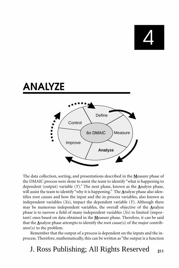
4
ANALYZE
The data collection, sorting, and presentations described in the Measure phase ofthe DMAIC process were done to assist the team to identify “what is happening todependent (output) variable (Y).” The next phase, known as the Analyze phase,will assist the team to identify “why it is happening.” The Analyze phase also iden-tifies root causes and how the input and the in-process variables, also known asindependent variables (Xs), impact the dependent variable (Y). Although theremay be numerous independent variables, the overall objective of the Analyzephase is to narrow a field of many independent variables (Xs) to limited (impor-tant) ones based on data obtained in the Measure phase. Therefore, it can be saidthat the Analyze phase attempts to identify the root cause(s) of the major contrib-utor(s) to the problem.
Remember that the output of a process is dependent on the inputs and the in-process. Therefore, mathematically, this can be written as “the output is a function
211
Define
Measure
Analyze
Improve
Control
J. Ross Publishing; All Rights Reserved

of the inputs and the in-process.” Let X1, X2, . . ., Xn be defined as the inputs andthe in-process and let Y be defined as an output; then, Y = f(X1, X2, X3, . . ., Xn).
The responsibility of a Six Sigma team (a Continuous Improvement team) isto identify the inputs and the in-process (Xs), which are known causes of a seri-ous quality problem(s) that is impacting the output (Y), i.e., the process producesbad/poor-quality output (Y). The team is to find a replacement/modification forthe current input and/or the in-process, implement the recommended improve-ments, and put in place the required controls to maintain the required output.
The collected information from the Measure (measurement) phase generallyprovides potential sources of variation. The team then investigates the variationsand identifies the most critical variations based on the project objectives. Theteam would also utilize individual and/or group experiences as well as availablegraphical/tabular/statistical tools to analyze the information and to “zoom-in” onsources of variation that are impacting team objectives.
So far, the team has been developing theories as to what might be causing theproblem. By testing these theories, root causes will be validated. Using a system-atic approach in the analysis process is important. Therefore, asking the followingquestions before analyzing the information is critical:
• What does the team want to know?
• How should the team view and/or present information?
• Which of the available tools should the team use?
• How and from where did the team get information?
Once the information is processed and analyzed, team should ask anotherquestion:
• As a team, what have we learned?
Next is a brief analysis of these questions.
What Does the Team Want to Know?The team should specifically define goals/objectives and the in-process terms. It isimportant for all team members to participate in the process, e.g., “How do myinput and in-process variables (Xs) affect output (Y)?”
How Should the Team View and/or Present Information?Information can be presented in several ways—descriptively, graphically, and sta-tistically. The team should select the most appropriate way(s) to present informa-tion, e.g., present a population distribution of a town by educational level byusing a pie chart.
212 Six Sigma Best Practices
J. Ross Publishing; All Rights Reserved

Which of the Available Tools Should the Team Use?Utilize the following statements to identify the tools for the information sam-pling, collection, and analyzing plans:
• If the input information can be divided into several categories, utilizemultivariable charts, box plots, and main effects plots for the definedcategories.
• If the input information is continuous, utilize regression/correlationtools. The regression tool develops a prediction equation between thecontinuous input variable and the response variable; the correlationtool provides graphical information about the input variables.
Tool selection depends on the type of information and the way questions arepresented:
• Regression and correlation tool—Energy utilization in material heating
• Box plots, multivariable charts—Employee composition in a com-pany, e.g., by ethnic background
• Pie chart—Relative contribution/composition of a whole, e.g., atown’s population distribution by family
• Control chart—To highlight the average performance and dispersionaround the average, e.g., production data about a shaft diameter
These concepts are also presented in Table 4.1 and Figure 4.1.
How and From Where Did the Team Obtain Information?Typical steps to follow include:
• Identify the input information, e.g., continuous, discrete.
• Develop and explain the plan to team members and all persons whowill participate in information collection and/or analysis.
• If planning to utilize the MINITAB software tool, develop a MINITABinformation entry sheet according to the sampling plan.
• Identify and assign roles and responsibilities for information collec-tion, entry, storage and processing.
• After processing and analyzing the information, ask the next question:“What have we learned?”
What Has the Team Learned?
• Analyze the data using MINITAB software and check the followingpoints/items for completion. These points have been divided into twogroups—question format and statement format. (Some of these
Analyze 213
J. Ross Publishing; All Rights Reserved

points should have been answered based on work previously done.Remaining points will be discussed and answered by the end of thischapter.)
Statement Format Points:
• Identify gaps between the current performance and goal performance.
• Generate list of possible causes (sources of variation).
• Segment and stratify possible causes.
• Prioritize the list of the “vital few” causes.
• Verify and quantify the root causes of variation.
• Determine the performance gap.
• Display and communicate the gap/opportunities in financial terms.
Question Format Points:
• What does the data say about the performance of the businessprocess?
214 Six Sigma Best Practices
Table 4.1. Analysis Tool Selection—Depending on Question and Data Type
Y (Output Variable)
X (Input Variable) Continuous Data Discrete Data
Continuous Data How does change in How does change in input affect change input affect changein output? in output?
Graphical: Scatter plot Statistical: Regression
Statistical: Regression
Discrete Data Different Means? Different Output?
Graphical: Histogram(s) Graphical: StratifiedPareto diagrams
Statistical: t-test, Statistical: FrequencyANOVA counts, chi-square
Different Variance?
Graphical: Stratifiedbox plots, Multivariable
J. Ross Publishing; All Rights Reserved
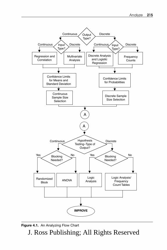
Analyze 215
OutputType?
Continuous Discrete
InputType?
InputType?
Continuous Discrete Continuous Discrete
Regression andCorrelation
MultivariateAnalysis
Discrete Analysisand LogisticRegression
FrequencyCounts
Confidence Limitsfor Means and
Standard Deviation
Confidence Limitsfor Probabilities
ContinuousSample Size
Selection
Discrete SampleSize Selection
A
HypothesisTesting–Type of
Output?
Continuous Discrete
BlockingNeeded?
BlockingNeeded?
Yes NoYes No
RandomizedBlock
ANOVALogic
AnalysisLogic Analysis/
FrequencyCount Tables
IMPROVE
A
Figure 4.1. An Analyzing Flow Chart
J. Ross Publishing; All Rights Reserved

• Did any value-added analysis or “lean thinking” take place to identifysome of the gaps shown on the “as is” process map?
• Was a detailed process map created to amplify critical steps of the “asis” business process?
• How was the map generated, verified, and validated?
• What did the team gain from developing a subprocess map?
• What were crucial “moments of truth” on the map?
• Were any cycle time improvement opportunities identified from theprocess analysis?
• Were any designed experiments used to generate additional insightinto the data analysis?
• Did any additional data need to be collected?
• What model would best explain the behavior of output variables inrelation to input variables?
• What conclusions were drawn from the team’s data collection andanalysis?
• How did the team reach these conclusions?
• What is the cost of poor quality as supported by the team’s analysis?
• Is the process so severely broken that redesign is necessary?
• What are the rough-order estimates of the financial savings/opportu-nity for the improvement project?
• Have the problem and goal statements been updated to reflect theadditional knowledge gained from the Analyze phase?
• Have any additional benefits been identified that will result from clos-ing all or most of the gaps?
• What were the financial benefits resulting from quick fixes (“low-hanging fruits”)?
• What quality tools were used to get through the Analyze phase?
Then,
• State precise and clear conclusions. Update the classified list of inputvariables for repeat or future analysis.
• Design the next study as appropriate.
Discussing all available tools will not be possible in this book; however, com-monly utilized tools will be discussed with examples:
216 Six Sigma Best Practices
J. Ross Publishing; All Rights Reserved

4.1 Stratification
4.2 Hypothesis Testing: Classic Techniques4.2.1 The Mathematical Relationships among Summary Measures4.2.2 The Theory of Hypothesis Testing
4.2.2.1 A Two-Sided Hypothesis4.2.2.2 A One-Sided Hypothesis
4.2.3 Hypothesis Testing—Population Mean and the Differencebetween Two Such Means
4.2.4 Hypothesis Testing—Proportion Mean and the Differencebetween Two Such Proportions
4.3 Hypothesis Testing: The Chi-Square Technique4.3.1 Testing the Independence of Two Qualitative Population
Variables4.3.2 Making Inferences about More than Two Population
Proportions4.3.3 Making Inferences about a Population Variance 4.3.4 Performing Goodness-of-Fit Tests to Assess the Possibility that
Sample Data Are from a Population that Follows a SpecifiedType of Probability Distribution
4.4 Analysis of Variance (ANOVA)
4.5 Regression and Correlation4.5.1 Simple Regression Analysis4.5.2 Simple Correlation Analysis
4.6 Summary
4.1 STRATIFICATION
Stratification is the process of separating data into categories (groups) based ondata variation. A specific combination of ranges or variables defines each data cat-egory. These characteristics are called the stratification variables. Each stratifica-tion variable would have two or more values. One or more variables could bedefined in a category. Data stratification is generally needed to estimate a problemsource in vastly varied information. Yet, in certain conditions, stratification can bemisleading:
• Small differences among groups should not be given undue weight,leading the team to say, “We found it.” The team could prematurelyidentify a cause based on a difference that is insignificant.
Analyze 217
J. Ross Publishing; All Rights Reserved

• An abnormal group of data is not necessarily the cause of a problem.The team should investigate to find the cause and should not maketoo much of abnormal data.
Generally, the following steps should be followed in the stratification process:
• Stratify the data into categories. If additional information needs to becollected, the team has to ensure that all potential stratification vari-ables are collected as identifiers.
• Analyze the categorized data for the likely source of a cause. These cat-egories will be used for each stratification chart/graph. These cate-gories may either be a range of values or discrete values.
• Measure and analyze the significant impact of the phenomenon onthe process.
• Use bar graphs. They are the most effective method for presentingdata. However, other methods are also utilized, e.g., box plots, scatterdiagrams.
If the initial stratification does not provide enough evidence for a cause, theteam has two options:
• Conduct stratification based on the next key variable within the firstvariable.
• Go back and stratify all the data based on some other key variable.
If the team decides that the collected information does not represent theprocess, the team may collect new information. The team should make an effortto collect as much identifying information as they think could possibly prove use-ful for the stratification process. Then the team will go back to the beginning ofthe stratification process and complete the stratification process.
Stratification is an information-analysis tool. The information is analyzedaccording to the stratification factors. A stratification factor is a factor that can beused to separate information into subgroups. Once the team investigates and rec-ognizes a factor as a special cause factor, then that factor is used as a stratificationfactor. If the stratification process is successful, i.e., if the results give a clear indi-cation that more than one group of data exists, then the team should try to vali-date their results or try to gain further information to more precisely define thecause. Additional advantages of stratification include:
• May be used as an initial analysis in the DMAIC process to narrow thescope of the project
• May provide significant help in root-cause analysis
218 Six Sigma Best Practices
J. Ross Publishing; All Rights Reserved

• Because output is a function of input variables, focus is on input variables
• May identify the issue(s) without getting too deeply into the data col-lection and analysis processes
Commonly used stratification elements include:
• Cause Category (type)—Complaints from customer/employee, defec-tive product/process
• Time (when)—Frequency of occurrence (daily, weekly, monthly, etc.)
• Location (where)—Supplier site, customer site, domestic, interna-tional
• Reporting (who)—Individual, group/department, business
Example 4.1 and the Exercise 4.1 will provide a better understanding of strat-ification.
Example 4.1: Using Histograms vs. Box Plots for Analyzing Data
A Connecticut manufacturing company produces three modules (A, B, and C) ofa product. Management is interested in improving the manufacturing cycle time.A Six Sigma team has been selected for the manufacturing cycle time improve-ment project. The team has collected manufacturing cycle time data (Table 4.2A).The project team has also decided to plot a histogram to analyze the cycle time(Figure 4.2A).
As the team analyzed the plotted histogram (Figure 4.2A), the team foundthat the histogram (distribution) had more than one point of concentration, a
Analyze 219
Table 4.2A. Manufacturing Cycle Time Raw Data, Calendar Days
2, 5, 10, 2, 5, 11, 3, 6, 11, 4, 7, 11, 4, 8, 10, 3, 6, 12, 2, 5, 10, 2, 4, 13,
3, 5, 12, 2, 6, 14, 1, 7, 10, 3, 8, 11, 2, 5, 12, 3, 6, 14, 1, 6, 11, 5, 9, 9
Table 4.2B. Manufacturing Cycle Time Data by Module, Calendar Days
Raw Data for Module A, Calendar Days:
2, 2, 3, 4, 4, 3, 2, 2, 3, 2, 1, 3, 2, 3, 1, 5
Raw Data for Module B, Calendar Days:
5, 5, 6, 7, 8, 6, 5, 4, 5, 6, 7, 8, 5, 6, 6, 9
Raw Data for Module C, Calendar Days:
10, 11, 11, 11, 10, 12, 10, 13, 12, 14, 10, 11, 12, 14, 11, 9
J. Ross Publishing; All Rights Reserved

type of distribution known as “multimodal distribution.” (A distribution witha single point of concentration is known as “unimodal distribution.”) Whenmultimodal distribution occurs, likely indicated is that either the data are nothomogeneous or that the data are from more than one source. Therefore, theteam went back and reanalyzed the data and found that all three modules (A,B,
220 Six Sigma Best Practices
1413121110987654321
6
5
4
3
2
1
Manufacturing Days
Sum
of F
requ
ency
Figure 4.2A. Manufacturing Cycle Time Frequency Histogram for All Systems
54321
6
5
4
3
2
1
Manufacturing Days for Module A
Sum
of F
requ
ency
A
Figure 4.2B. Manufacturing Cycle Time Frequency Histogram for Module A
J. Ross Publishing; All Rights Reserved
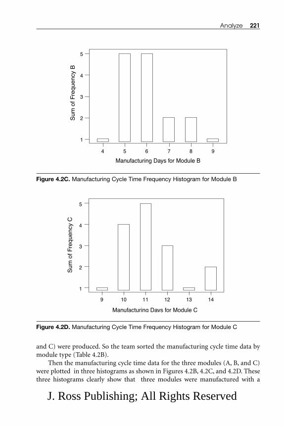
and C) were produced. So the team sorted the manufacturing cycle time data bymodule type (Table 4.2B).
Then the manufacturing cycle time data for the three modules (A, B, and C)were plotted in three histograms as shown in Figures 4.2B, 4.2C, and 4.2D. Thesethree histograms clearly show that three modules were manufactured with a
Analyze 221
987654
5
4
3
2
1
Manufacturing Days for Module B
Sum
of F
requ
ency
B
Figure 4.2C. Manufacturing Cycle Time Frequency Histogram for Module B
14131211109
5
4
3
2
1
Manufacturing Days for Module C
Sum
of F
requ
ency
C
Figure 4.2D. Manufacturing Cycle Time Frequency Histogram for Module C
J. Ross Publishing; All Rights Reserved

manufacturing cycle time range for module A of 1 to 5 days, for module B of 4 to9 days, and for module C of 9 to 14 days.
Assuming that the manufacturing cycle time data of the modules are nor-mally distributed, statistical information has been developed and presented inTable 4.2C and Figures 4.2E and 4.2F. What statistical comments do these figuresand table provide?
Box plots are very similar to histograms. The box plot tool is useful whenworking with small sets of data or when comparing several different sets of data,e.g., the individual modules A, B, and C.
This time, manufacturing cycle time data are plotted utilizing the box plottool (Figure 4.2G) and descriptive statistics are developed (Table 4.2D). Thisinformation should lead to the team deriving the same conclusion as reached ear-lier.
Some definite shortcomings of the stratification process include:
• If small differences exist among the classes of data, a team should notchoose a tool based only on stratification. The team should look forother causes—the category itself is not necessarily the cause.
• If collection of more data is required, the team should give extra effortto identifying information that could be useful in stratification.
222 Six Sigma Best Practices
Table 4.2C. Descriptive Statistics when Combining Manufacturing Cycle for AllModules
Variable N Mean MedianAll Systems 48 6.688 6.000
Variable TrMean SD SE MeanAll Systems 6.614 3.82 0.552
Variable Minimum Maximum Q1 Q3All Systems 1.000 14.000 3.000 10.000
Table 4.2D. Descriptive Statistics by Module (A, B, and C)
Variable Model N Mean Median TrMean SDManufacturing 6 1 6.0000 6.0000 6.0000 *
Cycle A 16 2.625 2.500 2.571 1.088B 15 6.133 6.000 6.077 1.407C 16 11.313 11.000 11.286 1.448
Variable Model SE Mean Minimum Maximum Q1 Q3Manufacturing 6 * 6.0000 6.0000 * *
Cycle A 0.272 1.000 5.000 2.000 3.000B 0.363 4.000 9.000 5.000 7.000C 0.362 9.000 14.000 10.000 12.000
J. Ross Publishing; All Rights Reserved

Analyze 223
151050
6
5
4
3
2
1
0
All Systems Manufacturing Cycle Days Data
Fre
quen
cy
0 5 10 15
All Systems Manufacturing Cycle Days Data
Figure 4.2F. Box Plot for Manufacturing Cycle Time for All Modules
15
10
5
0
Model
Man
ufac
turi
ng C
ycle
Day
s
CBA6
Figure 4.2G. Manufacturing Cycle Time Box Plot by Module ( A, B, and C)
Figure 4.2E. Histogram with Normal Curve for Manufacturing Cycle Frequency for AllModules
J. Ross Publishing; All Rights Reserved

Exercise 4.1: Creating Box Plots for Before and After Data
A Six Sigma quality improvement team has reduced the manufacturing cycle timeof product X. The manufacturing cycle time data are presented in Table 4.3A.Create box plots of the “Before” and “After” data and comment on the team’s qual-ity improvement efforts.
Note: The box plot is provided in Figure 4.3 and descriptive statistics may befound in Table 4.3B if access to the tool is unavailable.
Exercise 4.2: Using the Stratification Tool
Use the stratification tool to investigate the following scenarios. Draw a sketch toshow how output would be viewed:
1. A company has a help desk to resolve hardware and software prob-lems. Employees are complaining that the help desk takes a long
224 Six Sigma Best Practices
Table 4.3A. Manufacturing Cycle Time Datafor Product X Before and After InstallingProcess Improvement
Before After
35 47 30 30
38 46 29 32
37 48 31 29
39 40 32 31
40 42 30 30
42 39 29 29
45 38 31 29
40 41 30 30
Table 4.3B. Descriptive Statistics for Product X Manufacturing Cycle TimeBefore and After Installing Process Improvement
Variable Model N Mean Median TrMean SDModel After 16 30.125 30.000 30.071 1.025Cycle Before 16 41.063 40.000 41.000 3.732
Variable Model SE Mean Minimum Maximum Q1 Q3Model After 0.256 29.000 32.000 29.000 31.000Cycle Before 0.933 35.000 48.000 38.250 44.250
J. Ross Publishing; All Rights Reserved

time to resolve problems. You have been assigned to investigate theemployees’ complaints. Based on preliminary communication, yourtheory is that there may be a time-related element that is creating thelong resolution times. You have collected problem resolution timedata for 4 weeks and are ready to investigate your theory.
2. A company sells preventive maintenance (PM) contracts to cus-tomers who have purchased new equipment. PM services aredivided into four regions (East, West, North, and South). Servicemanagement at your company suspects that the average PM timebetween regions is not the same. You have collected 5 weeks of datafrom all four regions. How would you confirm management’s suspi-cions?
Stratification—The Pareto ChartThe stratification concept can also use a Pareto chart and a cumulative curve. Asample situation is presented in Figure 4.4A. The familiar 80/20 rule (i.e., approx-imately 20% of the problems cause 80% of poor performance) can also be used.The stratification method can also be utilized if an iterative concept is to go moredeeply into a process.
Suppose a company is manufacturing (mostly in an assembly process) fourproducts (A, B, C, and D). These products are manufactured during three shiftoperations (first, second, and third). Each shift operator has a different level ofeducation (less than high school, high school, and higher than high school)(Figure 4.4B). Nine issues (A, B, C, D, E, F, G, H, and I) have been identified.
Analyze 225
50
40
30
Duration
Mod
el C
ycle
After Before
Figure 4.3. Before and After Box Plot for Manufacturing Cycle Time of Product X
J. Ross Publishing; All Rights Reserved

Frequency data for the issues have been collected by operator’s education level. Asample Pareto chart has been developed based on an operator’s education levelbeing below high school (Figure 4.4A). Similar charts can be developed for oper-ators having the two other education levels (a high school education and a higherthan high school education). If these three charts are very similar, then the oper-ator’s education level is not a cause of the frequency of these issues.
226 Six Sigma Best Practices
0
20
40
67
0
50
100
*
*
*
**
** * *
A B C D E F G H I
Issue
Cou
nt
Cum
ulat
ive
Product – A, B, C, D
Assembly Shift – First, Second, Third
Assembly Operator – < HS Education= HS Education> HS Education
Figure 4.4A. Pareto Chart of Manufacturing Issues
Figure 4.4B. Structural Relationship between Products and Operators
J. Ross Publishing; All Rights Reserved

4.2 HYPOTHESIS TESTING: CLASSIC TECHNIQUES
Statistics plays a critical role in Six Sigma projects. Statistical tools identify therelationship between input variables (Xs) and the output variable (Y). The rela-tionship developed in the Analyze phase of the DMAIC process is qualitative. Ifthe qualitative relationship is not strong enough to develop the alternative solu-tions necessary to achieve the project objective(s), then the team has to developthe quantitative relationship. The Design of Experiment (DOE) tool must be uti-lized to develop a quantitative relationship. The DOE tool will be describedChapter 5, Improve. These statistical tools validate the root causes of problems(issues).
Think about the following: every member of the project team has a certainimage of reality in his/her mind; some of these images may be true, while othersmay be false; and all members act accordingly. For example, one team membermay think that wearing a helmet as a safety precaution when driving/riding amotorcycle reduces fatality rates; therefore, we should provide a sales discount forhelmets. Another team member may think that cigarettes cause heart and lungdiseases; therefore, we should increase taxes on cigarettes. Similarly, business peo-ple have other thoughts (beliefs) about certain things and they make importantdecisions everyday based on these beliefs.
Now, consider two scenarios. A sugar manufacturing company packagessugar in 5-pound bags because thought at the company is that this size bag is easyto carry and does not create storage problems. A battery manufacturing companyprovides a battery with an average life of 100 hours because thought at the com-pany is that 100 hours is a good life span for a battery.
In each of these scenarios, and thousands more, people act on the basis oftheir thoughts/beliefs about reality. An initial thought might be in the form of asimple idea, perhaps with a little thought given to it, but with less thought thanwould be done if using informed thinking. This thinking might then become aproposition, which possibly could become true; therefore it can be called ahypothesis. Sooner or later, every hypothesis is tested with evidence that eithersupports or refutes the hypothesis—a process which helps to move a person’simage of reality from great uncertainty to less uncertainty.
Hypothesis testing is a systematic approach to assessing beliefs about reality.Hypothesis testing is confronting a belief (such as test/process data that representan unknown population parameter) with evidence (statistically computed fromthe test/process data) and then deciding, in relation to the collected data, whetherthe initial belief (or hypothesis) can be maintained as reasonable and realistic orif it must be rejected as impractical and insupportable.
Therefore, hypothesis testing is an important concept in a Six Sigma processimprovement program. For example, process team members might want to know
Analyze 227
J. Ross Publishing; All Rights Reserved
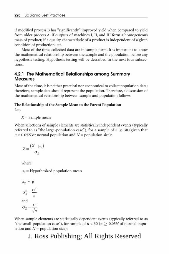
if modified process B has “significantly” improved yield when compared to yieldfrom older process A; if outputs of machines I, II, and III form a homogeneousmass of product; if a quality characteristic of a product is independent of a givencondition of production; etc.
Most of the time, collected data are in sample form. It is important to knowthe mathematical relationship between the sample and the population before anyhypothesis testing. Hypothesis testing will be described in the next four subsec-tions.
4.2.1 The Mathematical Relationships among SummaryMeasuresMost of the time, it is neither practical nor economical to collect population data;therefore, sample data should represent the population. Therefore, a discussion ofthe mathematical relationship between sample and population follows.
The Relationship of the Sample Mean to the Parent Population Let,
⎯X = Sample mean
When selections of sample elements are statistically independent events (typicallyreferred to as “the large-population case”), for a sample of n ≥ 30 (given thatn < 0.05N or normal population and N = population size):
where:
μ0 = Hypothesized population mean
μ⎯X
= μ
and
When sample elements are statistically dependent events (typically referred to as“the small-population case”), for sample of n < 30 (n ≥ 0.05N of normal popu-lation and N = population size):
σσ
Xn
=
σσ
X n2
2
=
ZX
X
=−( )μ
σ0
228 Six Sigma Best Practices
J. Ross Publishing; All Rights Reserved

and
where:
μ⎯X
= Mean of the sampling distribution
σ2
⎯X= Variance of sampling distribution
σ⎯X
= Standard deviation of sampling distribution of the sample mean, ⎯X
while:
μ, σ2, and σ are population mean, variance, and standard deviation, and
N or n are population or sample size, respectively
For the Sampling Distribution of P0
When selections of sample elements are statistically independent events (typicallyreferred to as “the large-population case”), for n < 0.05N:
μp = P
and
When sample elements are statistically dependent events (typically referred toas “the small-population case”), for n ≥ 0.05N:
σ P
P P
n
N n
N0
2 1
1=
−⎛
⎝⎜⎜⎜
⎞
⎠⎟⎟⎟⎟
−−
⎛
⎝⎜⎜⎜
⎞
⎠⎟⎟⎟⎟
( )
sP P
nP0
1=
−( )
σ P
P P
n0
2 1=
−( )
σσ
Xn
N n
N=
−−
( )
( )1
σσ
X n
N n
N2
2
1=
−( )−( )
tX
X
=−( )μ
σ0
Analyze 229
J. Ross Publishing; All Rights Reserved

where:
μp0= Mean of the sampling distribution
σ2p0
= Variance of sampling distribution
σp0 = Standard deviation of sampling distribution of the sample proportion, P0
while:
P is the population proportion and
N and n are population and sample sizes, respectively
The next section (The Theory of Hypothesis Testing) will utilize the above-pre-sented relationship.
4.2.2 The Theory of Hypothesis TestingTo illustrate the testing of hypothesis, consider a game. Let a die be shaken in abox and rolled on a table. If an even number turns up, Player X pays Player Y$1.00. If an odd number turns up, Player Y pays Player X $1.00. Umpire Z doesthe shaking and rolling of the die. If the die is symmetrical and is rolled in a ran-dom manner, the theory of probability tells us that, in the long run, we can expectan equal number of even and odd numbers. Under these conditions, the game willbe a fair one.
Before the game begins, testing the fundamental hypothesis of symmetry andrandomness is desirable. To do this, X and Y agree to have Z roll the die, say, 100times. If the results agree with the expected results, the game will be played asagreed upon; if not, the proper modifications will be made. Of course, the funda-mental question is how close does an agreement with expectations need to bebefore the hypothesis of symmetry and randomness can be accepted?Consideration of this question leads to the theory of hypothesis testing.
In testing a hypothesis, two types of errors may be made:
• To reject a hypothesis when it is actually true—In this case, a type Ierror has been made (also known as Producer’s Risk). With referenceto the illustration, we may conclude after Z rolls the die 100 times, thedie is unsymmetrical or is thrown in a biased manner, when actuallythis is not true.
σ P
P P
n
N n
N0
1
1=
−⎛
⎝⎜⎜⎜
⎞
⎠⎟⎟⎟⎟
−−
⎛
⎝⎜⎜⎜
⎞
⎠⎟⎟⎟⎟
( )
230 Six Sigma Best Practices
J. Ross Publishing; All Rights Reserved

• To accept a hypothesis when it is not true—In this case, a type II errorhas been made (also known as Consumer’s Risk). In this case, we maysay that the die is symmetrical and is thrown in a random manner,when actually it is not.
This situation is presented in Table 4.4. The probabilities of occurrence oftype I and II errors have been given special symbols:
α = P (type I error) = P (reject H0|H0 is true)
β = P (type II error) = P (accept H0|H0 is false)
The Trade-Off Concept of α and βSuppose a null hypothesis is to be tested and definitely unknown is whether thenull hypothesis is true or false. Also unknown is whether the sampling distribu-tion resembles part (a) of Figure 4.5 or part (b) of Figure 4.5. Assuming the sam-pling distribution looks like part (a) of Figure 4.5, and selecting a value of α, adecision rule is developed. This decision rule automatically determines the valueof β if H0 is in fact false. It is clear in Figure 4.5 that for a given sample size, anyreduction in α raises β (as the dashed vertical line moves to the right). The oppo-site is also true: any increase in α lowers β (as the dashed line moves to the left).
Now apply the concept to the sample data statistics presented in Figure 4.5.In part (a) of Figure 4.5, the average paint drying time equals at most 5 hours andis in fact true at a significance level of α = 0.05 and, from the sample, standarddeviation is equal to 0.6 hour. The critical values are ⎯X = 6.0 hours and Z = 1.64.The probability of making a type I error appears to the right of the dashed line.
Part (b) of Figure 4.5 shows the sampling distribution when the null hypoth-esis is in fact false and when the average drying time is 7.18 hours. The criticalvalue of ⎯X = 6 hours (established on the basis of assuming H0 to be true) is nowshown to be lower than the mean value of the sampling distribution, with the cor-responding Z value of –1.96 and the area to the left of this being 0.025. Thisbecomes the probability of making a type II error. Therefore, for any given sam-ple, the selection of α leads to the decision rule and ultimately determines β.
Analyze 231
Table 4.4. Decisions in Hypothesis Testing
H0 is True H0 is False
Accept H0 No error Type II error
Reject H0 Type I error No error
J. Ross Publishing; All Rights Reserved

The Power of the TestSometimes working the power of the test is more convenient, where:
Power = 1 – β = P (reject H0|H0 is false)
The power of the test is the probability that a false null hypothesis is correctlyrejected. Because the results of a test of a hypothesis are subject to error, we can-not “prove” or “disprove” a statistical hypothesis. However, it is possible to designtest procedures that control the error probabilities α and β to suitably small values.
The probability of a type I error is often called the significance level or the sizeof the test. In many tests, α is set at 0.05.
The risk of error of a type II error varies with the actual conditions that existand can be determined by a statistician only as a function of those conditions.Therefore, the chance of saying that the die is symmetrical and is thrown in anunbiased manner, when actually it is either unsymmetrical or is thrown in anunbiased manner, will vary with the degree of a symmetry or bias.
232 Six Sigma Best Practices
α = 0.05
Reject H0 Accept H0
(a) H0 is trueμ ≤ 5 hours
β = 0.025
6.0
Z–1.96 0
5
0
(b) H0 is falseμ = 7.18 hours
6.0
1.64
7.18
Z = ( –X – μ)/σx–
Figure 4.5. Trade-Off between α and β
J. Ross Publishing; All Rights Reserved

The relationship between the chance of accepting a hypothesis and the actualconditions that exist is given by the operating characteristic (OC function) for thetest. Fortunately, statisticians have worked out formulas or derived tables or havefound approximations for the OC functions of many statistical tests, althoughthey are not always in the most desirable form.
Frequently used terms include:
• Null Hypothesis (H0)—This statement is assumed to be true until suf-ficient evidence is presented to reject it. Generally, this statementmeans no change or difference.
• Alternate Hypothesis (H1)—This statement is considered to be true ifH0 is rejected. Generally, this statement means that there is somechange or difference.
• Type I Error—An error (in communication language) that says thereis a difference when actually there is no difference. This is the type oferror that rejects the H0 hypothesis when it is in fact true. In businesslanguage, it can be defined as Producer’s Risk.
• Alpha Risk—The maximum risk or chance of making a type I error.This is the greatest level of risk an analyst (or project team) takes inthe decision-making process when rejecting the H0 hypothesis. Thisprobability is always greater than zero and is normally established at5%.
• Type II Error—An error of not rejecting the H0 hypothesis when it isin fact false. Simply it says that there is no difference when there actu-ally is a difference. In business language, this can be defined asConsumer’s Risk.
• Beta Risk—The maximum risk or chance of making a type II error.Simply, it says that the project team is overlooking an effective processor solution to the problem.
• Significant Difference—Describes the results of a statistical hypothe-sis testing in which the difference is large enough at the defined prob-ability level.
• Power—The probability of correctly rejecting the H0 hypothesis. It isalso utilized to determine if the sample size is large enough to detecta difference in treatments if one exists.
• Test Statistic—Depending on the type of hypothesis testing, the val-ues could be Z, t, F, etc. that represent the feasibility of H0. Generally,the more acceptable the H0, the smaller the absolute value of the test
Analyze 233
J. Ross Publishing; All Rights Reserved

statistic and the greater the probability of observing this value withinits distribution.
Hypothesis testing can be two sided or one sided.
4.2.2.1 A Two-Sided Hypothesis
Remembering the die game, the hypothesis is that the die is symmetrical and thatit is thrown in a random manner or that the probability of an even number is setat 0.5. Therefore, set the risk of an error of the first type (a type I error) at 0.05and let us agree that we shall test the die by rolling it 100 times. Take as the sta-tistic for testing the relative frequency of even numbers in 100 rolls of the die. Ifthe relative frequency falls short of the lower acceptance limit PLa or exceeds theupper acceptance limit PUa, we shall reject the hypothesis; if it equals or fallsbetween these limiting values, we shall accept the hypothesis. First, the quantitiesPLa and PUa have to be determined so that the risk of an error of type I (a) equals0.05.
PLa = p – Zα/2(σP)
PUa = p + Zα/2(σP)
In the die example, p = 0.5, σP = √((0.5 � 0.5)/100) = 0.05, Zα/2 = 1.96.Therefore,
PLa = 0.5 – 1.96(0.05) = 0.402
PUa = 0.5 + 1.96(0.05) = 0.598
In other words, if we get 40 or fewer or 60 or more even numbers from 100rolls of the die, we shall reject the hypothesis of symmetry and unbiased rolling ofthe die. If we get 41 to 59 even numbers, we shall accept the hypothesis.
If we could have the risk of rejecting our hypothesis when it is true at 0.10,then:
PLa = 0.5 – 1.645(σP)
PUa = 0.5 + 1.645(σP)
or we could have made it at 0.01 by taking:
PLa = 0.5 – 2.57(σP)
PUa = 0.5 + 2.57(σP)
234 Six Sigma Best Practices
J. Ross Publishing; All Rights Reserved

4.2.2.2 A One-Sided Hypothesis
Consider a one-tail test applied to an industrial process. Suppose a machiningprocess is producing a component that has historically produced 4% defectivecomponents. The manufacturing process has been modified. Has this modifica-tion lowered the fraction of defective components? To find the answer, test thehypothesis that there has been no change. Use a sample from the current produc-tion process. The setup for the test could be as follows:
• Hypothesis—The current process is operating in a random mannerwith a fraction defective of 0.04.
• Size of Sample—n = 500
• Statistic—The fraction defective in the sample is to be the statisticused in making the test.
• Risk of an Error of the First Type (Type I Error)—Decide to run a riskof 0.05 of rejecting the hypothesis when it is true.
• Acceptance Limits—In this scenario, decide to have only one accept-ance limit Pa, which is less than 0.04. If the sample fraction defectiveis less than Pa, we will reject the hypothesis and conclude that theprocess modification has lowered the process fraction defective. If thesample fraction defective is equal to or greater than Pa, we will acceptthe hypothesis. The quantity Pa is to be determined so that the prob-ability that the sample fraction defective will be less than Pa is just 0.05when the process fraction defective is 0.04.
To determine the acceptance limit Pa, note that the distribution ofsample fraction defective will, because p′ is small, be given approxi-mately by the Poisson distribution, with n = 500 and p′= 0.04. Withthe help of a Poisson distribution chart/table, obtain the expectednumber of defective components. At 500Pa = 20 and p′= 0.04, thevalue from the chart is 13. Therefore, Pa = 13/500 = 0.026. If the sam-ple fraction defective is less than 0.026, we reject the hypothesis thatthe process fraction defective is 0.04.
4.2.3 Hypothesis Testing—Population Mean and the Differencebetween Two Such Means Reminder: Define the problem and state the objectives before establishing thehypothesis.
Next is to state the null hypothesis (H0) and the alternate hypothesis (H1).The hypothesis testing process can be divided into four steps.
Analyze 235
J. Ross Publishing; All Rights Reserved
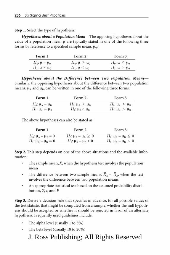
Step 1. Select the type of hypothesis:
Hypotheses about a Population Mean—The opposing hypotheses about thevalue of a population mean μ are typically stated in one of the following threeforms by reference to a specified sample mean, μ0:
Form 1 Form 2 Form 3
H0: μ = μ0 H0: μ ≥ μ0 H0: μ ≤ μ0
H1: μ ≠ μ0 H1: μ < μ0 H1: μ > μ0
Hypotheses about the Difference between Two Population Means—Similarly, the opposing hypotheses about the difference between two populationmeans, μA and μB, can be written in one of the following three forms:
Form 1 Form 2 Form 3
H0: μA = μB H0: μA ≥ μB H0: μA ≤ μB
H1: μA ≠ μB H1: μA< μB H1: μA > μB
The above hypotheses can also be stated as:
Form 1 Form 2 Form 3
H0: μA – μB = 0 H0: μA – μB ≥ 0 H0: μA – μB ≤ 0H1: μA – μB ≠ 0 H1: μA – μB < 0 H1: μA – μB > 0
Step 2. This step depends on one of the above situations and the available infor-mation:
• The sample mean, ⎯X, when the hypothesis test involves the populationmean
• The difference between two sample means, ⎯XA – ⎯XB, when the testinvolves the difference between two population means
• An appropriate statistical test based on the assumed probability distri-bution, Z, t, and F
Step 3. Derive a decision rule that specifies in advance, for all possible values ofthe test statistic that might be computed from a sample, whether the null hypoth-esis should be accepted or whether it should be rejected in favor of an alternatehypothesis. Frequently used guidelines include:
• The alpha level (usually 1 to 5%)
• The beta level (usually 10 to 20%)
236 Six Sigma Best Practices
J. Ross Publishing; All Rights Reserved
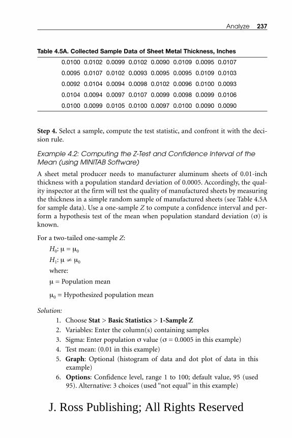
Step 4. Select a sample, compute the test statistic, and confront it with the deci-sion rule.
Example 4.2: Computing the Z-Test and Confidence Interval of theMean (using MINITAB Software)
A sheet metal producer needs to manufacturer aluminum sheets of 0.01-inchthickness with a population standard deviation of 0.0005. Accordingly, the qual-ity inspector at the firm will test the quality of manufactured sheets by measuringthe thickness in a simple random sample of manufactured sheets (see Table 4.5Afor sample data). Use a one-sample Z to compute a confidence interval and per-form a hypothesis test of the mean when population standard deviation (σ) isknown.
For a two-tailed one-sample Z:
H0: μ = μ0
H1: μ ≠ μ0
where:
μ = Population mean
μ0 = Hypothesized population mean
Solution:
1. Choose Stat > Basic Statistics > 1-Sample Z
2. Variables: Enter the column(s) containing samples
3. Sigma: Enter population σ value (σ = 0.0005 in this example)
4. Test mean: (0.01 in this example)
5. Graph: Optional (histogram of data and dot plot of data in thisexample)
6. Options: Confidence level, range 1 to 100; default value, 95 (used95). Alternative: 3 choices (used “not equal” in this example)
Analyze 237
Table 4.5A. Collected Sample Data of Sheet Metal Thickness, Inches
0.0100 0.0102 0.0099 0.0102 0.0090 0.0109 0.0095 0.0107
0.0095 0.0107 0.0102 0.0093 0.0095 0.0095 0.0109 0.0103
0.0092 0.0104 0.0094 0.0098 0.0102 0.0096 0.0100 0.0093
0.0104 0.0094 0.0097 0.0107 0.0099 0.0098 0.0099 0.0106
0.0100 0.0099 0.0105 0.0100 0.0097 0.0100 0.0090 0.0090
J. Ross Publishing; All Rights Reserved

The confidence interval is calculated as follows:
⎯X – Zα/2(σ/√n) to ⎯X + Zα/2(σ/√n)
and
Z = ( ⎯X – μ )/ (σ/√n)
Descriptive statistics for the sample data are presented in Table 4.5B. The dotplot and histogram of the sample data are presented in Figures 4.6A and 4.6B,respectively.
Interpreting the results: The test statistic, Z for testing if the population meanequals 0.0100, is –1.04. Because the P-value of 0.297 is greater than the selected α-value (0.05), there is significant evidence that μ is equal to 0.0100; therefore, weaccept H0 in favor of μ being equal to 0.0100.
Example 4.3: Using the One-Sample t-Test and Confidence Interval
Utilize the sample data from Example 4.2 (see Table 4.5A). Assume that the pop-ulation standard deviation is not known.
Use one-sample t to compute a confidence interval and perform a hypothesistest of the mean when the population standard deviation, σ, is unknown.
For a two-tailed one-sample t:
H0: μ = μ0
H1: μ ≠ μ0
where:
μ = Population mean
μ0 = Hypothesized population mean
238 Six Sigma Best Practices
Table 4.5B. Descriptive Statistics of Sheet Thickness Sample Data—Z Test
One-Sample Z: Sheet Thickness, Inches
Test of mu = 0.01 vs. mu not = 0.01Assumed sigma = 0.0005
Variable N Mean SD SE MeanSheet Thickness 40 0.009918 0.000526 0.000079
Variable 95.0% CI Z PSheet Thickness (0.009763,0.010072) –1.04 0.297
J. Ross Publishing; All Rights Reserved

Analyze 239
Sheet Thickness, Inches
X_
H0
0.009 0.010 0.011
*With Ho and 95% Z-confidence interval for the mean, using sigma = 0.00050000.
][
6
4
2
0
Fre
quen
cy
Sheet Thickness, Inches
X_
H0
*With Ho and 95% Z-confidence interval for the mean, using sigma = 0.00050000.
][
0.00940.00920.0090 0.01000.00980.0096 0.0106 0.01080.01040.0102
Figure 4.6A. Dot Plot of Sheet Thickness Sample Data*
Figure 4.6B. Histogram of Sheet Thickness Sample Data*
J. Ross Publishing; All Rights Reserved

The confidence interval is calculated as follows:
⎯X – tα/2(s/√n) to ⎯X + tα/2(s/√n)
where:
⎯X = Mean of sample data
s = Sample standard deviation
n = Sample size
tα/2 = Value from t-distribution table
where:
α is (1 – confidence level)/100 and degrees of freedom are (n – 1) and
t = ( ⎯X – μ0)/(s/√n)
The descriptive statistics of the sheet thickness sample data are presented inTable 4.5C. See Figure 4.6C for the box plot. (A write-up of the process for thisexample would be the same as for Example 4.2.)
240 Six Sigma Best Practices
0.009 0.010 0.011
Sheet Thickness, Inches
X_
H0
*With Ho and 95% t-confidence interval for the mean.
][
Figure 4.6C. Box Plot of Sheet Thickness Sample Data*
J. Ross Publishing; All Rights Reserved

Interpreting the results: The test statistic, T for H0: μ = 0.0100, is calculatedas –0.99 and the P-value of this test, or the probability of obtaining more extremevalue of the test statistic by chance if the null hypothesis was true, is 0.327. This iscalled the attained significance level (or P-value). Therefore, accept H0 if theacceptable α level (α = 0.05) is lower than the P-value or 0.327.
4.2.4 Hypothesis Testing—Proportion Mean and the Differencebetween Two Such Proportions This process is very similar to the process in Section 4.2.3. Examples will be givenin this section to explain the concept. The following application of a proportionconcept is to compute a confidence interval and perform a hypothesis test. For atwo-tailed test of a proportion:
H0: P = P0 vs. H1: P ≠ P0
where:
P = Population proportion
P0 = Hypothesized value
Data can be in either of two forms: raw or summarized:
• Raw data—All data must be of the same type: numeric, text, ordate/time. (MINITAB default logic defines the lowest value as failureand the highest value as success. This logic can be reversed.)
• Summarized data—Identify the number of trials and one or morevalues for the number of successes. (MINITAB software performs aseparate analysis for each success value.)
Analyze 241
Table 4.5C. Descriptive Statistics of Sheet Thickness Sample Data—T Test
One-Sample T: Sheet Thickness, Inches
Test of mu = 0.01 vs. mu not = 0.01
Variable N Mean SD SE MeanSheet Thickness 40 0.009918 0.000526 0.000083
Variable 95.0% CI T PSheet Thickness (0.009749,0.010086) –0.99 0.327
J. Ross Publishing; All Rights Reserved

Example 4.4: Explaining the Process with MINITAB Software
Utilizing the Summarized Data ConceptA hospital leadership team needs to know if 98% percent of the drug dosages pre-pared by a machine weigh precisely 50 milligrams. A random sample of 500dosages was collected; 485 dosages were found to be of correct weight. Test thehypothesis at a 95% confidence level that the sample represents the expectedmachine performance. Use MINITAB software.
Step 1. Formulate two opposing hypotheses:
H0: P = 0.98H1: P ≠ 0.98
Step 2. Select a test statistic—The standard normal deviate for the sample propor-tion:
where:
P = Observed probability = X/n, where X is the observed number ofsuccesses in n trials
P0= Hypothesized probability
n = Number of trials
Step 3. Derive a decision rule—The expected level of significance is equal to 0.05,where ± Zα/2 = ± 1.96 (because this is a two-tailed test) and the confidence inter-val is:
MINITAB commands:
1. Chose Stat > Basic Statistics > 1 Proportion.
2. Choose Summarized data.
3. In Number of trials, enter 500. In Number of success, enter 485.
4. Click Options.
5. In Test proportion, enter 0.98.
6. From Alternative, choose not equal. Click OK in each dialog box.
A session window output of descriptive statistics is presented in Table 4.6.
ˆˆ ( ˆ )
/P ZP P
n±
−α 2
0 01
ZP P
P P
n
=−( )
−
ˆ
( )
0
0 01
242 Six Sigma Best Practices
J. Ross Publishing; All Rights Reserved

Interpreting the results: The P-value of 0.147 suggests that the data are con-sistent with the null hypothesis (H0: P = 0.98), i.e., the proportion of drug dosagesprepared by the machine is equal to the required proportion of 0.98. The samplerepresents the expected machine performance. Therefore, the null hypothesis canbe accepted.
Testing the Hypothesis and Confidence Interval of Two ProportionsFor a two-tailed test of two proportions:
H0: P1 – P2 = P0 vs. H1: P1 – P2 ≠ P0
where:
P1 and P2 are the proportions of success in populations 1 and 2, respectively
P0 is the hypothesized difference between the two proportions
Data can be in two forms: raw or summarized.
Select the Z statistic for normal distribution assumption. Based on thedefined level of significance, calculate the confidence interval and test the hypoth-esis.
4.3 HYPOTHESIS TESTING: THE CHI-SQUARE TECHNIQUE
Section 4.2 has demonstrated the importance of “normal” distribution and the “t”distribution for purposes of estimating population parameters and/or testinghypotheses about them. In situations when these distributions cannot be used, thechi-square technique is used. Four major applications of the chi-square techniquewill be discussed:
• Testing the independence of two qualitative population variables
• Making inferences about more than two population proportions
Analyze 243
Table 4.6. Descriptive Statistics of Drug Dosages Sample Data
Test and CI for One Proportion
Test of p = 0.98 vs. p not = 0.98
ExactSample X N Sample p 95.0% CI P-Value
1 485 500 0.970000 (0.951002, 0.983114) 0.147
J. Ross Publishing; All Rights Reserved

• Making inferences about a population variance
• Performing goodness-of-fit tests to assess the possibility that sampledata are from a population that follows a specified type of probabilitydistribution
4.3.1 Testing the Independence of Two Qualitative PopulationVariablesGenerally, qualitative variables are not expressed numerically because they differin type rather than in degree among the fundamental units of a statistical popu-lation. Situations are numerous when it is important to know if two such variablesare statistically independent of one another (the probability of occurrence of onevariable is unaffected by the occurrence of the other) or if these variables are sta-tistically dependent (the probability of occurrence of one is affected by the occur-rence of the other). The list of situations would be endless, e.g., the variablesbetween heart attacks and smoking, saturated food intake and cholesterol, systemfailure and prior year of service, customer arrival at a bank and the time of theday, etc.
The procedural steps and an example will follow the mathematical logic ofthe model. Let the observed data be presented in r rows and c columns, creatingthe r × c table; and
Oij = Observed value in cell ij, i = 1, 2, …, r, and j = 1, 2, …, c
Eij = Expected value in cell ij
Then,
Eij = ((Total of row i) × (total of column j))/(total number of observations)
The total χ2 is calculated as follows:
(r –1) × (c – 1) = Degrees of freedom
Steps in the procedure are:
Step 1. State the practical problem and formulate two opposing hypotheses:
H0: The two variables are independent
H1: The two variables are dependent
χ2
2
=−( )
∑∑O E
E
ij ij
ijji
244 Six Sigma Best Practices
J. Ross Publishing; All Rights Reserved

Step 2. Select a test statistic; in this situation:
Step 3. Derive a rule, e.g., needing to set a significance level of α = 0.05 and know-ing degrees of freedom (r – 1)(c – 1), the critical value of χ2
α,df from the chi-squaretable:
“Accept H0 if calc χ2 < table χ2α,df” or
“Reject H0 if calc χ2 > table χ2α,df”
Next, translate the statistical conclusion into process (simple) language (seeExample 4.5).
Example 4.5: Comparing Gender to Soft Drink Consumption
If soft drink consumption is customer-gender related, then different advertise-ments must be created for men’s and women’s magazines. Therefore, a soft drinkproducer wants to know if the gender of consumers is independent of their pref-erences for four brands of soft drinks. A test of independence will be conductedat the 5% significance level based on the sample data presented in Table 4.7A:
Step 1. Formulate two opposing hypotheses:
H0: Gender and soft drink preference are independent variables
H1: Gender and soft drink preference are dependent variables
Step 2. Select a test statistic:
Step 3. Derive a decision rule:
Given: α = 0.05 and 3 degrees of freedom (2 genders and 4 types of soft drink)
Step 4. Select the provided sample data, compute the test statistic, and test it withthe decision rule.
χ2
2
=−( )
∑∑O E
E
ij ij
ijji
χ2
2
=−( )
∑∑O E
E
ij ij
ijji
Analyze 245
J. Ross Publishing; All Rights Reserved

246 Six Sigma Best Practices
Table 4.7A. Sample Data of Soft Drink Preference byGender
Soft Drink Soft DrinkGender Preference Gender Preference
M A M BF A M BF A M BF A M BF A M BF A M BF A M BF B M BF B M BF B M BF C M BF A F C
M A M C
F A F D
M A M C
F A F D
M A M C
F A F D
M A M CF A F DM A M CF A F DM A M CF A M CM A M CF A M D
M A M DF A M DM B M DF A F DF D
J. Ross Publishing; All Rights Reserved

Use MINITAB software to analyze the above data:
1. Open the software and enter the data:
Column C1—Gender
Column C2—Soft drink preference
2. Choose Stat > Table > Cross Tabulation
3. In Classification variable, enter Gender, Soft drink preference
4. Check Chi-Square analysis and then choose Above and std. resid-ual; Click OK
MINITAB output of tabulated statistics for the soft drink preferences by gen-der is presented in Table 4.7B. From the table, χ2
0.05,3 = 7.815.
Interpreting the results: The output data contain the observed frequencycounts, the expected frequencies, and the standardized residual or contribution tothe χ2 statistic, where:
Standard residual = (Observed count – Expected count)/√(Expected count)
The P-value of the test, 0.010, indicates that there is evidence for an associa-tion between the variables Gender and Soft drink preference. Therefore, acceptthe alternate hypothesis:
χ2calculated = 11.45 (see Table 4.7B) and from the chi-square table, χ2
0.05,3 = 7.815
Analyze 247
Table 4.7B. Tabulated Statistics for Soft Drink Preference by Gender
Gender A B C D All
F 16 3 2 7 2811.48 6.89 4.59 5.05 28.00
1.34 –1.48 –1.21 0.87 —
M 9 12 8 4 3313.52 8.11 5.41 5.95 33.00–1.23 1.36 1.11 –0.80 —
All 25 15 10 11 6125.00 15.00 10.00 11.00 61.00
– — — — —
Chi-square = 11.445, df = 3, P-value = 0.010One cell with expected counts less than 5.0
Note: Rows: gender; columns: soft drinks.
J. Ross Publishing; All Rights Reserved
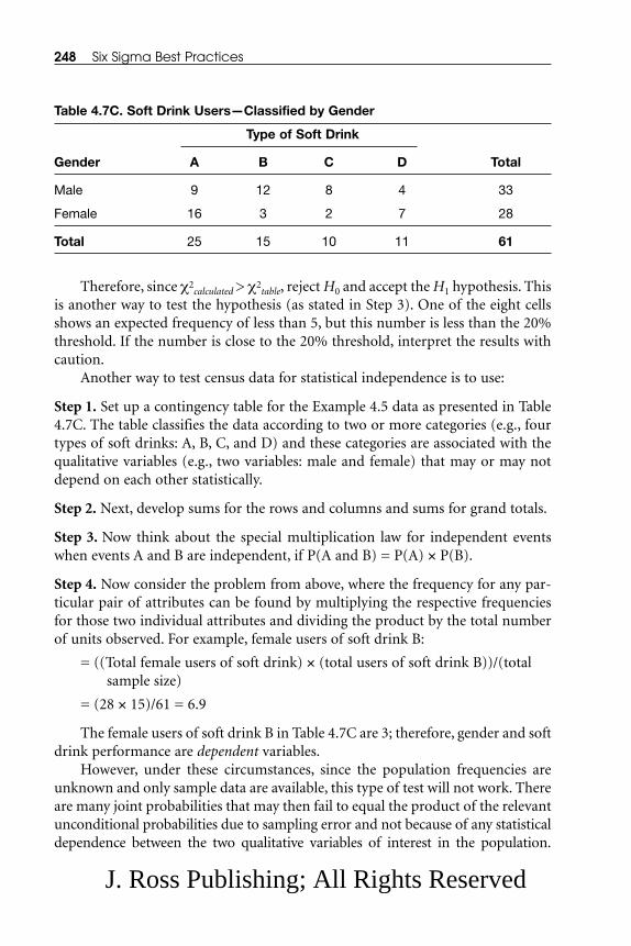
Therefore, since χ2calculated > χ2
table, reject H0 and accept the H1 hypothesis. Thisis another way to test the hypothesis (as stated in Step 3). One of the eight cellsshows an expected frequency of less than 5, but this number is less than the 20%threshold. If the number is close to the 20% threshold, interpret the results withcaution.
Another way to test census data for statistical independence is to use:
Step 1. Set up a contingency table for the Example 4.5 data as presented in Table4.7C. The table classifies the data according to two or more categories (e.g., fourtypes of soft drinks: A, B, C, and D) and these categories are associated with thequalitative variables (e.g., two variables: male and female) that may or may notdepend on each other statistically.
Step 2. Next, develop sums for the rows and columns and sums for grand totals.
Step 3. Now think about the special multiplication law for independent eventswhen events A and B are independent, if P(A and B) = P(A) × P(B).
Step 4. Now consider the problem from above, where the frequency for any par-ticular pair of attributes can be found by multiplying the respective frequenciesfor those two individual attributes and dividing the product by the total numberof units observed. For example, female users of soft drink B:
= ((Total female users of soft drink) × (total users of soft drink B))/(totalsample size)
= (28 × 15)/61 = 6.9
The female users of soft drink B in Table 4.7C are 3; therefore, gender and softdrink performance are dependent variables.
However, under these circumstances, since the population frequencies areunknown and only sample data are available, this type of test will not work. Thereare many joint probabilities that may then fail to equal the product of the relevantunconditional probabilities due to sampling error and not because of any statisticaldependence between the two qualitative variables of interest in the population.
248 Six Sigma Best Practices
Table 4.7C. Soft Drink Users—Classified by Gender
Type of Soft Drink
Gender A B C D Total
Male 9 12 8 4 33
Female 16 3 2 7 28
Total 25 15 10 11 61
J. Ross Publishing; All Rights Reserved

Therefore, under such circumstances the chi-square technique finds its first appli-cation.
4.3.2 Making Inferences about More than Two PopulationProportionsOne effectively assumes that certain proportions (i.e., females among all highschool teachers or males among all taxi drivers) are the same for all categories ofsome variable when expected frequencies are being calculated for the various cellsof a contingency table. The same technique that allows testing for the independ-ence of two qualitative population variables can also be used to test if a numberof population proportions are equal to each other or if they are equal to any pre-determined set of values. The above identified logic will be used in Example 4.6.
Example 4.6: Comparing Integration Line Speeds for PersonalComputers
Consider the process of manufacturing personal computers. Business leaders areinterested in testing the hypothesis that the proportion of defective units (PCs)produced will be the same for each of five possible integration speeds. The qual-ity group at the company has been asked to perform a test at the 1% significancelevel, taking 5 samples of 50 PCs each, while different integration line speeds arebeing maintained. The collected data are presented in Table 4.8A.
The statistical testing process will follow these steps:
Step 1. Formulate two opposing hypotheses:
H0: The population proportion of defectives is the same for each of 5 integra-tion line speeds, i.e., P1 = P2 = P3 = P4 = P5 = 0.05 (given)
H1: The population proportion of defectives is not the same for each of 5 inte-gration line speeds, i.e., at least one of the equalities in H0 does not holdtrue
Analyze 249
Table 4.8A. Collected Sample Data from PC Integration Line
Integration Line Speed (Units per Hour)
PC Quality A = 30 B = 35 C = 40 D = 45 E = 50 Total
(1) Defective 4 5 5 6 7 27
(2) Acceptable 46 45 45 44 43 223
Total 50 50 50 50 50 250
J. Ross Publishing; All Rights Reserved

Step 2. Select a test statistic:
Step 3. Derive a decision rule:
Given: α = 0.01 and 4 degrees of freedom, 2 possible product (PC) qualities, and5 possible integration line speeds:
1 × 4 = 4 df
Step 4. Select the samples, compute the test statistic, and confront it with the deci-sion rule.
Enter the collected sample data need in MINITAB as follows:
A B C D E
4 5 5 6 746 45 45 44 43
1. Choose Stat > Tables > Chi-Square Test.
2. In columns containing the table, enter A B C D E. Click OK.
3. Chi-square test output is presented in Table 4.8B.
From the chi-square table, χ20.01,4 = 13.277
χ2
2
=−( )
∑∑O E
E
ij ij
ijji
250 Six Sigma Best Practices
Table 4.8B. Chi-Square Test Output for Sample Data in Table 4.8A
Chi-Square Test
PC Quality A B C D E Total
(1) 4 5 5 6 7 275.4 5.40 5.40 5.40 5.40
(2) 46 45 45 44 43 22344.60 44.60 44.60 44.60 44.60
Total 50 50 50 50 50 250
Chi-square = 0.363 + 0.030 + 0.030 + 0.067 + 0.474 + 0.044 + 0.004 + 0.004 + 0.008 + 0.057 = 1.080
df = 4; P-value = 0.898
Note: Expected counts are printed below observed counts.
J. Ross Publishing; All Rights Reserved

Interpreting the results: The P-value of 0.898 indicates that there is no strongevidence that the units defective and the integration line speed are related.Therefore, accept the null hypothesis. If a cell had an expected count less than 5,and even with significant P-value for these data, interpret the results with skepti-cism. To be more confident of the results, repeat the test with or without modifi-cations.
4.3.3 Making Inferences about a Population VarianceThe sample variance s2 is an unbiased estimator of the population variance σ2
provided that the selections of sample elements are statistically independentevents. Probabilities of the sample variance can be established with the help of χ2
distributions. Since:
and the converted value in the chi-square with (n – 1) degrees of freedom are asfollows:
where:
s2 = Sample variance
n = Sample size
σ2 = Population variance
and the probability interval for the sample variance, s2:
where:
lower chi-square value and
upper chi-square value
and the confidence interval for the population variance, σ2:
χσU
Us n22
2
1=
−⎛
⎝⎜⎜⎜⎜
⎞
⎠⎟⎟⎟⎟⎟
( )
χσL
Ls n22
2
1=
−⎛
⎝⎜⎜⎜⎜
⎞
⎠⎟⎟⎟⎟⎟
( )
σ χ σ χ2 22
2 2
1 1L U
ns
n−
⎛
⎝⎜⎜⎜⎜
⎞
⎠⎟⎟⎟⎟⎟≤ ≤
−
⎛
⎝⎜⎜⎜⎜
⎞
⎠⎟⎟⎟⎟⎟⎟
χσ
22
2
1=
−s n( )
sX nX
n2
2 2
1=
−−
∑
Analyze 251
J. Ross Publishing; All Rights Reserved

where:
χ2U
= Value of χ2 variable with (n – 1) degrees of freedom such that larger values have a probability of α/2
χ2L
= Value of χ2 variable with (n – 1) degrees of freedom such that smaller values have a probability of α/2
α = 1 – confidence level
As an example, consider a process at a food packing company. The companyis filling bags. The weight of these bags is normally distributed with a populationstandard deviation of σ = 2 ounces (oz). (Therefore, the population variance isσ2 = 4 oz squared). A simple random sample of 25 bags is taken from this popu-lation. Calculate the probability of finding a sample variance between 3 and 5 ozsquared:
Given: s2L
= 3 and s2U
= 5
First calculate χ2L
and χ2U
:
= (3(25 – 1))/4= 18
= (5(25 – 1))/4= 30
Now find the χ2 probability values from the chi-square table for the given χ2
= 18 at 24 degrees of freedom; the probability value is approximately 0.80.Similarly for the calculated χ2 = 30 at 24 degrees of freedom, the probability valueis approximately 0.20. Therefore, the area of about (0.8 – 0.2 = 0.6) lies betweenthese values, and the value of 0.6 is also the probability of finding a sample vari-ance between 3 and 5 oz squared in this example.
Similarly, the limits below and above the specified percentage of all possibles2 values can also be calculated. Take the above example, at 5% each limit (lowerand upper) with 24 degrees of freedom:
χσU
Us n22
2
1=
−⎛
⎝⎜⎜⎜⎜
⎞
⎠⎟⎟⎟⎟⎟
( )
χσL
Ls n22
2
1=
−⎛
⎝⎜⎜⎜⎜
⎞
⎠⎟⎟⎟⎟⎟
( )
s n s n
U L
2
2
22
2
1 1( ) ( )−⎛
⎝⎜⎜⎜⎜
⎞
⎠⎟⎟⎟⎟⎟≤ ≤
−⎛
⎝⎜⎜⎜⎜χ
σχ
⎞⎞
⎠⎟⎟⎟⎟⎟
252 Six Sigma Best Practices
J. Ross Publishing; All Rights Reserved

χ20.95,24 = 13.848 (the lower χ2 value from the chi-square table)
χ20.05, 24 = 36.415 (the upper χ2 value from the chi-square table)
Therefore:
= (4 × 13.848)/(25 – 1)= 2.31
= (4 × 13.415)/(25 – 1)= 6.07
Therefore, 5% of all s2 values would lie below 2.31, another 5% would lieabove 6.07, and 90% would lie between these two values. Next, continue the aboveexample with some modifications:
• New sample size, n = 30 food bags
• Sample variance, s2 = 3 oz squared
What is the 90% confidence interval of σ2?
Since α = 0.10, and degrees of freedom = 29, then from the chi-square table:
χ2U
= χ20.05, 29 = 42.557
χ2L
= χ20.95, 29 = 17.708
and the σ2 interval can be calculated as follows:
2.04 ≤ σ2 ≤ 4.91
Therefore, with 90% confidence, the food bags’ variance can be said to bebetween 2.04 and 4.91 oz squared, and the food bags’ standard deviation isbetween 1.43 and 2.22 oz.
3 30 1
42 557
3 30 1
17 7082( )
.
( )
.
−⎛
⎝⎜⎜⎜
⎞
⎠⎟⎟⎟⎟≤ ≤
−⎛
⎝σ ⎜⎜⎜⎜
⎞
⎠⎟⎟⎟⎟
snU
U22 2
1=
−
⎛
⎝⎜⎜⎜⎜
⎞
⎠⎟⎟⎟⎟⎟
σ χ
snL
L22 2
1=
−
⎛
⎝⎜⎜⎜⎜
⎞
⎠⎟⎟⎟⎟⎟
σ χ
Analyze 253
J. Ross Publishing; All Rights Reserved

Testing the Hypothesis about the Population VarianceThese hypotheses could be one-sided or two-sided, and the one-sided one couldbe a lower-tailed or upper-tailed hypothesis. Three examples present varieties ofthese hypotheses: Example 4.7, a lower-tail hypothesis test; Example 4.8, anupper-tail hypothesis test; and Example 4.9, a two-tail hypothesis test.
Example 4.7: Using a Lower-Tail Hypothesis Test
This lower-tail hypothesis test will use an airline’s booking area waiting-line pol-icy as an example. Airline management would like to introduce the concept of asingle-line policy that directs all passengers to enter a single waiting line in theorder of their arrival and that in turn would direct them to different check-incounters. Airline management thinks a single-line policy will decrease waiting-time variability. However, some critics of management claim that variabilitywould be at least as great with a single-line policy as with a policy of multipleindependent lines, which in the past had a standard deviation of σ0 = 8 minutesper customer checking in. A hypothesis at the 2% significance level is to settle theissue. The hypothesis is to be based on the experience of a random sample of 30customers subjected to the new policy.
Next, formulate two opposing hypotheses:
H0: Single waiting-line’s variance would be equal to or greater than 64minutes squared (σ2 ≥ 64)
H1: Single waiting-line’s variance would be less than 64 minutes squared(σ2 < 64)
and the test statistics:
The concept of deriving the decision policy is presented in Figure 4.7A.
Given: A desired significance level of α = 0.02 and n – 1 = 29 degrees of freedom,value from the chi-square table, χ2
0.98, 29 = 15.574 (this is a lower-tail test)
Therefore, the decision rule must be:
Accept H0 if χ2calculated > 15.574
A sample was collected, test statistics were computed, and the results weretested with the decision rule. After taking a sample of 30 passengers, the standarddeviation was computed and s = 3 minutes. Now compute the test statistic:
χσ
22
02
1=
−⎛
⎝⎜⎜⎜⎜
⎞
⎠⎟⎟⎟⎟⎟
s n( )
254 Six Sigma Best Practices
J. Ross Publishing; All Rights Reserved

= (32)(30 – 1)/64= 4.08
This result suggests that the null hypothesis should be rejected. At a 2% sig-nificance level, the sample result is statistically significant. The observed diver-gence from the hypothesized value of σ0 = 8 minutes is unlikely to be the result ofchance factors operating during sampling. It is more likely to be the result of man-agement being right—a single waiting line feeding into several check-in countersdoes reduce waiting-time variability.
Example 4.8: Using an Upper-Tail Hypothesis Test
This upper-tail hypothesis test will use the variation of a digital postage meter asan example. A manufacturer of postage metering equipment is bringing out a newmodel of a digital meter (the meter is used for weighing an envelope, calculatingpostage, and stamping the calculated postage on the envelope). The standarddeviation of the postage calculation on the old model was σ0 = 0.5 cents. Ahypothesis test at the 5% significance level is to be conducted to support the man-ufacturer’s claim that the new meter’s variability is equal to or less than that of theold model. The test involves collecting 25 readings from known postage require-ments.
Formulate two opposing hypotheses:
H0: New digital postage meter variance would be equal to or less than 0.25cents squared (σ2 ≤ 0.25)
H1: New digital postage meter variance would be greater than 0.25 centssquared (σ2 > 0.25)
χσ
22
02
1=
−⎛
⎝⎜⎜⎜⎜
⎞
⎠⎟⎟⎟⎟⎟
s n( )
Analyze 255
FrequencyDensity
α = 0.02
df = 29
χ2 0
Reject H0 Accept H0
χ20.98, 29 = 15.574
Figure 4.7A. Hypothesis Testing Decision Rule (Lower-Tail Test)
J. Ross Publishing; All Rights Reserved

and the test statistics:
The concept of deriving the decision policy has been presented in Figure 4.7B.
Given: A desired significance level of α = 0.05 and (n – 1) = 24 degrees of free-dom, value from the chi-square table, χ2
0.05, 24 = 36.415 (this being anupper-tail test)
Therefore, the decision rule must be:
Accept H0 if χ2calculated ≤ 36.415
A sample was collected, test statistics were computed, and the results weretested with the decision rule. After taking a sample of 25 postage meter stampingreadings, the standard deviation was calculated and s = 0.3 cents.
Now compute the test statistic:
= (0.32 (25 – 1))/0.52= 8.64
This result suggests that the null hypothesis should be accepted. At the 5%significance level, the sample result is statistically insignificant. The new digitalpostage meter is equal to or better than the old one as claimed by the manufac-turer.
χσ
22
02
1=
−⎛
⎝⎜⎜⎜⎜
⎞
⎠⎟⎟⎟⎟⎟
s n( )
χσ
22
02
1=
−⎛
⎝⎜⎜⎜⎜
⎞
⎠⎟⎟⎟⎟⎟
s n( )
256 Six Sigma Best Practices
FrequencyDensity
α = 0.05
df = 24
χ20
Reject H0Accept H0
χ20.05, 24 = 36.415
Figure 4.7B. Hypothesis Testing Decision Rule (Upper-Tail Test)
J. Ross Publishing; All Rights Reserved

Example 4.9: Using a Two-Tail Hypothesis Test
This two-tail hypothesis test will use the diameter of a fuel tank lid in an aircraftas an example. An aircraft manufacturer is concerned about the variability in thelid diameter for a lid that is used to seal the fuel system. The fuel system is locatedinside the aircraft’s wings. Only a narrow range of lid diameter is acceptable. If thelid fits too tightly, the lid will prevent air from entering the fuel system as the fuelis being consumed, creating a vacuum and ultimately causing the wing structureto collapse. A lid that fits too loosely can allow fuel to be sucked out of the fuelsystem during flight, which is equally undesirable for flight safety. Therefore, a testat the 2% significance level is to be conducted with a random sample of 30 fuelsystem lids to see if the variance of lid diameters is equal to 0.0001 inch squaredas specified by designers.
Formulate two opposing hypotheses:
H0: Fuel system’s lid diameter variance would be equal to 0.0001 inchsquared (σ2 = 0.0001)
H1: Fuel system’s lid diameter variance would not be equal to 0.0001 inchsquared (σ2 ≠ 0.0001)
and the test statistics:
The concept of deriving the decision policy is presented in Figure 4.7C.
χσ
22
02
1=
−⎛
⎝⎜⎜⎜⎜
⎞
⎠⎟⎟⎟⎟⎟
s n( )
Analyze 257
FrequencyDensity
α/2 = 0.01
df = 29
χ2
Reject H0 Reject H0Accept H0
χ20.99, 29 = 14.953
α/2 = 0.01
χ20.01, 29 = 50.892
Figure 4.7C. Hypothesis Testing Decision Rule (Two-Tail Test)
J. Ross Publishing; All Rights Reserved
Given: A desired significance level of α = 0.02 and a two-tail test; the lower andthe upper critical χ2 values must be established (0.01 of the area under theχ2 distribution lies below and above each of these values)
Therefore, the values from the chi-square table:
χ20.99, 29 = 14.953 and χ2
0.01, 29 = 50.892
The decision rule must be:
Accept H0 if 14.953 ≤ χ2 ≤ 50.892
A sample of 30 lids was collected, test statistics were computed, and the resultswere tested with the decision rule. The calculated standard deviation was s = 0.01inch, and the computed value of the test statistic equals:
= ((0.01)2 (30 – 1)) / 0.0001= 29
This result suggests that the null hypothesis should be accepted. At the 2%significance level, the sample result is not statistically significant. Therefore, thefuel system lids meet specifications.
4.3.4 Performing Goodness-of-Fit Tests to Assess the Possibilitythat Sample Data Are from a Population that Follows aSpecified Type of Probability Distribution This test compares the shape of two distributions: discrete and continuous prob-ability. One distribution describes sample data and the other describes hypothe-sized population data. The test has a limited objective of identifying only thefamily to which the sample data distribution belongs, or it might go further andidentify a particular member of that family. For example, the null hypothesismight be general: “The sample data come from a normally distributed popula-tion.” The null hypothesis could also be more specific: “The sample data comefrom a normally distributed population with a mean of 50 and a standard devia-tion of 3.”
It is important to note that a null hypothesis can clearly be false in many dif-ferent ways, e.g., the sample data might come from all types of populations thatare normally distributed, but have different population parameters than thosespecified, or from populations that are not normally distributed. Therefore, cal-culating the β risk (accepting that the null hypothesis is false) for a goodness-of-fit test is difficult unless one first specifies in what particular way the null
χσ
22
02
1=
−⎛
⎝⎜⎜⎜⎜
⎞
⎠⎟⎟⎟⎟⎟
s n( )
258 Six Sigma Best Practices
J. Ross Publishing; All Rights Reserved

hypothesis is false. If a fairly large sample is taken, a good approach is to protectagainst a type II error.
We know that knowledge of the underlying population distribution is impor-tant whenever statistical procedures are used to rely on sample data. For example,if one wants to build a queuing model, he/she might want to ensure that theunderlying population values were Poisson-distributed. If one were interested insmall-sample hypothesis testing with the help of the t distribution, he/she wouldgrind out unnecessary information unless the underlying population values werenormally distributed.
Sample data in Example 4.10 are used to make inferences about the underly-ing population distribution. It is highly unlikely that a single sample would pro-vide a perfect match between the two distributions (sample distribution andpopulation distribution), but on average, when many samples are taken, it isexpected that the sample data will reveal the nature of the population distribution.
Example 4.10: Using Goodness of Fit to the Binomial Distribution
An inspector from the property code department of a city has investigated land-lords for compliance with housing codes. The inspector has collected a randomsample from 250 apartments. The data reveal that apartments have code viola-tions ranging from 0 to 7. The inspector wants to conduct a hypothesis test at the5% significance level to determine if the sample is from a population in which thenumber of actual violations per apartment is a binomially distributed randomvariable. The collected sample data are shown in Table 4.9A. Process steps include:
Analyze 259
Table 4.9A. Collected Sample Data of Housing CodeViolations in Rental Properties
Number of Possible ObservedViolations per Apartment Frequency, Oi
0 29
1 50
2 65
3 35
4 30
5 21
6 127 8
Total observations 250
J. Ross Publishing; All Rights Reserved
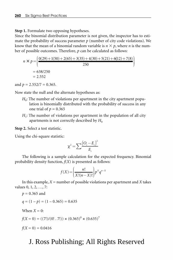
Step 1. Formulate two opposing hypotheses.Since the binomial distribution parameter is not given, the inspector has to esti-mate the probability of success parameter p (number of city code violations). Weknow that the mean of a binomial random variable is n � p, where n is the num-ber of possible outcomes. Therefore, p can be calculated as follows:
= 638/250= 2.552
and p = 2.552/7 = 0.365.
Now state the null and the alternate hypotheses as:
H0: The number of violations per apartment in the city apartment popu-lation is binomially distributed with the probability of success in anyone trial of p = 0.365
H1: The number of violations per apartment in the population of all cityapartments is not correctly described by H0
Step 2. Select a test statistic.
Using the chi-square statistic:
The following is a sample calculation for the expected frequency. Binomialprobability density function, f(X) is presented as follows:
In this example, X = number of possible violations per apartment and X takesvalues 0, 1, 2, …, 7:
p = 0.365 and
q = (1 – p) = (1 – 0.365) = 0.635
When X = 0:
f(X = 0) = ((7!)/(0! . 7!)) × (0.365)0 × (0.635)7
f(X = 0) = 0.0416
f Xn
X n Xp qX n X( )
!
!( )!=
−
⎛
⎝⎜⎜⎜
⎞
⎠⎟⎟⎟⎟
−
χ2
2
=−( )∑
O E
Ei i
i
n p( ) ( ) ( ) ( ) ( ) ( )
�� =+ + + + + +0 29 1 50 2 65 3 35 4 30 5 21 6(( ) ( )12 7 8
250
+⎛
⎝⎜⎜⎜
⎞
⎠⎟⎟⎟⎟
260 Six Sigma Best Practices
J. Ross Publishing; All Rights Reserved

The expected frequency (if H0 is true) when X = 0 is equal to 0.0416 × 250 = 10.4.
When X = 1:
f(X = 1) = ((7!)/(1! . 6!)) × (0.365)1 × (0.635)6
f(X = 1) = 0.1675
The expected frequency when X = 1 is equal to 0.1675 × 250 = 41.9.
Remaining calculations can be done as presented above.
Step 3. Derive the decision rule.First establish the expected frequencies for the various numbers of possible viola-tions per apartment, assuming H0 is true. Calculate the binomial probability value(or check in binomial table) for each possible violation (0, 1, 2, 3, 4, 5, 6, and 7)per apartment for given n = 8 and P = 0.365. Now calculate the expected fre-quency (Ei, i = 0, 1, 2, …, 7) for each possible apartment violation by multiplyingthe calculated probability by the total number of observations (250). Note: Keepthe expected frequency value of 5 or higher by combining adjacent classes asneeded.
Next establish the number of degrees of freedom (df):
df = number of classes (adjusted) – 1 – number of estimated parameters
Binomial distribution has only one parameter and the given desired signifi-cance level of α = 0.05 and the adjusted df. Find the χ2 value from the chi-squaretable. Compute the test statistic and then confront it with the decision rule. If thecalculated value (χ2
cal) is less than the table value (χ2table), accept the null (H0)
hypothesis; otherwise reject the null hypothesis.Next, perform a chi-square goodness-of-fit test using MINITAB software.
Since the population distribution is assumed to be binomial, the first activity is tocalculate the expected number of outcomes for the binomial case:
1. Enter the possible outcomes 0, 1, 2, 3, 4, 5, 6, and 7 in a work sheetunder Outcomes and enter observed frequency in the next column(C2) under Observed
2. Choose Calc > Probability Distribution > Binomial
3. In Number of trials, enter 7; in Probability of success, enter 0.365
4. Choose Input Column, then enter Outcomes; in Optional storage,enter Probs to name the storage column; click OK
5. Choose Calc > Calculator
6. In Store result in variable, enter Expected to name the storage column
7. In Expression, enter Probs*250; click OK
Analyze 261
J. Ross Publishing; All Rights Reserved

Next, calculate the χ2 statistics and P-value:
1. Choose Calc > Calculator
2. In Store result in variable, enter Chisquare to name the storage column
3. In Expression, enter SUM((Observed-Expected)**2/Expected); clickOK
4. Choose Calc > Probability Distribution > Chi-Square
5. Choose Cumulative probability and in Degrees of freedom, enter 4[The degrees of freedom value is equal to the number of (adjusted)classes minus one and minus one parameter (6 – 1 – 1 = 4).]
6. Choose Input column and enter Chisquare; in Optional storage,enter CumProb to name the storage column; click OK
7. Choose Calc > Calculator
8. In Store result in variable, enter Pvalue to name the storage column
9. In Expression, enter 1 – CumProb; click OK
The work sheet output is presented in Table 4.9B.
The P-value of 0.00 associated with the χ2 statistic of 372.923 indicates thebinomial probability model with p = 0.365 is probably not a good model for thisexperiment (test), i.e., the observed number of outcomes is not consistent withexpected number of outcomes using a binomial model. Therefore, reject the nullhypothesis.
Other examples of a goodness-of-fit test include:
262 Six Sigma Best Practices
Table 4.9B. Goodness of Fit Test Output
Chi- Cumulative P-Outcome Observed Probability Expected Square Probability Value
0 29 0.041631 10.4077 372.923 1 0
1 50 0.167505 41.8768
2 65 0.288851 72.2127
3 35 0.276721 69.1802
4 30 0.159060 39.7650
5 21 0.054857 13.7142
6 12 0.010511 2.6277 16.5577
7 8 0.000863 0.2158 }
J. Ross Publishing; All Rights Reserved

• Normally Distributed Population—A financial analyst would like todetermine if the daily volume of New York Stock Exchange is still nor-mally distributed with a mean of 50 million trades and a standarddeviation of 5 million trades.
• Uniformly Distributed Population—A business management team ofa house cleaning service wants to know if service requests are spreadevenly over the six business days of a business week. Accordingly, thisinformation will be used to set work schedules for employees.
Therefore, chi-square tests are used for:
• Goodness of Fit—To test if the sample data have the same distribu-tion as expected
• Test of Independence—To test if the samples are from the same dis-tribution
Limitations when using the chi-square test include:
• Use discrete data. Use no ranking or variable data.
• Observations must be independent.
• The chi-square test works best with five or more observations in eachcell. Cells may be combined (to make a larger range) to pool observa-tions.
Exercise 4.3: Determining the Distribution of Passengers Arriving at aLuggage Checkout
An airline manager wants to determine if the Poisson distribution can describethe number of hourly passenger arrivals at the luggage checkout area. A test at the1% level of significance is to be conducted. A simple random sample over 48hours has been collected (Table 4.9C).
Based on prior experience of the airline manager, the passenger mean arrivalrate is four passengers per hour, assuming the Poisson probability distribution.Perform a detailed analysis to verify the summary information in Table 4.9D.
Based on the summary information in Table 4.9D, the P-value of 0.640743associated with the χ2 statistic of 6.05793 indicates that the Poisson probabilitymodel with λ = 4 (mean passenger arrival rate per hour) is probably a good modelfor this experiment, i.e., the observed number of outcomes is consistent withexpected number of outcomes using a Poisson model. Give an opinion of thesecomments.
Next is a discussion of ANOVA (the analysis of variance), which takes thistype of analysis one step further.
Analyze 263
J. Ross Publishing; All Rights Reserved

4.4 ANALYSIS OF VARIANCE (ANOVA)
Reengineering and/or redesigning processes are a natural part of the responsibil-ities of any Six Sigma team. As discussed in the previous section, the normal prob-ability distribution (for large samples) and the Student’s t-distribution (for smallsamples) are ideally suited to assist in performing any desired hypothesis testabout the comparative magnitudes of two population means. This section willtake this type of analysis a step further. The means of more than two quantitativepopulations will be compared, leading to the conclusion that such extended com-parisons are not performed well using the earlier procedures.
Consider two situations. In one, a production manager wants to test if theaverage daily throughput differs among six possible production methods. In theother, a store manager wants to know if average sales vary among five alternatives:newspaper ads, TV ads, window displays, type of packaging, and price levels.
Tempting as it may be, it is unwise to string together the results of several two-sample tests. Therefore, an analysis of variance (ANOVA) table will assist in deter-mining the effect of multiple input variables on a response.
Analysis of variance (commonly known as ANOVA) is a statistical techniqueespecially designed to test if the means of more than two quantitative populationsare equal. If the equality of only two means is tested, then the test will yield thesame results as the normal distribution or the t-distribution discussed in the pre-vious section. The ANOVA technique involves taking an independent simple ran-dom sample from each of several populations of interest and then analyzing thedata. Similar to the t-test, the ANOVA test also assumes that the sampled popula-
264 Six Sigma Best Practices
Table 4.9C. Collected Sample Data from LuggageCheckout Area
Number of Passenger Arrivals Observed per Hour to Luggage Passenger
Checkout Area Frequency
0 01 12 53 84 135 96 77 3
8 or more 2
J. Ross Publishing; All Rights Reserved
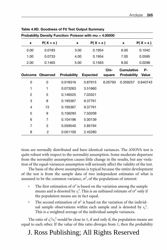
tions are normally distributed and have identical variances. The ANOVA test isquite robust with respect to the normality assumption. Some moderate departurefrom the normality assumption causes little change in the results, but any viola-tion of the equal-variances assumption will seriously affect the validity of the test.
The basis of the above assumptions is typical because the entire developmentof the test is from the sample data of two independent estimates of what isassumed to be the common variance, σ2, of the populations of interest:
• The first estimation of σ2 is based on the variation among the samplemeans and is denoted by st
2. This is an unbiased estimate of σ2 only ifthe population means are in fact equal.
• The second estimation of σ2 is based on the variation of the individ-ual sample observations within each sample and is denoted by se
2.This is a weighted average of the individual sample variances.
The ratio of st2/se
2 would be close to 1, if and only if, the population means areequal to each other. If the value of this ratio diverges from 1, then the probability
Analyze 265
Table 4.9D. Goodness of Fit Test Output Summary
Probability Density Function: Poisson with mu = 4.00000
x P( X = x ) x P( X = x ) x P( X = x )
0.00 0.0183 3.00 0.1954 6.00 0.1042
1.00 0.0733 4.00 0.1954 7.00 0.0595
2.00 0.1465 5.00 0.1563 8.00 0.0298
Chi- Cumulative P-Outcome Observed Probability Expected square Probability Value
0 0 0.018316 0.87915 6.05793 0.359257 0.640743
1 1 0.073263 3.51660
2 5 0.146525 7.03321
3 8 0.195367 9.37761
4 13 0.195367 9.37761
5 9 0.156293 7.50209
6 7 0.104196 5.00139
7 3 0.059540 2.85794
8 2 0.051100 2.45280
J. Ross Publishing; All Rights Reserved

would be greater that the population means are not equal to each other. In prin-ciple, this ratio of squares can take any value between zero and positive infinity.Therefore, ANOVA helps test hypotheses about the equality of means.
Two types of problem analysis are commonly used:
• One-Factor ANOVA or One-Way ANOVA—A completely randomizeddesign uses randomization as a control device. This design creates onetreatment group for each treatment and assigns each experimentalunit to one of these groups by a random process. In the end, only onefactor (the treatment) is considered as possibly affecting the variableof interest. Analysis of this type of problem is referred to as one-fac-tor ANOVA or one-way ANOVA. (See Chapter 5, Improve; Section 5.3,Introduction to Design of Experiments, for further discussion of thisconcept.)
• Two-Factor ANOVA or Two-Way ANOVA—A randomized block designuses blocking as an additional control device. It divides the availableexperimental units into specifically different, but internally homoge-neous blocks and then randomly matches each treatment with one ormore units within any given block. This treatment is believed to havean effect within any one block only, but also possible is observingpotential differences for any given treatment among blocks. An analy-sis of this type of problem is referred to as two-factor ANOVA or two-way ANOVA. (Any statistics textbook may be consulted for additionaldetails.)
One-Way ANOVAExamples can facilitate understanding the concept of one-way ANOVA.
Example 4.11: Analyzing Rice Yield
In a 1-year study, 20 experimental plots in which rice was grown were observed.Then 5 plots were randomly selected for each group, and all 20 plots were dividedinto 4 groups. Four different types of fertilizer (1, 2, 3, and 4) were applied, one ineach group of five plots. Determine whether four different types of fertilizer areequally effective at a 5% significance level or if they are not. A completely ran-domized plot design was developed. The rice yield data were measured in pounds(Table 4.10A). To analyze the data, formulate the opposing hypotheses:
H0: The mean pounds of rice yield for all 5 plots in which fertilizer type 1was applied are the same as those for the application of fertilizers 2, 3,and 4, i.e., μ1 = μ2 = μ3 = μ4
266 Six Sigma Best Practices
J. Ross Publishing; All Rights Reserved

H1: The mean rice yield from at least one of plot group is different fromthe others, i.e., at least one of the equalities does not hold
The body of the table has four rows (r = 4) and five columns (c = 5) in whichrice yield data have been stored. Study the yield variation in the sample data. Thisvariation has two components:
• Variation among rows: Explained by fertilizer treatments
• Variation within rows: Due to error
Variation among rows: explained by fertilizer treatments. The variationamong the r = 4 sample means ( ⎯X1, ⎯X2, ⎯X3, and ⎯X4) that summarize the data asso-ciated with each of the fertilizer treatments is known as explained variation ortreatment variation. This variation is not attributable to chance, but to inherentdifferences among the treatment populations. (Remember from an earlier discus-sion that the measurement of this variation constitutes the first estimate, st
2, of thepopulation variance, σ2.) This estimate is based on several considerations:
Given: The assumed normality of the sampled populations, the sampling distri-bution of each sample mean, ⎯Xi, where, i = 1, 2, 3, and 4 represents treat-ments, will be normally distributed:
Let:
σ2⎯Xi
= Variance among treatment population, i = 1, 2, 3, 4
σ2 = Population variance
then,
Analyze 267
Table 4.10A. Collected Sample Data of Rice Yield from Plots
Treatment, i Plot, j(Type of Fertilizer Sample
Applied) 1 2 3 4 5 Total Mean
1 19 15 22 17 19 92 ⎯X1 = 18.4
2 20 25 21 19 22 107 ⎯X2 = 21.4
3 18 12 17 16 16 79 ⎯X3 = 15.8
4 20 17 16 15 15 83 ⎯X4 = 16.6
Grand Mean: ⎯X = 18.05
J. Ross Publishing; All Rights Reserved

Assume: Equality of population variances, i.e.: σ21 = σ2
2 = σ23 = σ2
4 and equalsample sizes (n1 = n2 = n3 = n4)
Then the value of σ2⎯Xi
is the same for each i, and sample size in each treatment isequal to column (c).
Therefore:
σ2 = nσ2⎯X = cσ2
⎯X and =X = Grand mean
The variance of the sample distribution of ⎯X can be calculated as:
From previous equations,
and
= Treatments sum of squares (or TSS)
For the sample data,
TSS = 5[(18.4 – 18.05)2 + (21.4 – 18.05)2 + (15.8 – 18.05)2
+ (16.6 – 18.05)2]= 92.05
and the degrees of freedom (df) associated with the estimation of σ2 with the helpof the variation among sample means. Therefore,
df = r – 1 = 4 – 1 = 3 (in the example)
σ2 can be estimated from the sample data, as follows:
σ 22
1≅
−−
⎛
⎝
⎜⎜⎜⎜⎜
⎞
⎠
⎟⎟⎟⎟⎟∑c X X
ri( )
( )
c X Xi( )∑ − 2
σ σ2 2
2
1= ≅
−( )−( )
⎛
⎝
⎜⎜⎜⎜⎜⎜⎜
⎞
⎠
⎟⎟⎟⎟⎟⎟⎟⎟
∑c
c X X
rX
i
σ X Xis
X X
r2 2
2
1≅ =
−−
∑( )
( )
σσ
Xi
ii n
22
=⎛
⎝⎜⎜⎜⎜
⎞
⎠⎟⎟⎟⎟⎟
268 Six Sigma Best Practices
J. Ross Publishing; All Rights Reserved

This is known as treatments mean square (TMS) and also as explained varianceand is identical to the population variance estimate symbolized by st
2 above.In the example,
TMS = st2 = TSS/(r – 1)
= 92.05/(4 – 1) = 30.68
Variation within rows: due to error. The variation of the sample data withineach of the r = 4 rows (or samples) about the respective sample mean is known asunexplained variation or residual variation or simply as (experimental or sam-pling) error and it is attributed to chance. As noted above, the measurement of thisvariation constitutes a second estimate, se
2, of the population variance, σ2, and thisestimate is based on the considerations that from each of the treatment samples(i), a sample variance can be derived as follows:
where:
Xij = Sample observations in row i and column j
⎯Xi = Mean of sample i, where i = 1, 2, 3, and 4
ni = number of observations in sample i
To obtain a single estimate of σ2, take the weighted average of the i samplevariances,
= Error mean square (EMS) or explained variance
= se2
and
ΣΣ(Xij – ⎯Xi)2 = Error sum of squares (ESS)
(c – 1) × r = df
Calculations for the ESS are presented in Table 4.10B. Based on the Table4.10B data:
σ 2
2
1≅
−
−∑∑ ( )
( )
X X
c rij i
sX X
ni
ij i
i
2
2
1=
−
−∑( )
Analyze 269
J. Ross Publishing; All Rights Reserved

ESS = 27.2 + 21.2 + 20.8 + 17.2 = 86.4
df = (c –1) × r = (5 – 1) × 4 = 16
σ2 � EMS = se2
For the example:
EMS = 86.4/16 = 5.4
The ANOVA TableAn ANOVA table shows for each source of variation, the sum of squares (SS), thedegrees of freedom (df), and the ratio of the sum of squares to the df. The ratioof the sum of squares is called the mean square and it is the desired estimate of thepopulation variance. The last row of the table is called the Total Sum of Squares orTotal SS, which can be calculated independently by summing the squared devia-tions of each individual sample observation from the mean of all observations(grand mean).
In a one-way ANOVA table,
Total SS = TSS + ESS and
Total df = (r – 1) + (c – 1)r = rc – 1
A one-way ANOVA table for the sample data is presented in Table 4.10C.
The F DistributionThe ratio st
2/se2 is equal to TMS/EMS and would be close to 1 whenever the null
hypothesis of equal population means was true. This ratio is used as the ANOVAtest statistic and is denoted by F. The probability distribution of F helps in decid-ing if any given divergence of F from 1 is significant enough to warrant the rejec-tion of the null hypothesis of equal population means. In contrast to the t and χ2
270 Six Sigma Best Practices
Table 4.10B. Error Sum of Squares Data
ObservationTreatment
i 1 2 3 4 5 Total
(X1j – ⎯X1)2 (19 – 18.4)2 = 0.36 11.56 12.96 1.96 0.36 27.2
(X2j – ⎯X2)2 (20 – 21.4)2 = 1.96 12.96 0.16 5.76 0.36 21.2
(X3j – ⎯X3)2 (18 – 15.8)2 = 4.84 14.44 1.44 0.04 0.04 20.8
(X4j – ⎯X4)2 (20 – 16.6)2 = 11.56 0.16 0.36 2.56 2.56 17.2
J. Ross Publishing; All Rights Reserved
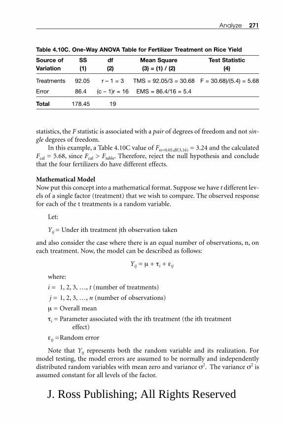
statistics, the F statistic is associated with a pair of degrees of freedom and not sin-gle degrees of freedom.
In this example, a Table 4.10C value of Fα=0.05,df(3,16) = 3.24 and the calculatedFcal = 5.68, since Fcal > Ftable. Therefore, reject the null hypothesis and concludethat the four fertilizers do have different effects.
Mathematical ModelNow put this concept into a mathematical format. Suppose we have t different lev-els of a single factor (treatment) that we wish to compare. The observed responsefor each of the t treatments is a random variable.
Let:
Yij = Under ith treatment jth observation taken
and also consider the case where there is an equal number of observations, n, oneach treatment. Now, the model can be described as follows:
Yij = μ + τi + εij
where:
i = 1, 2, 3, …, t (number of treatments)
j = 1, 2, 3, …, n (number of observations)
μ = Overall mean
τi = Parameter associated with the ith treatment (the ith treatment effect)
εij =Random error
Note that Yij represents both the random variable and its realization. Formodel testing, the model errors are assumed to be normally and independentlydistributed random variables with mean zero and variance σ2. The variance σ2 isassumed constant for all levels of the factor.
Analyze 271
Table 4.10C. One-Way ANOVA Table for Fertilizer Treatment on Rice Yield
Source of SS df Mean Square Test StatisticVariation (1) (2) (3) = (1) / (2) (4)
Treatments 92.05 r – 1 = 3 TMS = 92.05/3 = 30.68 F = 30.68)/(5.4) = 5.68
Error 86.4 (c – 1)r = 16 EMS = 86.4/16 = 5.4
Total 178.45 19
J. Ross Publishing; All Rights Reserved

Mathematical Hypotheses:
H0: τ’s = 0 (Null hypothesis assumes the treatment term is zero)
H1: τi ≠ 0 (For at least one i)
Conventional Hypotheses:
H0: μ1 = μ2 = … = μi=t
H1: At least one μi is different
ANOVA Steps:
Step 1. State the problem.
Step 2. Model assumptions:
• Treatment response means are independent and normally distributed:
– The experiment run must be randomized.
– The sample size must be good.
– Run a normality test on the collected data. When using MINITABsoftware: Stat > Basic Stats > Normality Test
• Homogeneity test of population variances should be equal across alllevels of factors:
Therefore, for σ:
H0: σpopulation1 = σpopulation2 = …; and
H1: At least two are different
Step 3. State the hypotheses.
Step 4. Develop an ANOVA table.
Step 5. Check that the errors of the model are independent and normally distrib-uted. Ways to check include:
• Run a normality check on error terms.
• Plot residuals against fitted values.
• Randomize runs during the experiment.
• Ensure adequate sample size.
• Plot a histogram of error terms.
Step 6. Interpret the P-value and/or the F-statistic for the factor or treatmenteffect.
272 Six Sigma Best Practices
J. Ross Publishing; All Rights Reserved

For example:
At α = 0.05, P-value < 0.05, then reject H0.
Otherwise, assume the null hypothesis is true. The test performer must evaluateP-value before making any decision.
In the case of F-statistic:If Fcalculated < Ftable, then accept the H0
Otherwise, assume the alternate hypothesis is true.
Step 7. Calculate epsilon squared for the treatment and error terms.
ε2treatment = (Treatment SS)/(Total SS)
ε2error = (Error SS)/(total SS)
Note: The epsilon-square (ε2) statistic is not universally acceptable. This sta-tistic is a guideline of the significance of treatment effect. It is also a measure ofvariation of the output in relation to input.
Step 8. Translate the technical output from the test into simple language.
Now, work with the same example (Example 4.11), using MINITAB softwareand following the ANOVA steps.
Step 1. State the problem:
• A scientist would like to know whether all fertilizer treatments couldaffect rice yield equally or if they will not.
• Plot the data. Plotting the collected data is important. Two data plots(dot plots and box plots) have been developed using the collectedsample data (Figures 4.8A and 4.8B, respectively). These plots presentpictorial views of the sample data.
Step 2. Model assumptions:
• Run the normal probability plot to check that response means areindependent and normally distributed (Figure 4.8C).
– Generally run randomize runs during the experiment and data col-lection.
– Ensure that sample size is adequate (sample >30). Sample size inthis example = 20.
– Run a normality test on the data:
Analyze 273
J. Ross Publishing; All Rights Reserved

• Use MINITAB software: Stat > Basic Stats > Normality Test.
• The Anderson-Darling normality test is used here.
274 Six Sigma Best Practices
t4t3t2t1
25
20
15
Fertilizer
Res
pons
e
*Group means are indicated by lines
Figure 4.8A. Dot Plot of Fertilizer Treatment on Rice Yield*
t4t3t2t1
25
20
15
Fertilizer
Res
pons
e
*Means are indicated by solid circles.
Figure 4.8B. Box Plot of Fertilizer Treatment on Rice Yield*
J. Ross Publishing; All Rights Reserved

• Perform homogeneity of variance analysis to check that the popula-tion variances are equal across all levels of treatment (factor). Theassumption of equal variance generally holds if the number of obser-vations for each treatment is the same. MINITAB data are presentedin Table 4.10D and Figure 4.8D.
For s:
H0: spopulation1 = spopulation2 = spopulation3 = spopulation4
H1: At least two are different
Step 3. State the hypotheses:
H0: μferti1 = μferti2 = μferti3 = μferti4
H1: At least two fertilizer treatments are different
or
H0: τ’s = 0 (null hypothesis assumes the treatment term is zero)
H1: τ’s ≠ 0
Analyze 275
252015
.999
.99
.95
.80
.50
.20
.05
.01
.001
Pro
babi
lity
Response
Average: 18.05StDev: 3.06894N: 20
Anderson-Darling Normality TestA-Squared: 0.278P-Value: 0.613
Figure 4.8C. Normality Test using Anderson-Darling Test
J. Ross Publishing; All Rights Reserved

• Null hypothesis—Average rice yield from each plot is the same or fer-tilizer treatments will not have a significantly different yield fromplots.
• Alternate hypothesis—At least one fertilizer treatment will affect aver-age rice yield.
Step 4. Develop an ANOVA table. The developed ANOVA table is presented inTable 4.10E.
• Use MINITAB software: Stat > ANOVA > Oneway …
Note: Store residuals and fits for later use.
276 Six Sigma Best Practices
Table 4.10D. Equal Variance Test Data
Response: ResponseFactor: FertilizerConfidence Level: 95.0000
Lower Sigma Upper N Factor Levels
1.37662 2.60768 10.8186 5 t11.21534 2.30217 9.5512 5 t21.20382 2.28035 9.4606 5 t31.09470 2.07364 8.6030 5 t4
Note: Bonferroni confidence intervals for standard deviations.
1050
t4
t3
t2
t1
95% Confidence Intervals for Sigmas Factor Levels
Bartlett's TestTest Statistic: 0.195P-Value : 0.978
Levene's TestTest Statistic: 0.069P-Value : 0.976
Figure 4.8D. Homogeneity of Variance Test for Rice Yield
J. Ross Publishing; All Rights Reserved

Step 5. Check that errors of the model are independent and normally distributed.Three graphs have been plotted (Figures 4.8E, 4.8F, and 4.8G). The graph plottedin Figure 4.8E checks the residual normality. The histogram plotted in Figure 4.8Fshould appear as a bell curve, but in this example the bell curve shape can beignored because the sample is small (<30). Figure 4.8G shows that the residualsshould be random about 0 (zero) without trends. The graph in Figure 4.8G inves-tigates if the mathematical model fits equally for low to high values of the fit.
Step 6. Interpret the P-value and/or the F-statistic for the factor or treatmenteffect. For example:
At α = 0.05, P-value< 0.05, reject H0
Otherwise, assume the null hypothesis is true.
An analysis of variance for treatment response is presented in Table 4.10F. Whengroup sizes are equal, σ2
pooled = (σ12 + σ2
2 + σ32 + σ4
2 )/4; this value in Table 4.10Fis 5.40. The table value of F (Fa=0.05,df(3,16)) is 3.24; the calculated value from Table4.10F is 5.71.
Since the Fcalculated > Ftable, therefore, the null hypothesis is rejected.
Another check for the hypothesis test is the P test. Since α = 0.05 and the cal-culated value of P is 0.007, at least one group mean is different. Therefore, again
Analyze 277
Table 4.10E. One-Way ANOVA Table—Rice Yield vs. Fertilizer Treatment
Analysis of Variance for Response
Source df SS MS F P
Fertilizer 3 92.55 30.85 5.71 0.007Error 16 86.40 5.40Total 19 178.95
Individual 95% CIs for MeanBased on Pooled SD
Level N Mean SD -----+---------+---------+---------+-
t1 5 18.400 2.608 (------*-------) t2 5 21.400 2.302 (------*-------) t3 5 15.800 2.280 (-------*------) t4 5 16.600 2.074 (------*-------)
-----+---------+---------+---------+-
Pooled SD = 2.324 15.0 18.0 21.0 24.0
J. Ross Publishing; All Rights Reserved

278 Six Sigma Best Practices
–4 –3 –2 –1 0 1 2 3 4
Nor
mal
Sco
re
Residual
*Response is Response
–2
–1
0
1
2
–4 –3 –2 –1 0 1 2 3 4
0
1
2
3
4
Residual
Fre
quen
cy
*Response is Response.
Figure 4.8E. Normal Probability Plot of the Residuals*
Figure 4.8F. Histogram of Residuals*
J. Ross Publishing; All Rights Reserved

the null hypothesis that all the group means are equal is rejected. At least one fer-tilizer treatment mean is different.
Step 7. Calculate epsilon squared for the treatment and error terms:
ε2treatment = (Treatment SS)/(Total SS)
ε2treatment = (92.55)/(178.95) = 0.52
Therefore, 52% of the variation in rice yield can be explained by fertilizer treat-ment.
Step 8. Translate the technical output from the test into simple language, e.g.: “Wehave found that fertilizer treatment does affect rice yield. Fertilizer treatment twoprovides the highest yield.”
Exercise 4.4: Comparing Average Cost of Market Basket Goods inFour Cities
A nonprofit organization wants to test, at the 1% level of significance, if the aver-age cost of a given market basket of goods is the same in four cities (Boston,Chicago, Dallas, and Los Angeles). A random sample of eight stores in each of thecities has provided the data (see Table 4.11 for average cost of a given market
Analyze 279
15.5 16.5 17.5 18.5 19.5 20.5 21.5
*Response is Response.
Fitted Value
–4
–3
–2
–1
0
1
2
3
4R
esid
ual
Figure 4.8G. Residuals vs. Fitted Values*
J. Ross Publishing; All Rights Reserved
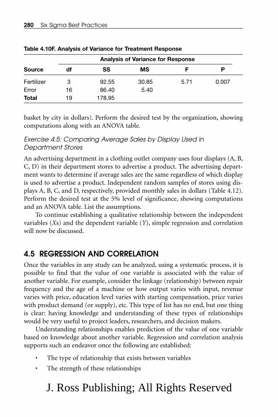
basket by city in dollars). Perform the desired test by the organization, showingcomputations along with an ANOVA table.
Exercise 4.5: Comparing Average Sales by Display Used inDepartment Stores
An advertising department in a clothing outlet company uses four displays (A, B,C, D) in their department stores to advertise a product. The advertising depart-ment wants to determine if average sales are the same regardless of which displayis used to advertise a product. Independent random samples of stores using dis-plays A, B, C, and D, respectively, provided monthly sales in dollars (Table 4.12).Perform the desired test at the 5% level of significance, showing computationsand an ANOVA table. List the assumptions.
To continue establishing a qualitative relationship between the independentvariables (Xs) and the dependent variable (Y), simple regression and correlationwill now be discussed.
4.5 REGRESSION AND CORRELATIONOnce the variables in any study can be analyzed, using a systematic process, it ispossible to find that the value of one variable is associated with the value ofanother variable. For example, consider the linkage (relationship) between repairfrequency and the age of a machine or how output varies with input, revenuevaries with price, education level varies with starting compensation, price varieswith product demand (or supply), etc. This type of list has no end, but one thingis clear: having knowledge and understanding of these types of relationshipswould be very useful to project leaders, researchers, and decision makers.
Understanding relationships enables prediction of the value of one variablebased on knowledge about another variable. Regression and correlation analysissupports such an endeavor once the following are established:
• The type of relationship that exists between variables
• The strength of these relationships
280 Six Sigma Best Practices
Table 4.10F. Analysis of Variance for Treatment Response
Analysis of Variance for Response
Source df SS MS F P
Fertilizer 3 92.55 30.85 5.71 0.007Error 16 86.40 5.40Total 19 178.95
J. Ross Publishing; All Rights Reserved
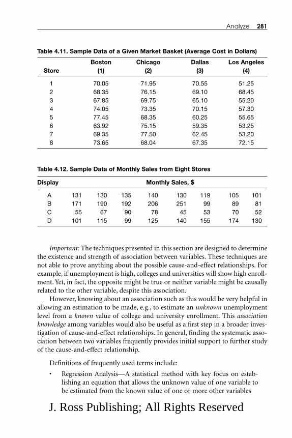
Important: The techniques presented in this section are designed to determinethe existence and strength of association between variables. These techniques arenot able to prove anything about the possible cause-and-effect relationships. Forexample, if unemployment is high, colleges and universities will show high enroll-ment. Yet, in fact, the opposite might be true or neither variable might be causallyrelated to the other variable, despite this association.
However, knowing about an association such as this would be very helpful inallowing an estimation to be made, e.g., to estimate an unknown unemploymentlevel from a known value of college and university enrollment. This associationknowledge among variables would also be useful as a first step in a broader inves-tigation of cause-and-effect relationships. In general, finding the systematic asso-ciation between two variables frequently provides initial support to further studyof the cause-and-effect relationship.
Definitions of frequently used terms include:
• Regression Analysis—A statistical method with key focus on estab-lishing an equation that allows the unknown value of one variable tobe estimated from the known value of one or more other variables
Analyze 281
Table 4.11. Sample Data of a Given Market Basket (Average Cost in Dollars)
Boston Chicago Dallas Los AngelesStore (1) (2) (3) (4)
1 70.05 71.95 70.55 51.252 68.35 76.15 69.10 68.453 67.85 69.75 65.10 55.204 74.05 73.35 70.15 57.305 77.45 68.35 60.25 55.656 63.92 75.15 59.35 53.257 69.35 77.50 62.45 53.208 73.65 68.04 67.35 72.15
Table 4.12. Sample Data of Monthly Sales from Eight Stores
Display Monthly Sales, $
A 131 130 135 140 130 119 105 101B 171 190 192 206 251 99 89 81C 55 67 90 78 45 53 70 52D 101 115 99 125 140 155 174 130
J. Ross Publishing; All Rights Reserved

• Regression Equation—A prediction equation that could be linear orcurvilinear, which allows the unknown value of one variable to beestimated from the known value of one or more other variables
• Regression Line—In regression analysis, a line that summarizes therelationship between an independent variable, X, and a dependentvariable, Y, while also minimizing the errors made
• Coefficient of Determination: r2—Measures how well the estimatedregression line fits the sample data or the amount of variationexplained by the regression equation
• Coefficient of Correlation: √r2 = r—The square root of the samplecoefficient of determination, which is a common alternative index ofthe degree of association between two quantitative variables
• Coefficient of Determination (Adjusted): r2(Adj)—The r2(Adj) fordegrees of freedom (If a variable is added to an equation, r2 willalmost always get larger, even if the added variable is of no real value.)
Simple regression analysis and simple correlation analysis will now be dis-cussed:
• Simple Regression Analysis—A method in which a single variable isused to estimate the value of an unknown variable
• Simple Correlation Analysis—A statistical method in which a keyfocus is the establishment of an index that provides, in a single num-ber, an instant measure of the strength of association between twovariables (Depending on the value of this measure (0 to 1), howclosely two variables move together can be determined and, thereby,with what degree of confidence one variable can be estimated with thehelp of the other.)
4.5.1 Simple Regression AnalysisIn regression analysis, there are two types of variables, X and Y. The value of avariable assumed known is symbolized by X and is referred to as the independentvariable or predictor variable. In contrast, the value of the variable assumedunknown is symbolized by Y and is referred to as the dependent variable or pre-dicted variable.
The relationship between these X and Y variables can be deterministic or sto-chastic. If the relationship is precise, exact, or deterministic, the value of Y isuniquely determined whenever the value of X is specified. In contrast, the rela-tionship can be an imprecise, inexact, or stochastic, in such a way that many pos-sible values of Y can be associated with any one value of X. Only the deterministicmodel will be discussed in this section.
282 Six Sigma Best Practices
J. Ross Publishing; All Rights Reserved

Figure 4.9 contains panels of the alternative relationships between X and Y.Each dot in the graphs represents a hypothetical pair of observations about anindependent variable X and a dependent variable Y. The lines summarize thenature of their relationship.
Panel (1) is described by the equation Y = c + mX. In this particular example,X and Y are variables, while c is the vertical intercept and m is the slope of thestraight line. Both c and m are defined as constants. The slope could be positive
Analyze 283
.
.. .
. ..
..
. ..
.
.
.
.
....
.
.. …
..
. ...
..
..
..
..
.
.
.
..
..
.
...
..
.. ..
.
.. . .. ... ..
. .. .. . ...
..
...
. ....
.
...
. ..
. .
.
.
.
..
.
.
.
.
.
. ..
.
.
.. .
.
.
.
. .
.
....
.. .
.
....
.
...
. .. .. .
. .. ...
.... ... .. . .. .
.....
.
.
(1) (2)
(3) (4)
∧Yx = c + mx
∧Yx = c – mx
X X
Y Y
X X
Y Y
∧Yx = c + mx – x2
∧Yx = c + mx + ax2
.
.... .
..
.. .
.
.
.
.
. .... .. . .. .
.
. ... .. .. .
.
. ..
. .
. .
. .. ... . .
.
. .
.
. .
.
.
... .
..
.
.
. .
..
..
.. .
..
. ..
.
.
.
.
.
.
.
..
. ..
.
.
.
.
.
..
.
.
. .
.
.
.
.
. .
..
.
.
.. .
.
.
.
..
.
...
..
.
..
.
.
.
.
.
.. ..
.. . ...
.
... .
. ..
.... . .
. ...... .. . .
.
. ..
.
..
.
.
.
..
...
. .
(5) (6)
(7) (8)
X X
Y Y
X X
Y Y
∧Y = mx
∧Yx = c + mx – ax2 + x3
∧Y = a e-bx
∧Yx = c + mlog(1 + x)
Figure 4.9. Relationships between X and Y
J. Ross Publishing; All Rights Reserved

or negative. For example, Panel (2) presents a straight regression relationship, butwith a negative slope. In Panel (1), as the value of the dependent variable Yincreases with the larger values of the independent variable X, there is said to bea direct relationship. The slope of this regression line is positive and is representedby m. If instead, as in Panel (2), the value of the dependent variable Y decreaseswith the larger values of the independent variable X, there is said to be an inverserelationship and the value of m is negative.
Panels (1) and (2) present a linear relationship and Panels (3) through (8)present curvilinear relationships. In addition, the relationship in Panels (1), (5),and (8) could be defined as direct; or it could be inverse, as presented in Panels (2)and (6); or it could be a combination of direct and inverse as presented in Panels(3), (4), and (7). Of course, the values of the constants (a, c, and m) do differ fromone equation to the next.
Essential: Carefully check the following elements when plotting collecteddata:
• Properly Identify the X and the Y Variables—Analyze the variablescorrectly for potential cause and effect. The process (independent)variable, as the predictor, is on the X axis and the output (dependent)or process performance variable, as the response, is on the Y axis.Important: When plotting data, a common mistake is mixing up the Xand Y variables.
• Properly Scale a Scatter Diagram—To have a proper interpretation ofdata, it is important to use, to the fullest possible extent, both the Xand Y axes to cover all the collected data. Improper scaling of any axiscan result in an obscured pattern. Divide the space on each axis so thatdata plotting and data reading are facilitated.
• Pair Data Correctly—The X and Y variables must be paired beforeplotting, i.e., there must be a logical correspondence between the datato appropriately study the correlation.
Finding the Regression Line—The Method of Least SquaresFitting the data to a line in a scatter diagram is known as the method of leastsquares (also least squares method), a commonly used approach. The line is devel-oped so that the sum of the squares of the vertical deviations between the line andthe individual data plots is minimized. These vertical deviations represent theerrors associated with using the regression line to predict Y with the help of X.Figure 4.10 shows the nature of the squares and the sum of these squares is beingminimized.
284 Six Sigma Best Practices
J. Ross Publishing; All Rights Reserved

A regression line from the sample data calculated by the least squares methodis known as the simple regression line or estimated regression line. The value ofparameters c and m in its equation:
are referred to as the estimated regression coefficients, and their values can be esti-mated as follows:
where:
m = Slope of the estimated regression line
c = Intercept of the estimated regression line
Xi = Observed values of the independent variable
Yi = Associated observed values of the dependent variable
i = 1, 2, 3, …, n number of observations
as presented in Example 4.12.
cY
nm
X
ni i=
⎛
⎝⎜⎜⎜⎜
⎞
⎠⎟⎟⎟⎟⎟−
⎛
⎝⎜⎜⎜⎜
⎞
⎠⎟⎟⎟⎟⎟
∑ ∑
m
X YX Y
n
X nX
n
i ii i
ii
=
−⎛
⎝⎜⎜⎜⎜
⎞
⎠⎟⎟⎟⎟⎟
−⎛
⎝⎜⎜⎜⎜
∑∑∑
∑2⎞⎞
⎠⎟⎟⎟⎟⎟∑
2
Y c mXX = +
Analyze 285
.
.
..
.
X
Y
0
.
.
.
Figure 4.10. The Method of Least Squares
J. Ross Publishing; All Rights Reserved

Example 4.12: Using the Least Squares Method to Develop aRegression Equation
Twenty sample data points and in-process information are presented in Table4.13A. Based on the available information:
⎯X = ΣXi /n= 240/20= 12
⎯Y = SYi /n= 475/20= 23.75
= (6392 – ((240 × 475)/20)) / (3262 – 20(240/20)2)= 692/382
m = 1.812
= (475 / 20) –1.812 (12)c = 2.006
Therefore, the regression equation is:
Yi = 2.006 + 1.812 Xi
If the developed regression equation is utilized, the estimated values for thedependent variable (Y) can be obtained. The three selected points are whereX = 8, 12, and 15 and the calculated Y = 16.5, 23.75, and 29.19, respectively. Nowthe collected data values can be compared with the estimated values in Table4.13B.
Example 4.13: Using MINITAB Software—The Estimated vs. the TrueRegression Line
Imagine a scatter diagram for the population, not just a sample. For each andevery value of X, there would be a value of Y, but there would be a multitude of
cY
nm
X
ni i=
⎛
⎝⎜⎜⎜⎜
⎞
⎠⎟⎟⎟⎟⎟
−⎛
⎝⎜⎜⎜⎜
⎞
⎠⎟⎟⎟⎟⎟
∑ ∑
m
X YX Y
n
X nX
n
i ii i
ii
=
−⎛
⎝⎜⎜⎜⎜
⎞
⎠⎟⎟⎟⎟⎟
−⎛
⎝⎜⎜
∑∑∑
∑2
⎜⎜⎜
⎞
⎠⎟⎟⎟⎟⎟∑
2
286 Six Sigma Best Practices
J. Ross Publishing; All Rights Reserved

Analyze 287
Table 4.13A. Utilizing the Least Squares Method to Establish the Regression Line
Count, i Xi Yi XiYi Xi2
1 2 5 10 42 4 9 36 163 8 25 200 644 8 9 72 645 8 20 160 64
6 12 20 240 1447 13 25 325 1698 14 30 420 1969 14 25 350 196
10 15 30 450 225
11 10 25 250 10012 12 25 300 14413 12 26 312 14414 12 22 264 14415 11 18 198 121
16 15 26 390 22517 21 45 945 44118 16 35 560 25619 16 25 400 25620 17 30 510 289
Table 4.13B. Projected and Actual Values of Dependent Variable in Relation toIndependent Variable
Dependent Variable Y
Independent Actual Collected Estimated ValueVariable Value Through Through the
X Sample Regression Equation
8 25, 9, 20 16.5
12 20, 25, 26, 22 23.75
15 30, 26 29.19
J. Ross Publishing; All Rights Reserved
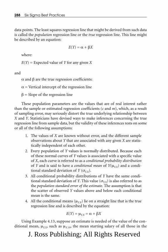
data points. The least squares regression line that might be derived from such datais called the population regression line or the true regression line. This line mightbe described by an equation:
E(Y) = α + βX
where:
E(Y) = Expected value of Y for any given X
and
α and β are the true regression coefficients:
α = Vertical intercept of the regression line
β = Slope of the regression line
These population parameters are the values that are of real interest ratherthan the sample or estimated regression coefficients (c and m), which, as a resultof sampling error, may seriously distort the true underlying relationship betweenX and Y. Statisticians have devised ways to make inferences concerning the trueregression line from sample data, but the validity of these inferences rests on someor all of the following assumptions:
1. The values of X are known without error, and the different sampleobservations about Y that are associated with any given X are statis-tically independent of each other.
2. Every population of Y values is normally distributed. Because eachof these normal curves of Y values is associated with a specific valueof X, each curve is referred to as a conditional probability distributionof Y and is said to have a conditional mean of Y(μY.X) and a condi-tional standard deviation of Y (σY.X).
3. All conditional probability distributions of Y have the same condi-tional standard deviation of Y. This value (σY.X) is also referred to asthe population standard error of the estimate. The assumption is thatthe scatter of observed Y values above and below each conditionalmean is the same.
4. All the conditional means (μY.X) lie on a straight line that is the trueregression line and is described by the equation:
E(Y) = μY.X = α + βX
Using Example 4.13, suppose an estimate is needed of the value of the con-ditional mean, μY.X, such as μY.10, the mean starting salary of all those in the
288 Six Sigma Best Practices
J. Ross Publishing; All Rights Reserved

population from which Example 4.13 sample data were drawn, when the individ-uals have 10 years of education. Assume that any point on the sample regressionline is an estimate of the point on the population regression line. Let μY.10 be apoint on the population regression line that can be estimated using a least squaressample regression line:
YX-estimated = c + mX= – 6.67531 + 2.90166 X
Therefore,
Y10-estimated = – 6.67531 + 2.90166 (10)= 22.34
This is the best point estimate of μY.10 that is available. If a different samplehad been drawn, a different regression equation would have been estimated andthus would have produced a different point estimate of μY.10. This degree ofuncertainty about the value of μY.X can be made explicit by presenting an intervalestimate, not a point estimate. In regression analysis, a confidence interval withinwhich a population parameter is being estimated typically is referred to as a pre-diction interval.
Estimating a Prediction Interval for μY.X
This estimation applies to both small and large samples. The following informa-tion is in a summary form. (Refer to any statistics textbook for additional details.)
• μY.X for a small sample (n <30):
μ αY X X Y XY t sn
X X
X nX. / .ˆ .= ± +
−( )−
⎛
⎝
⎜⎜⎜∑2
2
2 2
1⎜⎜⎜⎜
⎞
⎠
⎟⎟⎟⎟⎟⎟⎟
σ ˆ .Y Y XX
sn
X X
X nX≅ +
−( )−∑
12
2 2
μ σY X X YY t
X. ˆ
ˆ= ±
σX
s n= /
μ σ= ± ( )X t X
Analyze 289
J. Ross Publishing; All Rights Reserved

• μY.X for a large sample:
Now that simple regression analysis, which establishes a precise equation thatlinks two variables, has been discussed, the next section will discuss simple corre-lation analysis, which will establish a general index about their strength of associ-ation.
Example 4.13 (Continued): Applying the Least Squares Method
Use the least squares method to determine the estimated regression line for edu-cation level and starting salary for survey data in Table 4.14A.
Solution:Use MINITAB software:
1. Always try to plot the data as shown in Figure 4.11A:Graph > Plot
2. Obtain a prediction equation (regression data are found in Table4.14B):Stat > Regression > Fitted Line Plot initially plotted the linearregression graph in Figure 4.11B.
Check options:
• Display Confidence Band
• Display Prediction Band
• Use the default confidence level at 95%.
Interpreting the results: Data have fit using the linear model. The R2 (fromTable 4.14B) indicates that the education level accounts for 86.7% of the variationin the annual starting salary (coefficient of determination, R2, and the R2(Adj)with the calculated value of 86.2%, will be discussed in the next section). In Figure4.11B, the lines labeled CI are the 95% confidence limits for the annual startingsalary, and the lines labeled PI are the 95% prediction limits for new observations.
A visual inspection of the plot reveals that the sample data are not evenlyspread about the regression line, implying that there is a systematic lack-of-fit.Therefore, in the next regression analysis, try the fit in the quadratic model.Output from MINITAB software is presented in Table 4.14C and Figure 4.11C.
Interpreting the results: The quadratic model appears to provide a better fitto the data (see Figure 4.11C). The R2 indicates that the education level accountsfor 96.1% of the variation in the annual starting salary (with R2(Adj) = 95.8%)
μ αY X XY XY Z
s
n. /
.ˆ= ±⎛
⎝⎜⎜⎜⎜
⎞
⎠⎟⎟⎟⎟
⎛
⎝⎜⎜⎜⎜
⎞
⎠⎟⎟
2 ⎟⎟⎟⎟
290 Six Sigma Best Practices
J. Ross Publishing; All Rights Reserved

Analyze 291
Table 4.14A. Sample Data—Starting Salary for Different Levels of EducationalBackground
Education Level, Annual Starting Individual Grade Salary, $K
A1 6 15A2 6 17A3 6 14A4 6 16A5 8 15
A6 8 18A7 10 20A8 10 22A9 12 24A10 12 25
A11 12 23A12 14 28A13 14 26A14 14 28A15 14 29
A16 15 30A17 15 35A18 15 34A19 16 38
A20 16 40A21 16 39A22 16 41A23 16 43A24 17 46A25 17 48A26 18 53A27 18 54A28 20 57
Table 4.14B. Linear Regression Analysis Statistics for Sample Data
The regression equation is Annual Start = –6.67531 + 2.90166 Education Level, Grade
S = 4.76578 R-Sq = 86.7% R-Sq(adj) = 86.2%
J. Ross Publishing; All Rights Reserved

292 Six Sigma Best Practices
2015105
60
50
40
30
20
10
Education Level, Grade
Ann
ual S
tart
ing
Sal
ary,
$K
Figure 4.11A. Graphical Presentation of Collected Data
2015105
Education Level, Grade
AnnualStartingSalary,$K
Annual Start = -6.67531 + 2.90166 Education Level, GradeS = 4.76578 R-Sq = 86.7 % R-Sq(adj) = 86.2 %
60
50
40
30
20
10
0 95% PI
95% CI
Regression
Figure 4.11B. Linear Regression Plot with Confidence Interval
J. Ross Publishing; All Rights Reserved

(see Table 4.14C). A visual inspection of the plot reveals that the data are evenlyspread about the regression line, implying that there is no systematic lack of fit(Figure 4.11C).
4.5.2 Simple Correlation AnalysisSimple correlation analysis establishes a general index about the strength of asso-ciation between two variables. The panels in Figure 4.12 show from zero (no) cor-relation to perfect correlation. Although there are several different indices ofassociation between quantitative variables, only two will be discussed—the coef-ficient of determination and the coefficient of correlation.
Analyze 293
201510 5
70
60
50
40
30
20
10
Education Level, Grade
Ann
ual S
tart
ing
Sal
ary,
$K
Annual Start = 25.7852 – 3.20207 Education Level, Grade+ 0.252643 Education Level, Grade 2
S = 2.62107 R-Sq = 96.1 % R-Sq(adj) = 95.8 %
95% PI
95% CI
Regression
Figure 4.11C. Polynomial Regression Plot of the Sample Data
Table 4.14C. Polynomial Regression Analysis Statistics for Sample Data
The regression equation isAnnual Start = 25.7852 – 3.20207 Education Level, Grade + 0.252643 Education Level, G**2
S = 2.62107 R-Sq = 96.1% R-Sq(adj) = 95.8%
J. Ross Publishing; All Rights Reserved
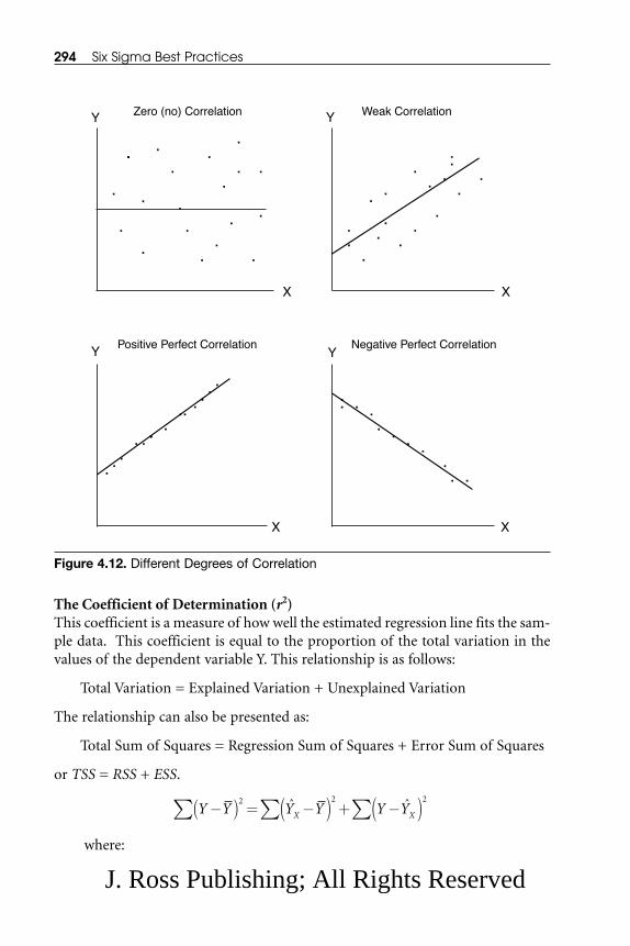
The Coefficient of Determination (r2)This coefficient is a measure of how well the estimated regression line fits the sam-ple data. This coefficient is equal to the proportion of the total variation in thevalues of the dependent variable Y. This relationship is as follows:
Total Variation = Explained Variation + Unexplained Variation
The relationship can also be presented as:
Total Sum of Squares = Regression Sum of Squares + Error Sum of Squares
or TSS = RSS + ESS.
where:
Y Y Y Y Y YX X−( ) = −( ) + −( )∑ ∑∑2 2 2ˆ ˆ
294 Six Sigma Best Practices
.
.
.
.
.
.
.
.
.
..
..
.
.
.
..
.
.
X
Y
.
.
..
..
..
.
.
..
.
.
.
.
.
X
Y
..
.. .
.
.
.
...
.
.
..
X
Y
.
..
.
. ..
.
.
. .
X
Y
Zero (no) Correlation Weak Correlation
Positive Perfect Correlation Negative Perfect Correlation
Figure 4.12. Different Degrees of Correlation
J. Ross Publishing; All Rights Reserved

Ys = Observed values of dependent variable Y
⎯Y = Mean of dependent variable
YX = Estimated value of Y for a given value of independent variable X
r2 = Explained variation/Total variation = RSS/TSS
Since, Total SS – ESS = RSS, therefore,
r2 = (TSS – ESS)/TSS = 1 – (ESS/TSS)
and a sample coefficient of determination (an alternate formula in relation to theregression equation):
where additional variables:
n = Sample size
c = Intercept of regression equation
m = Slope of regression equation
The Coefficient of Determination Adjusted [r2(Adj)]As defined earlier, r2 is adjusted for the degrees of freedom. If a variable is addedto an equation, r2 will almost always get larger, even if the added variable is of noreal value. Therefore, to compensate for this:
where:
m = Number of coefficients fit in the regression equation
rErrorSS n m
TSS n2
1=
−−
/( )
/( )
rc Y m XY nY
Y nY2
2
2 2=
+ −
−∑∑
∑
rY Y
Y Y
X2
2
21= −
−( )−( )
∑∑
ˆ
rY Y
Y Y
X2
2
2=
−( )−( )
∑∑
ˆ
Analyze 295
J. Ross Publishing; All Rights Reserved

The Coefficient of Correlation (r)The square root of the sample coefficient of determination, √r2, is a commonalternative index of the degree of association between two quantitative variables.The coefficient r takes on absolute values between 0 and 1. The positive or nega-tive value of r denotes a direct relationship or an inverse relationship between Xand Y, respectively. Therefore, when:
r = 0 � No correlationr = +1 � Perfect correlation between directly related variablesr = –1 � Perfect correlation between inversely related variables
The following is Pearson’s formula for calculating r without prior regressionanalysis (also known as Pearson’s Sample Coefficient of Correlation):
where:
Xs = Observed values of the independent variable
⎯X = Mean of independent variable
Ys = Observed associated values of the dependent variable
⎯Y = Mean of dependent variable
n = Sample size
Similarly, r(Adj) is the square root of the coefficient of determinationadjusted.
Example 4.13 (Continued): Applying the Coefficient of Determinationand the Coefficient of Correlation
Now analyze the coefficient of determination and the coefficient of correlation ofthe sample in Example 4.13. When developed in a linear regression equation:
r2 = 0.867 and r2(Adj) = 0.862 (this r2 is adjusted for degrees of freedom)
In other words, 86.2% of the total variation in Y (annual starting salary) wasobserved. Therefore, r(Adj) = 0.928, indicates that the annual starting salary isstrongly correlated with education level.
When using a quadratic regression equation:
r2 = 0.961, r2(Adj) = 0.958, and r(Adj) = 0.979
rXY nXY
X nX Y nY=
−
−( ) −( )∑
∑ ∑2 2 2 2
296 Six Sigma Best Practices
J. Ross Publishing; All Rights Reserved

This clearly shows that the quadratic equation is better fitted than the linear fit-ted equation.
Tools have been presented in this chapter to establish a qualitative relation-ship between the independent variables (Xs) and the dependent variable (Y). Thefollowing are the general comments related to the coefficient of determination andthe coefficient of correlation:
• As a regression equation is developed, the value of r2 will tell which ofthe three—linear, quadratic, or cubic—regression is a better-fit equa-tion. (If there is a poor or a no-linear relationship, then the value of r2
will be low, but this does not mean that there is no curvilinear rela-tionship.)
• Statisticians prefer to use r2 rather than r as a measure of associationbecause fairly high absolute values of r (e.g., r = 0.70) can give a falseimpression that a strong association exists between Y and X (but inthis case, r2 = 0.49; thus, the association of Y with X explains lessthan half of the variation of Y). Only at the extreme values of r,when r = ±1 or when r = 0 (under these situations, r = r2) does thevalue of r directly convey what proportion of the variation of Y isexplained by X.
• The correlation coefficient measures only the strength of a statisticalrelationship between two variables. A strong statistical relationshipbetween X and Y need not imply a causal relationship. Perhaps Ycauses X; perhaps X causes Y; or perhaps each is part cause/part effectof the other. Perhaps the two variables move together by pure chance.Therefore, the existence of a high-positive or -negative correlationbetween two variables that have no logical connection with oneanother is commonly known as a nonsense correlation or spurious cor-relation.
Exercise 4.6: Developing a Regression Equation
The quality group in a manufacturing company has collected sample data from awelding department and wants to establish a relationship between weld diameter(in inches) and the shear strength (in pounds) of weld. Develop a regression equa-tion; obtain the coefficient of determination and the coefficient of correlation.Provide data with comments. See Table 4.15 for the collected sample data.
Exercise 4.7: Determining an Estimated Regression Equation and theCoefficient of Correlation
A realtor wants to establish the relationship between the number of weeks housesare on the market prior to sale and the asking price. Sample data are provided in
Analyze 297
J. Ross Publishing; All Rights Reserved
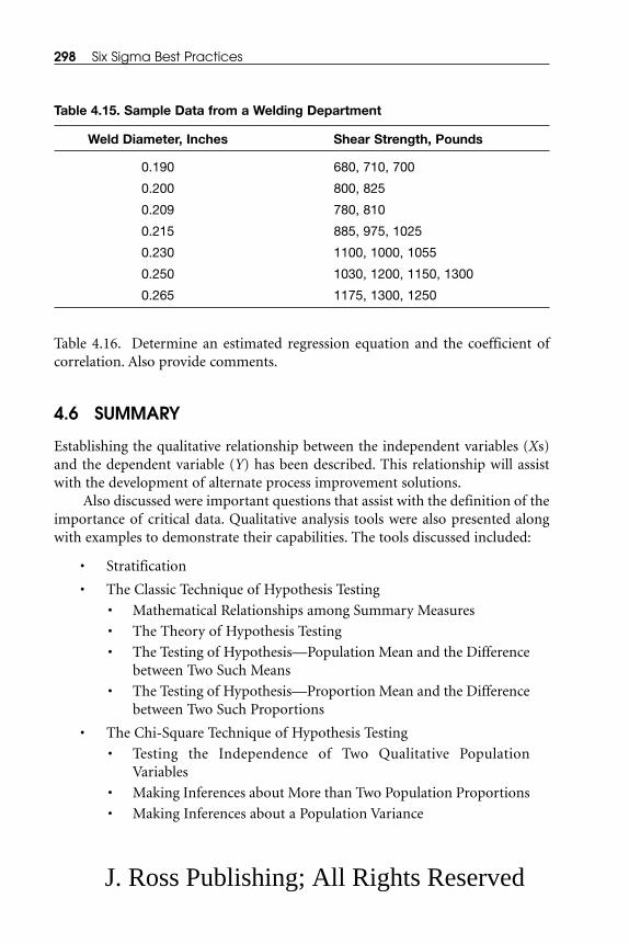
Table 4.16. Determine an estimated regression equation and the coefficient ofcorrelation. Also provide comments.
4.6 SUMMARY
Establishing the qualitative relationship between the independent variables (Xs)and the dependent variable (Y) has been described. This relationship will assistwith the development of alternate process improvement solutions.
Also discussed were important questions that assist with the definition of theimportance of critical data. Qualitative analysis tools were also presented alongwith examples to demonstrate their capabilities. The tools discussed included:
• Stratification
• The Classic Technique of Hypothesis Testing
• Mathematical Relationships among Summary Measures
• The Theory of Hypothesis Testing
• The Testing of Hypothesis—Population Mean and the Differencebetween Two Such Means
• The Testing of Hypothesis—Proportion Mean and the Differencebetween Two Such Proportions
• The Chi-Square Technique of Hypothesis Testing
• Testing the Independence of Two Qualitative PopulationVariables
• Making Inferences about More than Two Population Proportions
• Making Inferences about a Population Variance
298 Six Sigma Best Practices
Table 4.15. Sample Data from a Welding Department
Weld Diameter, Inches Shear Strength, Pounds
0.190 680, 710, 700
0.200 800, 825
0.209 780, 810
0.215 885, 975, 1025
0.230 1100, 1000, 1055
0.250 1030, 1200, 1150, 1300
0.265 1175, 1300, 1250
J. Ross Publishing; All Rights Reserved

• Performing Goodness-of-Fit Tests to Assess the Possibility thatSample Data Come from a Population Following a Specified Typeof Probability Distribution
• Analysis of Variance (ANOVA)—One-Way ANOVA
• Analysis of Variance Concept with Example
• Mathematical Model
• ANOVA Steps
• Regression and Correlation
• Definition of Key Terms
• Simple Regression Analysis
• Simple Correlation Analysis
Before proceeding to the next phase, Improve, of the DMAIC process, a projectteam should check the following:
• As information is processed and analyzed, identify gaps between thecurrent performance and the goal performance.
• Root cause analysis should have led to verifying and quantifying thecauses of variation and should have included:
• A list of possible causes or the sources of variation
Analyze 299
Table 4.16. Real Estate Sales Related Data
Asking Price, $K Weeks to Sale
40 6.5
198 8.6
160 6.8
199 10.6
200 14.0
250 15.0
201 8.6
260 15.0
250 12.1
360 19.0
280 9.0
240 12.5
220 9.5
400 27.0
J. Ross Publishing; All Rights Reserved

• A list and prioritizing of the issues or sources of variation byusing a Pareto chart
• Root cause analysis should have led to quantifying the gap/opportunity.
Questions may be used as a guide to determine the appropriate application toolfor information and process analysis:
• What does the information say about the performance of the businessprocess?
• Was any value-added, non-value added, and waste activities analysisdone to identify some of the gaps in the “as is” process map?
• Was a detailed process map created to reveal the critical steps of the“as is” process?
• What procedure was used in generating, verifying, and validating theprocess map?
• Was any additional useful information obtained through detailedsubprocess mapping?
• Were any cycle time improvement opportunities identified throughthe process analysis?
• Did the team think that additional information should have been col-lected during analysis?
• Which tool would best explain the behavior of output (dependent)variable(s) in relation to input (independent) variables?
Questions may also be used as a guide to quantify the gap/opportunity:
• What team is estimating the cost of poor quality?
• Is the process so broken that a redesign is required?
• If the team judges that the project is not a DMAIC process project,would the project lend itself to a DMADV project?
• What are the latest estimates of the financial savings/opportunities forthe improvement project? Where easy benefits can be obtainedthrough “quick fixes”?
• Was the project mission statement updated as the team went throughthe Analyze phase?
300 Six Sigma Best Practices
This book has free material available for download from theWeb Added Value™ resource center at www.jrosspub.com
J. Ross Publishing; All Rights Reserved

5
IMPROVE
The most important phase is Improve because this phase focuses on reducing theamount of variation found in a process. Reduction of variability is the solution tomany processes problems (e.g., in a manufacturing process). Although somereengineering programs promote the concept of tearing down the functional silosand rebuilding process groups from scratch, other businesses believe that theyshould start where they are organizationally and build on current successes andmodify current processes. These businesses strongly rely on the interwoven con-cepts of defect reduction, which encourage employees to rely more on each otherand cycle time reduction, which eliminates unnecessary, non-value-adding andwaste steps from processes.
Yet, Six Sigma requires more than a financial investment. Businesses musthave a plan, the required resources, the commitment of everyone, especially busi-ness leaders, and uncompromising metrics. Along with these elements, businesses
301
Define
Measure
Analyze
Improve
Control
6σ DMAIC
J. Ross Publishing; All Rights Reserved
302 Six Sigma Best Practices
must also set aggressive goals for a defined path and hold people accountable(both internal and external). Commonly utilized goals and commitments includehaving:
• A totally satisfied customer
• A commitment to a common language throughout the business
• A commitment to common and uniform quality measurement tech-niques throughout the business
• Improvement goals based on uniform metrics
• Goal-directed incentives for both employees and management
• Common training material on “why,” “how,” and “when” to achieve agoal
No one set of procedures can be used when following Six Sigma methodol-ogy. Every business is different and must consider its strengths and weaknessesand then leverage them accordingly.
Typically, a quantitative understanding of customer satisfaction can beachieved through surveys. These surveys should identify gaps between customerneeds and the company’s current performance levels. Then through benchmark-ing, the company’s core processes should be compared to another best-in-classperformer. This is useful in identifying the first layer of goals that are needed.Imagine that a company is performing at less than a four sigma level and that thecompetition is close to a six sigma level. Is the competition 2000 times better thanthe company? (A comparison such as this would certainly get the attention ofleaders of the business.) In a mathematical sense, six sigma is a known quality. Asimprovements are implemented, quality improves and everyone’s expectations goup. As customers’ perceptions about a business change, quality at the business isdriven to a level never before thought possible to achieve.
Businesses exist in which the corporate culture is fear-based and mistakes arenot tolerated. As a result, employees try to hide defects. Six Sigma programs canhelp these employees to minimize defects and the business will also flourish.
If one speaks with Six Sigma champions, they will identify numerous issuesto count, measure, benchmark, and improve regardless of the type of the business,e.g., whether it is a physician’s office or a storage space rental company. Within anybusiness, all types of variations can be found, e.g., from warehousing, security,and personnel policies to cafeteria management.
If any business is not improving, that business will eventually fail. Six Sigmais a philosophy of continuous improvement. As improvements are made, the busi-ness is driven in a direction of achieving its goals. Often improvement ideas comefrom customers; therefore, talk to customers and find out what they consider to
J. Ross Publishing; All Rights Reserved

be defects. Work on big defects first. Try to find out why they happen and how topermanently correct them.
Businesses that are satisfied with their current quality levels simply do notunderstand the real challenge of quality. Businesses that are satisfied should inves-tigate the defect levels their customers are experiencing as well as the internaldefects that cause rework, additional inspections, and higher product costs. Onlywhen a business fully assesses itself can improvements really begin.
Improvement strategies could include:
• The team applying the concept of process reengineering to determinethe solution (depending on team’s current level of process knowledgeand the additional information collected so far)
• In a systematic approach, the team examining the vital Xs (independ-ent variables) as they relate to the process to determine the bestapproach for developing a process/solution to produce an output tomeet customer needs
• The team determining the process/solution under the given con-straints (depending on the team’s total knowledge and understandingof the process/solution)
• The team incorporating different combinations of reengineering, sta-tistical, and quality tools
After giving consideration to the above list, the key step in the Improve phaseis to evaluate the team’s improvement strategy.
The team should begin the Improve phase by going through reengineering ofthe process/solution. The team should reengineer the current process and thengenerate alternatives to find the best process/solution under the given constraints.If the team does not have enough confidence to relate the independent variables(Xs) with the dependent variable (Y), then the team could set up a design ofexperiments (DOE) to develop a quantitative relationship between the inputs andthe output under the given constraints and modify the selected alternative accord-ing to the specific requirements of the process/solution. A DOE develops graphsand a regression equation that will allow the team to determine the best possiblecombination under the given constraints and operational settings.
It is possible that team’s project will include a combination of both types ofessential Xs (alternatives and factors). In this situation, the team would useimprovement strategies for the specific key Xs that may result in more than oneproposed process/solution. An improvement strategy flowchart will be presented(see Figure 5.1). Sources of variation include:
• A level of good communication with employees
• Employees knowing what they are supposed to do
Improve 303
J. Ross Publishing; All Rights Reserved

• Employees having access to business policies, guidelines, procedures,and quality standards—Employees must understand this informationand should be required to follow policies, procedures, etc. If employ-ees have issues with and/or are unclear about any policy, procedure,etc., they must have a contact source. Employees should understandthe consequences of failing to meet requirements.
• Employees having the requirement of sampling their work and havingthe time allocated for these activities—Employees should also berequired to record the results of their sampling.
• Supervisors maintaining individual employee performance records
• Employees being evaluated in quantitative terms in relationship tobusiness goals and having a correction mechanism in place to correctdeficiencies
Therefore, the first improvement activity could be process reengineering andthen developing improvement strategies for the factors and alternatives. Thischapter will discuss the following topics:
5.1 Process Reengineering
5.2 Guide to Improvement Strategies for Factors and Alternatives
5.3 Introduction to the Design of Experiments (DOE)
5.3.1 The Completely Randomized Single-Factor Experiment
5.3.2 The Random-Effect Model
5.3.3 Factorial Experiments
5.3.4 DOE Terminology
5.3.5 Two-Factor Factorial Experiments
5.3.6 Three-Factor Factorial Experiments
5.3.7 2k Factorial Design
5.3.7.1 22 Design
5.3.7.2 23 Design
5.4 Solution Alternatives
5.5 Overview of Topics
5.6 Summary
References
304 Six Sigma Best Practices
J. Ross Publishing; All Rights Reserved
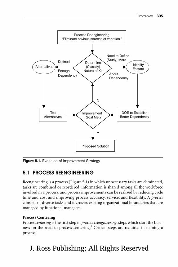
5.1 PROCESS REENGINEERING
Reengineering is a process (Figure 5.1) in which unnecessary tasks are eliminated,tasks are combined or reordered, information is shared among all the workforceinvolved in a process, and process improvements can be realized by reducing cycletime and cost and improving process accuracy, service, and flexibility. A processconsists of diverse tasks and it crosses existing organizational boundaries that aremanaged by functional managers.
Process Centering Process centering is the first step in process reengineering, steps which start the busi-ness on the road to process centering.1 Critical steps are required in naming aprocess:
Improve 305
Determine(Classify)
Nature of Xs
Defined
EnoughDependency
Alternatives
Need to Define(Study) More
AboutDependency
IdentifyFactors
Improvement Goal Met?
TestAlternatives
DOE to EstablishBetter Dependency
N
Y
Proposed Solution
Process Reengineering“Eliminate obvious sources of variation.”
Figure 5.1. Evolution of Improvement Strategy
J. Ross Publishing; All Rights Reserved

• Boundries—A typical process crosses existing organizational bound-aries:
– A “rule of thumb” is that if a process does not make more thantwo people angry, it is not a process.
– Many businesses simply rename a functional unit as a process.
– Process identification requires an ability to look horizontallyacross the whole organization, from the outside, rather than fromthe top down.
• Awareness—Include personnel levels from top executives to employ-ees at the lowest levels (e.g., the manufacturing floor of a productcompany) to ensure that all employees in the business are aware of theprocess and its importance to the business:
– Employees must recognize their process by name, must clearlyunderstand the inputs and outputs to the process, and must alsounderstand their relationship to the process.
– Process participants must link themselves to the whole process(up and down).
– Each participant is not to perform only his/her duties, but also towatch, understand, and support the process as necessary.
• Process Measurement—Every business must have a method for meas-uring a participant’s performance in completing the process.
• Process Management—Focus at the business must continue on allprocesses so that employees remain attuned to the needs of the chang-ing business environment:
– One-time improvements are of little value unless the entireprocess is addressed.
– A process-centered business must strive for ongoing processimprovement.
A process resource analysis is presented in Example 5.1.
Example 5.1: A Quick Process Resource Analysis
This business has a traditional, quite rigid hierarchical organization (Worker �Supervisor � Manager � Director � Vice President � . . .). Each process fol-lows the chain of command. For example, a customer makes a payment on hisinvoice. The employee receiving the customer’s payment is responsible for deter-mining if the payment was received “on-time” or if it is “late.” The accounts receiv-able department is responsible for determining whether the payment is for thecorrect amount or if it is not. If a data entry employee notices anything unusual,he/she must take the issue to his/her supervisor, then the supervisor takes the
306 Six Sigma Best Practices
J. Ross Publishing; All Rights Reserved

issue to his/her manager, etc. When a customer inquires about a payment, he/shehas to go through several employees to get all the information needed, a proce-dure that makes the customer unhappy. How should this business improve itspayment receiving process?
Solution:Business leadership must think “out of the box,” be creative, and establish fewerorganizational layers by cross-training employees in several areas:
• Contract interpretation
• Customer billing and how it is done
• Customer payments and how they should be made
• Correct payment amount
• Knowledge (limited) of account auditing
• Communication methods with field sales (about contract)
Easy access to customer accounts should be provided to customer service(customer contact) employees.
Process ActivitiesThe next step is analyzing process activities. Every process is a group of activitiesto achieve an objective. Process activities can be divided into three categories:
• Value-Adding Work—Work for which a customer is willing to pay
• Non-Value-Adding Work—Activities which create no value for thecustomer, but are required to get value-adding work done
• Waste—Work that neither adds any value for a customer nor isrequired to get the value-adding work done
A simple concept of process reengineering is to eliminate waste, minimizenon-value-adding work, and improve/modify/reprocess value-adding work.Businesses utilize significant amounts of resources to eliminate waste, which pro-vides benefits, but not enough benefits for a business in the competitive globalmarket. By simply eliminating waste activities, the business organization structureis unchanged. Non-value-adding work is also used as the “glue” that bindstogether value-adding work in a conventional process. Typically, non-value-adding activities fall into several categories:
• Checking • Supervising
• Reporting • Liaising
• Controlling • Reviewing
Improve 307
J. Ross Publishing; All Rights Reserved

Value-adding work is generally divided into very small tasks that require lim-ited knowledge and experience to complete. Supervisors/checkers are used tomonitor these activities (monitoring activities are non-value-adding work), e.g.,reviews, managerial audits, checks, approvals, etc. Although value-adding workersare generally less skilled and lower paid, their activities make a process complex.Their activities add expense. Adding complexity to a process makes the processerror-prone and difficult to understand. Although non-value-adding activitieshave been justified on the basis that they “make the process work,” they are also asource of:
• Errors • Inflexibility
• Misunderstanding • Rigidity
• Miscommunication • Telephone calls
• Squabbles • Headaches
• Reconciliation • Delay
Because simply eliminating these activities would not allow the process tofunction, it is therefore necessary to design non-value-adding work through reor-ganizing the value-adding work. This process is often called reengineering orprocess reengineering. Example 5.2 presents a situation in which specific employeequalifications are based on an identified process.
Example 5.2: Employee Qualifications for an Identified Process
Company XYZ has an opening for a customer service representative (CSR).2 Listthe qualities needed and knowledge requirements for this open position.
Solution:The responsibility of a CSR is to resolve a customer’s problem. A CSR must focuson the outcome rather than on any single activity. Therefore, a CSR must be pro-ficient in several distinct types of activities and must have knowledge of multipledisciplines. Specific qualities and requirements of a CSR include:
• Must be able to speak with customers and have the competency to usesophisticated software programs
• Must have sufficiently developed “people” skills
• Must grasp the essentials of a customer’s request for service
• Must have sufficient knowledge of company products and services torecommend solutions for customer problems
• Must have a sense of the “art and science” of working with companyresources
308 Six Sigma Best Practices
J. Ross Publishing; All Rights Reserved

• Must be able to judge priority situations and assign priorities cor-rectly to certain customers, e.g., during a busy time such as an emer-gency
• Must be able to train prospective employees for the CSR position,providing sufficient information about company products and serv-ices to allow new a CSR to recommend solutions to customers
If a selected candidate does not have these qualities, but is capable of learningthem, the company should provide all required training to the candidate beforehe/she begins to function as a CSR.
Analyzing the ProcessOnce the process reengineering team understands the basics of a process and thequality requirements of the participating employees, the next step is to analyze theprocess for reengineering. A process-centered job could have several characteris-tics, e.g.:
• Free of non-value-adding work
• Big and complex
• Covers a range of tasks. Requires job holder to understand the “bigpicture:”
– Business goals
– Customer needs
– Process structure
As non-value-adding work is eliminated (e.g., it is often minimized), the jobbecomes:
• Substantive
• Increasingly difficult (as a consequence of becoming substantive)
• Challenging
• Of higher intensity
and job responsibilities become:
• Results-oriented
• A route to personal autonomy
• Having the authority to make decisions
Reengineering jobs may have two types of employees—professionals andworkers. A professional is responsible for achieving results rather than performingtasks, e.g., attorneys, architects, accountants, physicians, etc. are responsible for
Improve 309
J. Ross Publishing; All Rights Reserved

achieving results. A professional’s “world view” consists of three categories—cus-tomer, results, and process. A professional must have a reservoir of knowledge andan appreciation for the application of this knowledge to different situations.Characteristics as a professional include:
• Has required education and training
• Does not necessarily work according to predefined instructions
• Is directed toward a goal and has been provided with significant lati-tude
• Must be a problem solver
• Must be able to cope with unanticipated and unusual situations with-out “running to management” for guidance
• Is a constant learner, not only in the classroom, but also in profes-sional life
• Must be competitive, with energy directed from inside the organiza-tion to outside
• Must have a professional career that concentrates on knowledge,capability, and influence
A worker recognizes personal responsibility based on three different cate-gories—boss, activity, and task, e.g, workers can be sales representatives, customerservice representatives, etc.
When an employee considers moving to a process-oriented environment, keyquestions come to mind:
• Will I succeed in this new type of work?
• What job title will I have?
• How and how much will I be paid?
• What are the prospects for future growth?
Process-centered work and a process-centered environment transform work-ers into professionals, with all the advantages and disadvantages this changeimplies.
A High-Level Listing of Process Reengineering Steps
Step 1. Define the Process to Be Analyzed:
• Identify the process that the team will analyze for improvement.
• Describe the process in enough detail for each activity to be identifiedas value-added, non-value-added, and waste.
310 Six Sigma Best Practices
J. Ross Publishing; All Rights Reserved

• Identify process starting and ending points.
Step 2. Map Process Flow:
• Prepare all step-by-step process flow maps by tracing all process stepsin sequence, as well as resources, functions, time, distance, etc.
Step 3. Define Process Activities:
• Define process flow, identifying each detailed step in the process andusing common sign conventions:
O Process/Operation
� Transport/Move
� Inspect
� Store
D Wait/Delay
Step 4. Analyze Throughput (Distance Traveled, Cycle Time):
• Some of the most important measurements that impact quality,inventory, cost, and customer satisfaction are measurements of thespeed with which a process is completed and in which the throughputis made.
Calculate value ratios and process documentation as presented in Figure 5.2:
Value-added work ratio = (Value-added work time)/(Total process cycletime)
Non-value-added work ratio = (Non-value-added work time)/(Totalprocess cycle time)
Waste ratio = (Waste time)/(Total process cycle time)
Improve 311
Value-AddedWork
Non-ValueAdded Work
Waste
Total Process Cycle Time
Figure 5.2. Graphic Presentation of a Process into Activity Classifications
J. Ross Publishing; All Rights Reserved
Summarize process cycle statistics as applicable:
• Activities statistics (value-added, non-value-added, waste)
• Distance traveled
• Delay/wait time
• Resources statistics
• Average cycle time
Generate ideas to eliminate waste and minimize non-value-added work:
• Utilize brainstorming concept to generate ideas.
Step 5. Test Feasibility of the Selected Idea:
• Because implementation of the selected idea is required, a feasibilitytest is critical.
Step 6. Implement Idea and Develop User Procedure Document:
• While implementing the selected idea, develop the user procedure-document.
Step 7. Record Results Achieved or Demonstrated:
• Summarize achieved results as well as expected results. If expectedresults are different, provide an explanation.
Exercise 5.1: Simplifying a Warehouse Material Receiving andStacking Process: Process Reengineering2
A warehouse layout is presented in Figure 5.3. Material receiving process flow-charts are provided in Figures 5.4 (parts A through G). Analyze the warehousingproblem, following the outline presented earlier. Propose an improved materialreceiving and stacking process.
Project guidance: This is not a typical warehouse such as would be found ina parts manufacturing facility warehouse (i.e., components). These warehousesare also not as technologically advanced as those found in a manufacturing facil-ity. The quality of material received in these warehouses also varies significantly.
Typically, there are two staging areas: one is on the receiving dock and the sec-ond is on the manufacturing side of the business just outside the warehouse.Generally, the material received needs to be quality-checked before it can bestacked in the warehouse. Most of the production material is a common type ofmaterial and it is supplied to several machines at the same time. Once material is
312 Six Sigma Best Practices
J. Ross Publishing; All Rights Reserved

retrieved from the warehouse for production, the material is staged in a secondstaging area. The material handling workforce then supplies the material toindividual production machines from the second staging area. The warehouselayout with the receiving dock and the two staging areas is presented in this exer-cise.
The duration of certain activities is provided as a range of time. In order tocalculate cycle time, use the average duration for these activities. While readingthe description of these activities, note that certain activities are a combination oftwo or more activities (as described earlier in Section 5.1, Process Reengineering).Classify these activities into value-added, non-value-added, and waste based onthe main action (function) performed during the defined activity time.
Improve 313
Receiving Dock AreaStage Received Material for Quality InspectionMaterial Transfers
for Stacking
StagingArea
Supply Material forMessage Production
Stacking De-staged Material
20 Ft
100 Ft
100 Ft
MessagingProducingFacility
Figure 5.3. Warehouse Layout
J. Ross Publishing; All Rights Reserved

314 Six Sigma Best Practices
Full/partial match of trucker’s list with WMS list
Warehouse Manager walks 100–300 ft; asks a forklift operator to unload truck
(5–10 min)
Forklift operator unloads the truck and stores material on receiving dock (45 min)
Forklift operator checks material and quantity as per supplier’s list (5 min)
Forklift operator signs slip, keeps one copy, and gives second copy to supplier’s truck
driver (5 min)
Forklift operator walks 200 ft; gives received material list to Quality Manager (5 min)
Quality Manager prints ordered material list from WMS and compares with supplier’slist
(10–15 min)
Quality Manager walks 200 ft to receiving dock staging area (5 min)
A
No match of trucker’s list with WMS list
Do not accept material
Trucker pulls truck from docking area
Drives truck back to supplier
Trucker backs up truck at warehouse dock
Presents material receipt to Warehouse Manager (5–15 min)
Warehouse Manager compares list against order quantities in Warehouse Management System (WMS) (5–10 min)
Figure 5.4 (Parts A to G). Warehouse Material Receiving and Stacking ProcessFlowchart
J. Ross Publishing; All Rights Reserved

Improve 315
B
CUnmatched material items
D
A
Supplier and WMS lists match
Quality Manager quality checks and tags all the received
material (10–20 min)
Supplier and WMS lists have partial match
Matched material items
Quality Manager quality checks and tags material items (5–15 min)
Accepted–all received material items
Warehouse Manager receives material items in WMS; finds storage locations in warehouse and writes locations
on list (15–20 min)
Warehouse Manager writes e-mail to supplier about material quality (5 min)
Warehouse Manager walks 200–300 ft, passes material list to forklift operator, and asks operator to store material
in warehouse (5– 5 min)
Forklift operator moves material from dock staging area into warehouse as per assigned locations and updates material in storage locations through radio frequency
handheld unit (50–70 min)
Forklift operator walks 200 ft; passes material list to Warehouse Manager (5 min)
Warehouse Manager checks material status in WMS
Receiving and stacking process complete
Quality Manager walks back to Warehouse Manager’s office (200 ft); passes on material quality list (5 min)
B
B1
Figure 5.4B.
Figure 5.4C.
J. Ross Publishing; All Rights Reserved

316 Six Sigma Best Practices
Partially Accepted–all received material items
Warehouse Manager receives material items in WMS; finds storage locations in warehouse and writes locations on list
(15–20 min)
Warehouse Manager writes an e-mail to supplier about material quality and expects supplier to pick-up rejected material by following working day
(5 min)
Warehouse Manager walks 200–300 ft; passes material list to forklift operator;
asks operator to store accepted material in warehouse (5–15 min)
Forklift operator moves only accepted material from dock staging area into
warehouse as per assigned locations and updates material in storage locations with
radio frequency handheld unit (50–70 min)
Forklift operator walks 200 ft; passes material list to Warehouse Manager
(5 min)
Warehouse Manager checks material status in WMS
Supplier truck arrives the following working day; Warehouse Manager asks
forklift operator to load rejected material in truck and get trucker’s signature for
material received (15–50 min)
Receiving and stacking process complete
B1
Figure 5.4D.
J. Ross Publishing; All Rights Reserved

Improve 317
Accepted–all matched material items
Warehouse Manager received material items in WMS; finds storage locations in warehouse and writes locations on list
(15–20 min)
Warehouse Manager writes e-mail to supplier about material quality (5 min)
Warehouse Manager walks 200–300 ft; passes material list to forklift operator and
asks operator to store material in warehouse (5–15 min)
Forklift operator moves material from dock staging area into warehouse as per
assigned locations and updates material in storage locations with radio frequency
handheld unit (30–70 min)
Forklift operator walks 200 ft; passes material list to Warehouse Manager
(5 min)
Warehouse Manager checks material status in WMS
Receiving and stacking process complete
C
C1
Quality Manager walks back to Warehouse Manager’s office (200 ft); passes material quality
list (5 min)
Figure 5.4E.
J. Ross Publishing; All Rights Reserved

318 Six Sigma Best Practices
Partially Accepted — all matched material items
Warehouse Manager receives material items in WMS; finds storage locations in warehouse and
writes locations on list (15–20 min)
Warehouse Manager writes e-mail to supplier about material quality and expects supplier to pick-
up rejected material by following working day (5 min)
Warehouse Manager walks 200–300 ft; passes material list to forklift operator and asks operator to
store accepted material in warehouse (5–15 min)
Forklift operator moves only accepted material from dock staging area into warehouse as per
assigned locations and updates material in storage locations with radio frequency handheld unit
(30–70 min)
Forklift operator walks 200 ft; passes material list to Warehouse Manager (5 min)
Warehouse Manager checks material status in WMS
Supplier truck arrives the following working day; Warehouse Manager asks forklift operator to load
rejected material in truck and get trucker’s signature for material received (15– 50 min)
Receiving and stacking process complete
C1
Figure 5.4F.
J. Ross Publishing; All Rights Reserved

5.2 GUIDE TO IMPROVEMENT STRATEGIES FOR FACTORSAND ALTERNATIVES
As the team went through the Analyze phase of identifying the relationshipbetween independent variables (Xs) and the dependent variable (Y), along withapplying the concept of process reengineering, the team would decide whether theY = f(X) relationship has been defined enough or not. Two identified conditionswill be discussed:
Condition 1. Dependency has been sufficiently defined so that the team candevelop alternatives:
• Various independent scenarios can be developed that must be tested.
• Risk assessment will be needed for each scenario.
• Alternatives will need testing either through pilots or through simu-lation.
• Alternatives will need evaluation, with selection of the best alternativeunder the given constraints
Possible issues include:
Improve 319
Unmatched material items
Quality Manager (because these are not ordered material items) makes no quality check on these
material items
Warehouse Manager writes e-mail to supplier about unordered material and expects supplier to pick-up material by following working day (5 min)
Supplier truck arrives the following working day; Warehouse Manager asks forklift operator to load
unordered material in truck and get trucker’s signature for material received (15–50 min)
Receiving and stacking process complete
D
Figure 5.4G.
J. Ross Publishing; All Rights Reserved
• Process Flow—Optimize process flow issue under the given/modi-fied/improved constraints.
• Lack of Standardized Process/Operation—Standardize the process asmuch as possible.
• Specific Problem Identified—Develop a good practical solution to theproblem.
Possible alternatives include:
• Brainstorming ideas
• Benchmarking and best practices
• Mistake checking (monitoring)
• Making pilot tests
• Process mapping and reengineering
• Process simulation
Condition 2. Dependency has not been sufficiently defined. The team will need tofurther define (or study) the dependency of Y on factor Xs. Possible methods todefine dependency include:
• Run simulation or design of experiment (DOE).
• Optimize significant factors under the given constraints.
• Develop a prediction equation/mathematical model.
Factors can be continuous or discrete, but risk assessment is critical in both sit-uations.
• If factors are continuous, and the team needs to develop a model topredict process behavior and to solve the issue, team will need todevelop a mathematical model.
• If factors are discrete, and can be set at different levels, the team willneed to determine the best possible combination with identified fac-tor values (levels) under the given constraints.
When dependency has not been defined sufficiently, two tools are commonlyused:
• Design of experiments (DOE)
• Simulation
If the project team is not confident about the relationship between independ-ent variables and the dependent variable, then the next step is to design and con-duct a DOE (see Section 5.3, Introduction to the Design of Experiments).
320 Six Sigma Best Practices
J. Ross Publishing; All Rights Reserved

Before moving on to the next section, consider the four scenarios in Exercise5.2. These scenarios have been developed to identify an improvement strategy foreach scenario.
Exercise 5.2: Identifying Factors and Alternatives and DeterminingImprovement Strategies
Instructions: In the following scenarios, determine if each scenario is based on fac-tors or alternatives. Determine the improvement strategy that should be imple-mented.
Case 1. To Improve Average Patient Treatment Time in an Emergency RoomA Six Sigma team has completed a project to improve treatment time in an emer-gency department of a hospital. The team identified critical Xs for fast treatmentas:
• Attending physican
• Diagnostic equipment
The team modeled the relationship of these factors to average treatment timerequired to treat emergency room patients. They used two-way ANOVA (analysisof variance) with existing data to develop a useful model. The team used themodel to assess the impact of each factor on treatment time and to assess intera-tion of the factors with each other. This type of analysis helped them to developan alternate solution.
� Factors
or
� Alternatives?
Any improvement strategy?
Case 2: To Improve Product Demand that Will Lead to Increased RevenueA Six Sigma team project has examined methods to improve demand for a prod-uct, which would increase revenue. To attract potential customers, the teamdecided to educate them about the products that are offered by the company. Theteam also tried to identify key Xs to improve demand:
• Product price
• Customer income
• Customer taste
To solve the problem, the team needed to model the relationship of these keyXs to product demand and determine which key Xs would eventually increase rev-
Improve 321
J. Ross Publishing; All Rights Reserved

enue to the level that is required to meet the target of business leadership. Theyused multiple regression analysis with historical data to develop a useful model.The team used the model to assess the relative impact of each key X on demandand then developed an alternative solution based on the analysis of information.
� Factors
or
� Alternatives?
Any improvement strategy?
Case 3. To Reduce Process Variation and Cycle Time for AssemblingElectromechanical ProductsA Six Sigma team project is to reduce process variation, assembly, and test cycletime for electromechanical products. Work flow analysis showed that four sepa-rate processes had evolved in different assembly and test areas as a result ofupgraded products. However, existing processes had not been documented orstandardized. Frequent delays occurred from part shortages as well as from excessinventory of the wrong parts.
After observing the process for each model, the team decided to develop ageneric work flow diagram for all products and, subsequently, to modify this com-mon process to fit the individual products. The team worked with process engi-neers from each product group to build and validate a generic work flow processchart. Then, the cross-functional process team developed, tested, and imple-mented process instructions that were tailored to each product being assembledand tested.
� Factors
or
� Alternatives?
Any improvement strategy?
Case 4. To Increase the Number and Quality of Service Contract Leads for aService-Providing BusinessA Six Sigma team has as a project to increase the number and quality of serviceleads for a service-providing business. The team reviewed service calls from theprevious year. They determined that the business lost a large number of desirablecustomers to competitors due to prospective customers receiving incompleteservice information. The team decided to attract potential customers by provid-ing them with better information about the services that are available. They devel-oped methods to accomplish this:
322 Six Sigma Best Practices
J. Ross Publishing; All Rights Reserved
• Mass mailing of printed service literature
• Testomonials from existing customers
• Calls to customers of competitors
• Advertising a quick service-response time
Evaluation of data from the trials showed that advertising a quick service-response time generated the most service business.
� Factors
or
� Alternatives?
Any improvement strategy?
5.3 INTRODUCTION TO THE DESIGN OF EXPERIMENTS (DOE)
If the premise that new knowledge is most often obtained by careful analysis andthat interpretation of data is accepted, then paramount is giving considerablethought and effort to planning data collection so that maximum information isobtained with the least expenditure of resources.
What is an experiment? Different definitions are available for the wordexperiment. For our purposes, consider an experiment to be “a planned inquiry toobtain new facts or to confirm or deny the results of previous experiments, wheresuch inquiry would aid the team in the decision process.” Some conducting exper-iments might comment that the results of this “experiment” are remarkably well-behaved and that they exhibit little of the variation with which they have tocontend. However, these results will serve the purposes of the team. For example,the objective of this “experiment” is to compare the speed of two machines. Theobjective can be stated in two ways: “Is there any difference in speed?” and “To testthe hypothesis that there is no difference in speed.” The second stated objective,which is related to the first, is to estimate the size of the difference in speed.Almost all experiments are carried out for one or both of these objectives: testingthe hypothesis and estimating the differences in the effect of various treatments.
Experiments are performed in all disciplines—engineering, scientific, finan-cial, and marketing—and are a major part of the discovery and learning process.Decisions that are made based on the results of an experiment are dependent onhow the experiment was conducted. Therefore, the design of an experiment(DOE) plays a major role in the problem solution.
What is a design of an experiment? A DOE is a formal plan for conductingan experiment. It includes the choice of responses, factors, levels, blocks, and
Improve 323
J. Ross Publishing; All Rights Reserved

treatments and also allows for planned grouping, randomization, repetition,and/or replication. DOE identifies how factors (independent variables, Xs) indi-vidually and in combination affect the process and its output (dependent vari-ables, Ys). A DOE develops a mathematical relationship and determines the bestconfiguration or combination of independent variables, Xs. A DOE is a most effi-cient tool.
Analysis of the results from a DOE is not difficult, especially if computer-based tools such as MINITAB software are utilized. Because computing technol-ogy is inexpensive and easily available, computer-based tools are the best way toconduct experiments. Remember: The best analysis in the world cannot rescue apoorly designed experiment.
DOE accomplishes the following:
• Identifies significant Xs and also helps the team to narrow a list to themost potential Xs and their impact on the process.
• Develops a quantitative relationship between Xs and Ys.
• Identifies interactions among Xs and if any interactions affect Ys,helping the team in their decision-making process.
• Identifies the best values of Xs to optimize Ys for the defined processconstraints.
5.3.1 The Completely Randomized Single-Factor Experiment Begin with considering how an experiment would be designed for testing the dif-ferential effect of raw material of the same specifications from different supplierson the output product quality. Although this concept has already been discussedin Chapter 4 (Analyze), some additional mathematical detail will now be given.
Suppose there are m different suppliers of the same material that are to becompared (a single-factor treatment). The product output for the raw material(treatments) of each of the m suppliers is a random variable. Observed data arepresented in Table 5.1, where:
Yij = the jth observation (output product quality) taken under treatment i(material supplier i)
i = 1, 2, 3, …, m
j = 1, 2, 3, …, n (number of observations)
Observations presented in Table 5.1 are the linear statistical model, where:
Yij = μ + τi + εij
μ = Overall mean (parameter common to all treatments)
324 Six Sigma Best Practices
J. Ross Publishing; All Rights Reserved

τi = ith treatment effect (parameter associated with the ith treatment)
εij = Random error component
For hypothesis testing, the model errors are assumed to be normally andindependently distributed random variables with mean zero and variance σ2
[abbreviated as NID(0, σ2)]. The variance σ2 is assumed constant for all levels ofthe factor. The above model equation is known as the one-way classification analy-sis of variance (ANOVA) because only one factor is investigated.
In the fixed-effect model, the treatment effects τ1 are usually defined as devia-tions from the overall mean, so that:
Therefore, to test the equality of the m treatments (material suppliers) effects,the appropriate hypotheses are:
H0: τ1 = τ2 = … = τm = 0
H1: τi ≠ 0 for at least one i
The process logic is the same as that in Chapter 4, Analyze.
5.3.2 The Random-Effect Model In several situations, the factor of interest could be a large number of possible lev-els. Suppose a Six Sigma team was interested in drawing conclusions about theentire population of factor levels. If the team had selected m of these levels fromthe population of factor levels, then the team could say that the factors were ran-dom factors. Since the levels of the factor actually used in the experiment werechosen randomly, the conclusions reached would be valid for the entire popula-
τ ii
m
=∑ =
1
0
Improve 325
Table 5.1. Data for One-Way Classification ANOVA
Treatment, i Observation, j(Supplier Material) (Output Product Quality) Totals Averages
1 Y11 Y12 … Y1n Y1. ⎯Y1
|
m Ym1 Ym2 …Ymn Ym. ⎯Ym
J. Ross Publishing; All Rights Reserved

tion of factor levels. The team would assume that the population of factor levelsis either of infinite size or large enough to be considered infinite.
The linear statistical model uses the same equation, but in this case, it is calledthe components of variance or the random-effect model:
Yij = μ + τi + εij
where:
τi and εij are independent random variables
If the variance of τi is στ2, then the variance of any observation is
V(Yij) = στ2 + σ2
where:
στ2 and σ2 are variance components
In order to test hypotheses in this model, requirements are that:
{εij} are NID(0, σ2) and
{τi} are NID(0, στ2) and that:
τi and εij are independent
The assumption, that the {τi} are independent random variables, implies thatthe unusal assumption of:
from the fixed-effect model, does not apply to the random-effect model.
The sum of squares identity is the same:
SSTotal = SSTreatment + SSError
and the appropriate testing hypotheses are:
H0: στ2 = 0
H1: στ2 > 0
τ ii
m
=∑ =
1
0
326 Six Sigma Best Practices
J. Ross Publishing; All Rights Reserved

• Null hypothesis, if στ2 = 0, all treatments are identical.
• Alternate hypothesis, if στ2 > 0, then there is variability between treat-
ments.
(SSError/σ2) ~ Chi-square distribution with (N – m) degrees of freedom, where
N = total number of observations, m = total number of treatments
and under the null hypothesis,
(SSTreatment/σ2) ~ Chi-square distribution with (m – 1) degrees of freedom
Since both random variables are independent, therefore, under the nullhypothesis, the ratio:
where:
F ~ df((m – 1), (N – m))
Usually estimating the variance components (σ2 and στ2) in the model is
needed. The procedure used to estimate σ2 and στ2 is called the analysis of vari-
ance. The procedure consists of equating the expected mean squares to theirobserved value in the analysis of variance table and solving for the variance com-ponents. When equating observed and expected mean squares in the one-wayclassification random-effect model, the following is obtained:
MSTreatment = σ2 + nστ2
where:
n = Number of replicates and
MSError = σ2
Therefore, the estimators of the variance components are
�σ2 = MSError
FMS
MSTreatment
Error
0 =
F
SS
m
SS
N m
Treatment
Error
0
1=
−
⎛
⎝⎜⎜⎜
⎞
⎠⎟⎟⎟⎟
−
⎛
⎝⎜⎜⎜
⎞⎞
⎠⎟⎟⎟⎟
Improve 327
J. Ross Publishing; All Rights Reserved

�στ2 = (MSTreatment – MS Error)/n and
�V(Yij) = �στ2 + �σ2
For unequal sample size, replace n in the above equation with n0,
Note: Sometimes the analysis of variance method produces a negative esti-mate of the variance component. Since variance components are by definitionnon-negative, a negative estimate of the variance component is troublesome.Some solutions include:
• Accept the estimate and use it as a proof that the true value of thevariance component is zero, assuming that sampling variation hascreated the negative estimate. This has some intuitive appeal, but itwill disturb the statistical properties of other estimates.
• Reestimate the negative variance component with a method thatalways yields non-negative estimates.
• Consider the negative estimate as evidence that the assumed linearmodel is not correct. Another study with an assumption of a moreappropriate model may be needed.
This concept will now be presented in Example 5.3.
Example 5.3: A Single-Factor Experiment Involving the Random-EffectModel
A company that manufactures window screen materials weaves screen material ona number of looms. The company is interested in determining loom-to-loomvariability in tensile strength of the screen material. Tensile strength of the screenmaterial has been varying between 86 and 104 psi, with an average tensile strengthof 95 psi. The minimum requirement is 90 psi. A process engineer has redesignedthe production process to reduce variation in the tensile strength to between 90and 100 psi.
To validate the production process, the process engineer has set up an exper-iment to investigate the tensile strength of the screen material. The process engi-neer selects four looms at random and makes four strength determinations on
nm
nn
ni
ii
m
ii
mi
m
0
2
1
1
1
1
1=
−−
⎡
⎣
⎢⎢⎢⎢⎢⎢
⎤
⎦
⎥⎥⎥=
=
=
∑
∑∑ ⎥⎥
⎥⎥
328 Six Sigma Best Practices
J. Ross Publishing; All Rights Reserved
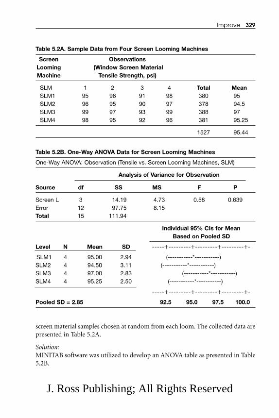
screen material samples chosen at random from each loom. The collected data arepresented in Table 5.2A.
Solution:MINITAB software was utilized to develop an ANOVA table as presented in Table5.2B.
Improve 329
Table 5.2A. Sample Data from Four Screen Looming Machines
Screen ObservationsLooming (Window Screen Material Machine Tensile Strength, psi)
SLM 1 2 3 4 Total MeanSLM1 95 96 91 98 380 95SLM2 96 95 90 97 378 94.5SLM3 99 97 93 99 388 97SLM4 98 95 92 96 381 95.25
1527 95.44
Table 5.2B. One-Way ANOVA Data for Screen Looming Machines
One-Way ANOVA: Observation (Tensile vs. Screen Looming Machines, SLM)
Analysis of Variance for Observation
Source df SS MS F P
Screen L 3 14.19 4.73 0.58 0.639Error 12 97.75 8.15Total 15 111.94
Individual 95% CIs for MeanBased on Pooled SD
Level N Mean SD -----+---------+---------+---------+-
SLM1 4 95.00 2.94 (-----------*-----------) SLM2 4 94.50 3.11 (-----------*-----------) SLM3 4 97.00 2.83 (-----------*-----------) SLM4 4 95.25 2.50 (-----------*-----------)
-----+---------+---------+---------+-
Pooled SD = 2.85 92.5 95.0 97.5 100.0
J. Ross Publishing; All Rights Reserved

The F table value at α = 0.05, and df (3, 12) is equal to 3.49. Since Fcalculated <Ftable, therefore, the manufacturing process on these loom machines is not signif-icantly different.
The process standard deviation can be estimated as follows:
�στ2 = (MSTreatment – MS Error)/n
= (4.73 – 8.15) / 4
= –0.855�V(Yij) = �στ
2 + �σ2
= – 0.855 + 8.15
= 7.295
The estimated process standard deviation is:
= √(7.295)
= 2.7
The pooled standard deviation (SD) using MINITAB software is 2.85 as shown inan ANOVA table (see Table 5.2B).
5.3.3 Factorial ExperimentsWhen there are several interesting independent factors (Xs) for an experiment, afactorial design should be used. Factors vary together in these experiments. A fac-torial experiment indicates that in each complete trial or replicate of the experi-ment, all possible combinations of the levels of the factors are investigated.
The following discussion will illustrate a simple factorial experiment. Thereare two factors P and Q, with p levels of factor P and q levels of factor Q. Eachreplicate would have all pq treatment combinations. The effect of a factor isdefined as the change in response produced by a change in the level of this factor.This change is called the main effect because it refers to the independent factors inthe study. Consider the data related to P and Q factors as presented in Table 5.3.
The main effect of factor P is the average difference of outputs between thelevels (P2 – P1) or:
P = ((35 + 45) / 2) – ((15 + 25) / 2)
= 20
i.e., changing factor P from level 1 to level 2 creates an average response increaseof 20 units. Similarly, the main effect of factor Q is:
ˆ ˆ ( )σY ijV Y=
330 Six Sigma Best Practices
J. Ross Publishing; All Rights Reserved

Q = ((25 + 45) / 2) – ((15 + 35) / 2)
= 10
Sometimes, there is a difference in response between the levels of one factorand the levels of the other factor. Sample data are presented in Table 5.4. At Q1
level of Q, while changing P from level from P1 to P2, the P effect is:
P = 35 – 15 = 20
Similarly, at Q2 level of Q, while changing P level from P1 to P2, the P effect is:
P = 0 – 25 = –25
and the main effect of P is:
P = ((35 + 0)/2) – ((15 + 25)/2)= –2.5
The impact is greater when the effect of P is examined at different levels offactor Q, but the main effect is not that significant. Therefore, knowledge of thePQ interaction is more useful than knowledge of the main effect. Sometimes a sig-nificant interaction may hide the significance of main effects. The data presentedin Tables 5.3 and 5.4 are also presented graphically in Figures 5.5A and 5.5B,respectively.
Improve 331
Table 5.3. Factorial Experiment with Two Factors
Factor Q
Factor P Q1 Q2
P1 15 25
P2 35 45
Table 5.4. Factorial Experiment with Interaction
Factor Q
Factor P Q1 Q2
P1 15 25
P2 35 0
J. Ross Publishing; All Rights Reserved

5.3.4 DOE TerminologyDefinitions of commonly used terms include:
• Independent Variable—Independent variables, variable Xs, are com-monly known as factors. A factor may be discrete or continuous. If thefactor is discrete, factor levels would naturally exist, which would be
332 Six Sigma Best Practices
0
10
20
30
40
50
.
Factor P
Obs
erva
tion
Q2
Q2
Q1
Q1
P1 P2
0
10
20
30
40
.
.
Factor P
Obs
erva
tion
Q2
Q2
Q1
Q1
P1 P2
Figure 5.5A. Two-Factors Experiment with No Interaction (Using Table 5.3 Data)
Figure 5.5B. Two-Factors Experiment with Interaction (Using Table 5.4 Data)
J. Ross Publishing; All Rights Reserved

used in the experiment. If a factor is continuous, it must be classifiedinto two levels: low and high.
• Dependent Variable—The value of the dependent variable is assumedto be unknown and is symbolized by Y. The dependent variable isoften called the response variable.
• Factor—A factor is an input in the experiment and could be a con-trolled or an uncontrolled variable whose impact on a response isbeing studied in the experiment. A factor might be qualitative (e.g.,different operators, machine types) or might be quantitative (e.g., dis-tance in feet or miles, time in minutes).
• Level—Levels are the input values of a factor being studied in anexperiment. Levels should be set far enough apart that effects on thedependent variable Y can be detected. Levels are generally referred toas “–1” and “1.” A level is also known as a treatment. Therefore, eachlevel is a treatment.
• Factorial k1 × k2 × k3 …—Factorial k1 × k2 × k3 … is a basic descrip-tion of a factorial experiment design. Each k represents a factor andthe value of k is the number of levels of interest for that factor, e.g., a3 × 2 × 2 design indicates that there are three input variables (factors).One input has three levels and the other two have two levels.
• Experimental Run (Test Run)—An experimental run is one or moreobservations of the output variable for a defined level of input vari-able(s).
• Treatment Combination—Identifying the experiment runs using a setof specific levels of each input variable is known as treatment combi-nation. A full experiment uses all the treatment combinations for allthe factors, e.g., a 3 × 2 × 2 factorial experimental design will have 12possible treatment combinations in the experiment.
• Repetition—Repetition is running more than one experiment consec-utively using the same treatment combinations.
• Replication—In replication, the same experimental setup is usedmore than once with no change in the treatment levels to collect morethan one data point. Replicating an experiment allows the user to esti-mate the residual or experimental error.
• Balanced Design—In a balanced design, each level for any one factoris repeated the same number of times for all possible combination lev-els of the other factors, e.g., a factorial design of two factors (A and B)and two levels (–1, 1) will have four runs as shown in Table 5.5.
Improve 333
J. Ross Publishing; All Rights Reserved

• Unbalanced Design—A designed experiment that does not meet thecriteria of balanced design is known as an unbalanced design, e.g., adesign in which each experimental level for any one factor is notrepeated the same number of times for all possible levels of the otherfactors.
5.3.5 Two-Factor Factorial ExperimentsThe easiest type of factorial experiment is considered to be a situation in whichthere are only two factors (e.g., A and B). Assuming “a” levels of factor A and “b”levels of factor B, let there be n replicates of the experiment and let each replicatecontain all ab treatment combinations. The two-factor factorial is a completelyrandomized design in which any observation may be described by the linearmodel that follows:
Yijk = μ + τi + βj + (τβ)ij +εijk
where:
Yijk = ijth observation in the kth replicate
i = 1, 2, …, a
j = 1, 2, …, b
k = 1, 2, …, n
μ = Overall mean effect
τi = Effect of the ith level of factor A
βj = Effect of the jth level of factor B
(τβ)ij = Effect of interaction between A and B
εijk = A NID(0, σ2) random error component
Because two factors are under study, the process used is called a two-wayanalysis of variance. Therefore, to test:
334 Six Sigma Best Practices
Table 5.5. Factorial Design Runs for 2 × 2
Run Factors � A B
1 –1 –12 1 –13 –1 14 1 1
J. Ross Publishing; All Rights Reserved

H0: τi = 0 (no row factor effects)
H0: βj = 0 (no column factor effects)
H0: (τβ)ij = 0 (no interaction effects)
This would lead to an ANOVA table for the two-way classification with fixed-effect model as presented in Table 5.6.
F distribution with:
• Numerator degrees of freedom = The number of degrees of freedom for the numerator mean square
• Denominator degrees of freedom = ab(n – 1)
Detailed statistical logic may be found in any DOE textbook.
Commonly followed steps to set up and run an experiment include:
Step 1. Select project’s dependent variable, Y.
Step 2. Select independent variables, Xs.
Step 3. Select the test levels for each independent variable (X).
Step 4. Perform risk analysis.
Step 5. Select the design and set up the experiment.
Step 6. Run the experiment and collect data.
Step 7. Analyze data.
Step 8. Perform statistical testing, e.g., hypothesis testing, predictionmodel, etc.
Step 9. Draw conclusions and complete confirmation runs.
This concept is explained by Example 5.4.
Improve 335
Table 5.6. ANOVA Table for a Two-Way Classification, Fixed-Effect Model
Source of Sum of Degrees ofVariation Squares Freedom Mean Square F0
A treatments SSA a – 1 MSA = SSA/(a – 1) MSA/MSE
B treatments SSB b – 1 MSB = SSB/(b – 1) MSB/MSE
Interaction SSAB (a – 1)(b – 1) MSAB = SSAB/(a – 1)(b – 1) MSAB /MSE
Error SSE a b(n – 1) MSE = SSE/(a b)(n – 1)
Total SST abn - 1
J. Ross Publishing; All Rights Reserved

Example 5.4: A Two-Factorial Experiment
This experiment involves a storage battery used in the launching mechanism of ashoulder-fired ground-to-air missile. Three material types are used in the test bat-tery plates. The objective is to recommend a battery that is relatively unaffected byambient temperature. The output response from the battery is expected to bemaximum voltage. Three temperature levels were used in the test, and a factorialexperiment with four replications was designed to run the experiment. The col-lected data are presented in Table 5.7A (the body of the table is maximum voltagedata or battery output response). As a hired consultant, what plate material wouldyou recommend?
Solution:
• Dependent variable—Battery output response in voltage
• Independent variables—Material and temperature (three levels foreach)
The MINITAB software tool is used to analyze the relationship between inde-pendent and dependent variables through the factorial design. Assuming that theindependent variables are fixed, test:
H0: τi = 0 (no material effects)
H0: βj = 0 (no temperature effects)
H0: (τβ)ij = 0 (no interaction effects)
Divide the corresponding mean square by mean square error. Each of theseratios would follow an F distribution with degrees of freedom given in Table 5.6.An ANOVA table was developed with MINITAB software (Table 5.7B).
336 Six Sigma Best Practices
Table 5.7A. Collected Data: 3 × 3 Factorial Experiment with Four Replications
Temperature (°F)
Material Low Medium High
1 131 150 35 41 21 6975 175 79 76 81 59
2 149 187 135 123 26 69160 127 107 116 58 45
3 137 109 173 121 95 105170 159 151 140 83 61
J. Ross Publishing; All Rights Reserved

Since table F0.05,2,27 = 3.35 and F0.05,4,27 = 2.73, the conclusion is that materialtype and temperature levels affect battery output voltage (a significant interac-tion); futhermore, there is also an interaction between these factors. A graph of thebattery output voltage averages vs. the type of battery plate material at three dif-ferent temperatures (low, medium, and high) has been plotted in Figure 5.6A.
Plate Material 3 provides a higher voltage output for a wider temperaturerange. There is an interaction between Materials 2 and 3 at a low temperature andbetween Materials 1 and 2 at a high temperature.
Model Adequacy CheckingResiduals from a factorial experiment are important in assessing model adequacy.Residuals are the differences between the observations and the corresponding cellaverages:
Eijk = Yijk – ⎯Yij
The normal probability plot of the voltage residuals is shown in Figure 5.6B.This plot has tails that do not fall exactly along a straight line passed through thecenter of the plot. This indicates that there are some potential problems with thenormality assumption, but that the deviation from normality does not appearsevere.
Improve 337
Table 5.7B. ANOVA Information for 3 × 3 Factorial Experiments for Example 5.4
Factorial Design: General Factorial Design
Factors: 2 Factor Levels: 3, 3Runs: 36 Replicates: 4
General Linear Model: Battery Voltage vs. Material, Temperature (°F)Factor Type Levels Values
Material Fixed 3 1 2 3Temperature Fixed 3 1 2 3
Analysis of Variance for Battery, using Adjusted SS for Tests
Source df Seq SS Adj SS Adj MS F P
Material 2 11084.7 11084.7 5542.3 8.80 0.001Temperature (°F) 2 38280.5 38280.5 19140.3 30.40 0.000Material/ 4 9471.3 9471.3 2367.8 3.76 0.015
Temperature (°F)Error 27 16998.5 16998.5 629.6
Total 35 75835.0
J. Ross Publishing; All Rights Reserved

A plot of the residuals vs. the battery output voltages is shown in Figure 5.6C.In this case, there is some randomness at high voltage output. The plot of residu-als against the voltage output is shown in Figure 5.6D. Here, there is good ran-domness in data. Since the experimental data closely follow the model, therecommendation would be to use Material 3 for the battery plate.
338 Six Sigma Best Practices
321
150
100
50
Temperature
Ave
rage
Vol
tage
-1
____ Material 1 - - - - Material 2 …… Material 3
–50 0 50
–2
–1
0
1
2
Nor
mal
Sco
re
Residual
Figure 5.6A. Battery Output Average Voltage for Different Plate Materials andAmbient Temperatures
Figure 5.6B. Normal Probability Plot of the Residuals (Response Is Battery)
J. Ross Publishing; All Rights Reserved

Exercise 5.3: Investigating the Effect of Glass Type and Phosphor onTelevision Screen Brightness
Investigate the effect of two factors (glass type and phosphor) on the brightnessof a television screen. The response variable to be measured is the current neces-sary (in microamps) to obtain a specified brightness level. The collected data arepresented in Table 5.8. Analyze the data and draw conclusions, assuming that bothfactors are fixed.
Improve 339
50 100 150
–50
0
50
Res
idua
l
Fitted Value
5 10 15 20 25 30 35
-50
0
50
Observation Order
Res
idua
l
Figure 5.6D. Random Plot of Residuals vs. Battery Output: Residuals vs. Order of theData (Response Is Battery)
Figure 5.6C. Residuals vs. Battery Output Voltage: Residuals vs. Fitted Values(Response Is Battery)
J. Ross Publishing; All Rights Reserved
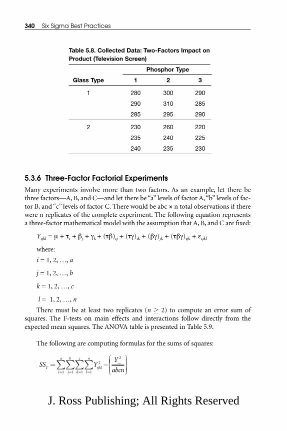
5.3.6 Three-Factor Factorial ExperimentsMany experiments involve more than two factors. As an example, let there bethree factors—A, B, and C—and let there be “a” levels of factor A, “b” levels of fac-tor B, and “c” levels of factor C. There would be abc × n total observations if therewere n replicates of the complete experiment. The following equation representsa three-factor mathematical model with the assumption that A, B, and C are fixed:
Yijkl = μ + τi + βj + γk + (τβ)ij + (τγ)ik + (βγ)jk + (τβγ)ijk + εijkl
where:
i = 1, 2, …, a
j = 1, 2, …, b
k = 1, 2, …, c
l = 1, 2, …, n
There must be at least two replicates (n ≥ 2) to compute an error sum ofsquares. The F-tests on main effects and interactions follow directly from theexpected mean squares. The ANOVA table is presented in Table 5.9.
The following are computing formulas for the sums of squares:
SS YY
abcnT ijkll
n
k
c
j
b
i
a
= −⎛
⎝====∑∑∑∑ 2
1111
2....⎜⎜⎜⎜⎜
⎞
⎠⎟⎟⎟⎟⎟
340 Six Sigma Best Practices
Table 5.8. Collected Data: Two-Factors Impact onProduct (Television Screen)
Phosphor Type
Glass Type 1 2 3
1 280 300 290
290 310 285
285 295 290
2 230 260 220
235 240 225
240 235 230
J. Ross Publishing; All Rights Reserved

= SSsubtotals(AB) – SSA – SSB
= SSsubtotals(AC) – SSA – SSC
= SSsubtotals(BC) – SSB – SSC
= SSsubtotals(ABC) – SSA – SSB – SSC – SSAB – SSAC – SSBC
The error sum of squares may be found by subtracting the sum of squares foreach main effect and the interaction from the total sum of squares, which couldbe presented as:
SSE = SST – SSsubtotals(ABC)
Obviously, factorial experiments with three or more factors are complicatedand will require several runs, particularly if some of the factors have several levels(e.g., more than two). Therefore, using a certain class of factorial designs (2k) iscommon if all factors are at only two levels. These designs are extremely easy toset up and analyze. Example 5.5 demonstrates how to utilize this model.(Subsection 5.3.7 will explain 2k Factorial Design.)
SSY
abcn
Y
abcnABC
ijk
k
c
j
b
i
a
= − −===
∑∑∑ . ....
2
111
2
SSS SS SS SS SS SSA B C AB AC BC− − − − −
SSY
an
Y
abcnSS SSBC
jk
k
c
j
b
B C= − − −==
∑∑ . . ....
2
11
2
SSY
bn
Y
abcnSS SSAC
i k
k
c
i
a
B C= − − −==
∑∑ . . ....2
11
2
SSY
cn
Y
abcnSS SSAB
ij
j
b
i
a
A B= − − −==
∑∑ .. ....
2
11
2
SSY
abn
Y
abcnCk
k
c
= −=
∑ .. . ....2
1
2
SSY
acn
Y
abcnB
j
j
b
= −=
∑ . .. ....
2
1
2
SSY
bcn
Y
abcnAi
i
a
= −=
∑ ... ....2
1
2
Improve 341
J. Ross Publishing; All Rights Reserved

Example 5.5: Analyze the Level of Significance of Three Factors
A processing engineer is studying the surface finish of a component that is pro-duced in a turning department. Three key factors affect the surface finish of thecomponent—tool feed rate (A), depth of cut (B), and tool angle (C). All three fac-tors have been assigned two levels and two replicates of a factorial design to col-lect the data for the experiment setup. Surface finish data are presented in codedform in Table 5.10A. In-process data are presented in Table 5.10B. Analyze thedata and state at which level of significance these factors are significant.
To test the data, set the null hypotheses:
H0: τi = 0 (no tool feed rate effect)
H0: βj = 0 (no depth of cut effect)
342 Six Sigma Best Practices
Table 5.9. ANOVA Table for a Three-Factor Fixed-Effect Model
Source of Sum of Degrees of Mean ExpectedVariation Squares Freedom Square Mean Squares F0
A SSA (a – 1) MSA F0 = MSA/MSE
B SSB (b – 1) MSB F0 = MSB/MSE
C SSC (c – 1) MSC F0 = MSC/MSE
AB SSAB (a – 1)(b – 1) MSAB F0 = MSAB/MSE
AC SSAC (a – 1)(c – 1) MSAC F0 = MSAC/MSE
BC SSBC (b – 1)(c – 1) MSBC F0 = MSBC/MSE
ABC SSABC (a – 1)(b – 1)(c – 1) MSABC F0 = MSABC/MSE
Error SSE abc(n – 1) MSE σ2
Total SST abcn – 1
στ
2
2
1+
−∑bcn
ai
σβ
2
2
1+
−∑acn
bj
σγ
2
2
1+
−∑abn
ck
στβ
2
2
1 1+
( )− −
∑∑cn
a bij
( )( )
στγ
2
2
1 1+
( )− −∑∑bn
a cik
( )( )
σβγ
2
2
1 1+
( )− −
∑∑an
b cjk
( )( )
στβγ
2
2
1 1 1+
( )− − −
∑∑∑n
a b cijk
( )( )( )
J. Ross Publishing; All Rights Reserved

H0: γk = 0 (no tool angle effect)
H0: (τβ)ij = 0 (no interaction effect of tool feed rate and depth of cut)
H0: (τγ)ik = 0 (no interaction effect of tool feed rate and tool angle)
H0: (βγ)jk = 0 (no interaction effect of depth of cut and tool angle)
H0: (τβγ)ijk = 0 (no interaction effect of all three factors—tool feed rate,depth of cut, and tool angle)
The following analysis shows the relation of the data with the model. (Thisanalysis can easily be done using MINITAB software.)
= 1998 – ((176)2/16) = 62
= ((79)2 + (97)2/8) – ((176)2/16) = 20.25
= ((82)2 + (94)2/8) – ((176)2/16) = 9
= ((83)2 + (93)2)/8) – ((176)2/16) = 6.25
= (((40)2 + (39)2 + (42)2 + (55)2)/4) – ((176)2/16) – 20.25 – 9 = 12.25
= (((37)2 + (42)2 + (46)2 + (51)2)/4) – ((176)2/16) – 20.25 – 6.25 = 0
= (((38)2 + (44)2 + (45)2 + (49)2)/4) – ((176)2/16) – 9 – 6.25 = 0.25
SSY
an
Y
abcnSS SSBC
jk
k
c
j
b
B C= − − −==
∑∑ . . ....
2
11
2
SSY
bn
Y
abcnSS SSAC
i k
k
c
i
a
A C= − − −==
∑∑ . . ....2
11
2
SSY
cn
Y
abcnSS SSAB
ij
j
b
i
a
A B= − − −==
∑∑ .. ....
2
11
2
SSY
abn
Y
abcnCk
k
c
= −=
∑ .. . ....2
1
2
SSY
acn
Y
abcnB
j
j
b
= −=
∑ . .. ....
2
1
2
SSY
bcn
Y
abcnAi
i
a
= −=
∑ ... ....2
1
2
SS YY
abcnT ijkll
n
k
c
j
b
i
a
= −⎛
⎝====∑∑∑∑ 2
1111
2....⎜⎜⎜⎜⎜
⎞
⎠⎟⎟⎟⎟⎟
Improve 343
J. Ross Publishing; All Rights Reserved

= (((18)2 + (22)2 + (19)2 + (20)2 + (20)2 + (22)2 + (26)2 + (29)2)/2) –((176)2/16) – 20.25 – 9 – 6.25 – 12.25 – 0 – 0.25
= 1.0
SSE = SST – SSsubtotals(ABC)
= 62 – 49 = 13
An ANOVA table is presented in Table 5.11. The following factors are signif-icant in Table 5.11: aTool Feed Rate (A) is significant at 1%; bDepth of Cut (B) andthe interaction of Tool Feed Rate and Depth of Cut (AB) are significant at 5%; andcTool Angle (C) is significant at 10%.
5.3.7 2k Factorial DesignThe 2k factorial design is very useful if each factor is at two levels. Because eachcomplete replicate of the design has 2k runs or treatment combinations, thearrangement is known as 2k factorial design. 2k factorial designs have a greatlysimplified statistical analysis. 2k designs also form the basis of many other usefuldesigns. The logic of two- and three-factors design will now be described.
5.3.7.1 22 Design
The simplest type of 2k design is the 22. If there are two factors, e.g., A and B, andeach factor is at two levels, generally these levels are assumed as low and high ofthe factor. A graphical design of 22 factorial is shown in Figure 5.7. The 22 = 4 runsform the corners of the square. Two types of notations are used in combinations:
• Treatment Combination—This combination is represented by lower-case letters. If the letter is present, then the corresponding factor is runat its high level in that treatment combination; if the letter is absent,the factor is run at its low level. For example, treatment combinationa indicates that factor A is at the high level. A treatment combinationwith both factors at the low level is represented by (1).
• Factorial Effect—The coefficients of factorial effects are always either+1 or –1.
The effects of interest in the 22 design are the main effects A and B and thetwo-factor interaction AB. The letters (alphanumeric) (1), a, b, and ab also repre-sent the total of all n observations taken at these design points. The main effect of:
SSY
abcn
Y
abcnABC
ijk
k
c
j
b
i
a
= − −===
∑∑∑ . ....
2
111
2
SSS SS SS SS SS SSA B C AB AC BC− − − − −
344 Six Sigma Best Practices
J. Ross Publishing; All Rights Reserved

• A = (Average observations on the right side) – (Average observations on the left side)
= ((a +ab)/2n) – ((b + (1))/2n)
= (1/2n) [a + ab – b – (1)]
Similarly, the main effect of
• B = (1/2n) [b + ab – a – (1)]
and
• AB = (1/2n) [ab + (1) – a – b]
Improve 345
Table 5.10A. Coded Surface Roughness Data for Example 5.5
Depth of Cut (B)
0.020 in. 0.035 in.Tool Angle (C) Tool Angle (C)
Tool Feed Rate (A) 12° 22° 12° 22° Yi…
15 in./min 10 12 9 118 10 10 9 79
Subtotal 18 22 19 20
25 in./min 9 10 12 1511 12 14 14 97
Subtotal 20 22 26 29
B � C Totals Y.jk. 38 44 45 49 Y…. = 176
Table 5.10B. In-Process Coded Surface Roughness Data for Example 5.5
A � B Totals A � C TotalsYij.. Yi.k.
B C
A 0.020 0.035 A 12 22
15 40 39 15 37 42
25 42 55 25 46 51
Y.j.. 82 94 Y..k. 83 93
J. Ross Publishing; All Rights Reserved

The quantities in brackets are known as contrasts, e.g., the A contrast is
ContrastA = a + ab – b – (1)
Table 5.12 can be used to determine the sign (plus or minus) for each treat-ment combination for a particular contrast. The column headings are the maineffects A and B and AB interaction, with I representing the total. The row head-ings refer to the treatment combinations. Important: The sign in the AB columnis the product of the signs from columns A and B. The sum of squares for A, B,and AB can be obtained as follows:
SS = (contrast)2/(nΣ(contrast coefficients)2)
Therefore,
SSA = [a + ab – b – (1)]2/4n
SSB = [b + ab – a – (1)]2/4n
SSAB = [ab + (1) – a – b]2/4n
The ANOVA is completed as usual with SST degrees of freedom (4n – 1) andSSE degrees of freedom 4(n – 1).
346 Six Sigma Best Practices
Table 5.11. ANOVA for Example 5.5
Source Sum of Degrees of MeanVariation Squares Freedom Square Fo Ftable
Tool Feed Rate (A) 20.25 1 20.25 12.462a F0.01,1,8 = 11.26
Depth of Cut (B) 9 1 9 5.538b F0.05,1,8 = 5.32
Tool Angle (C) 6.25 1 6.25 3.486c F0.10,1,8 = 3.46
AB 12.25 1 12.25 7.538b F0.05,1,8 = 5.32
AC 0 1 0 0
BC 0.25 1 0.25 0.154
ABC 1.00 1 1.00 0.615
Error 13.00 8 1.625
Total 60.0 15
aTool feed rate (A) is significant at 1%; bdepth of cut (B) and interaction of tool feedrate and depth of cut (AB) are significant at 5%; ctool angle (C) is significant at10%.
J. Ross Publishing; All Rights Reserved
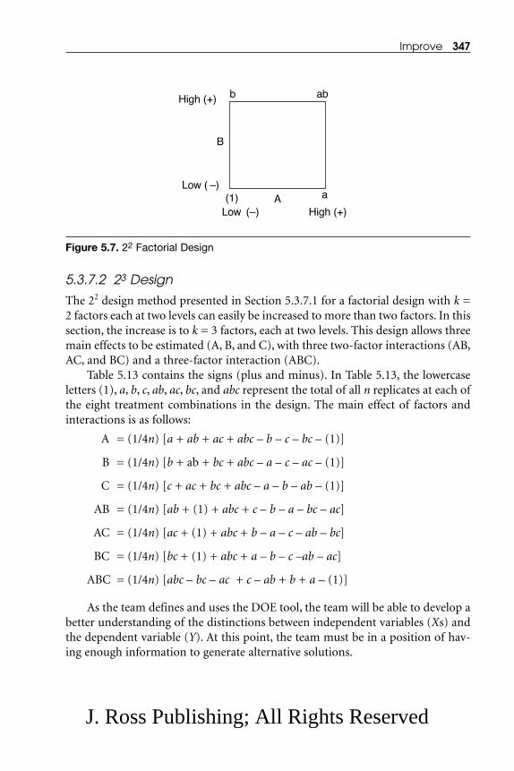
5.3.7.2 23 Design
The 22 design method presented in Section 5.3.7.1 for a factorial design with k =2 factors each at two levels can easily be increased to more than two factors. In thissection, the increase is to k = 3 factors, each at two levels. This design allows threemain effects to be estimated (A, B, and C), with three two-factor interactions (AB,AC, and BC) and a three-factor interaction (ABC).
Table 5.13 contains the signs (plus and minus). In Table 5.13, the lowercaseletters (1), a, b, c, ab, ac, bc, and abc represent the total of all n replicates at each ofthe eight treatment combinations in the design. The main effect of factors andinteractions is as follows:
A = (1/4n) [a + ab + ac + abc – b – c – bc – (1)]
B = (1/4n) [b + ab + bc + abc – a – c – ac – (1)]
C = (1/4n) [c + ac + bc + abc – a – b – ab – (1)]
AB = (1/4n) [ab + (1) + abc + c – b – a – bc – ac]
AC = (1/4n) [ac + (1) + abc + b – a – c – ab – bc]
BC = (1/4n) [bc + (1) + abc + a – b – c –ab – ac]
ABC = (1/4n) [abc – bc – ac + c – ab + b + a – (1)]
As the team defines and uses the DOE tool, the team will be able to develop abetter understanding of the distinctions between independent variables (Xs) andthe dependent variable (Y). At this point, the team must be in a position of hav-ing enough information to generate alternative solutions.
Improve 347
High (+)
Low ( –)
b
B
(1)Low (–)
AHigh (+)
a
ab
Figure 5.7. 22 Factorial Design
J. Ross Publishing; All Rights Reserved

Exercise 5.4: Analyzing Revenue and Factors that Impact SalesRevenue
A sales organization is analyzing its revenue data. The factors impacting its salesrevenue are presented in Table 5.14A. As a hired consultant, based on the infor-mation provided in Tables 5.14B and 5.14C, provide recommendations.
5.4 SOLUTION ALTERNATIVES
As a Six Sigma team progresses through the analyzing phase of a project in whichthe team must identify objectives and alternative solutions for theproduct/process to achieve the defined goals/objectives, the entire improvementprocess may be summarized into three stages:
348 Six Sigma Best Practices
Table 5.12. Signs for Effects in 22 Design
Treatment Factorial Effect
Combination I A B AB
(1) + – – +
a + + – –
b + – + –
ab + + + +
Table 5.13. Signs for Effects in 23 Design
Treatment Factorial Effect
Combination I A B AB C AC BC ABC
(1) + – – + – + + –
a + + – – – – + +
b + – + – – + – +
ab + + + + – – – –
c + – – + + – – +
ac + + – – + + – –
bc + – + – + – + –
abc + + + + + + + +
J. Ross Publishing; All Rights Reserved

Improve 349
Table 5.14A. Factors Impacting Sales Revenue
Level
Factor Low High
Sales Representative’s Participation No YesSales Representative’s Experience ≤1 year >5 yearsExisting or New Customer Existing NewAdvertising No YesSales Promotion No Yes
Table 5.14B. Sales Information for Scenario 1
Scenario 1:
(A) X1: Sales Representative’s Participation(B) X2: Existing or New Customer(C) X3: Advertising
X1 X2 X3 Y1 Y2
– – – 15 14+ – – 25 26_ + – 27 28+ + – 28 30– – + 20 19+ – + 22 23– + + 17 16+ + + 29 30
Table 5.14C. Sales Information for Scenario 2
Scenario 2:
(A) X1: Sales Representative’s Experience(B) X2: Existing or New Customer(C) X3: Sales Promotion
X1 X2 X3 Y1 Y2
– – – 15 15+ – – 25 26– + – 24 25+ + – 27 28– – + 20 19+ – + 29 30– + + 24 25+ + + 28 29
J. Ross Publishing; All Rights Reserved

• Investigate
• Evaluate and Propose
• Implement
Key elements of these stages are presented in Table 5.15.
Another way of looking at the improvement process is to ask, “What con-stitues the bottom line of a Six Sigma project?” Some answers might include:
• To Generate Alternate Solutions—Team will need to either analyzethe historical data or first collect the data and then analyze it (or acombination of both) to develop the alternative solutions. In theprocess, the team will need to identify constraints. The team might be
350 Six Sigma Best Practices
Table 5.15. Summarized Process Stages
Investigate Should Lead to
DevelopingAlternative Solutions Evaluate and Propose Implement
• Process Mapping
• Brainstorming
• Creative Thinking
• CTQs
• Cause-and-EffectDiagram
• FMEA
• Benchmarking
• Process/Product CostAnalysis
• Problem Solving Process
• Information Collection:Qualitative and/orQuantitative
• Graphing Tools
• Analyzing Tools:Hypothesis Testing–Classical, Chi-Square,ANOVA, Regression, and Correlation
• Criteria-Based Decision Matrix
• Develop Alternatives
• Cost/Benefit Analysis
• Risk Analysis
• Pilot Testing Alternatives
• Cost/Benefit Analysis
• Propose Best Alternative
• Resource Training
• Resource Upgrading
• Schedule/WorkBreakdown Structure
• Control Plan
• Implementation
J. Ross Publishing; All Rights Reserved

able to benchmark similar processes and eliminate unrealistic orinfeasible alternatives.
• To Assess Risk—The team will need to assess risk as it relates to alter-native solutions and their impact on customers, the business, employ-ees, federal, state, and local regulations, and the bottom line of thebusiness.
• To Perform an Initial Study to Test Alternatives—An initial study maybe accomplished using a small-scale experiment or by using pilotprojects.
• To Evaluate and Select the Best Alternative to Meet/Exceed theDefined Objectives—As the team is solving a problem, it is importantfor team members to understand how their processes have evolved tothe current state and to try to utilize this information to develop acomprehensive solution to the problem. This might require testingseveral alternatives. Because different tools are used in individualbusinesses for identifying, evaluating, and selecting alternative solu-tions, the team should check the type of tools used in its business. Ifthe team feels comfortable with these tools, the team can utilize them.As the team goes through the improvement process, it is critical thatit remains focused on the critical input variables (Xs) as identified inthe Analyze phase.
5.5 OVERVIEW OF TOPICS
This section will provide a brief overview of topics that have been discussed inprevious chapters.
InvestigateThe investigation concept is described in detail in Chapters 1, 2, and 3. Selectedtopics are now briefly discussed.
Process Mapping—Process mapping is generally utilized for:
• Developing and understanding a process/workflow
• Identifying alternative processes
• Eliminating redundancies, loops, waste and non-value-added activi-ties, and delays
• Consolidating activities to streamline the process
• Facilitating resources planning
Improve 351
J. Ross Publishing; All Rights Reserved

Process mapping should be developed by actual users as well as Six Sigmateam members. These mappings should be analyzed. Then a real (or actual)process map should be developed. An actual process map should lead to animproved process map.
Brainstorming—One of the easiest ways to generate a high volume of ideasis by using brainstorming sessions. Concepts could be applied to generate alterna-tives. Mathematical/statistical tools are also a source of generating alternatives.They may be used to test the alternatives developed from brainstorming. Rulescommonly followed during brainstorming session include:
• Make no judgment, analysis, or criticism of the ideas.
• Capture all ideas.
• Build on the ideas and creativity of others.
• Encourage participation by all team members.
• Limit the session. Keep the time frame short (typically 15 to 25 min-utes).
Creative Thinking—The key to creative thinking is that “rules and regula-tions” should not stop anyone from asking questions. The team should ask ques-tions about each element/activity of the process/product. Think about severalquestions while keeping the customer’s needs and expectations in mind:
• Why has the activity been performed? Can it be eliminated?
• Who performs the activity? Can someone else perform it?
• Where has the work been done? Can it be done somewhere else?
• What resources are required? Where else could resources be found?
• Under what conditions is work done? Can those conditions bechanged?
• What is the value added by the work? Can it be improved?
Key thought-generating questions include:
• Why? � Substitute/Eliminate?
• Who? � Sources to Substitute?
• How? � Process Change/Modify/Eliminate?
• When? � Present/Future?
• What? � Optional/Required/Eliminate?
352 Six Sigma Best Practices
J. Ross Publishing; All Rights Reserved

CTQs—The product or process performance characteristics must satisfy cus-tomers. Therefore, it is important to define CTQs (critical to quality characteris-tics) for customers. Defining customer CTQs, requires a three-step process:Identify � Research � Translate. This process delivers:
• Prioritized internal and external customer lists; also identifies stake-holders
• Prioritized customer needs
• CTQs to support customer needs
Ensure that all information (company and customer) is in the same language.Then compare team research output with the customers’ suggested needs andwants and prepare a gap analysis. This gap analysis will lead to CTQs. Simpleguidelines to translate customer requirements into needs and wants include:
• State customer needs and wants.
• Have measurable terms in CTQs.
• Reflect a positive attitude in written text.
• Confirm or verify needs and wants with customers.
• Write simply and in complete sentences. Ensure specific issues areaddressed.
Cause-and-Effect Diagram—A cause-and-effect diagram is an analysis toolthat provides a systematic way to look at effects and the causes that create or con-tribute to those effects. Cause-and-effect listings are also useful to summarizeknowledge about the process. A cause-and-effect diagram is designed to assist ateam in categorizing all (sometimes many) potential causes of problems or issuesin an orderly way and identifying root causes.
FMEA—FMEA is an iterative process. It is used for system design, manufac-turing, maintenance, and failure detection. Key functions include:
• Identifying unacceptable effects that prevent achieving designrequirements
• Assessing the safety of system components
• Identifying design modifications and corrective action needed to mit-igate the effects of a failure on the system
FMEA helps to keep each responsible group focused on its responsibilities asthe product goes through its life cycle. In the FMEA process, the system is treatedas a “black box” with only its inputs and the corresponding outputs specified.
Improve 353
J. Ross Publishing; All Rights Reserved

Benchmarking—Benchmarking involves sharing process and business infor-mation about one company with other company. Most businesses have developedprocedures to manage and monitor the company’s involvement in benchmarkingvisits. Before planning a visit to any external business, consult business manage-ment at your company about these policies and procedures. A benchmarkingprocess will assist in:
• Measuring business performance or processes at a business againstthe best-in-class practices of other businesses
• Determining how other businesses achieve their performance levels
• Providing information to improve one’s own performance
Process/Product Cost Analysis—Every business has its own methods to ana-lyze process/product costs that should be followed. Follow the company’s already-developed costing guidelines. Basic rules in a costing process can include:
• Keeping cost data as realistic as possible
• Utilizing the same logic for the present process/product as well as forthe developed alternatives without adding any unrealistic cost factors,e.g., a cost element in overhead applies to one very specificprocess/product, but this cost element is distributed over allprocesses/products
• Comparing all cost data (present process/product and alternatives) inpresent dollars and before taxes (federal and state)
Problem-Solving Process—In many situations, a problem-solving process isdesigned to find a simpler or faster procedure that will result in an improvement.During a problem-solving process, listening to and acting upon the suggestions ofemployees who are closely involved with the process/product is important. Theseemployees could provide information that would help the team to make a deci-sion quickly. Commonly used steps in the problem solving process include:
• Identifying the problem area and defining the problem (issue)
• Collecting background data and designing focused questions (Applythe concepts presented in Chapters 2, 3, and 4—Define, Measure, andAnalyze. Develop questions starting with “what” and “how.” “What”questions are used to identify process/product elements. “Why” ques-tions are used to solve the issue/problem.)
• Identifying employees who should participate in the discussion(Diversity in the team is critical to get new ideas. Team size should belimited to no more than 12 members.)
354 Six Sigma Best Practices
J. Ross Publishing; All Rights Reserved

• Identifying a meeting facilitator so that he/she may do his/her “home-work” before the meeting
• Conducting a problem-solving session and providing team memberswith all necessary information 1 week before the session
• Identifying and obtaining (reserving) all supportive material so that itis available at the time of the meting
• Communicating problem-solving recommendations to all interestedparties and implementing the recommendation according to a devel-oped schedule
• Recognizing the problem solving team for its achievements
Evaluate and ProposeOnce process/product issues have been identified, the next steps are collectinginformation, utilizing presenting tools to present the collected information, andutilizing analyzing tools to analyze the collected information. Detailed supportivematerial about these topics may be found in Chapters 3, 4, and 5. Selected topicsare now briefly discussed.
Risk Analysis—Before conducting any pilot testing, evaluate the risks (safetyand security) associated with each alternative in relationhip to:
• Customers—Impact in relationship to current exposure: alternativesmust provide better safety and security.
• Employees—Safety and security issues are similar to customers.
• Compliance—Depending on the location (usage) of the product/service, compliance must satisfy local and global safety and securityrequirements.
• Business Goals—Selected alternatives should be in line with businessgoals/objectives.
Evaluate risk associated with any alternative by:
• Identifying risks, e.g., safety, security, market share, technical quality, etc.
• Analyzing the risks
• Planning, communicating, and obtaining business/complianceauthority approval before testing pilot alternatives
• Tracking and maintaining risk data
A team should evaluate risk at several stages of a DMAIC process. At thispoint, only testing risk(s) are to be evaluated/questioned. Risk analysis will be
Improve 355
J. Ross Publishing; All Rights Reserved

required again when the selected alternative is implemented to improve theprocess/product.
The Simulation Tool—Simulation is a powerful analyzing tool. Importantcharacteristics of the tool include:
• Simulation can be used with a detailed process model to determinehow the process output (Y) would respond to changes in the processstructure, inputs (Xs), and/or neighboring independent variables(Xs).
• Simulation can be used to test alternative solutions. The simulationevents can be discrete or continuous:
– Discrete Events Simulation—Discrete events occur at distinctpoints in time. These events control process performance.
– Continuous Simulation—A simulation utilized if process param-eters change continuously.
• Simulation can be used:
– To identify intricate and specific issues in the existing or proposedprocess
– To develop a model realistically close to the real situation/process
– To predict the behavior of the process under varying conditions(constraints)
• Simulation can help the team to generate process data that might beneeded to make decisions about the design and the operations of theprocess.
• Simulation might not solve a specific problem, but it can help theteam to identify problems and evaluate alternative solutions throughquantitative information under a variety of conditions.
• A simulation model is “virtual reality.” Different process situationswill need different types of simulation.
Simulation model development is the most time-consuming activity in thesimulation process. If the model developed is not a fairly accurate representationof reality, the model will be of no benefit. Remember: “Garbage in, garbage out.”Model steps may be linear, simultaneous, or iterative. A sample linear model ispresented in Figure 5.8.
Pilot-Testing Alternatives—Pilot testing involves testing, at a small scale, ofall or part of a proposed solution to better understand the proposed solution andto learn how to achieve a more-effective full-scale implementation. Pilot testingcan be in the following categories:
356 Six Sigma Best Practices
J. Ross Publishing; All Rights Reserved

• To test the complete solution
• To test isolated elements of a solution and/or isolated locations
• To test for robustness
Several activities generally support pilot testing and a successful program:
• Communicating periodically with business leadership to obtain lead-ership’s full support
• Developing a detailed plan for pilot testing
• Selling the pilot plan to all associated employees who will be affectedby it
• Training associated employees
• Monitoring pilot implementation
Improve 357
Figure 5.8. Flow Chart: Simple Linear Simulation Model
ProcessSpecification
Identify Variablesand Constraints
Develop Model
Test and ValidateModel
ModelSensitivityAnalysis
Analyze SimulationModel Output?
ModelDoes
Not MeetObjectives
Model MeetsObjectives
ModifyModel
Plan of ModelImplementation
Implement theModel
MonitorPerformance
CompleteDocumentation
Utilize Output(s)in Planned Area(s)
Start
Complete
J. Ross Publishing; All Rights Reserved
• Analyzing pilot information utilizing proper statistics
• Designing a closed-loop system to improve/adjust the proposed solu-tion
• Assessing execution of the pilot
Cost/Benefit Analysis—Key elements of a cost/benefit analysis include:
• Buy-In—As other employees (not members of the team, e.g., finan-cial, sales, design, service) participate in cost/benefit analysis andaccept the data, their buy-in and support for the project will be gen-erated.
• Communication—A formal cost/benefit analysis should be commu-nicated in financial terms. Describe the project to the financial groupand other interested parties so that they can evaluate it the projectmakes good business “sense” or if it does not.
• Calculations—A cost/benefit analysis may include calculations suchas net present value, cashflow, internal rate of return, return on equity,payback period, and other financial information of interest.
• Refined Data—Cost/benefit data at this stage of a project should berefined when compared to the estimated data that was available whenthe project statement was developed.
The importance of a cost/benefit analysis is to identify all benefits—tangible,intangible, and/or both. Identifying all benefits is essential. A cost/benefit analysisallows determination of whether or not a project has a clear financial payback.Benefits should be aligned with the business metrics and should be trackedaccordingly. Experience has shown that teams generally underestimate the impactof their projects. Utilize the financial department at the business to ensure that alldata concerning all benefits realized from this project have been collected.
Guidelines for a cost/benefit analysis typically involve a simple process,although an individual business/workplace may require additional information tomeet its requirements:
• Estimate benefits to be gained
• Estimate implementation and operating costs for the improved prod-uct/process
• Determine net financial improvements
• Identify intangible benefits
Therefore,
358 Six Sigma Best Practices
J. Ross Publishing; All Rights Reserved

Total improvement = Net financial benefits + Intangible benefits
= (Tangible benefits – Implementation costs) + Intangible benefits
The team should prepare a cost/benefit analysis with the help of the financialdepartment. Guidelines include:
• Direct Savings/Benefits—Determine the impact and appropriatemeasurements for the activities/process/product. Use standard oraverage rates as they apply in the business and obtain savings/benefitsdata.
• Financial Benefits—Financial benefits from a project are possible onlyafter successful implementation of the team’s recommended improve-ments. Therefore, subtract implementation costs from tangible bene-fits or financial gains as projected (estimated) above. Even ifintangible benefits are not measureable for financial purposes, intan-gible benefits are generally considered to be favorable outcomes thatjustify the value of the project.
• Prepare a Formal Financial Cost/Benefit Analysis—A formal financialcost/benefit should be prepared for the selected solution. It shouldupdate the financial opportunity derived from the project, which wasestimated in the Define phase and refined in the Analyze phase. Theformal final financial analysis must include intangible benefitsderived from the project.
A simple pay-off matrix is shown in Table 5.16. A pay-off matrix will help theteam to evaluate the alternative solutions in relationship to the efforts requiredand the benefits anticipated. Important: All the team members should share thesame operational definitions of high and low.
Implement The next step is to implement the selected alternative to meet project objectives.Before implementing the selected alternative, examine:
• Resources Training—Review understanding of the process to beimplemented with all affected employees. Answer their questions andeliminate their concerns. Analyze the employee knowledge base todetermine if any training is needed before implementing the recom-mended solution.
• Resource Upgrading—Resources other than employees include facil-ity, equipment, technology, etc. Review these resources, e.g., addresssafety issues. Equipment and/or the facility may need to be upgradedto meet local, state, and federal safety requirements.
Improve 359
J. Ross Publishing; All Rights Reserved

• Schedule and Work Breakdown Structure—As the workforce under-goes training, employees must also have training for the improvedprocess so they understand the process structure. Process break-down/structure is generally a good tool for training and a referencepoint for the process owners. An implementation schedule is also agood management tool. Project implementation should be trackedagainst the developed schedule.
• Control Plan—Relating gains achieved from a Six Sigma project isimportant. (Several elements that help to retain the gains will be dis-cussed in detail in Chapter 6, Control.)
During project implementation, the team must monitor project progress andalso listen to comments and concerns of participating employees. If the imple-mentation plan progresses smoothly, the project team and other participatingemployees will see the improvements. It is critical to monitor the implementationschedule, process improvements, financial benefits, and input from participatingemployees. The financial benefits of implementing Six Sigma projects are gener-ally very attractive—increased revenue, improved business margin, reduced cycletime, and higher inventory turns. A cost/benefit exercise is presented in Exercise 5.5.
Exercise 5.5: Analyzing Costs vs. Benefits
The XYZ division of a corporation produces an electromechanical, software-con-trolled product. The XYZ division does not manufacture any components.Outside suppliers and sister divisions of XYZ supply the components. The XYZproduct is an integrated and tested system that is made up of three modules: A, B,and C. These three modules (A, B, and C) are assembled and tested at XYZ divi-sion. The total manufacturing process at XYZ division is presented in Figure 5.9.Material costs are as follows:
360 Six Sigma Best Practices
Table 5.16. Pay-Off Matrix
Accepted Alternative Rescope/ReconsiderHigh for Continuation Alternative
Benefits
Reject Alternative Reject AlternativeLow
Low High
Effort
J. Ross Publishing; All Rights Reserved

Module A = $15K per unit
Module B = $3K per unit
Module C = $2K per unit
The Six Sigma team has investigated and analyzed historical data for the totalmanufacturing cycle and has found two critical issues with highest priority:
• Technical support in the module assembly and test areas is not avail-able when needed due to poor scheduling.
• Parts shortages exist on the manufacturing floor because suppliers aremissing delivery dates.
Improvement has been proposed by the team:
• Modify the current supplier contract from 6 months to 2 years. Thiswill guarantee quality on-time parts delivery with a 1% reduction inmaterial cost. Because workers will not have to wait for parts, esti-mates are that the assembly and test work will be reduced by 15%.
• Purchase and install scheduling software to improve the chances oftechnical resource availability in the module assembly and test areas.The scheduling software will cost $20K. Installation and training costswould be $5K.
Once the above-listed improvements are implemented, the team has esti-mated that the manufacturing cycle time for assembly and test areas will bereduced by 25%.
Additional information includes:
• Wage rate for assembly and test workers—$5/hour
• Benefit cost for assembly and test workers—25% of wage rate
Improve 361
ModuleAssemblyand Test
ActualWork Time
(Hours)
SystemIntegration and
Test Time(Hours)
Covering andPackaging
Time(Hours)
A 8 B 6 16 8 C 5
Average Manufacturing Cycle in Calendar Days
Readyto
Ship
10 5 217
Figure 5.9. Total Manufacturing Process for a Product at XYZ Division of aCorporation
J. Ross Publishing; All Rights Reserved
• Annual inventory carrying cost—12%
• Total manufacturing overhead—300% percent of workers’ wage rates
• Annual capital borrowing cost—8%
• Annual inflation adjustment rate—3%
• Annual production forecast—180 systems
Develop a cost/benefit analysis and state assumptions.
Conceptual SummaryDiscussion so far has been about the process from project proposal through toimplementation of the recommended solution. As the Six Sigma team worked onthe project from the Define phase through the implementation of the recom-mended solution to achieve the stated project goals, the team needs to considerseveral questions:
• How does the solution address the root cause(s) of the problem?
• How did the team generate alternative solutions?
• What criterium(a) did the team use to evaluate potential solutions?
• What did the team develop as a “should be” process map (incorporat-ing changes in the process)?
• How would the team manage cultural aspects required for successfulchange. Has the team mobilized support?
• What level of risk assessment was done before the pilot/small-scaleproject test?
• Was the solution tested as a pilot process or on a small scale? What waslearned from the test?
• If the solution has many components, did the team test some isolatedelements? As an example, if the team’s solution is to implement acompany-wide communication network, a few elements of the systemcan be selected from different sections of the business to evaluate per-formance, which would help the team to determine whether or notthere will be any conflicts with the existing network.
• How robust is the proposed system or process? What happens whenthe system is overloaded with inputs or unexpected events? Whatinstructions are provided to users? How well does the alternative solu-tion perform under adverse conditions? As an example, if the teamwere testing a call center in the communication network, and theycould load the network with an excessive number of calls to deter-mine whether or not some new bottlenecks had been created, how
362 Six Sigma Best Practices
J. Ross Publishing; All Rights Reserved

could the excessive load be relieved? Examining robustness could cre-ate a next level of issues that need to be addressed/resolved.
• What are potential problems? Does the team have a backup plan if“things go wrong?”
• What is the implementation plan? How would the team knowwhether or not the plan has been followed?
• Can team members explain their cost/benefit analysis includingassumptions the team made to others?
5.6 SUMMARY
In the first five chapters, four phases of the DMAIC process have been discussed—Define, Measure, Analyze, and Improve. This chapter has discussed the Improvephase. Improvement means “reducing variation or improving a process;” there-fore, process improvement solutions have been discussed. Starting with theimprovement strategy led to establishing a quantitative relationship between theindependent variables (Xs) and the dependent variable (Y). The tool used forrelationship establishment was DOE (the design of experiments). Several stepsdeveloped alternative solutions, selected the most appropriate solution tomeet/exceed the goals/objectives of the Six Sigma project, and then implementedthe selected process improvement. Topics discussed in this chapter include:
• Improvement Strategy
• Process Reengineering
• Guide to Improvement Strategies for Factors and Alternatives
• Introduction to Design of Experiments
– Completely Randomized Single-Factor Experiment
– The Random-Effect Model
– Factorial Experiments
– Design of Experiments Terminology
– Two-Factor Factorial Experiments
– Three-Factor Factorial Experiments
– 2k Factorial Design
• Solution Alternatives
– Investigate
– Evaluate and Propose
– Implement
• Conceptual Summary
Improve 363
J. Ross Publishing; All Rights Reserved

A project team should determine if the following steps were followed beforeproceeding to Control, the next phase of the DMAIC process:
• Generate and test possible alternatives so that a proper selection canbe made to meet/exceed the project goals/objectives. Key in-processelements that should have been followed include:
– Analysis and testing
– Development of process map
– Cost/benefit analysis
– Testing the improvement alternatives with small-scale/pilot solu-tion implementation
– Implementation of any process modification required based onthe pilot data and analysis
• Design the implementation plan. Then implement the selectedimprovement process. The implementation plan should includeworkforce training, resources upgrading, schedule/work breakdownstructure, and a control plan. Always have a contingency plan in caseimplementation does not go as planned.
• Monitor (a team responsibility):
– How possible alternative solutions have been developed
– Tools that have been used to tap into the creativity and encour-agement of participants
– Tools that have been used to select the best alternative
– The type of criteria the team has developed to test and evaluatepotential alternatives
– The assumptions that have been made in the cost/benefit analysis
– The basic guidelines that have been used in risk analysis
– If there were any constraints (technical, governmental, cultural,or other) that could have forced the team to reject certain alter-native solutions
– How the pilot test was run, the data were collected and analyzed,and conclusions were drawn
– The lessons learned, if any, from the pilot that have been incorpo-rated into the design of the full-scale solution
– How good the implementation plan has been
– How good the process map/design has been and any issues orconcerns
– How well the selected solution has eliminated/minimized keysources of variation
364 Six Sigma Best Practices
J. Ross Publishing; All Rights Reserved
– Tools that were most useful during the Improve phase of theDMAIC process
– Different elements of communication that were necessary to sup-port the implementation of the selected solution
– How process owner(s) have monitored the implementation planand recognized its intended improvements
– The team’s contingency plan to handle any potential problemsduring implementation
Once the project has been implemented and is performing as planned, thenext question that comes to mind is, “What kind of control measures are neededto ensure that the implemented solution stays successful? This question will beanswered in Chapter 6.
REFERENCES
1. Hammer, M. 1996. Beyond Reengineering. New York: Harper Collins.
2. Kumar, D. 2003. Lean Manufacturing Systems. Unpublished.
Improve 365
This book has free material available for download from theWeb Added Value™ resource center at www.jrosspub.com
J. Ross Publishing; All Rights Reserved

J. Ross Publishing; All Rights Reserved

6
CONTROL
A Six Sigma team’s responsibility does not end once a recommended solution hasbeen implemented. At this point, the project represents a “milestone” accomplish-ment, yet significant effort still will be required to take the project to completion.The team has the responsibility of leading/guiding several activities, which arecritical for project completion:
6.1 Self-Control
6.2 Monitor Constraints
6.3 Error Proofing
6.3.1 Employee Errors
6.3.2 The Basic Error-Proofing Concept
6.3.3 Error-Proofing Tools
367
Define
Measure
Analyze
Improve
Control
6σ DMAIC
J. Ross Publishing; All Rights Reserved

368 Six Sigma Best Practices
6.4 Statistical Process Control (SPC) Techniques
6.4.1 Causes of Variation in a Process
6.4.2 Impact of SPCs on Controlling Process Performance
6.4.3 Control Chart Development Methodology and Classification
6.4.4 Continuous Data Control Charts
6.4.5 Discrete Data Control Charts
6.4.6 SPC Summary
6.5 Final Project Summary
6.5.1 Project Documentation
6.5.2 Implemented Process Instructions
6.5.3 Implemented Process Training
6.5.4 Maintenance Training
6.5.5 Replication Opportunities
6.5.6 Project Closure Checklist
6.5.7 Future Projects
6.6 Summary
References
Retaining the gains made from a Six Sigma project is important. Concepts andideas that the team may need to follow/implement will now be presented. A com-bination of these ideas may be required to retain the improvements made.
6.1 SELF-CONTROL
Once a recommended solution has been implemented, the team must think aboutthe following questions:
• Is the implemented solution capable of meeting the expected projectgoals?
– Is the project holding Six Sigma metrics goals?
– Are data from the implementation solution validating theexpected relationship between the independent variables (Xs)and the dependent variable (Y)?
– Is the process stable and under control?
• Is the process not stable enough and still changing? If so, should theteam intervene or not?
J. Ross Publishing; All Rights Reserved

• Do employees (workers) have the necessary knowledge, experience,and tools? Are they capable of meeting expected performance levels?
• Do workers have the authority to make the required adjustmentswithout any major administrative “red tape?”
• Do workers understand their responsibilities and goals? Have theirtargets been clearly spelled out?
• Are any feedback mechanisms in place so that workers know how wellthey are doing in relationship to expectations?
If the answers to the above questions are generally “yes” or “positive,” thebusiness has been providing what is known as “self-control” or the optimal con-ditions for the process.
Self-control also implies that workers understand the basic elements of theirjobs and have been motivated to expend their efforts to change and improve theresults of their efforts. Therefore, the “bottom line” is that workers have becometheir own feedback loop. If employees are provided with responsibilities andauthority over their surroundings, they receive a higher status and a form of“ownership.”
Other important questions include:
• Do workers (who now “own” the process) have the resources and anawareness of documentation? As an example, several documents anddisplays should be accessible to workers. Workers should also knowhow to use these documents:
– Written process/product specifications
– Service conformity standards and work instructions
– Same document edition (or version) at all locations
– A display of defective products and services for educational pur-poses
– Policy and procedures about deviation from the standard
• Do workers have mechanisms in place to know about their perform-ance in relationship to standards?
– Feedback mechanisms
– Performance metrics
– Quality inspectors/examiners
• Do workers have the resources required to improve their performanceif they have been performing below the expected standard?
– Periodic measurement of product/process quality
– A guide to improve worker performance
Control 369
J. Ross Publishing; All Rights Reserved
Provide as much quality control to the operating workforce as possible. Thisprovides the shortest feedback loop. It also requires that the process implementedby system designers be capable of meeting product quality goals. Employeeempowerment, i.e., for the employees responsible for the process, is anotherimportant factor for designers to consider when designing controls in the system.Employee self-control means that workers understand the key elements of theirjobs and are motivated to expend their efforts to change and/or improve theresults of their efforts. The bottom line is that workers become their own feedbackcontrol (improvement) loop. Therefore, workers must understand their jobassignments and think that they are the part of the process/system, which resultsin a sense of “ownership” for employees.
Resources are constraints in any business/process. How resources are utilizedis key for any business to succeed in a globally competitive market.
Exercise 6.1: Self-Assessing a Process
• Select a work process you perform and briefly describe it.
• What is the expected result(s) of the process?
• What metrics do you use to measure the performance of yourprocess?
• What kind of feedback mechanism do you use to correct yourprocess?
• What level of self-control responsibility and authority do you have?
6.2 MONITOR CONSTRAINTS
Several constraints impact a process/product. The impact of all constraints is notequal. Generally recognized constraints include:
• Material • Metrics• Process • Information• Technology • Training• Workforce • Environment• Equipment • Utilities
Many businesses measure resource utilization and wait until the output isgenerated before action is taken, which is often too late. Controls should be placedwithin the process. To produce a better-quality product, controls must be put intoeffect well before the output is produced.
Deciding exactly which constraints to select can be difficult for the team. Theteam is well advised to identify the most critical constraints (or vital few) and give
370 Six Sigma Best Practices
J. Ross Publishing; All Rights Reserved

these constraints appropriate attention. Then, select one constraint that is moreimportant than all of the others. Once a constraint is selected, analyze the impactof the selected constraint on:
• The process
• The constraint’s performance
• The processed output
As an example, the constraint selected is “workforce.” The workforce isrequired to support the process. The workforce must be dynamic and must adjustaccording to process change. The workforce must also have the skills and experi-ence to support an ever-changing process. Worker training, feedback for errorcorrection, and job rotation are critical elements to maintain a high workforceperformance level.
As another example, select as the constraint “material,” which is one of the keyinput elements in an SIPOC process. The combination of input elements and in-process activities produces the output to meet customer needs. To have qualitymaterial for the process, material quality must be maintained at the supplier’sworkplace.
A Six Sigma team needs to answer key questions about monitoring:
• What should I (the team) monitor?
• Where should I (the team) monitor?
• How do I (the team) monitor?
• When do I (the team) monitor?
What Should I (the Team) Monitor?All monitoring should be centered on a specific resource that the team wants tomonitor. Monitoring does not work without a feedback loop. Resource monitor-ing is a combination of:
• Process features
• Product features
• Side effects of process and/or product features
Process Features—Most monitoring is utilized to evaluate process featuresthat most directly affect the product, e.g., coolant chemistry in a turning machineis utilized to keep tool temperature low enough to achieve the surface finish on apart; ink in an ink jet printer is used for printing addresses on envelopes; etc.Several process features become candidates for monitoring subjects as a means ofeliminating or minimizing failures. These monitoring elements are generallyselected based on historical data, FMEA analysis, and/or research data. These
Control 371
J. Ross Publishing; All Rights Reserved

process features-related monitors are linked to the decision question, “Should theprocess be run or stopped?”
Product Features—Some monitors are utilized by evaluating the product’sfeatures, e.g., copying paper must be at a certain minimal weight to be utilized ina copying machine. Therefore, the major activity is an inspection to check prod-uct specifications or objectives. This type of activity is generally performed atdefined product phases in which breakdowns may have occurred in the produc-tion process.
Side Effects of Process and/or Product Features—These features generally donot affect the product, but they may create side effects, e.g., certain activities in thebackyard of a house may be offensive to the neighborhood; chemical leaks from aplant may create threats to the environment; etc.
Where Should I (the Team) Monitor?Constraint review stations are usually designed to provide evaluations and/orearly warnings at several phases:
• Before starting on a significant, irreversible activity, e.g., a preflightcheck that astronaut goes through before mission control allows anastronaut team to take off for a space project mission
• At changes of responsibility and/or authority, a time at which eitherone or both are transferred from one organization to another
• After creation of a critical quality feature
• At the site of dominant process variables
• At areas that allow an economical/financial evaluation to be made
Generally, a flowchart of the process is very useful in identifying a group ofconstraints within appropriate monitoring stations. Key areas to set up monitorsinclude:
• At the start of a significant, irreversible activity
• When authority changes
• After creation of a critical quality feature
• At the site of dominant process variables
How Do I (the Team) Monitor?The feedback loop is a tool used to monitor the actual performance of aprocess/product and to keep it performing as designed (known as a closed-loopsystem). A feedback loop flow chart is presented in Figure 6.1.
372 Six Sigma Best Practices
J. Ross Publishing; All Rights Reserved

Components of a feedback loop (“sensor,” problem analysis) could be a com-bination of mechanical, electrical, software, and employees. Feedback loops are anintegral part of the process design and control system. They keep the process per-forming as designed, e.g., a thermostat, a fuel gauge in automobile, etc. The flowof information and activities within a feedback loop includes the following:
• Actual performance of the operating process is first measured.
• The results or outputs of the process are compared against an estab-lished standard or control target. The tool used to measure the processis usually referred to as the “sensor.”
• Based on the established objectives/guidelines, a decision is madeabout whether there is adequate conformity or not. The decision-maker is generally called a “judge” or “umpire.” If performance meetsor exceeds established guidelines, the process continues to run.
• If performance does not meet the target, the umpire begins analyzingto identify the problem, diagnose the causes, and to initiate a series ofactivities that will adjust the process and restore conformance.Performance is brought in line with the target. Operation of the feed-back loop continues as long as the process stays within the guidelines.
Control 373
MeasureActual
Performance
Compareto Standards
(Sensor)
Update/ModifyControl
Standards
IdentifyIssue
DiagnoseCause
InitiateCorrective
Action
Problem Analysis
OK
Not OK
Figure 6.1. Feedback Loop Flow Chart
J. Ross Publishing; All Rights Reserved

When Do I (the Team) Monitor?The timing of process monitoring is critical. It can take place at several stages as aprocess progresses. Commonly used stages include:
• At the start of a process
• During the process
• During supporting operations
At the Start of a Process—Results of a monitored process are used to decidewhether or not to start the process, e.g., preflight takeoff process checks.Generally, monitoring involves:
• Following preparatory steps to get ready for a process—Usually, theproduct/process supplier provides these steps.
• Evaluating the start monitoring information to determine whether, ifstarted, the process will meet the goals
• Verifying that the criteria have been met
• Assigning preparatory responsibility—This assignment is a functionof quality goals. As criticality and/or complexity become greater, theprobability of assigning the task to a specialist/supervisor/consultantinstead of a typical worker becomes greater.
During the Process—Monitoring during a process is very common. Thesemonitors check the process at different stages. The different types of monitorsshould be stipulated in the process:
• Running Monitors—This form of monitoring takes place periodicallyduring operation of the process.
• Product Feature Monitors—This type of monitoring is utilized at dif-ferent stages of product production and performs several functions:
– Understanding product quality goals
– Evaluating product quality as the product is produced
– Evaluating the above information and deciding whether to con-tinue the process or to stop the process
Commonly used elements in a process-monitoring matrix include:
• The subject and unit of measure
• The type of sensor
• The frequency of measurement
• Sample size
• Criteria
374 Six Sigma Best Practices
J. Ross Publishing; All Rights Reserved

• Action to be taken
• Location/assigned to
Process-Monitoring Summary—Key monitoring functionality requirementsinclude:
• Individuals responsible for monitoring must know what they are sup-posed to do.
• Goals and targets must be defined. They must also be made availableto responsible parties.
• The feedback performance system must be immediate (or at least takeplace quickly).
• Process monitoring resources must have the capability and the meansto regulate process outcomes.
• Process users need a capable process and the tools, training, andauthority to regulate the process.
During Support of the Operation—In some processes, supporting equip-ment, the facility, etc. must be closely monitored to maintain product quality, e.g.,print room temperature and relative humidity to maintain good-quality printing.
Exercise 6.2: Developing a Process Monitoring Matrix
Using the process described in Exercise 6.1, develop a process monitoring matrix.Be prepared to explain the rationale for why the chosen monitoring subjects aredominant variables.
6.3 ERROR PROOFING
Error proofing is an area in which a Six Sigma team must commit resources toretain gains from the project. Employees are a major source of error. Followingseveral fundamental rules can help to avoid errors:
• Build Quality into the Process—A quality inspection after processingthe material simply sorts between good and bad parts.
• Do Not Think about Excuses—Think about how to do the job rightthe first time.
• Do Not Do Anything Wrong Knowingly. Do It Right, Now—Eliminate all reasons why a process is being done “wrong.”
Control 375
J. Ross Publishing; All Rights Reserved

• Errors and Defects Can be Reduced to Zero by a Team Effort—Zeroerrors and defects cannot be achieved by one person. All employees inthe business must be part of the team to eliminate errors and defects.
• Teams Are Better than Individuals—Individual creativity is impor-tant, but a team effort is more valuable. Teamwork is the key for busi-ness success.
• Seek Out the True Cause of an Error or Defect—Should an error ordefect occur, continually ask, “Why did the error or defect occur?” Askthis question until the root cause is discovered. Then ask, “How do wefix it?” Then implement the solution.
Analyzing and understanding how a business approaches employee errors iscritical. Basic rules and tools are available to handle human errors. These tools willbe presented in sections that follow.
6.3.1 Employee ErrorsEach businesses approaches employee errors differently. Some use a positiveapproach and others use a negative approach:
Positive Approach: Negative Approach:Errors and Defects Errors and DefectsCan Be Eliminated Will Happen
– Ask “why?” and find “how?” – Blame somebody– Create a positive environment – Employees make errors– Develop an error-free process – Detect through inspection– Build supplier/customer partnership – Inspect all the material at
receiving
Errors are made by all levels of employees. The causes of employee errors arenumerous:
• There are no written or visual standards.
• Employees are not analyzing issues correctly.
• Employees jump to conclusions before finding the root cause.
• Employees are untrained.
• Employees ignore business standard procedures.
• Employees use a decision-making process slowly.
• Equipment is not capable of meeting product/service specifications.
376 Six Sigma Best Practices
J. Ross Publishing; All Rights Reserved
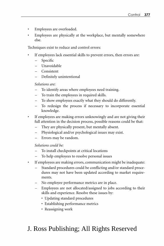
• Employees are overloaded.
• Employees are physically at the workplace, but mentally somewhereelse.
Techniques exist to reduce and control errors:
• If employees lack essential skills to prevent errors, then errors are:
– Specific
– Unavoidable
– Consistent
– Definitely unintentional
Solutions are:
– To identify areas where employees need training.
– To train the employees in required skills.
– To show employees exactly what they should do differently.
– To redesign the process if necessary to incorporate essentialknowledge.
• If employees are making errors unknowingly and are not giving theirfull attention in the decision process, possible reasons could be that:
– They are physically present, but mentally absent.
– Physiological and/or psychological issues may exist.
– Errors may be random.
Solutions could be:
– To install checkpoints at critical locations
– To help employees to resolve personal issues
• If employees are making errors, communication might be inadequate:
– Standard procedures could be conflicting and/or standard proce-dures may not have been updated according to market require-ments.
– No employee performance metrics are in place.
– Employees are not allocated/assigned to jobs according to theirskills and experience. Resolve these issues by:
• Updating standard procedures
• Establishing performance metrics
• Reassigning work
Control 377
J. Ross Publishing; All Rights Reserved

6.3.2 The Basic Error-Proofing ConceptFollowing fundamental rules can improve the error-proofing concept:
• Describe the error or defect the employee has made and provide thestatistics, if available, to the employee.
• Identify areas where there is the potential for error/defect and findways to minimize the areas where an error/defect has alreadyoccurred.
• Instruct employees to follow standard procedures.
• Establish checks and balances to minimize errors.
• Find the root cause(s) of errors by asking “why?” Find a solution byasking “how?”
• Use brainstorming sessions to find ideas to resolve errors/defects.
6.3.3 Error-Proofing ToolsGuidelines for designing a tool with the objective of minimizing errors/defectsinclude:
• If a tool detects an error while the error is being made, the tool is con-sidered to be a good tool.
• If a tool can predict a defect before the next operation, the tool is con-sidered to be a better tool.
• If a tool makes occurrence of an error impossible, the tool is consid-ered to be a best tool.
Although numerous tools are available for error proofing, commonly usedtools include:
• Sensors
• Checks and balances
• Templates
• Standard procedures/guides/references
• Sequence checks
• Critical condition indicators
• Mistake proofing
• A redesign process
• Create error-preventing devices:
– Simple process
378 Six Sigma Best Practices
J. Ross Publishing; All Rights Reserved

– Quick feedback loop
– Focused application
– Team of the right employees
These tools help businesses to reduce errors. Yet, two simple ways to minimizeerrors are:
• Prevent errors
• Mitigate errors
Prevent Errors—Errors may be prevented in several ways:
• Eliminate the possibility of errors. Install/utilize a tool that would pre-vent a system user from reaching a stage in which as error could occur,e.g., an automobile will not start until it is in “park.” This type of toolis generally known as “eliminate error possibility.”
• Delegate responsibility. An “easy way out” is to delegate the necessaryresponsibility to make decisions to someone else. Generally, this is nota good tool, but some employees may take advantage of it.
• Facilitate tasks. A very commonly used tool (concept) is to facilitatetasks. Achieving this concept can include:
– Task matching to an individual’s ability
– Task stratification
– Task specialization
– Task identification using different colors
• Detect errors. An error-detection tool is a commonly used tool, e.g., asmoke detection alarm.
Mitigate Errors—A variety of mitigating tools are available, e.g, the “auto filesaving” feature in Microsoft Office® software. Prevention guidelines include:
• Universal involvement in defect prevention
• Process improvement to eliminate, simplify, and/or combine opera-tions/activities/processes
• On-time production of products/services to minimize chances oferror
• Production based on demand or no extra production
If the team is not successful at maintaining process improvement gains usingthese tools and techniques, the next step is to utilize the SPC tool (statisticalprocess control).
Control 379
J. Ross Publishing; All Rights Reserved
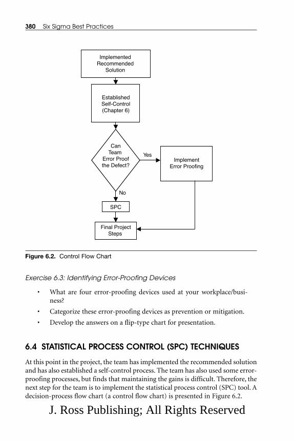
Exercise 6.3: Identifying Error-Proofing Devices
• What are four error-proofing devices used at your workplace/busi-ness?
• Categorize these error-proofing devices as prevention or mitigation.
• Develop the answers on a flip-type chart for presentation.
6.4 STATISTICAL PROCESS CONTROL (SPC) TECHNIQUES
At this point in the project, the team has implemented the recommended solutionand has also established a self-control process. The team has also used some error-proofing processes, but finds that maintaining the gains is difficult. Therefore, thenext step for the team is to implement the statistical process control (SPC) tool. Adecision-process flow chart (a control flow chart) is presented in Figure 6.2.
380 Six Sigma Best Practices
ImplementedRecommended
Solution
EstablishedSelf-Control(Chapter 6)
CanTeam
Error Proofthe Defect?
ImplementError Proofing
Yes
SPC
No
Final ProjectSteps
Figure 6.2. Control Flow Chart
J. Ross Publishing; All Rights Reserved
SPC is a problem-solving tool that may be applied to any process. SPC reflectsa desire of all individuals in the business/product/process group for a continuousimprovement in quality by the systematic reduction of variability. Although sev-eral available SPC tools are listed below, only the SPC control chart tool of SPCwill be discussed. (Some of these tools have already been discussed in previouschapters.)
• Cause-and-effect diagram
• Check sheet
• Defect-concentration diagram
• Histogram
• Pareto chart
• Scatter diagram
In the 1920s, Walter A. Shewhart of Bell Telephone Laboratories was a pioneerin the SPC field. Since World War II, W. Edward Deming and Joseph M. Juranhave been leaders in spreading statistical quality-control methods.
A control chart is a statistical device primarily used for studying, analyzing,and controlling repetitive processes. Control charts have key purposes:
• To define the goal or standard for a process that business leaders arestriving to attain
• To be used as a tool for attaining the defined goal
• To be used as a tool for evaluating whether or not a goal has beenachieved
Therefore, a control chart is a tool to be used for product/process specifica-tions, production, and inspection as needed to link and make interdependentthese phases in any business environment. The control chart tool of SPC will nowbe discussed in several subsections.
6.4.1 Causes of Variation in a ProcessPrimarily, variation is of two types—chance and special (or assignable). Chancevariation is due to inherent interaction among input resources. Industry recog-nizes that certain variations in the quality of product are due to chance variationsand that little can be done other than revise the process. This chance variation isthe sum of the effects of an entire complex of chance causes. In this complex ofcauses, the effect of each cause is slight and no major part of the total variationcan be traced to a single cause. The key to minimizing chance variations is to focuson a fundamental process change.
Control 381
J. Ross Publishing; All Rights Reserved
In addition to chance variation in quality, other variations are due to assign-able causes. These variations are relatively large and are attributable to special(assignable) causes. Input resources are typically the main source of assignablevariations. Assignable variations are generally unpredictable and are not “nor-mal.” Investigating the specific data points (information) related to the specialvariation is important. Develop solution(s) for a special variation, implement themost appropriate solution, and check the variation again. In summary, there aretwo types of variations:
• Chance
• Assignable Causes—Usually assignable-cause variations are due to:
– Differences in equipment, people, material, process/technology,and facility
– Differences in each of these factors over time
– Differences in their relationships to each other
Once the cause(s) of variation in a process is known, the next step is to deter-mine the SPCs impact on control of process performance.
6.4.2 Impact of SPCs on Controlling Process PerformanceControl limits in a control chart are generally based on establishing ± 3 sigma lim-its for the variable being measured. These control limits are not customer specifi-cation limits. A control chart serves several purposes:
• To define a goal or standard for a process with upper and lower con-trol limits, e.g., something a business might be striving to attain
• To be used as a tool for attaining the defined goal
• To be used as a judging tool of whether or not a goal has been reached
• To allow identification of unnatural (nonrandom) patterns in processvariables
• To track processes and product parameters over time
Advantages and disadvantages of using a control chart include:
Advantages:
• Effective in defect prevention
• A proven technique in quality and productivity improvement
• Provides process capability information
• A good diagnostic tool
• Can be used for independent and dependent variables
382 Six Sigma Best Practices
J. Ross Publishing; All Rights Reserved

Disadvantages:
• Not a simple tool; all users must be well trained and must participatein a continuing education (training) program
• Correct data must be collected
• Tool parameters (mean, standard deviation, range) must be calculatedcorrectly
• User must have good knowledge of how to analyze charts correctly
Process control activities can also be classified qualitatively from best to worstas shown in Table 6.1.1
Control 383
Table 6.1. Qualitative Classification of Process Control Activities
Category 1 — Implemented improvement will eliminate errorcondition from occurring; may be a long-termcorrective action from error-proofing or designchanges
Category 2 — Implemented improvement will detect whenerror condition occurs; “raising the flag” will stopthe equipment/process so that defect will notmove forward
Category 3 — If every participant is fully trained andunderstands SPC charts, once a chart signals aproblem, everyone must understand SPC rulesand agree to stop process for special issueidentification
Category 4 — Audit or inspection 100%; generally a short-termsolution
Category 5 — Same as Category 3 except participants do nothave authority to implement corrective action;team will need approval from management
Category 6 — Just to implement standard operatingprocedure; generally this type of action isdifficult to maintain
Category 7 — Utilization of warning signals to detect defects;frequency of ignoring these signals is generallyhigh
Category 8 — Implementing SPC without training theparticipants
BEST
WORST
J. Ross Publishing; All Rights Reserved

6.4.3 Control Chart Development Methodology andClassificationTypical steps are used to develop and analyze a Shewart control chart:
1. Select the appropriate response variable to chart.
2. Establish a rationale of data collection frequency for a subgroup andan appropriate sample size.
3. Select the appropriate control chart for the data.
4. Establish the data collection system.
5. Calculate the centerline and control limits (upper and lower).
6. Plot the data.
7. Check for out-of-control (OOC) conditions. A basic guidelineincludes:
• One or more data points outside the 3-sigma control limits
• Two of three data points outside the 2-sigma limit
• Four of five data points outside the 1-sigma limit
• Several consecutive data points (six to eight) on one side of thecenterline
• Once the process leaders have defined the warning limits, and ifone or more points are in the “neighborhood” of a warning limit,then this suggests the need to collect more data immediately tocheck for the possibility of the process being out of control.
8. Interpret findings, investigate cause(s) for variation, and proposeand implement solution.
Control Chart ClassificationControl charts are classified for measurements (continuous) and attributes (dis-crete), depending on if the observations on the quality characteristic are measure-ments or enumeration data. As an example, we may choose to measure thediameter of a hole in a component, e.g., with a micrometer, and utilize these datato develop a control chart for measurement. On the other hand, we may judgeeach unit of this product as either defective or not defective and use the fractionof defective units found or the total number of defects in relation to a controlchart for attributes. Classification of a control chart is presented in Figure 6.3. Thefollowing is a short description of control charts:
• X & MR Chart—This chart is also known as an individuals and a mov-ing-range chart. This chart plots each individual collected value perproduct and a moving average. This chart is similar to a X-bar & Rchart.
384 Six Sigma Best Practices
J. Ross Publishing; All Rights Reserved

• Xbar & R Chart and Xbar & Sigma Chart—Control chart develop-ment over an average quality is known as an X-bar chart. Range (R)charts measure the gain or loss of uniformity within each subgroupthat represents the variability in the response over time. R charts arebased on the range of values within each subgroup. Process variabil-ity is tracked through sigma charts that are based on the standarddeviation (SD) within each subgroup.
• p Chart—This is a simple chart that is used to track the number ofnonconforming units for a constant sample size as well as for a vari-able sample size.
Control 385
Continuous orDiscrete Data?
Continuous Discrete
Is SampleSize = 1? X & MR
Chart
Yes
No
Very Small
SampleSize?
Z-MRShort Run
SPC
Yes
Is SampleSize <8?
No
X-bar & RChart
Yes
X-bar & s
No
Measuring 1 orMore Defects
per UnitOne
Defect
Are AllSubgroups
Equal inSize?
Yes No
p or npCharts
p Chart
MorethanOneDefect
Are AllSubgroupsEqual in
Size?
c Chart
Yes
u Chart
No
Data Collection
Figure 6.3. Control Chart Classification
J. Ross Publishing; All Rights Reserved

• c Chart—This is a simple chart that is used to track the number ofdefects per unit with the assumption that the sample size is constant.
• u Chart—A u chart is similar to a c chart with the assumption that thesample size is both fixed and variable.
Control Chart Hypothesis TestingThe hypothesis testing concept is presented in Figure 6.4. Lower control limit(LCL) and upper control limit (UCL) represent the boundaries for the nonrejec-tion area of H0 and the areas that lie outside these limits represent H0 rejectionareas at α level of significance.
Assuming that the process mean and standard deviation (SD), e.g., μ and σ,are known, and, furthermore, assuming that the quality characteristic follows thenormal distribution, let ⎯X = sample mean based on random sample of size n.
Then, the probability is (1 – α) that the mean of such random sample will fallbetween μ + Zα/2(σ/√n) and μ – Zα/2(σ/√n).
6.4.4 Continuous Data Control ChartsThis subsection will describe several charts that present the Continuous Data andBox-Cox Transformation Methods.
Continuous Data for IndividualsCollected (measured) data for the individuals must be tested for normality beforeusing the calculated lower (LCL) and upper control limits (UCL) based on stan-dard formulas. If the distribution is skewed on either side (positive or negative),the control limits for individuals must be calculated based on area distributiontables. The theoretical limits will be calculated using standard deviations (SDs)from the mean. Values of X and R can have substantial variability because there isonly one individual value per subgroup. The number of subgroups should belarge, e.g., 100 or more.
386 Six Sigma Best Practices
CannotReject H0
Reject H0
α/2
α/2
H0: Mean = X
X
**
*
*
*
**
**
Time
Lower Control Limit
Upper Control Limit
Reject H0
Figure 6.4. Control Chart Hypothesis Testing
J. Ross Publishing; All Rights Reserved

Box-Cox TransformationBox-Cox transformation is a commonly used method to normalize data. Box-Coxtransformation will manipulate non-normal data and suggest the appropriate fac-tor to be used to change the collected data into normal data. Yet, correcting non-normal data is not always necessary unless the data are highly skewed. Controlcharts work well even if the data are not normally distributed; therefore, accord-ing to Wheeler2 and Wheeler and Chambers,3 transforming data are not requiredif the data are used in control charts. Therefore, a user must use care when decid-ing to use Box-Cox transformation.
MINITAB software can provide Box-Cox transformation of data in two situ-ations:
• Individual observations or subgroup data
• Power transformation for other conditions—Xbar, R, S, Xbar-R,Xbar-S, individual moving range, EWMA, moving average, Z-MR,etc. (Details are available in books on MINITAB.)
Individual Observations or Subgroup Data Transformation—This is goodprocedure for positive data only. The MINITAB procedure is as follows:
Step 1. Choose the commands Stat > Control > Box-Cox transformation. Themenu screen will come up.
Step 2. Choose one of the following:
• If subgroups or individual data are in one column, enter the data col-umn in Single Column. In Subgroup size, enter a subgroup size or acolumn of subgroup indicators. If data are individual observations,enter a subgroup size of 1.
• For a subgroup in rows, enter a series of columns in Subgroups acrossrows of.
Step 3. At this point, a command can be used in one of the following ways:
• To establish the best lambda (λ) value for the transformation, clickOK.
• To establish the best λ value for the transformation, transform thedata, and store the transformed data in the column(s) you specify. Todo this, in Store transformed data in, enter a column (or columns) inwhich to store the transformed data, and then click OK.
• To transform the data with a λ value, enter and store the transformeddata in a column (or columns) you specify. To do this, in Store trans-formed data in, enter column(s) in which to store the transformed
Control 387
J. Ross Publishing; All Rights Reserved

data. Click Options, in Use lambda, enter a value. Click OK in eachdialog box.
Box-Cox transformation estimates the λ value, which minimizes the standarddeviation (SD) of a standardized transformed variable.
When:
λ ≠ 0, the resulting transformation is Yλ
λ = 0, the resulting transformation is loge Y
Some specific relationships4 for the different values of λ are presented inTable 6.2A.
The sample data in Table 6.2B are used to show how to use the MINITAB toolto obtain the λ value. A sample of gas mileage data for 70 automobiles was col-lected and reorganized in range groups as presented in Table 6.2B.
Gas mileage frequency data for the automobiles are plotted and presented inFigure 6.5A in histogram form, which shows that the mileage frequency data areskewed to the right. A second chart is presented in Figure 6.5B, which is a Box-Cox plot for the λ values.
Interpreting the Box-Cox λ plot: The “Last Iteration Information” table (inFigure 6.5B) contains the best estimate of λ, which is Est = 0.562, Low = 0.506,and Up = 0.618. A 95% confidence interval for the “true” value of λ is designatedby vertical lines on the graph in Figure 6.5B. Although the best estimate of λ is0.562, in practical situations, a λ value is wanted that corresponds to an under-standable transformation, such as the square root (for λ = 0.5). In this example,the value of λ = 0.5 is a reasonable choice because it falls within the 95% confi-dence interval. All λ values in the 95% confidence interval are less than or equalto the horizontal dashed line in Figure 6.5B. Therefore, any λ value that has a stan-dard deviation close to the dashed line is also reasonable to use for the transfor-mation. In this example, this corresponds to an interval of 0.2 to 1.1.
MINITAB ChartsMINITAB software can provide four types of continuous data control charts:
• Moving Average Chart—Unweighted moving averages
• Exponentially Weighted Moving Average Chart (EWMA)—Exponentially weighted moving averages
• Cumulative Sum Chart (CUSUM)—Cumulative sum of the devia-tions of each sample value from the target value
• Zone Chart—Assigns a weight to each point, depending on its dis-tance from the centerline, and plots the cumulative scores
388 Six Sigma Best Practices
J. Ross Publishing; All Rights Reserved
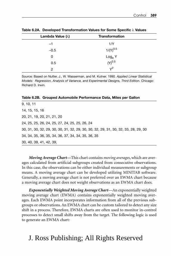
Moving Average Chart—This chart contains moving averages, which are aver-ages calculated from artificial subgroups created from consecutive observations.In this case, the observations can be either individual measurements or subgroupmeans. A moving average chart can be developed utilizing MINITAB software.Generally, a moving average chart is not preferred over an EWMA chart becausea moving average chart does not weight observations as an EWMA chart does.
Exponentially Weighted Moving Average Chart—An exponentially weightedmoving average chart (EWMA) contains exponentially weighted moving aver-ages. Each EWMA point incorporates information from all of the previous sub-groups or observations. An EWMA chart can be custom tailored to detect any sizeshift in a process. Therefore, EWMA charts are often used to monitor in-controlprocesses to detect small shifts away from the target. The following logic is usedto generate an EWMA chart:
Control 389
Table 6.2A. Developed Transformation Values for Some Specific λ Values
Lambda Value (λ) Transformation
–1 1/Y
–0.5 1/(Y)0.5
0 Loge Y
0.5 (Y)0.5
2 Y2
Source: Based on Nutter, J., W. Wasserman, and M. Kutner. 1990. Applied Linear StatisticalModels: Regression, Analysis of Variance, and Experimental Designs, Third Edition. Chicago:Richard D. Irwin.
Table 6.2B. Grouped Automobile Performance Data, Miles per Gallon
9, 10, 11
14, 15, 15, 16
20, 21, 19, 20, 21, 21, 20
24, 25, 25, 26, 24, 25, 27, 24, 25, 25, 26, 24
30, 31, 30, 32, 29, 30, 30, 31, 32, 29, 30, 30, 32, 29, 31, 30, 32, 33, 28, 29, 30
34, 34, 35, 36, 35, 34, 36, 37, 34, 34, 35, 36, 35
30, 40, 39, 41, 42, 39,
J. Ross Publishing; All Rights Reserved

390 Six Sigma Best Practices
10 20 30 40
0
5
10
Automobile Performance, Miles/Gallon
Fre
quen
cy
–1.0 –0.5 0.0 0.5 1.0 1.5 2.0 2.5 3.0 3.5 4.0 4.5 5.0
1.0
1.5
2.0
2.5
SD
95% Confidence Interval
Lambda
Last Iteration InformationLambda SD
Low 0.506 1.083
Est 0.562 1.082
Up 0.618 1.082
Figure 6.5A. Frequency Histogram: Automobile Performance, Miles per Gallon
Figure 6.5B. Box-Cox Plot for the Lambda (λ) Values
J. Ross Publishing; All Rights Reserved

Let:
Zi = Data group i
then,
Zi = w ⎯Xi + (1 – w) Zi–1
or the general expression:
Zi = w ⎯Xi + w(1 – w) ⎯Xi-1 + w(1 – w)2 ⎯Xi-2 + ... + w(1 – w)i-1 ⎯X1 + (1 – w)i ⎯X0
where:
w = Weight
⎯Xi = Mean of subgroup i
⎯X0 = Mean of all data
Example 6.1: Developing an EWMA Chart
Use the eight individual measurements as presented in Table 6.3 to develop anEWMA chart, using the weight factor of 0.25.
Solution:The chart in Figure 6.6 has been developed using MINITAB software. The com-mands are as follows:
Stat > Control chart >EWMA
The data are stored in one column “Subgroup Mean,” therefore, select
Single Column: “Subgroup Mean”
Weight for EWMA: 0.25
OK
Figure 6.6 is based on the following calculations, which are performed byMINITAB software in the background:
Mean of all the data:
⎯X0 = (13 + 8 + 7 + 9 + 12 + 6 + 8 + 10)/8 = 9.125
Control 391
Table 6.3. Individual Measurements for Selected Subgroups
Subgroup 1 2 3 4 5 6 7 8
Measurement 13 8 7 9 12 6 8 10
J. Ross Publishing; All Rights Reserved

Zi = w ⎯Xi + (1 – w) Zi–1
Z1 = w ⎯ ⎯X1 + (1 – w) ⎯X0
Z1 = (0.25) (13) + (1 – 0.25)(9.125)= 10.094
Z2 = w ⎯X2 + w(1 – w) ⎯X1+ (1 – w)2 ⎯X0
Z2 = (0.25)(8) + (0.25)(1 – 0.25)(13) + (1 – 0.25)2(9.125)= 9.57
Similarly, the remaining values as presented here may be checked: Z3 = 8.93; Z4 =8.95; Z5 = 9.71; Z6 = 8.78; Z7 = 8.59; and Z8 = 8.94.
Cumulative Sum Chart—A cumulative sum chart (CUSUM) plots thecumulative sums of the deviations of each sample value from the target value. TheCUSUM plotted chart is based on the subgroup means or the individual observa-tions. Once a process is in-control, a CUSUM chart (as well as an EWMA chart)is a good device to use to detect small shifts from the target. Detailed explanationsas well as instructions about developing a CUSUM chart may be found in aMINITAB tool book.
Zone Chart—A zone chart is a hybrid of the ⎯X (or individuals) chart and theCUSUM chart. Zone charts are usually preferred over ⎯X charts because zonecharts are simple. Detailed explanations and instructions about developing a zonechart may be found in a MINITAB tool book.
392 Six Sigma Best Practices
87654321
12.5
11.5
10.5
9.5
8.5
7.5
6.5
5.5
Sample Number
EW
MA
Mean=9.125
UCL=12.13
LCL=6.124
Figure 6.6. EWMA Chart for Subgroups
J. Ross Publishing; All Rights Reserved

Other Charts—Other continuous data control charts include:
• Z-MR Chart
• Xbar and R Chart
• Xbar and s Chart
Z-MR Chart—If enough data do not exist in each run to produce good esti-mates of process parameters, use a Z-MR chart. Measurement data are standard-ardized by subtracting the mean to the center of the data, then dividing by thestandard deviation (Z = (X – μ)/σ). Standardizing allows data collected from dif-ferent runs to be evaluated by interpreting a single control chart.
The MINITAB tool can be used to estimate the process means and the stan-dard deviations:
• Estimating the Process Mean—A Z-MR chart estimates the mean foreach different component or product separately. It pools all the datafor a common component and obtains the average of the pooled data.The result is an estimate of μ for that component.
• Estimating the Process Standard Deviation—A Z-MR chart providesfour methods for estimating σ, the process standard deviation (SD)(Table 6.4). Details of the four methods may be found in a MINITABbook.
Generally, the By component method (see Table 6.4) is a good choice when ateam has very short runs and wants to combine runs of the same component toobtain a more reliable estimate of σ. If the runs are sufficiently long, the By com-ponent method can also provide good estimates of σ.
The estimation method choosen by a team will be determined by assump-tions that the team is willing to make about the variation of their process.Guidance for selection is presented in Table 6.4. A Z-MR chart estimates the meanfor each different component or product separately. The mean of a component iscalculated in a Z-MR chart by averaging all the data for that component. Thisaverage is the estimate of μ for that component.
Example 6.2: Developing a Z-MR Chart
A machining department produces a power transmission shaft in batches of threeunits. Shaft diameter data were collected from five runs as presented in Table 6.5.Develop a Z-MR chart from the data.
Solution:A Z-MR chart has been developed using the MINITAB tool. The chart is pre-sented in Figure 6.7.
Control 393
J. Ross Publishing; All Rights Reserved

Xbar and R Charts—Xbar and R charts are generally utilized to track theprocess level and process variation for a sample size less than 8, while Xbar and scharts are used for larger samples. A user analyzing the charts will be able to detectthe presence of special causes.
In MINITAB, Xbar and R charts base the estimate of the process variation σon the average of the subgroup ranges. A user can also use a pooled standard devi-ation or enter an historical value for σ.
The Xbar and R charts are utilized to analyze several critical points:
• The Xbar chart shows how a process is working and where the processis centered.
• If there is an impact of natural variation only, the Xbar chart willshow that the center of the process is not shifting significantly.
394 Six Sigma Best Practices
Table 6.4. The Process Standard Deviation’s Estimating Methods
Method When … Which does this …
Constant: pool all All output from Pools all data across runs anddata process has the same components to obtain a
variance regardless of common estimate of σsize of measurement
Relative to size: Variance increases in a Takes natural log of data,pool all data, use fairly constant manner pools transformed data acrosslog (data) as size of measurement all runs and all components, and
increases obtains a common estimate of σ for transferred data; naturallog tranformation stabilizes thevariation in cases where variationincreases as size of measurementincreases
By component: All runs of a particular Combines all runs of samepool all runs of component or product component or product same component/ have same variance to estimate σbatch
By run: no Cannot assume all runs Estimate σ for each runpooling of a particular independently
component or product have same variance
J. Ross Publishing; All Rights Reserved

• If the Xbar chart shows a trend in which the center of the process ismoving gradually up or down, a good probability exists that thismovement is due to assignable causes.
• If the Xbar chart is erratic and out of control, then something ischanging the center rapidly and inconsistently.
• If the Xbar chart and R chart are both out of control, first look for theissues affecting the R chart.
• If the R chart is out of control, it can affect the Xbar chart as well. Ifthe R chart is out of control, this is also an indication that somethingis not operating in a uniform manner.
• If the R chart is narrow, the product is uniform.
Example 6.3: Developing Xbar and R Charts
The camshaft department of a bus manufacturing company manufactures apower transmission shaft that is 25 ± 0.1 in. long. The bus assembly departmentis complaining that the power transmission shaft is not produced to specifica-tions. As a result of the complaints, management wants to run Xbar and R chartsto monitor the length characteristic of the shaft.
Control 395
Table 6.5. Sampled Collected Data forShaft Diameter
Job Run, # Shaft Diameter, in.
1 2.0121 2.0051 2.0502 2.0102 2.0702 2.0903 2.0153 2.0193 2.0524 2.0354 2.0454 2.0305 2.0405 2.0105 2.035
J. Ross Publishing; All Rights Reserved

The data in Table 6.6 have been collected in ten subgroups with five datapoints in each subgroup. Develop Xbar and R charts and test as follows:
• One point or less that is more than 3 sigma from the centerline
• Six points in a row, all increasing or all decreasing
• Two out of three points that are more than 2 sigma from the center-line (while all of these three points are on the same side)
• Four out of five points that are more than 1 sigma from the centerline(on same side)
Solution:Xbar and R charts have been developed using MINITAB software with ± 3σ con-trol limits in Figure 6.8.
Interpreting the results: The centerline on the Xbar chart is at 25.03, imply-ing that the process is falling within the specification limits. The centerline on theR chart, 0.105, is slightly larger than the maximum allowable variation of ± 0.1 in.This excess may indicate variability in the process.
Two additional groups of charts have been developed using MINITAB soft-ware. They are presented in Figures 6.9 and 6.10 (Xbar and R charts with ± 2σcontrol limits and ± 1σ control limits, respectively).
Xbar and s Chart—Although Xbar and R charts are used for smaller samples,Xbar and s charts are typically used to track process variation for sample sizes
396 Six Sigma Best Practices
0
1 2 3 4 5
10 155Subgroup
Sta
ndar
dize
d D
ata
Mean = 0
UCL = 3
LCL = –3
0
1
2
3
4
Mov
ing
Ran
ge
R = 1.128
LCL = 0
UCL = 3.686
Figure 6.7. Z-MR Chart for Shaft Diameter
J. Ross Publishing; All Rights Reserved

larger than seven. Because both charts are plotted together, a user can track boththe process level and the process variation at the same time, as well as detect thepresence of special causes. (No example is presented here, but MINITAB softwarecan be used to plot Xbar and s charts.)
6.4.5 Discrete Data Control ChartsDiscrete data control charts are similar in structure to continuous data controlcharts, except that these charts plot statistics from count data rather than frommeasurement data, e.g., a product may be compared against a standard and clas-sified as being either defective or not defective. The number of defects may alsoclassify products.
A process statistic, e.g., the number of defects, is plotted vs. sample numberor time in variables control charts. The centerline represents the average statistic.The upper (UCL) and lower control limits (LCL) are drawn, by default, 3 σ aboveand below the centerline.
A process is in-control when most of the points fall within the bounds of thecontrol limits and the points display no nonrandom patterns.
The p, c, and u charts will now be discussed.
• p Chart
• p Chart with Varying Sample Size
• c Chart
• u Chart
• u Chart with Varying Sample Size
Control 397
Table 6.6. Length Data for Shaft
Subgroup Shaft Length, in.
1 25.02, 25.00, 25.05, 24.95, 24.99
2 25.07, 25.12, 24.99, 24.98, 25.05
3 24.98, 25.01, 25.07, 25.04, 24.99
4 24.95, 24.99, 24.98, 24.99, 25.05
5 25.02, 25.01, 25.05, 25.07, 25.02
6 25.09, 25.01, 25.07, 25.05, 25.06
7 25.02, 25.01, 25.09, 25.11, 25.12
8 24.97, 24.95, 24.99, 25.05, 25.09
9 24.99, 24.95, 25.01, 25.05, 24.98
10 25.12, 25.04, 25.01, 24.99, 25.00
J. Ross Publishing; All Rights Reserved

398 Six Sigma Best Practices
10987654321Subgroup
0
25.10
25.05
25.00
24.95
Sam
ple
Mea
n
Mean = 25.03
UCL = 25.09
LCL = 24.96
0.2
0.1
0.0
Sam
ple
Ran
ge
R = 0.105
UCL = 0.2220
LCL = 0
Figure 6.8. Developed Xbar and R Chart for Shaft Length
10987654321Subgroup 0
Sam
ple
Mea
n
Mean = 25.03
2.0SL = 25.07
–2.0SL = 24.98
0.2
0.1
0.0
Sam
ple
Ran
ge
R = 0.105
2.0SL = 0.1830
–2.0SL = 0.02699
25.0825.0725.0625.0525.0425.0325.0225.0125.0024.9924.98
Figure 6.9. Additional Xbar and R Chart for Example 6.3 at ± 2.0SL
J. Ross Publishing; All Rights Reserved
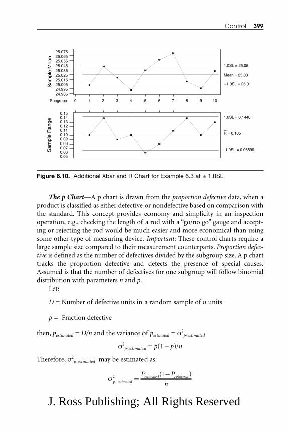
The p Chart—A p chart is drawn from the proportion defective data, when aproduct is classified as either defective or nondefective based on comparison withthe standard. This concept provides economy and simplicity in an inspectionoperation, e.g., checking the length of a rod with a “go/no go” gauge and accept-ing or rejecting the rod would be much easier and more economical than usingsome other type of measuring device. Important: These control charts require alarge sample size compared to their measurement counterparts. Proportion defec-tive is defined as the number of defectives divided by the subgroup size. A p charttracks the proportion defective and detects the presence of special causes.Assumed is that the number of defectives for one subgroup will follow binomialdistribution with parameters n and p.
Let:
D = Number of defective units in a random sample of n units
p = Fraction defective
then, pestimated = D/n and the variance of pestmated = σ2p-estimated
σ2p-estimated = p(1 – p)/n
Therefore, σ2p-estimated may be estimated as:
σ p estimatedestimated estimatedP P
n− =−2 1( )
Control 399
10987654321Subgroup 0
25.07525.06525.05525.04525.03525.02525.01525.00524.99524.985
Sam
ple
Mea
n
Mean = 25.03
1.0SL = 25.05
–1.0SL = 25.01
0.150.140.130.120.110.100.090.080.070.060.05
Sam
ple
Ran
ge
R = 0.105
1.0SL = 0.1440
–1.0SL = 0.06599
Figure 6.10. Additional Xbar and R Chart for Example 6.3 at ± 1.0SL
J. Ross Publishing; All Rights Reserved

The centerline and control limits for the proportion defective (fraction defec-tive) can be calculated as follows:
Let:
m = Number of samples and
n = Number of units in a sample (as defined earlier)
then,
and
Example 6.4: Developing a p Chart with MINITAB Software
Part X has quality issues. Receiving and Inspection receive part X from a supplierdaily. Data for received lots for the last 2 weeks are presented in Table 6.7. Developa p chart utilizing the MINITAB software tool.
Solution:
⎯p = (5 + 6 + 7 + 8 + 9 + 7 + 5 + 6 + 7 + 6)/(10 � 100)
= 0.066
UCL = 0.066 + 3 × √((0.066) (1 – 0.066))/100
= 0.1405
LCL = 0
LCL pp p
n= −
−( )3
1
UCL pp p
n= +
−( )3
1
pD
m n= ∑
��
400 Six Sigma Best Practices
Table 6.7. Receiving and Inspection Data for Part X for a Two-Week Period(Fixed Sample Size)
Lot Size: 100 100 100 100 100 100 100 100 100 100
Part Failed: 5 6 7 8 9 7 5 6 7 6
J. Ross Publishing; All Rights Reserved

The chart developed with MINITAB software is presented in Figure 6.11. Allsamples are in control. From a Six Sigma quality improvement point of view, theSigma metrics is at 3.0 sigma, indicating room for improvement still exists.Appropriate steps should be taken to investigate the process and determine rootcauses of variation. Once defect types are known, process changes should beimplemented.
The p Chart with Varying Sample Size—The previous section that describedthe p chart was greatly simplified because the sample size taken was constant. Inmany situations, having a fixed sample size is not necessary.
Let:
Di = Number of defective units in a random sample of ni units, i = 1, 2, ..., m
ni = Number of units in sample i
m = Total number of samples
pi = Fraction defective in sample i
then,
pi = Di /ni
The centerline and control limits for the fraction defective chart can be cal-culated as follows:
Control 401
109876543210
0.15
0.10
0.05
0.00
Sample Number
Pro
port
ion
P = 0.066
UCL = 0.1405
LCL = 0
Figure 6.11. p Chart for Receiving Part Quality with Fixed Sample Size
J. Ross Publishing; All Rights Reserved

Let:
⎯p = Centerline
then,
, i = 1, 2, . . ., m
Because MINITAB software calculates the value of ⎯p based on a simple aver-age, the above logic is based on simple average calculations. Important: A simpleaverage of the fraction defective per unit of each sample is not taken. To work withthese data, a weighted average must be taken. The weighted average can be calcu-lated as follows:
Let:
M = Total unit count in m samples
= Σni, i = 1, 2, 3, . . ., m
Then,, i = 1, 2, . . ., m
Control limits for the p chart are as follows:
Control limits for each sample can be calculated as follows:
LCL pp p
M
n
= −−( )
31
UCL pp p
M
n
= +−( )
31
pn
Mpi
ii
=⎛
⎝⎜⎜⎜⎜
⎞
⎠⎟⎟⎟⎟
⎡
⎣⎢⎢
⎤
⎦⎥⎥∑
p
D
n
m
i
i=
⎛
⎝⎜⎜⎜⎜
⎞
⎠⎟⎟⎟⎟∑
402 Six Sigma Best Practices
J. Ross Publishing; All Rights Reserved

This logic has been applied in Example 6.5.
Example 6.5: Developing a p Chart with a Variable Sample Size (n)
Part X has some quality issues. Receiving and Inspection receives part X from asupplier daily. Data for received parts for the last 2 weeks are presented in Table6.8. Develop a p chart utilizing the MINITAB software tool.
Solution:If the centerline is based on a simple average, then,
= (5+6+7+8+9+7+5+6+7+6)/(100+115+95+120+118+99+105+120+119+110)
= 66/1101
= 0.05995
If the centerline is based on a weighted average, then,
The in-process data are presented in Table 6.9. The weighted p = 0.0601.
pn
Mpi
ii
=⎛
⎝⎜⎜⎜⎜
⎞
⎠⎟⎟⎟⎟
⎡
⎣⎢⎢
⎤
⎦⎥⎥∑
p
D
n
m
i
i=
⎛
⎝⎜⎜⎜⎜
⎞
⎠⎟⎟⎟⎟∑
LCL pp p
npi
i
– = −−( )
31
UCL pp p
npi
i
– = +−( )
31
Control 403
Table 6.8. Receiving and Inspection Data for Part for a Two-Week Period(Varying Sample Size)
Lot Size: 100 115 95 120 118 99 105 120 119 110
Part Failed: 5 6 7 8 9 7 5 6 7 6
J. Ross Publishing; All Rights Reserved

The p chart’s upper control limit (UCL) is calculated using a simple average(since MINITAB software is used):
= 0.05995 + 3 √ ((0.05995(1 – 0.05995))/(1101/10))
= 0.1278
Similarly, LCL = 0.
Control limits can be calculated for each sample.
Sample 1. Where, n1 = 100.
Then,
and
UCL–p1 = 0.05995 + 3 √ ((0.05995(1 – 0.05995))/100)
= 0.13117
and
LCL–p1 = 0
UCL pp p
np− = +−( )
1 31
1
UCL pp p
M
m
= +−( )
31
404 Six Sigma Best Practices
Table 6.9. In-process Data for the Weighted ⎯p Calculation
ni 100 115 95 120 118 99 105 120 119 110
Di 5 6 7 8 9 7 5 6 7 6
pi 0.05 0.052 0.074 0.067 0.076 0.071 0.048 0.05 0.059 0.055
pi-est 0.00454 0.00543 0.00639 0.0073 0.00815 0.00638 0.00458 0.00545 0.00638 0.0055
J. Ross Publishing; All Rights Reserved

Sample 2. Where, n2 = 115.
UCL–p2 = 0.12636
and
LCL–p2 = 0
Similarly, the control limits for the remaining samples can be calculated.
A chart developed with MINITAB software is presented in Figure 6.12. Allsamples are in control. From a Six Sigma quality improvement point of view, theSigma metrics is at 3.0 sigma, indicating room for improvement still exists.
The c Chart—At times, controlling the number of defects in a unit product ismore critical than controlling the proportion defective (fraction). In this circum-tance, a c chart should be used (as a control chart) for defects, e.g., when produc-ing a roll of sheet material, controlling the number of defects per foot isimportant. When the number of defects is linked to a per-unit-of-measurementsituation, then the Poisson distribution model should be used with parameter λ.Both the mean and variance of this distribution are also λ.
Let:
ci = Number of defects in unit i, i = 1, 2, 3, . . ., n
n = Number of units used in the test
Control 405
109876543210
0.15
0.10
0.05
0.00
Sample Number
Pro
port
ion
P = 0.05995
UCL = 0.1278
LCL = 0
Figure 6.12. p Chart for Receiving Part Quality with Variable Sample Size
J. Ross Publishing; All Rights Reserved

Then, the centerline of the control chart is
and
are the upper and the lower control limits, respectively. See Example 6.6 for howto develop a c chart.
LCL c c= −3
UCL c c= +3
cc
ni= ∑
406 Six Sigma Best Practices
Table 6.10. Sample Data of Identified Components’Characteristics
Identified Defective Count of DefectiveComponent Characteristics Characteristics
1 2, 4, 1 32 1, 4, 5 33 1, 2 24 2, 4 25 2, 3, 4, 5 46 1, 2, 3 37 4, 5 28 3, 4, 5 39 2, 3, 4 3
10 1, 2 211 4 112 3, 5 213 1, 2, 5 314 1, 2, 4 315 2, 3, 4 316 3, 4 217 1, 2, 4, 5 418 2, 4, 5 319 1, 3, 4 320 3, 5 2
J. Ross Publishing; All Rights Reserved

Example 6.6: Calculating the Centerline and Control Limits for a cChart and Plotting the Chart using MINITAB
A manufactured component has five identified characteristics to be inspected (1,2, 3, 4, and 5). Inspection data are presented in Table 6.10. The data identify resultsof inspecting the characteristics of 20 components. Calculate the centerline andcontrol limits for a c chart. Plot the chart using MINITAB software.
Solution:The centerline of the control chart is ⎯c :
⎯c = 53/20 = 2.65
and the upper (UCL) and lower (LCL) limits are
UCL = 2.65 + 3 √2.65 = 7.534
LCL = 2.65 – 3 √2.65 = 0
The c chart is plotted using MINITAB software (Figure 6.13). Based on theplotted chart, the process appears to be under control. However, 2.65 defectivecharacteristics per component out of five is too many. The process could beimproved.
The u Chart—The u chart is utilized when sample defects data are collectedfrom n components in the sample. Working with the number of defects per unitrather than with the total number of defects is preferable.
Control 407
20100
8
7
6
5
4
3
2
1
0
Sample Number
Sam
ple
Cou
nt
C = 2.65
UCL = 7.534
LCL = 0
Figure 6.13. c Chart for Several Specification Characteristics Failure
J. Ross Publishing; All Rights Reserved

Let:
n = Number of units in the sample
c = Total number of defects in the sample
u = Average number of defects per unit
m = Number of samples
where: u1, u2, u3, . . ., um are defects per unit for sample i = 1, 2, 3, . . ., m, respec-tively.
Then,
⎯u = Centerline on the u chart
and
, i = 1, 2, 3, . . ., m um
ui= ( )∑1
408 Six Sigma Best Practices
Table 6.11. Sample Data of Component’s Characteristics
Number ofCharacteristics Defects
Sample Sample size, n Unacceptable per Unit
1 7 5 0.7172 7 7 1.0003 7 6 0.8574 7 4 0.5715 7 8 1.1436 7 10 1.4297 7 6 0.8578 7 9 1.2869 7 11 1.571
10 7 4 0.57111 7 7 1.00012 7 8 1.14313 7 5 0.71714 7 9 1.28615 7 10 1.429
J. Ross Publishing; All Rights Reserved

and the control limits,
Example 6.7. Developing a u Chart
A u chart is to be constructed for the component characteristics data in Table 6.11.There are seven components in each sample (n = 7). Calculate the centerline,UCL, and LCL for a u chart. Utilize the MINITAB software tool to plot the u chart.
Solution:The centerline for the u chart:
⎯u = (1/15) (15.577)= 1.0385
The upper (UCL) and lower (LCL) control limits:
UCL = 1.0385 + 3 √(1.0385/7) = 2.194
LCL = 1.0385 – 3 √(1.0385/7) = 0
LCL uu
n= −3
UCL uu
n= +3
Control 409
151050
2
1
0
Sample Number
Sam
ple
Cou
nt
U = 1.038
UCL = 2.193
LCL = 0
Figure 6.14. u Chart of Characteristics Failure per Unit for Selected Components
J. Ross Publishing; All Rights Reserved
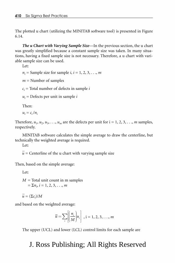
The plotted u chart (utilizing the MINITAB software tool) is presented in Figure6.14.
The u Chart with Varying Sample Size—In the previous section, the u chartwas greatly simplified because a constant sample size was taken. In many situa-tions, having a fixed sample size is not necessary. Therefore, a u chart with vari-able sample size can be used.
Let:
ni = Sample size for sample i, i = 1, 2, 3, . . ., m
m = Number of samples
ci = Total number of defects in sample i
ui = Defects per unit in sample i
Then:
ui = ci /ni
Therefore, u1, u2, u3, . . ., um are the defects per unit for i = 1, 2, 3, . . ., m samples,respectively.
MINITAB software calculates the simple average to draw the centerline, buttechnically the weighted average is required.
Let:
⎯u = Centerline of the u chart with varying sample size
Then, based on the simple average:
Let:
M = Total unit count in m samples= Σni, i = 1, 2, 3, . . ., m
⎯u = (Σci)/M
and based on the weighted average:
, i = 1, 2, 3, . . ., m
The upper (UCL) and lower (LCL) control limits for each sample are
un
Mui
ii
=⎛
⎝⎜⎜⎜⎜
⎞
⎠⎟⎟⎟⎟
⎡
⎣⎢⎢
⎤
⎦⎥⎥∑
410 Six Sigma Best Practices
J. Ross Publishing; All Rights Reserved
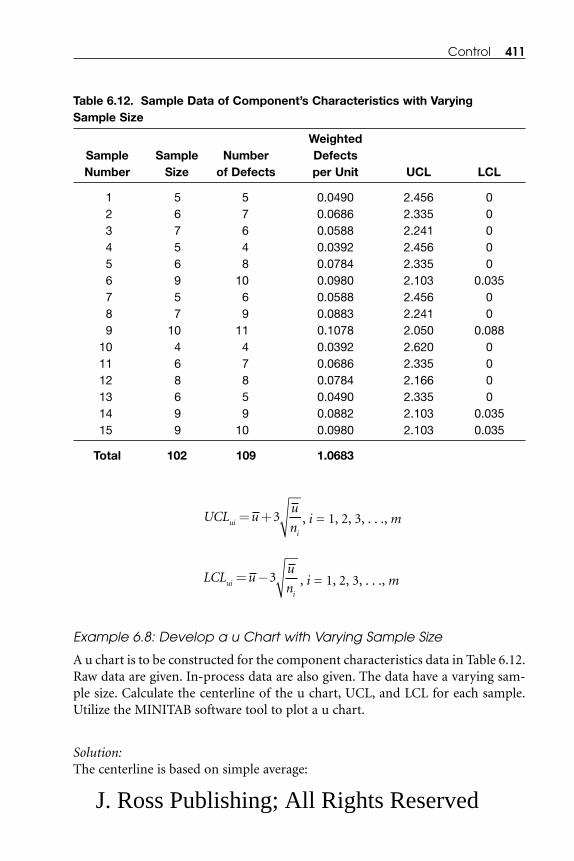
, i = 1, 2, 3, . . ., m
, i = 1, 2, 3, . . ., m
Example 6.8: Develop a u Chart with Varying Sample Size
A u chart is to be constructed for the component characteristics data in Table 6.12.Raw data are given. In-process data are also given. The data have a varying sam-ple size. Calculate the centerline of the u chart, UCL, and LCL for each sample.Utilize the MINITAB software tool to plot a u chart.
Solution:The centerline is based on simple average:
LCL uu
nui
i
= −3
UCL uu
nui
i
= +3
Control 411
Table 6.12. Sample Data of Component’s Characteristics with Varying Sample Size
WeightedSample Sample Number DefectsNumber Size of Defects per Unit UCL LCL
1 5 5 0.0490 2.456 02 6 7 0.0686 2.335 03 7 6 0.0588 2.241 04 5 4 0.0392 2.456 05 6 8 0.0784 2.335 06 9 10 0.0980 2.103 0.0357 5 6 0.0588 2.456 08 7 9 0.0883 2.241 09 10 11 0.1078 2.050 0.088
10 4 4 0.0392 2.620 011 6 7 0.0686 2.335 012 8 8 0.0784 2.166 013 6 5 0.0490 2.335 014 9 9 0.0882 2.103 0.03515 9 10 0.0980 2.103 0.035
Total 102 109 1.0683
J. Ross Publishing; All Rights Reserved
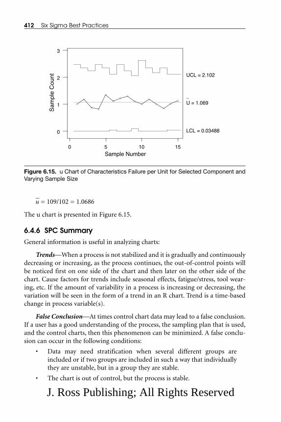
⎯u = 109/102 = 1.0686
The u chart is presented in Figure 6.15.
6.4.6 SPC SummaryGeneral information is useful in analyzing charts:
Trends—When a process is not stabilized and it is gradually and continuouslydecreasing or increasing, as the process continues, the out-of-control points willbe noticed first on one side of the chart and then later on the other side of thechart. Cause factors for trends include seasonal effects, fatigue/stress, tool wear-ing, etc. If the amount of variability in a process is increasing or decreasing, thevariation will be seen in the form of a trend in an R chart. Trend is a time-basedchange in process variable(s).
False Conclusion—At times control chart data may lead to a false conclusion.If a user has a good understanding of the process, the sampling plan that is used,and the control charts, then this phenomenon can be minimized. A false conclu-sion can occur in the following conditions:
• Data may need stratification when several different groups areincluded or if two groups are included in such a way that individuallythey are unstable, but in a group they are stable.
• The chart is out of control, but the process is stable.
412 Six Sigma Best Practices
0 5 10 15
0
1
2
3
Sample Number
Sam
ple
Cou
nt
U = 1.069
UCL = 2.102
LCL = 0.03488
Figure 6.15. u Chart of Characteristics Failure per Unit for Selected Component andVarying Sample Size
J. Ross Publishing; All Rights Reserved

• The chart is in control, but the process is out of control.
Chart Instability—A user is attempting to control a process by constantlyadjusting parameter settings based on past results. Other causes of instabilityinclude:
• Improperly or carelessly setting process parameters
• Automatic control malfunctioning
• Using poor techniques (An R chart may show instability for severalreasons, e.g., using poor logic to define subgroups, using nonrandomsampling, having an improperly trained workforce, etc.)
• Shewhart Control Charts—Generally the control limits set onShewhart charts are ± 3 sigma of the central line. Shewhart controlcharts are considered to be robust due to the 3-sigma limits.
Control charts show various types of nonrandom patterns, e.g., gradualchange, sudden change, staying on one side of the central line for a long time, andsome combination of these situations.
A number of other basic and special control charts are available to resolveissues and help control processes. They all depend on similar logic to determinethe essential decision points that detect out-of-control conditions.
Process—A process need not have a normally distributed variation for con-trol charts to work. Process variation can be predicted only when process varia-tion is known to be in a state of statistical control.
Exercise 6.4: Using SPC Charts
• Identify an opportunity to apply SPC to an input or in-process vari-able as well as to an output in your specific project.
• Determine the type of chart that would be most appropriate for theselected variables.
• Identify:
– Who will be responsible for collecting, charting, and analyzingthe data?
– Does this person have the authority to act in an out-of-controlcondition?
– Are any guidelines in place for troubleshooting an out-of-controlcondition?
Control 413
J. Ross Publishing; All Rights Reserved

6.5 FINAL PROJECT SUMMARY
The structural relationship of the sections discussed in this chapter is presented inFigure 6.1. The activities in Figure 6.1 are control-related activities in the DMAICprocess. Self-control, monitor constraints, error proofing, and SPC have beendetailed and discussed in previous sections of this chapter. The Six Sigma team isnow at a stage when the recommended solution has been implemented and con-trol measures have been installed. The next requirement of the team is to com-plete the final project steps, which include project documentation, implementedprocess instructions, process training, maintenance training, replication opportu-nities, project closure checklist, and identifying opportunities for future projects.
6.5.1 Project Documentation Project documentation is a key step in a Six Sigma project. Format requirementscan vary from business to business, but project documentation is a type of “vir-tual reality” of the process that was followed to accomplish the Six Sigmaimprovements. Project documentation is a permanent record of the project aswell as a guidance tool for others who will be working on a similar type of proj-ect or who plan to continue to work on a recommended project(s) that developedfrom the completed project. Essential elements of project documentation include:
1. State project goals with constraints. State the project goals withapplicable metrics and identifiable constraints:
– Reduce jet engine (model XXXX) manufacturing cycle timefrom 18 months to 14 months: 22% manufacturing cycle timereduction by month/year (XX/XXXX).
– Reduce component and WIP inventory from $XXX to $XXX bymonth/year (XX/XXXX) to provide $XXX in freed-up capital.
– Provide the full opportunity cost of $XXX per year bymonth/year (XX/XXXX).
2. Provide the planned schedule for the project vs. the actual schedule.If the actual schedule is significantly different from the plannedschedule, provide an explanation. An explanation will help futureteams to develop a more-realistic schedule based on availableresources (given constraints).
3. Present the process followed to achieve the project goals. Specifically,identify:
– Tools used to present the information
– How issues were evaluated
414 Six Sigma Best Practices
J. Ross Publishing; All Rights Reserved
– Tools used to develop relationships between independent anddependent variables
– How alternative solutions were developed and then how theimplemented solution was selected.
4. State actual goals achieved.
5. List planned vs. actual achievement of opportunities.
6. State the financial results from the project. Financial results achievedare a most-interesting part of a project. Because the future of a busi-ness depends on the bottom line (profitability), business leadershipis not only interested in the current profitability, but also very highlyinterested in future profitability and growth. Six Sigma projects helpbusinesses to improve profitability. Benefits identified at the begin-ning of the project (during the Define and Measure phases) are gen-erally stated as expected benefits. As the team progresses and goesthrough the Analyze and Improve phases and analyzes the alterna-tive solutions, it has an opportunity to better understand the bene-fits. Once the team recommends a solution to achieve the definedgoals, these benefits are considered to be projected benefits. When theteam implements the recommended solution and collects the sav-ings data, the savings data provide the actual benefits. Benefits datamay change from the beginning of the project (when they areknown as expected benefits) throughout the project to the imple-mentation stage of the project (when they are known as actual ben-efits).
Note: The two sources of financial benefits are cost reduction with the samerevenue and revenue increase with or without any cost adjustments. It is easier tomeasure revenue increase than cost reduction. Cost reduction impacts manyresources, e.g., people, equipment, facility, maintenance of the facility and equip-ment, material, technology, etc. At the beginning of a project, the team analyzesand estimates cost savings and presents them as expected benefits. When the rec-ommended solution has been implemented, team collects benefits data in rela-tionship to the impact of the recommended solution on resources. The team thenpresents this benefits data as actual benefits.
7. Provide “lessons learned” by the project team, e.g., knowledgegained, vital information captured, etc.). Providing lessons learnedapplies to every employee who was directly or indirectly involved inthe project:
– Knowledge gained
– Vital information collected
Control 415
J. Ross Publishing; All Rights Reserved

– How to avoid mistakes
– Necessary activities
Documenting information is crucial. Making information available to othersin the company is also important.
8. Make recommendations for future projects. Because the team is thebest source to recommend future, related projects, the team shoulddocument its recommendations soon after implementing the rec-ommended solution.
9. Provide an instruction manual. As a new or modified process isimplemented, the team must provide a process instruction manual.
General instructions for all types of documentation include:
• The document must be easily accessible. Users should know where thedocument is stored.
• The document must be updated as changes take place. Documentchanges with an effective date.
6.5.2 Implemented Process InstructionsFundamental rules for developing process instructions include the following:
• Simple, precise, and clear instructions must be given.
• Users and responsible process parties must participate in develop-ment of process instructions.
• The text must be limited.
• The instructions must be realistic.
The contents of process instructions should also include, if applicable, the follow-ing, with as many examples as possible:
• Purpose and scope
• CTQs (critical to quality characteristics) parameters to be controlled
• Proper procedures and metrics
• Decision criteria and stages
• Preventive actions to avoid (or minimize) losses
• Corrective actions to minimize losses
• Environmental, health, and safety considerations
• Assumptions (The number of assumptions should be as reasonable aspossible. The assumptions must be tested.)
416 Six Sigma Best Practices
J. Ross Publishing; All Rights Reserved

• Terms and expressions (Definitions and language used will depend onthe users, both professional and/or local.)
• A clear interpretation
• Pictures, flow charts, and tables as appropriate
As a new or modified process is implemented, users of the process must betrained to run as well as maintain the process.
6.5.3 Implemented Process TrainingKey elements in process training include:
• The objectives of the training must be clear and precise.
• Training documents must be prepared before training is started.These documents must meet the same requirements identified inSection 6.5.2, Implemented Process Instructions.
• Communication between students (trainees) and the instructor(trainer) must be good. Students should also have a good knowledgeof the instruction language (reading, writing, understanding, andspeaking).
• The instructor should follow the developed training schedule.Training should be consistent with the material provided.
• Student participation in discussions and hands-on practice duringtraining is very important.
• Keep the students-to-instructor ratio as low as possible.
• As the process changes, supplemental training as needed should beprovided to users.
6.5.4 Maintenance TrainingTwo types of maintenance training are preventive and regular service:
Preventive Maintenance Training—A trainer must demonstrate how:
• To utilize resources in process characteristics that are important tocustomers
• To process maintenance that reduces the chances of system failure
• To replace low-useful-life process components during preventivemaintenance
• To identify process components that need improvement
• To maintain and utilize maintenance data
Control 417
J. Ross Publishing; All Rights Reserved

Regular Service Maintenance Training—Critical points about regular serv-ice maintenance training include:
• The trainer should demonstrate how to repair and replace compo-nents in the process.
• Students should have a good understanding of the process.
• A decision should be made to replace components or to replace ahigher-level process unit.
• The trainer should show how to evaluate process elements forrepair/replacement.
• Maintenance training should demonstrate how to maintain and uti-lize repair data.
• Maintenance should demonstrate how to minimize reactive serviceand develop goals for proactive services.
As the team members develop these documents and provide training to reg-ular users of the process, the team must share its gained knowledge with the othermembers in the business organization. This will provide replication opportunitiesin the business (see the next section).
6.5.5 Replication OpportunitiesThe team should share the information so that other employees in the businesswill have an opportunity to use the knowledge that team members have acquired:
• To avoid wasting resources in solving the same issue
• To speed up the improvement process in the business
• To rapidly resolve issues and improve customer satisfaction
• To reduce DPMO (the defects per million opportunities) at a fasterrate to improve financial benefits
Acquired knowledge can be applied with:
• Direct Replication—By using the same or a similar process for aproduct or service
• Customization—By using same process for different product orservice
• Adaptation—By using the process, but with limited applicability
As the team is engages in the final documentation, training, etc., the teammust ensure that a project closure checklist and a future projects list have beencompleted (see the next two sections).
418 Six Sigma Best Practices
J. Ross Publishing; All Rights Reserved
6.5.6 Project Closure Checklist Developing a project closure checklist is essential. A checklist can easily identifyany leftover activities. Generally, completing a leftover activity is easy for the teamto complete as long as the team is still together. Once the team members are nolonger a defined team, bringing team members together to complete leftoveractivities becomes difficult. Guideline items for a project closure checklist include:
• Project documentation is according to business guidelines.
• Project completion is according to defined goals. Project has beendeclared closed by the project owner.
• The implemented solution has been transferred to regular owners.
• Measurement metrics has been set up to monitor project improve-ments. Then measurement metrics has documented the plan.Improvement will be remeasured at a future (specified) time.
• Financial benefits have been measured. The benefits have beenaccepted by all parties, e.g., project owner, project team, financial,program champion, etc. The savings data collection process has beendocumented.
• Project completion has been identified in the respective databases.
6.5.7 Future Projects The time to examine the collected data and the processes analyzed to determinethe root causes of the issues identified in the project and to identify opportunitiesfor future projects is while the team is still together and memories are still fresh.Questions team members should ask include the following:
• How were key elements in the data identified and verified?
• How did identification of these elements lead to potential causes?
• What was used by the team to make decisions about root causes?
• What was learned and what recommendations were made from:
– A detailed process map
– Data collection, analysis, and identification of root causes
– A project scheduling approach
– A data analysis approach
– Root-cause analysis/cause-and-effect analysis
– Application of qualitative and/or quantitative relationshipsbetween independent variables and the dependent variable
– Financial analysis and data collection
Control 419
J. Ross Publishing; All Rights Reserved

– Project process and procedure
6.6 SUMMARY
In the first five chapters, the first four phases of the DMAIC process (Define,Measure, Analyze, and Improve) have been discussed. Therefore, the processimprovement solution has been selected and implemented and projected benefitshave been realized. The last phase, Control, of the DMAIC process has been dis-cussed in this sixth and final chapter.
Discussion in this chapter has been based on the premise that retaining gainsmade from implementation of the improved/modified process, with the help oftools and techniques (e.g., self-control, monitor constraints, error-proofing, andSPC), are important. Guidance has also been given for developing the final proj-ect summary report. Key elements of a final project summary report include:
• Project Documentation Instructions
• Implemented Process Instructions
• Implemented Process Training
• Maintenance Training
• Replication Opportunities
• Project Closure Checklist
• Future Projects
The following are elements that should be included in a checklist that teammembers should review to ensure that the Control phase of the DMAIC processhas been completed. The elements of the checklist have been divided into keyactivities:
Monitoring Plan
• Has the control/monitoring plan been in place for an adequate periodof time?
• Will the process owner and regular working team members be able tomaintain the gains?
• Have key inputs and outputs been identified to the team members sothat they will be able to measure for and detect suboptimal condi-tions?
• Has adequate training been provided to the owner/team members sothat new or emerging customer needs/requirements will be
420 Six Sigma Best Practices
J. Ross Publishing; All Rights Reserved

checked/communicated to orient the process toward meeting newspecifications and continually reducing variation?
• Has the team been trained in utilizing control charts?
• Do team members know how to calculate their latest Sigma metrics?
• Does established process performance meet customer requirements?
Documented Procedure
• Has proper documentation been developed to successfully supportthe improved operation?
• Have team members been trained and educated about the docu-mented procedures?
• If applicable, have team members been given information about anyrevised work instructions?
• Are developed procedures clear and easy for operators to follow?
Response Plan
• Is a response plan in place so that operators to realize when the input,the process, or the output measures indicate an “out-of-control” con-dition?
• Has a list of critical parameters been developed for operators towatch?
• Have suggested corrective/restorative actions been listed on theresponse plan for the known causes to problems that might surface?
• Has a troubleshooting guide been developed should one be needed?
Project Closure/Transfer of Ownership
• Has process responsibility been transferred to the real owner?Specifically, has it been transferred in the database?
• Has day-to-day process monitoring and continual improvementresponsibility been transferred to the process owner?
• Does the process owner understand how to calculate future Sigmametrics and the process capabilities?
• Has any recommended frequency of auditing been provided to theprocess owner?
• Have any future projects been recommended in a related process?
Control 421
J. Ross Publishing; All Rights Reserved

• Have quality tools been recommended to control process improve-ments?
Project Benefits Linked to the Business
• Has the project closure report recommended other areas of the busi-ness that might benefit from the project team’s improvements, knowl-edge, and lessons learned?
• Has the business been recognizing the best practices and lessonslearned so that improvement can be leveraged across the business?
• Has the business been recognizing that other systems, operations,processes, and infrastructures need updates, additions, changes, ordeletions to facilitate knowledge transfer and improvements, e.g.,activities such as hiring practices, training, employee compensationincluding incentives/rewards, metrics, etc.
Now the team can celebrate their successes and congratulate each other for alltheir hard work!!!
REFERENCES
1. Kumar, D.2003. Lean Manufacturing Systems. Unpublished.
2. Wheeler, D. J. 1995. Advanced Topics in Statistical Process Control: ThePower of Shewhart Charts. Knoxville, TN: SPC Press.
3. Wheeler, D. J. and D. S. Chambers. 1992. Understanding StatisticalProcess Control, Second Edition. Knoxville, TN: SPC Press.
4. Nater, J., W. Wasserman, and M. Kutner. 1990. Applied Linear StatisticalModels: Regression, Analysis of Variance, and Experimental Designs,Third Edition. Chicago: Richard D. Irwin.
* * * *
422 Six Sigma Best Practices
This book has free material available for download from theWeb Added Value™ resource center at www.jrosspub.com
J. Ross Publishing; All Rights Reserved

APPENDICES
Appendix A1. Business Strategic Planning Appendix A2. Manufacturing Strategy and the Supply ChainAppendix A3. Production Systems and Support ServicesAppendix A4. GlossaryAppendix A5. Selected Tables
J. Ross Publishing; All Rights Reserved

J. Ross Publishing; All Rights Reserved

APPENDIX A1 — BUSINESS STRATEGICPLANNING
The rate of return in any business is critical for availability of capital. Investorswill not tolerate returns below the returns of long-term government securities(adjusted upward by the risk of capital loss). Essential structural features of eachindustry determine the strength of competitive forces in that industry and, hence,overall industry profitability. The goal of a competitive strategy for a business unitin any industry is to find a position in the industry in which the company can bestdefend itself against competitive forces or can influence them in its favor. Businessmanagement understands the collective strength of competitive forces, and theresults of competition are apparent. Studying and analyzing underlying sources ofcompetitive forces are essential. Knowledge of the underlying sources of compet-itive pressure will highlight critical strengths and weaknesses of a company.Serious analysis of a company’s position in its industry clarifies areas in which:
• Strategic changes can yield the greatest payoff
• Significant opportunities exist
• Greatest threats exist
Competitive ForcesFive competitive forces are presented in Figure A1.1. A brief discussion will bepresented for:
425J. Ross Publishing; All Rights Reserved
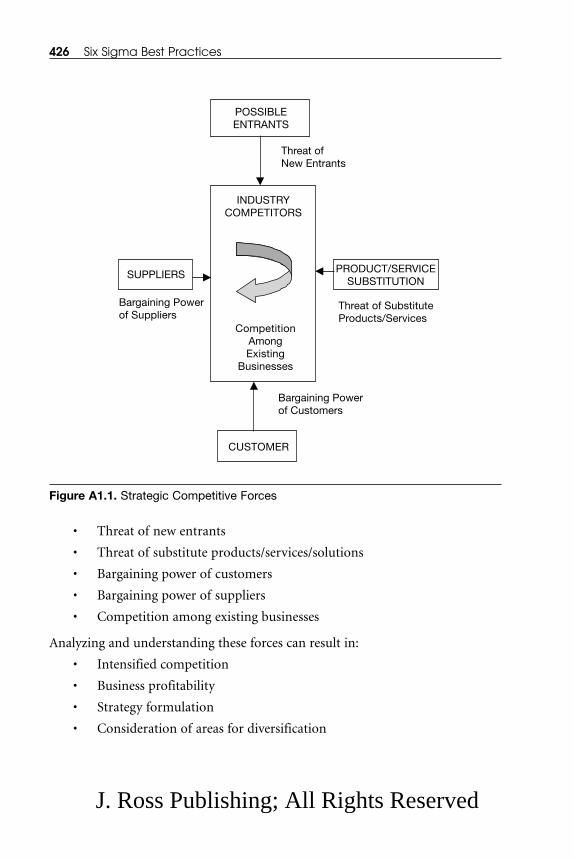
426 Six Sigma Best Practices
• Threat of new entrants
• Threat of substitute products/services/solutions
• Bargaining power of customers
• Bargaining power of suppliers
• Competition among existing businesses
Analyzing and understanding these forces can result in:
• Intensified competition
• Business profitability
• Strategy formulation
• Consideration of areas for diversification
INDUSTRYCOMPETITORS
CompetitionAmongExisting
Businesses
POSSIBLEENTRANTS
PRODUCT/SERVICESUBSTITUTION
CUSTOMER
SUPPLIERS
Threat ofNew Entrants
Bargaining Powerof Customers
Threat of SubstituteProducts/Services
Bargaining Powerof Suppliers
Figure A1.1. Strategic Competitive Forces
J. Ross Publishing; All Rights Reserved

Force 1. Threat of New Entrants—New entrants to an industry bring:
• New capacity
• Desire to gain market share
• Price competition (which generally leads to lower prices that in turnmean consideration of a lower profit margin)
The degree of threat of entry into an industry depends on existing barriers toentry, along with reactions from existing competitors that can be expected by theentrant. If barriers are high and/or a newcomer can expect sharp retaliation fromtough competitors, the threat of entry is low. Several elements reduce incentivesfor new entrants:
• Risk of Capital Investment—Initial capital investment is required inkey business activities, such as product development and production,marketing and sales, research and development, service network, etc.
• Industry Maturity—Because growth potential is generally quite lim-ited, a new entrant will avoid entering a maturing industry.
• Government Policy—A government agency can limit or even force a“closed entry” situation in an industry with controls such as licensingrequirements or by limiting access to raw materials, e.g., land for coalmining, mountains on which skiing areas can be built, etc.
• Regulation—The size of some industries is limited by regulation, e.g.,liquor retailing, railroads, trucking, etc.
• Profit Margin—Generally, new entrants assign low priority to a low-profit-margin business.
• Initial Costs—Initial costs may include the cost to customers ofswitching to another service or product.
• Product Differentiation—Generally established businesses have:- Brand identification- Customer loyalty from past and present products and services- Customer satisfaction
Force 2. Threat of Substitute Products/Services/Solutions—Most businesses inany industry compete by producing substitute products. This limits potentialreturns in the industry due to lower prices. Elasticity of product demand is alsoimpacted. Substitute products that receive the most attention are those that:
• Are subject to having a promising improvement in their price performance compared with the industry’s existing product
• Are produced by industries earning high profits
Appendix A1 — Business Stategic Planning 427
J. Ross Publishing; All Rights Reserved

Force 3. Bargaining Power of Customers—In a competitive market, a customernegotiates lower prices, with on-time delivery, for a quality product and satisfyingservices. This creates significant competition among businesses at the expense ofindustry profitability. The buying power of wholesalers and retailers is deter-mined by the same rules, but retailers get an additional advantage. Retailers cangain significant bargaining power over manufacturers if they can influence thepurchasing decisions of consumers, e.g., as is often true in audio and video com-ponents, personal computer components, sporting goods, etc. Wholesalers cangain similar bargaining power if they can influence the purchasing decisions ofretailers or other firms to which they sell products.
Force 4. Bargaining Power of Suppliers—If there is a limited supply of material(i.e., demand for material is greater than the supply of material), suppliers canexert bargaining pressure over participants in an industry by threatening to raiseprices or lower the quality of existing product and/or services. Supplier groupscan be powerful in certain conditions, e.g., if an industry:
• Is dominated by a few companies and consumers are widely distrib-uted
• Does not produce a substitutable product
• Is not an important customer of a supplier group(s)
• Is a recognized supplier—A workforce must also be recognized as asupplier. Highly skilled employees and/or a tightly unionized work-force can bargain away a significant fraction of potential profits in anyindustry.
Force 5. Competition among Existing Businesses—Competition forces businessesto “jockey” their position within an industry, impacting several elements:
• Price competition
• The advertising battle
• Product modification and/or introduction of new products
• Increased customer service
• Extended warranties
Some form of competition among businesses in any industry is good for con-sumers as well as for the industry. Yet, price competition can sometimes make anindustry highly unstable, likely leaving the entire industry worse off from a stand-point of profitability. Price cuts are quickly and easily matched by rivals, and oncematched, price cuts lower revenues for all businesses unless the price elasticity ofdemand in the industry is high.
428 Six Sigma Best Practices
J. Ross Publishing; All Rights Reserved

Advertising battles, on the other hand, may well expand demand or enhancethe level of product differentiation in the industry to the benefit of all businesses.Intense competition is a result of several factors:
• Numerous or Equally Balanced Competitors—When businesses arenumerous in any industry, some businesses may think that they canmake “moves” without being noticed.
• Slow-Growth Industries—Some businesses want to gain market sharein a slow-growth industry, which in turn creates intense competition.
• High Fixed or Storage Costs—When excess capacity is available, busi-nesses are forced to produce more and sell more, which often leads torapidly escalating price cutting, e.g., as in the aluminum and paperindustries.
• Lack of Differentiation—Similar services or switching costs mayspark competition, e.g., low-cost services.
• High Strategic Stakes—Competition in any industry becomes evenmore intense if a number of businesses have high stakes in achievingsuccess, e.g., Sony or Philips might perceive a strong need to establisha solid position in the U.S. market to build global prestige or techno-logical credibility.
• High Exit Barriers—Exit barriers are economic, strategic, and emo-tional factors that keep companies competing in an industry even ifthey are earning low revenues or losing money. Major barriers to exit-ing an industry include:
– Specialized assets
– High fixed costs of exit
– Emotional barriers
– Government and social restrictions
StrategiesAs businesses cope with the five competitive forces, three potentially successfulgeneric strategic approaches can result in some businesses outperforming otherbusinesses in a respective industry:
• Overall cost leadership
• Differentiation
• Focus
Sometimes a business can successfully pursue more than one approach as itsmain target, although this is rarely possible. Effectively implementing any of the
Appendix A1 — Business Stategic Planning 429
J. Ross Publishing; All Rights Reserved

generic strategies generally requires strong commitment and supportive organi-zational arrangements. Organizational commitment and support are oftendiluted by having more than one primary target.
Strategy 1. Overall Cost Leadership—Lowest-cost-producer leadership requiresimplementation of at least:
• Efficient-scale facilities
• Vigorous leadership of cost reduction from experience and from tightcost and overhead control
• Minimizing marginal customer accounts
• Cost minimization in areas, e.g., research and development, service,sales, advertising, etc.
A low-cost-producer position in any business generally yields above-averagereturns in the industry despite the presence of strong competitive forces. A low-cost position:
• Defends a business against buyers—Buyers can exert pressure, drivingprices down to the level of the next most-efficient competitor.
• Provides a defense against powerful suppliers by providing more flex-ibility to cope with input cost increases
• Provides entry barriers in terms of economies of scale or cost advantages
• Usually places a business in a favorable position as well as utilizes aproduct substitute that is relative to its competitors in the industry
A cost leadership strategy can sometimes revolutionize an industry in whichthe historical bases of competition have been to use other methods or in whichcompetitors are not prepared perceptually or economically to take the necessarysteps for cost minimization, e.g., low-cost Southwest Airlines in competition withother airlines such as American, Delta, etc.
Strategy 2. Providing Differentiation—Offering products or services that are per-ceived industry-wide as unique is a viable strategy for earning above-averagereturns in an industry because a defensible position, different from cost leader-ship, is created for coping with the five competitive forces. Differentiationapproaches include:
• Design or brand image• Technology• Features• Customer service• A dealer network
430 Six Sigma Best Practices
J. Ross Publishing; All Rights Reserved

Strategy 3. Focus—Focusing on a particular customer group, a segment of theproduct line, or a geographic market is similar to differentiation and can takemany forms. Low-cost and differentiation strategies are aimed at achieving objec-tives industry-wide, but the focus of a strategy is built around serving a particu-lar target very well. Each functional policy is developed with this goal in mind. Abusiness achieving focus can potentially earn above-average returns in its indus-try. Focus indicates that a business either has a low-cost position compared to itsstrategic target, high differentiation, or both.
RisksEach strategy has risks:
• Risks of Generic Strategies—Two risks are linked to generic strategies:
– Failing to attain or sustain a strategy
– A strategic advantage that is not strong enough to compensate forlosses due to industry evolution
• Risks of Overall Cost Leadership—Cost leadership imposes severeburdens on a business to maintain its position, e.g., reinvesting inupgraded machines (systems), ruthlessly scraping obsolete assets,controlling product line proliferation, and being alert to technologi-cal improvements.
• Risk of Differentiation—Risks involved with differentiation include:
– The cost differential between low-cost competitors and the differ-entiated business may become too great for differentiation tomaintain brand loyalty. Therefore, customers sacrifice some ofthe features, services, or the image of the differentiated businessfor larger cost savings.
– As customers become more sophisticated, they require differenti-ating factors less.
– Often, as an industry matures, imitation narrows perceived dif-ferentiation.
• Risk of Focus—Focus includes another set of risks:
– The cost differential between broad-range competitors and afocused business widens to eliminate the cost advantages fromserving a narrow target or they offset the differentiation achievedfrom focusing.
– Differences between a strategic target and the market as a wholenarrow for desired products or services.
– Competitors find submarkets within the strategic target and “outfocus” a focused business.
Appendix A1 — Business Stategic Planning 431
J. Ross Publishing; All Rights Reserved

Detailed Strategic PlanningAn introductory analysis of business strategy has been described, but a more-detailed study of strategic business planning would include three steps:
Step 1. Along with introductory analysis, add:
• Analyzing competitors, customers, and suppliers
• Understanding the techniques of reading market signals
• Analyzing theoretic concepts for making and responding to competi-tive moves
• Developing an approach to mapping strategic groups in the industryand explaining differences in their performance
• Defining a framework for predicting industry evolution
Step 2. Utilize the introductory framework:
• Develop a competitive strategy for the environment in a particulartype of industry.
• Identify possibilities for differentiation. Differentiating environmentsis crucial in determining the strategic context in which a businesscompetes, the strategic alternatives available, and common strategicerrors.
Step 3. Identify strategic areas by:• Examining and categorizing the business:
– Fragmented industries
– Emerging industries
– Industries in transition to industry maturity
– Declining industries
– Global industries
• Systematically examining the important types of strategic decisionsthat confront businesses competing in a single industry
• Utilizing other essential activities, e.g., vertical integration, capacityexpansion, and entry into a new business.
• Determining if corporate strategies for marketing, manufacturing,and distribution are a “fit”—Strategies must fit together to meet cus-tomer needs at minimum cost. Possible alternatives include:
– Concentrating on marketing, with total manufacturing and dis-tribution being subcontracted to outside suppliers
432 Six Sigma Best Practices
J. Ross Publishing; All Rights Reserved

– Concentrating on manufacturing activities, with sales and adver-tising being contracted out
ADDITIONAL READING
1. Kumar, D. 2003. Lean Manufacturing Systems. Unpublished.
Appendix A1 — Business Stategic Planning 433
J. Ross Publishing; All Rights Reserved

J. Ross Publishing; All Rights Reserved

APPENDIX A2 —MANUFACTURING STRATEGY AND THE SUPPLY CHAIN
Manufacturing strategy and the supply chain are interdependent topics, thereforean overview is required to describe these topics.
Manufacturing Strategy1
If strategic planning activities have not been properly performed, knowing if abusiness is moving in the right direction (or not) will be difficult. A strategic busi-ness plan provides a view of the business (with direction) and provides a roadmap showing the direction the business should take to achieve its goals.
The desired marketplace position of a business to satisfy its customers isstated in a general way in a strategic plan. A strategic plan should also include tar-gets for market share, sales, quality, on-time delivery, inventory level, profitability,etc. A strategic plan leads to a strategic manufacturing plan. A strategic manufac-turing plan identifies products to be produced, production technology that will beused to produce the products selected, and manufacturing policies that will be fol-lowed for purchasing, manufacturing, and distribution.
Certain essential elements impact any manufacturing strategy:
• Location of manufacturing facilities
• Product distribution network
435J. Ross Publishing; All Rights Reserved

• Inventory policies that are matched to selected geographical marketsand the required speed of delivery
• Policies that are related to the employment level of a knowledgeableworkforce, with employee training and benefits
• Core competencies
• Vertical integration
• Supporting decisions
– Make vs. buy
– Make-to-stock vs. make-to-order
– Selection of technology and equipment
The Supply Chain Natural raw material goes through a series of processes to produce an ultimatecustomer product. One or more manufacturers might participate in the process.The planning and execution of these processes comprise the logistics function.The logistics function illustrates the entire supply chain from raw materials todelivered product. Key elements of an effective logistics function include:
• The functional capability of all potential suppliers and their geo-graphical locations
• Manufacturing facilities at a business
• Customer markets
• Transportation sources that connect supplier, manufacturer, and cus-tomer
The most competitive option is selected from these resources with respect tothe product, the cost of the product, quality, on-time availability to customers,and after-delivery service to customers. The logistics function creates a networkknown as a logistics network. Information management in a logistics network iscritical. Twenty-first century logistics or global logistics describes a modern globalmarket.2
Global Logistics—The peacetime economy after World War II slowly movedtoward globalization, but accelerated at a fast pace at the beginning of the twenty-first century. Businesses were creating global production and distribution net-works to take advantage of international opportunities.
In the current global economy, businesses often design, manufacture, and dis-tribute products through a global network to provide the best customer service ata competitive price. Businesses are making a profit margin even with the interna-tional challenges of diverse cultures, languages, people, governmental regulations,
436 Six Sigma Best Practices
J. Ross Publishing; All Rights Reserved

and measurement systems because conditions are positive for international busi-ness, e.g., instantaneous information exchange, improved transportation, etc.
Often, a significant number of products reflect multinational business ven-tures. Mixing of components in finished products has also become commonplace,e.g., the automobile industry and its utilization of this concept. Participating busi-nesses also benefit by sharing technology and the market.
Other essential elements in supply chain management include:
• Product design and customization to the local market
• Supplier selection, certification, and long-term contracts
• Distribution of finished components and products
• Locating and distributing inventory
Coordinating production schedule information across the supply chain isimportant. Without proper communication and planning coordination, variationat the final-customer end of the supply chain can accelerate upstream in a chaoticmanner. According to Askin and Goldberg,2 this phenomenon is referred as the“bullwhip effect.”
Manufacturing strategy has a critical role in any company’s decision to selecta supply chain process. Therefore, a strategic plan must consider facilities,processes, people, and products in developing a purchasing, manufacturing, dis-tribution, and service plan.
REFERENCES
1. Kumar, D. 2003. Lean Manufacturing Systems. Unpublished.
2. Askin, R.G. and J.B. Goldberg. 2002. Design and Analysis of LeanProduction System. New York: John Wiley.
Appendix A2 — Manufacturing Strategy and the Supply Chain 437
J. Ross Publishing; All Rights Reserved

J. Ross Publishing; All Rights Reserved

APPENDIX A3 —PRODUCTION SYSTEMS AND SUPPORT SERVICES
Production Planning and Support Services DecisionsProduction planning and support services decisions are typically made in a hier-archical manner1 as shown in Figure A3.1. The first column in the figure showsthe actual flow of material from raw stage through delivered product/solution.Twenty-first century suppliers deliver solutions to customers. A solution could bea combination of hardware, software, and professional services.
The last column in Figure A3.1 shows associated support functions anddesign activities that must be available before the start of production and supportservices activities for customers. The middle column shows the sequence of oper-ational decisions for production planning, scheduling, and control. These deci-sions are listed in the hierarchical order in which they usually are made.
The level of professional services depends on customer requirements.Professional services may be required before system delivery, during system deliv-ery, and/or during the system’s useful life. Demand forecasts define the opportu-nity to make profits and have gainful employment by providing satisfaction tocustomers.
The Decision ProcessThe decision process2 is hierarchical in a production system. Figure A3.2 summa-rizes the manufacturing system in an IPO (Input-Process-Output) format.
J. Ross Publishing; All Rights Reserved

440 Six Sigma Best Practices
TechnicalSupportServices,
ProfessionalServices
Product Distribution
Customer
Marketing and Sales
FinishedProduct
Hardwareand/or
Software
AdministrativeFunctions, e.g.,
Purchasing,Financial,
Human Resources, Safety and Security
Product DesignTest Engineering
Process Engineering
ManufacturingSupport, e.g.,
FacilitiesPlanning, Tooling Support, Product
Reliability,Maintainability,
andQuality Control
Product Flow
Product ProductionPlanning and Decision
Hierarchy
Technical and Administrative
Support Services
Forecasting
StrategicPlanning
AggregateProductionPlanning
DetailedPlanning
ProductionScheduling:High-Levelto DetailedScheduling
Shop FloorControl
MaterialSupplier(s)
ComponentManufacturing
Product/System
Assembly and
Integration
Figure A3.1. Production Planning and Support Services Information Flow Chart
J. Ross Publishing; All Rights Reserved

Appendix A3 — Production Systems and Support Services 441
StrategicPlanning
AggregateProductionPlanning
DetailedPlanning
ProductionScheduling
ProductionControl
Inputs Process OutputsPlanningHorizon
Technical Support
Services/ Professional
Services
Operating Facilities Product Families Technologies
Production Level Workforce Level Product Family Inventories
Master: Production Schedule Component Inventory
Work Center: Schedules Order Releases Job Priorities
Work Center: Priorities Job Status Workforce Reporting Material Handling and TrackingJob Unloading
Provide Services to Maintain Customer System in Available Condition
Years
Months
Weeks
Daily
Real-Time Basis
Real-Time Basis
Long-Range Economic Forecast Capital Availability Feedback Loop
Processing Technology Medium-Range ForecastProduct Families Work Center Schedules
Production Levels Workforce Levels Inventory Status Job Setup Data Product Forecast
Master Production ScheduleBill of Materials Process Plans
Workforce Status Manufacturing System Status Job Priority Manufacturing Order ReleasesWork Center Schedules
Customer Expectations/ Requirements
Figure A3.2. Inputs, Processes, and Outputs in a Manufacturing System
J. Ross Publishing; All Rights Reserved

Decisions are made at several levels in all businesses. These decisions are generallytime-based and, therefore, highly dependent on the type of business:
• Strategic Level—Long-term decisions are at the strategic level and arenormally for a 1- to 5-year time frame, but the time frame can belonger in certain industries. Making a capital investment is an exam-ple of a strategic-level decision, e.g., an investment in facilities, equip-ment, tools, etc.
• Tactical Level—A decision at the tactical level is a shorter-term deci-sion (e.g., monthly, quarterly, etc.) to implement strategic-level deci-sions, e.g., aggregate production planning in a manufacturing area. Atypical manufacturing aggregate plan states the levels of major prod-uct “families” that are to be produced monthly over the next 12months or so. Examples of other tactical level manufacturing deci-sions include:
– Change in workforce level
– Scheduling overtime
– Built-in inventory
• Operational Level—Decisions at the operational level are made on adaily or weekly level, e.g., detailed scheduling at a component andassembly level to meet a customer’s requirements. Most customerservice decisions fall in this category, especially after product (system)delivery. For customers, on-time service delivery is as critical as deliv-ery of the product.
A hierarchical organizational structure supports production decisions. Thesize of the organization depends on the type of product (system). A short-lifeproduct has a “flatter” production organizational structure than a long-life prod-uct. In a complex system, making group decisions for all decisions in a plant/pro-duction facility, and also making them in real time, is almost impossible due to thecomplexity of the entire system.
REFERENCES
1. Kumar, D. 2003. Lean Manufacturing Systems. Unpublished.
2. Askin, R.G. and J.B. Goldberg. 2002. Design and Analysis of LeanProduction System. New York: John Wiley.
442 Six Sigma Best Practices
J. Ross Publishing; All Rights Reserved

A
Accuracy.The degree to which a measurementsystem is accurate will generally be thedifference between an observed aver-age measurement and the associatedknown standard value.
Alternate Hypothesis.The second hypothesis is known as thealternate hypothesis. It is symbolizedby H1.
BBalanced Design.A balanced experimental design is adesign in which each level for any onefactor is repeated the same number oftimes for all possible combination lev-els of the other factors, e.g., a factorial
design of two factors (A and B) andtwo levels (–1, 1) will have four runs.
Binomial Distribution.This distribution is used when a possi-bility of an occurrence of one of thetwo possible outcomes exists in everytrial (e.g., accept or reject; success orfailure) and the probability for eachtrial remains constant. This distribu-tion is also known as Bernoulli’s distri-bution.
Black Belt (BB) Certified.A Black Belt-certified person shouldhave sufficient knowledge and techni-cal training to achieve project goals.Black Belt training includes problemsolving and improvement skills, quan-tifying project savings, project man-agement skills, project reporting skills,and training in the statistical tools
443
APPENDIX A4 — GLOSSARY
J. Ross Publishing; All Rights Reserved

required to measure, analyze, improve,and control a project.
Box Plot.Box plots are similar to histograms.They provide a graphic summary ofthe variation in a given set of data with“whiskers” and “outliers.” A Box Plotgroups data points into four main cat-egories known as quartiles. A Box Plotis an excellent tool for comparing sam-ples of data.
CCapability.The ability of a process to produce aproduct/service within defined specifi-cation limits is known as capability.
Census.If all data on a population are col-lected, census is another descriptiveterm that can be used.
Chi-square Distribution (χ2 Distribution).A χ2 distribution is specific type ofsampling distribution that is known aschi-square or χ2.
Coefficient of Correlation (√r2 = r).The square root of the sample coeffi-cient of determination is a commonalternative index of the degree of asso-ciation between two quantitative vari-ables.
Coefficient of Determination (r2).How well the estimated regression linefits the sample data, or the amount ofvariation explained by the regression
equation, is measured by the coeffi-cient of determination (r2).
Common Cause.A common cause is due to inherentinteraction among input resources. Itis normally expected, random, andpredictable.
Confidence Interval.A confidence interval is an interval thathas a designated chance of includingthe universal value.
Confidence Limits.The end points of a confidence intervalare the confidence limits.
Consumer’s Risk (Type II Error or β).Accepting a hypothesis when it is nottrue, i.e., a type II error has been made(e.g., accepting bad parts as good), isknown as consumer’s risk. β is the riskof not finding a difference when thereactually is one. See also Producer’sRisk.
Control Charts.Control charts are graphical devicesthat highlight the average performanceof a data series and the dispersionaround the average. Control charts arean important tool in statistical processcontrol.
Critical to Quality Characteristics(CTQs).Key measurable characteristics ofproduct/process/service performancestandards that must be met to satisfyan external (ultimate) customer areknow as CTQs. From the customer’s
444 Six Sigma Best Practices
J. Ross Publishing; All Rights Reserved

point of view, to be a satisfied cus-tomer, CTQs are the “vital few” meas-urable characteristics of a product or aprocess in which performance stan-dards must be met.
Customer.Customer defines a product and/orservice requirement that is delivered bya manufacturer and/or supplier.Consumer may also be defined as anindividual or organization thatreceives the processed output.
DDefect.A defect is anything that prevents abusiness from serving its customers asthey prefer to be served.
Dependent Variable.The value of the dependent variable isassumed to be unknown and is sym-bolized by Y. This variable is oftencalled the response variable.
Design of Experiment (DOE).DOE is an acronym that identifies howfactors (independent variables, Xs),individually and in combination, affecta process and its output (dependentvariables, Ys). DOE develops a mathe-matical relationship and determinesthe best configuration or combinationof independent variables, Xs.
DFSS .DFSS is an acronym for design for SixSigma. See DMADV methodology.
DMADV Methodology (Duh-may-dove).DMADV is an acronym for a five-phase process—Define, Measure,Analyze, Design, and Verify. DMADVis a scientific closed-loop process thatis systematic and relies on the use ofstatistics. It applies to a product orprocess that is not in existence at abusiness and needs to be developed.
DMAIC Methodology (Duh-may-ik).DMAIC is another acronym for a five-phase process—Define, Measure,Analyze, Improve, and Control.DMAIC is a scientific closed-loopprocess that is systematic and relies onthe use of statistics. It is a popular SixSigma process. Existing products orprocesses are optimized using theDMAIC process.
DPMO.DPMO is an acronym for defects permillion opportunities. See PPM.
EEffectiveness of Measures.Effectiveness of measures indicatesmeeting and exceeding customer needsand requirements, e.g., in areas such asservice response time, percent productdefective, and product functionality.
Efficiency of Measures.Meeting and exceeding customerrequirements based on the amount ofthe resources allocated is known asefficiency of measures, e.g., productrework time, product cost, and activitytime.
Appendix A4 — Glossary 445
J. Ross Publishing; All Rights Reserved

EPMO.The acronym EMPO, or the errors permillion opportunities, is a metric formeasuring and comparing the per-formance of distinct administrative,service, or transactional processes.EPMO quantifies the total number oferrors or mistakes produced by aprocess per million iterations of theprocess.
Experiment, in Six Sigma.In a Six Sigma context, an experimentis a planned inquiry, to obtain newfacts or to confirm or deny the resultsof previous experiments, in which theinquiry is made to aid a team in a deci-sion-making process.
Exponential Distribution.Exponential distribution representsactivity performance time. This distri-bution is closely related to the Poissondistribution, e.g., if customer arrival atthe bank has a Poisson distribution,customer service time at the bankwould have an exponential distribu-tion.
FFactor.A factor is an input in an experiment.It could be a controlled or uncon-trolled variable whose impact on aresponse is being studied in an experi-ment. The factor could be qualitative,e.g., different operators, machinetypes, etc., or it could be quantitative,e.g., distance in feet or miles, time inminutes, etc.
Factorial k1 × k2 × k3 … This is a basic description of a factorialexperiment design. Each k represents afactor. The value of k is the number oflevels of interest for that factor, e.g,a 3 × 2 × 2 design indicates that thereare three input variables (factors). Oneinput has three levels and the other twohave two levels each.
FMEA.FMEA is an acronym for failure modeand effects analysis.
FMECA.FMECA is an acronym for failure,mode, effects, and criticality analysis.
Flow Chart.A flow chart is a pictorial representa-tion of a process where all the steps ofthe process are presented. A flow chartis also a planning and analysis tool. It isa graphic of the steps in a workprocess. A flow chart is also a formal-ized graphic representation of a workor process, a programming logicsequence, or a similar formalized pro-cedure.
GGamma Distribution.The gamma distribution takes differ-ent shapes as the value of the shapeparameter (r) changes. When r = 1, agamma distribution reduces to anexponential distribution.
Green Belt (GB) Certified.A Green Belt-certified person should betrained to support/participate in aChampion’s Six Sigma implementation
446 Six Sigma Best Practices
J. Ross Publishing; All Rights Reserved

program. A GB should also be able tolead a small Six Sigma project. A GBtraining program provides a thoroughunderstanding of Six Sigma and theSix Sigma focus on eliminating defectsthrough fundamental process knowl-edge. GB-certified employees are alsotrained to integrate the principles ofbusiness, statistics, and engineering toachieve tangible benefits.
HHistogram.A histogram is a bar diagram repre-senting a frequency distribution.
Hypothesis.A hypothesis is an intial proposition(for the time being) that is recognizedas possibly being true.
Hypothesis Testing.Hypothesis testing is a systematicapproach for assessing an initial belief(a hypothesis) about reality. It con-fronts the belief with evidence andthen decides, in light of this evidence,if the initial belief/hypothesis can bemaintained as “reasonable” or if itmust be discarded as “untenable.”
IIndependent Variable.The value of a variable assumed to beknown is symbolized by X and knownas the independent variable.
Input.Resources (equipment, facility, mate-rial, people, technology, and utilities)and the data that is required to execute
a process (operation) are known asinput.
LLevel(s).The input values of a factor beingstudied in an experiment are known aslevels. Levels should be set far enoughapart so that effects on the dependentvariable Y can be detected. Levels aregenerally referred to as “–1” and “1.” Alevel is also known as a treatment.
LCL.LCL is an acronym for lower controllimit. The LCL is equal to (μ – nσ) forpopulation and (Xbar – ns) for sample.
LSL.LSL is an acronym for lower specifica-tion limit.
MMaster Black Belt (MBB, also Master).MBBs are generally program-site tech-nical experts in Six Sigma methodol-ogy. MBBs are responsible forproviding technical guidance to teamleaders and members. Most of thetime, MBBs are dedicated full time tosupport a program. They are to be anexpert resource for their teams, e.g., forcoaching, statistical analysis, and Just-In-Time training. Masters, along withteam leaders, determine the team char-ter, goals, and team members. Theyalso formalize studies and projects. AMaster can support up to ten projects.
Appendix A4 — Glossary 447
J. Ross Publishing; All Rights Reserved

Method of Least Squares.Fitting the data to a line in a scatterdiagram is known as the method ofleast squares. The line is developed sothat the sum of the squares of the ver-tical deviations between the line andthe individual data plots is minimized.
MINITAB®.MINITAB® is a statistical softwarepackage with high-quality, exportablegraphics. Input data can be trans-ported directly from an Excel™spreadsheet. Recognizing the differ-ence between text data and numericdata is important when usingMINITAB.
NNID(0, σ2).For hypothesis testing, model errorsare assumed to be normally and inde-pendently distributed random vari-ables with a mean of zero and avariance of σ2 [abbreviated as NID(0,σ2)]. The variance σ2 is assumed con-stant for all levels of the factor.
Nominal Group Technique.A structured process which identifiesand ranks the major problems or issuesthat need addressing is known as anominal group technique.
Non-Value-Added Activity.Activity that a customer is not inter-ested in and for which a customer isnot willing to pay is known as non-value-added activity. Manufacturers/suppliers need non-value-added activ-ity to support their businesses.
Normal Data (Common LanguageCommunication).A frequency distribution of normaldata appears to cluster around an aver-age (mean) and trails off symmetri-cally in both directions from the mean.A graph of the frequency distributionof normal data forms the shape of abell (known as a bell curve). In statis-tical terms, this type of distribution isknown as a normal distribution or aGaussian distribution. A standard nor-mal distribution has a mean of zeroand a standard deviation of 1.
Null Hypothesis.The first hypothesis in a set is knownas a null hypothesis. It is symbolized byH0.
OOne-Sided Hypothesis.An alternate hypothesis that holds fordeviations from the null hypothesis inone direction only is known as a one-sided hypothesis.
Outlier.Any data point (usually consideredanomalous), which is well beyondexpectations, is known as an outlier. Ina Box Plot, outliers are displayed asasterisks (*) beyond the “whiskers.” Seealso Box Plot.
Output.Output is a tangible product or servicethat is the result of a process to meetcustomer demand.
448 Six Sigma Best Practices
J. Ross Publishing; All Rights Reserved

PPareto Chart.A bar graph of counted data is knownas a Pareto chart. The frequency ofeach category is displayed on the Y-axis(vertical axis). Category type is dis-played on the X-axis. Frequency dataare arranged in descending order.
Poisson Distribution.The Poisson distribution estimates theoccurrence of a number of events thatare of the same type during a definedperiod.
PPM.PPM is an acronym for parts per mil-lion or the number of defects in a pop-ulation of a sample of one million(1,000,000). See DPMO.
Process.A process is one or more operationsthat is performed over the input(s) andthat change(s) the input into an outputto meet a customer’s demand.
Process Boundary.The limits of a particular process areknown as the process boundary (usu-ally identified by the inputs and out-puts which are outside the processboundary).
Process Capability Index (Cpk).Cpk measures the ability of a process tocreate a product within specificationlimits.
Process Potential Index (Cp).Cp measures the potential capability ofa process. Cp is defined as the ratio of
the allowable spread over the actualspread.
Producer’s Risk (Type I Error or α).To reject a hypothesis when it is actu-ally true is known as producer’s risk,e.g., rejecting good parts as being badparts. α is the risk of finding a differ-ence when there actually is a differ-ence. See also Consumer’s Risk.
RRandomness.Data should be collected in no prede-termined order. Therefore, each ele-ment will have an equal probability tobe selected for measurement.
Reengineering.Reengineering is a process in whichunnecessary tasks are eliminated, taskscan be combined or reordered, andinformation can be shared among theentire workforce involved in a process,etc.
Regression Analysis.A statistical method, with a key focuson establishing an equation that allowsthe unknown value of one variable tobe estimated from the known value ofone or more other variables, is knownas regression analysis.
Regression Equation.A prediction equation, which can belinear or curvilinear, allows theunknown value of one variable to beestimated from the known value ofone or more other variables.
Appendix A4 — Glossary 449
J. Ross Publishing; All Rights Reserved

Regression Line.In regression analysis, a line that sum-marizes the relationship between anindependent variable, X, and adependent variable, Y, while also mini-mizing the errors made when theequation of that line is developed toestimate Y from X, is known as theregression line.
Repeatability.If data being collected (measured) arerepeatable, this condition is known asrepeatability.
Repetition.Running more than one experimentconsecutively, and using the sametreatment combinations, is known asrepetition.
Replication.Using the same experimental setup,with no change in the treatment levels,more than once, to collect more thanone data point is known as replication.Replicating an experiment would allowa user to estimate the residual or theexperimental error.
Reproducibility.If all data collectors are observing thesame activity and measuring the timefor an activity with the same equip-ment, they should all reach essentiallythe same outcome.
Response Variable. See DependentVariable.
Root Cause.The lowest-level basic cause of a vari-ance is known as the root cause.
SSampling.Sampling is a portion or subset of thetotal data collection process.
Sigma.Sigma is a symbol for the standarddeviation of a process mean on eitherside of the specification limit.
Significance Level.All sample results, which are possiblewhen a null hypothesis is true, areknown as the significance level. It is the(arbitrary) maximum proportion thatis considered sufficiently unusual toreject a null hypothesis.
Simple Correlation Analysis.A key focus of this statistical method isestablishment of an index that pro-vides, in a single number, an instantmeasure of the strength of associationbetween two variables. Depending onthe value of this measure (0 to 1), onecan tell how closely together two vari-ables move and, therefore, how confi-dently one variable can be estimatedwith the help of the other.
Simple Regression Analysis.When a single variable is used to esti-mate the value of an unknown vari-able, the method is known as simpleregression analysis.
450 Six Sigma Best Practices
J. Ross Publishing; All Rights Reserved

SIPOC (Sy-pock).SIPOC is an acronym for a process ofsteps in high level-business mapping,where S = supplier, I = input from sup-plier, P = business performed process,O = process output, and C = customer(internal and external). Supplier(s)provide input(s). A business performsone or more operations on theinput(s) to produce an output to meeta customer’s demand.
Six Sigma, the Statistical Term.In pure statistical terms, Six Sigma is0.002 defect per million parts, or 2defects per billion parts, or a yield99.9999998%.
Six Sigma, the Motorola Terminology.In Motorola terminology, Six Sigma isa process, a metric, a statistic, a value, avision, or a philosophy, depending onthe context being discussed. It is aprocess that is focused on excellence.Six Sigma reduces the variance in anyparameter that a customer deems crit-ical to quality. It is a defect rate of notmore than 3.4 parts per million, whichallows a ± 1.5 sigma (long-term) shiftfrom the statistical value (3.4 PPM isonly ± 4.5 σ on the statistical scale).
Special Cause.An especially large influence by one ofthe input resources is known as a spe-cial cause. A special cause is generallyunpredictable or abnormal.
Stakeholders.Stakeholders sponsor a project. A proj-ect team periodically reports project
status to stakeholders. Stakeholdersimpact a process or a process impactsthem.
Standard Deviation (SD).The square root of the average of thesquared deviations from the mean isknown as the standard deviation.Standard deviation is designated by thesymbol σ for population and by thesymbol s for sample. Standard devia-tion is also a commonly used measureof the general variability of the datafrom the mean.
Statistic.A function of sample observations thatis used to estimate a universe parame-ter is known as a statistic.
Statistical Hypothesis.A statistical hypothesis is a statementabout the probability distribution of arandom variable, e.g., interest may bein determining the mean tensilestrength of a particular type of steel,i.e., specifically, the interest is in decid-ing whether or not the mean tensilestrength is 15,000 psi.
Statistical Process Control (SPC).An SPC is a problem-solving tool thatmay be applied to any process. SeveralSPC tools are available. SPC is also adesire by all individuals in abusiness/product/process group forcontinuous improvement in qualitythrough the systematic reduction ofvariability.
Appendix A4 — Glossary 451
J. Ross Publishing; All Rights Reserved

Stratification.Stratification is the process of separat-ing data into categories (or groups)based on data variation.
Student’s Distribution. See t Distribution.The t distribution is also known asStudent’s distribution.
Supplier.A supplier is source that provides inputto a business process.
Tt Distribution. See Student’sDistribution.A t distribution is particular type ofsample distribution. It is also known asStudent’s distribution.
Total Sum of Squares (TSS).TSS is the sum of the squares of thedeviations of individual items from themeans of all the data.
Treatment Combination.Identifying the experiment runs, usinga set of specific levels for each inputvariable, is known as treatment combi-nation. A full experiment uses all treat-ment combinations for all factors, e.g.,a 3 × 2 × 2 factorial experimentaldesign will have 12 possible treatmentcombinations in the experiment.
Two-Sided Hypothesis.An alternate hypothesis that holds (istrue) for deviations from the nullhypothesis in both directions is knownas a two-sided hypothesis.
Type I Error.See Producer’s Risk or α.
Type II Error.See Consumer’s Risk or β.
UUnbalanced Design.A designed experiment that is notmeeting the criteria of a balanceddesign is known as unbalanced design.An unbalanced design is also a designin which each experimental level forany one factor is not repeated the samenumber of times for all possible levelsof the other factors.
UCL.UCL is an acronym for the upper con-trol limit. UCL is equal to (μ + nσ) forpopulation and ( ⎯X + ns) for sample.
USL.USL is an acronym for the upper spec-ification limit.
VValue-Added Activity.An activity for which a customer iswilling to pay and to support is knownas value-added activity.
Variance.The square of the standard deviation isknown as variance.
W
Waste.An activity that does not supporteither a customer or a manufacturer
452 Six Sigma Best Practices
J. Ross Publishing; All Rights Reserved
/supplier and for which no one is will-ing to pay is known as waste.
Weibull Distribution.This distribution provides an excellentapproximation of the probability lawof many random variables. An impor-tant area of the Weibull distributionapplication is as a model for the time-
to-failure in electrical and mechanicalproducts and systems.
ZZ Value.Any value away from the mean ismeasured in terms of standard devia-tion. Z is a unit of measure that isequivalent to the number of standarddeviations.
Appendix A4 — Glossary 453
J. Ross Publishing; All Rights Reserved

J. Ross Publishing; All Rights Reserved

APPENDIX A5 —SELECTED TABLES
455J. Ross Publishing; All Rights Reserved
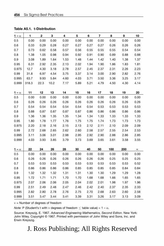
456 Six Sigma Best Practices
Table A5.1. t-Distribution
1 – α 1 2 3 4 5 6 7 8 9 10
0.5 0.00 0.00 0.00 0.00 0.00 0.00 0.00 0.00 0.00 0.00
0.6 0.33 0.29 0.28 0.27 0.27 0.27 0.27 0.26 0.26 0.26
0.7 0.73 0.62 0.58 0.57 0.56 0.55 0.55 0.55 0.54 0.54
0.8 1.38 1.05 0.98 0.94 0.92 0.91 0.90 0.89 0.88 0.88
0.9 3.08 1.89 1.64 1.53 1.48 1.44 1.42 1.40 1.38 1.37
0.95 6.31 2.92 2.35 2.13 2.02 1.94 1.90 1.86 1.83 1.81
0.975 12.7 4.30 3.18 2.78 2.57 2.45 2.37 2.31 2.26 2.23
0.99 31.8 6.97 4.54 3.75 3.37 3.14 3.00 2.90 2.82 2.76
0.995 63.7 9.93 5.84 4.60 4.03 3.71 3.50 3.36 3.25 3.17
0.999 318.3 22.3 10.2 7.17 5.89 5.21 4.79 4.50 4.30 4.14
1 – α 11 12 13 14 15 16 17 18 19 20
0.5 0.00 0.00 0.00 0.00 0.00 0.00 0.00 0.00 0.00 0.00
0.6 0.26 0.26 0.26 0.26 0.26 0.26 0.26 0.26 0.26 0.26
0.7 0.54 0.54 0.54 0.54 0.54 0.54 0.53 0.53 0.53 0.53
0.8 0.88 0.87 0.87 0.87 0.87 0.86 0.86 0.86 0.86 0.86
0.9 1.36 1.36 1.35 1.35 1.34 1.34 1.33 1.33 1.33 1.33
0.95 1.80 1.78 1.77 1.76 1.75 1.75 1.74 1.73 1.73 1.73
0.975 2.20 2.18 2.16 2.15 2.13 2.12 2.11 2.10 2.09 2.09
0.99 2.72 2.68 2.65 2.62 2.60 2.58 2.57 2.55 2.54 2.53
0.995 3.11 3.06 3.01 2.98 2.95 2.92 2.90 2.88 2.86 2.85
0.999 4.03 3.93 3.85 3.79 3.73 3.69 3.65 3.61 3.58 3.55
1 – α 22 24 26 28 30 40 50 100 200 ∞
0.5 0.00 0.00 0.00 0.00 0.00 0.00 0.00 0.00 0.00 0.00
0.6 0.26 0.26 0.26 0.26 0.26 0.26 0.26 0.25 0.25 0.25
0.7 0.53 0.53 0.53 0.53 0.53 0.53 0.53 0.53 0.53 0.52
0.8 0.86 0.86 0.86 0.86 0.85 0.85 0.85 0.85 0.84 0.84
0.9 1.32 1.32 1.32 1.31 1.31 1.30 1.30 1.29 1.29 1.28
0.95 1.72 1.71 1.71 1.70 1.70 1.68 1.68 1.66 1.65 1.65
0.975 2.07 2.06 2.06 2.05 2.04 2.02 2.01 1.98 1.97 1.96
0.99 2.51 2.49 2.48 2.47 2.46 2.42 2.40 2.37 2.35 2.33
0.995 2.82 2.80 2.78 2.76 2.75 2.70 2.68 2.63 2.60 2.58
0.999 3.51 3.47 3.44 3.41 3.39 3.31 3.26 3.17 3.13 3.09
ν = Number of degrees of freedom
Note: P (Student’s t with ν degrees of freedom ≤ table value) = 1 – α.
Source: Kreyszig, E. 1967. Advanced Engineering Mathematics, Second Editon. New York:John Wiley. Copyright © 1967. Printed with permission of John Wiley and Sons, Inc. andErwin Kreyszig.
J. Ross Publishing; All Rights Reserved

Appendix A5 — Selected Tables 457
Table A5.2. Chi-Square Distribution with ν Degrees of Freedom
1 – α 1 2 3 4 5 6 7 8 9 100.005 0.00 0.01 0.07 0.21 0.41 0.68 0.99 1.34 1.73 2.16
0.01 0.00 0.02 0.11 0.03 0.55 0.87 1.24 1.65 2.09 2.56
0.025 0.00 0.05 0.22 0.48 0.83 1.24 1.69 2.18 2.70 3.25
0.05 0.00 0.10 0.35 0.71 1.15 1.64 2.17 2.73 3.33 3.94
0.95 3.84 5.99 7.81 9.49 11.07 12.59 14.07 15.51 16.92 18.31
0.975 5.02 7.38 9.35 11.14 12.83 14.45 16.01 17.53 19.02 20.48
0.99 6.63 9.21 11.34 13.28 15.09 16.81 18.48 20.09 21.67 23.21
0.995 7.88 10.60 12.84 14.86 16.75 18.55 20.28 21.96 23.59 25.19
1 – α 11 12 13 14 15 16 17 18 19 200.005 2.60 3.07 3.57 4.07 4.60 5.14 5.70 6.26 6.84 7.43
0.01 3.05 3.57 4.11 4.66 5.23 5.81 6.41 7.01 7.63 8.26
0.025 3.82 4.40 5.01 5.63 6.26 6.91 7.56 8.23 8.91 9.59
0.05 4.57 5.23 5.89 6.57 7.26 7.96 8.67 9.39 10.12 10.85
0.95 19.68 21.03 22.36 23.68 25.00 26.30 27.59 28.87 30.14 31.41
0.975 21.92 23.34 24.74 26.12 27.49 28.85 30.19 31.53 32.85 34.17
0.99 24.73 26.22 27.69 29.14 30.58 32.00 33.41 34.81 36.19 37.57
0.995 26.76 28.30 29.82 31.32 32.80 34.27 35.72 37.16 38.58 40.00
1 – α 21 22 23 24 25 26 27 28 29 300.005 8.0 8.6 9.3 9.9 10.5 11.2 11.8 12.5 13.1 13.8
0.01 8.9 9.5 10.2 10.9 11.5 12.2 12.9 13.6 14.3 15.0
0.025 10.3 11.0 11.7 12.4 13.1 13.8 14.6 15.3 16.0 16.8
0.05 11.6 12.3 13.1 13.8 14.6 15.4 16.2 16.9 17.7 18.5
0.95 32.7 33.9 35.2 36.4 37.7 38.9 40.1 41.3 42.6 43.8
0.975 35.5 36.8 38.1 39.4 40.6 41.9 43.2 44.5 45.7 47.0
0.99 38.9 40.3 41.6 43.0 44.3 45.6 47.0 48.3 49.6 50.9
0.995 41.4 42.8 44.2 45.6 46.9 48.3 49.6 51.0 52.3 53.7
1 – α 40 50 60 70 80 90 100 >100 (approx.)a
0.005 20.7 28.0 35.5 43.3 51.2 59.2 67.3 1/2 (h – 2.58)2
0.01 22.2 29.7 37.5 45.4 53.5 61.8 70.1 1/2 (h – 2.33)2
0.025 24.4 32.4 40.5 48.8 57.2 65.6 74.2 1/2 (h – 1.96)2
0.05 26.5 34.8 43.2 51.7 60.4 69.1 77.9 1/2 (h – 1.64)2
0.95 55.8 67.5 79.1 90.5 101.9 113.1 124.3 1/2 (h + 1.64)2
0.975 59.3 71.4 83.3 95.0 106.6 118.1 129.6 1/2 (h + 1.96)2
0.99 63.7 76.2 88.4 100.4 112.3 124.1 135.8 1/2 (h + 2.33)2
0.995 66.8 79.5 92.0 104.2 116.3 128.3 140.2 1/2 (h + 2.58)2
aIn the last column, h = √ (2ν – 1), where ν is the number of degrees of freedom.
ν = Number of degrees of freedom.
Note: P (chi-square with ν degrees of freedom ≤ table value) = 1 – α.
Source: Kreyszig, E. 1967. Advanced Engineering Mathematics, Second Editon. New York:John Wiley. Copyright © 1967. Printed with permission of John Wiley and Sons, Inc. andErwin Kreyszig.
J. Ross Publishing; All Rights Reserved

458 Six Sigma Best Practices
Table A5.3. F-Distribution with (ν1, ν2) Degrees of Freedoma
DenominatorDegrees ofFreedom, ν2 1 2 3 4 5 6 7 8 9 10
1 161 200 216 225 230 234 237 239 241 242
2 18.5 19.0 19.2 19.2 19.3 19.3 19.4 19.4 19.4 19.4
3 10.1 9.55 9.28 9.12 9.01 8.94 8.89 8.85 8.81 8.79
4 7.71 6.94 6.59 6.39 6.26 6.16 6.09 6.04 6.00 5.96
5 6.61 5.79 5.41 5.19 5.05 4.95 4.88 4.82 4.77 4.74
6 5.99 5.14 4.76 4.53 4.39 4.28 4.21 4.15 4.10 4.06
7 5.59 4.74 4.35 4.12 3.97 3.87 3.79 3.73 3.68 3.64
8 5.32 4.46 4.07 3.84 3.69 3.58 3.50 3.44 3.39 3.35
9 5.12 4.26 3.86 3.63 3.48 3.37 3.29 3.23 3.18 3.14
10 4.96 4.10 3.71 3.48 3.33 3.22 3.14 3.07 3.02 2.98
11 4.84 3.98 3.59 3.36 3.20 3.09 3.01 2.95 2.90 2.85
12 4.75 3.89 3.49 3.26 3.11 3.00 2.91 2.85 2.80 2.75
13 4.67 3.81 3.41 3.18 3.03 2.92 2.83 2.77 2.71 2.67
14 4.60 3.74 3.34 3.11 2.96 2.85 2.76 2.70 2.65 2.60
15 4.54 3.68 3.29 3.06 2.90 2.79 2.71 2.64 2.59 2.54
16 4.49 3.63 3.24 3.01 2.85 2.74 2.66 2.59 2.54 2.49
17 4.45 3.59 3.20 2.96 2.81 2.70 2.61 2.55 2.49 2.45
18 4.41 3.55 3.16 2.93 2.77 2.66 2.58 2.51 2.46 2.41
19 4.38 3.52 3.13 2.90 2.74 2.63 2.54 2.48 2.42 2.38
20 4.35 3.49 3.10 2.87 2.71 2.60 2.51 2.45 2.39 2.35
22 4.30 3.44 3.05 2.82 2.66 2.55 2.46 2.40 2.34 2.30
24 4.26 3.40 3.01 2.78 2.62 2.51 2.42 2.36 2.30 2.25
26 4.23 3.37 2.98 2.74 2.59 2.47 2.39 2.32 2.27 2.22
28 4.20 3.34 2.95 2.71 2.56 2.45 2.36 2.29 2.24 2.19
30 4.17 3.32 2.92 2.69 2.53 2.42 2.33 2.27 2.21 2.16
32 4.15 3.30 2.90 2.67 2.51 2.40 2.31 2.24 2.19 2.14
34 4.13 3.28 2.88 2.65 2.49 2.38 2.29 2.23 2.17 2.12
36 4.11 3.26 2.87 2.63 2.48 2.36 2.28 2.21 2.15 2.11
38 4.10 3.24 2.85 2.62 2.46 2.35 2.26 2.19 2.14 2.09
40 4.08 3.23 2.84 2.61 2.45 2.34 2.25 2.18 2.12 2.08
aCritical values for the F-distribution for α = 0.05.
Source: Kreyszig, E. 1967. Advanced Engineering Mathematics, Second Editon. New York:John Wiley. Copyright © 1967. Printed with permission of John Wiley and Sons, Inc. andErwin Kreyszig.
Numerator Degrees of Freedom, ν1
J. Ross Publishing; All Rights Reserved
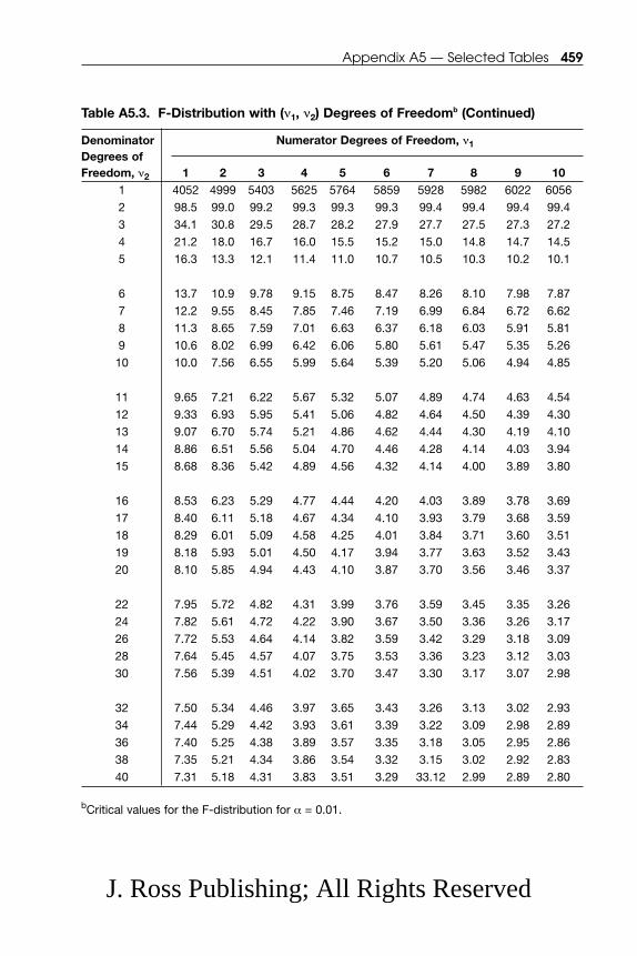
Appendix A5 — Selected Tables 459
Table A5.3. F-Distribution with (ν1, ν2) Degrees of Freedomb (Continued)
DenominatorDegrees ofFreedom, ν2 1 2 3 4 5 6 7 8 9 10
1 4052 4999 5403 5625 5764 5859 5928 5982 6022 6056
2 98.5 99.0 99.2 99.3 99.3 99.3 99.4 99.4 99.4 99.4
3 34.1 30.8 29.5 28.7 28.2 27.9 27.7 27.5 27.3 27.2
4 21.2 18.0 16.7 16.0 15.5 15.2 15.0 14.8 14.7 14.5
5 16.3 13.3 12.1 11.4 11.0 10.7 10.5 10.3 10.2 10.1
6 13.7 10.9 9.78 9.15 8.75 8.47 8.26 8.10 7.98 7.87
7 12.2 9.55 8.45 7.85 7.46 7.19 6.99 6.84 6.72 6.62
8 11.3 8.65 7.59 7.01 6.63 6.37 6.18 6.03 5.91 5.81
9 10.6 8.02 6.99 6.42 6.06 5.80 5.61 5.47 5.35 5.26
10 10.0 7.56 6.55 5.99 5.64 5.39 5.20 5.06 4.94 4.85
11 9.65 7.21 6.22 5.67 5.32 5.07 4.89 4.74 4.63 4.54
12 9.33 6.93 5.95 5.41 5.06 4.82 4.64 4.50 4.39 4.30
13 9.07 6.70 5.74 5.21 4.86 4.62 4.44 4.30 4.19 4.10
14 8.86 6.51 5.56 5.04 4.70 4.46 4.28 4.14 4.03 3.94
15 8.68 8.36 5.42 4.89 4.56 4.32 4.14 4.00 3.89 3.80
16 8.53 6.23 5.29 4.77 4.44 4.20 4.03 3.89 3.78 3.69
17 8.40 6.11 5.18 4.67 4.34 4.10 3.93 3.79 3.68 3.59
18 8.29 6.01 5.09 4.58 4.25 4.01 3.84 3.71 3.60 3.51
19 8.18 5.93 5.01 4.50 4.17 3.94 3.77 3.63 3.52 3.43
20 8.10 5.85 4.94 4.43 4.10 3.87 3.70 3.56 3.46 3.37
22 7.95 5.72 4.82 4.31 3.99 3.76 3.59 3.45 3.35 3.26
24 7.82 5.61 4.72 4.22 3.90 3.67 3.50 3.36 3.26 3.17
26 7.72 5.53 4.64 4.14 3.82 3.59 3.42 3.29 3.18 3.09
28 7.64 5.45 4.57 4.07 3.75 3.53 3.36 3.23 3.12 3.03
30 7.56 5.39 4.51 4.02 3.70 3.47 3.30 3.17 3.07 2.98
32 7.50 5.34 4.46 3.97 3.65 3.43 3.26 3.13 3.02 2.93
34 7.44 5.29 4.42 3.93 3.61 3.39 3.22 3.09 2.98 2.89
36 7.40 5.25 4.38 3.89 3.57 3.35 3.18 3.05 2.95 2.86
38 7.35 5.21 4.34 3.86 3.54 3.32 3.15 3.02 2.92 2.83
40 7.31 5.18 4.31 3.83 3.51 3.29 33.12 2.99 2.89 2.80
bCritical values for the F-distribution for α = 0.01.
Numerator Degrees of Freedom, ν1
J. Ross Publishing; All Rights Reserved

J. Ross Publishing; All Rights Reserved

2k factorial design, 344–3475M’s, 1005P’s, 10080/20 rule, 115, 118, 225
AAbsolute class frequency, 133Absolute frequency distribution, 133Abstract data, 85Accuracy, 125–126, 128Adaptation, 418Allowable spread/actual spread,
204–205Alpha risk, 233. See also Producer’s
risk; Type I errorAlternate hypothesis (H1), 233American National Standards
Institute (ANSI), 90standard symbols, 90–91
Analysis of variance (ANOVA),264–279, 327–328
F distribution, 270–271mathematical model, 271–272one-way, 266–270, 277steps, 272–273steps, using MINITAB®,
273–280table, 270, 271
Analyze phase, 15, 298–300ANOVA, 264–280
hypothesis testing, chi squaretechnique, 243–264
hypothesis testing, classictechniques, 227–243
introduction to, 211–217regression and correlation,
280–298stratification, 217–226tool selection, 213, 214, 215
Anderson-Darling normality test,274, 275
ANOVA. See Analysis of varianceANSI. See American National
Standards InstituteArithmetic mean, 145–146Assignable causes, 144Association knowledge, 281Attributes of tables, 133, 134Automobile Industry Severity
Ranking Criteria, 108Average, 145–146
BBalanced design, 333Bar graph, 139–141Basic error-proofing concept, 378Bell-shaped distribution, 137Bell Telephone Laboratories, 381Benchmarking, 354“Best in class” business, 11
461
INDEX
J. Ross Publishing; All Rights Reserved
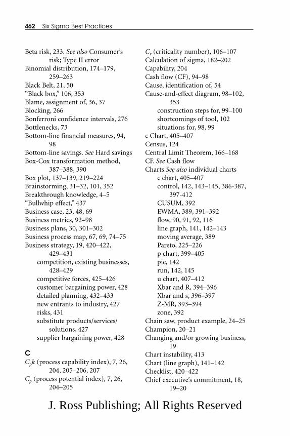
Beta risk, 233. See also Consumer’srisk; Type II error
Binomial distribution, 174–179,259–263
Black Belt, 21, 50“Black box,” 106, 353Blame, assignment of, 36, 37Blocking, 266Bonferroni confidence intervals, 276Bottlenecks, 73Bottom-line financial measures, 94,
98Bottom-line savings. See Hard savingsBox-Cox transformation method,
387–388, 390Box plot, 137–139, 219–224Brainstorming, 31–32, 101, 352Breakthrough knowledge, 4–5“Bullwhip effect,” 437Business case, 23, 48, 69Business metrics, 92–98Business plans, 30, 301–302Business process map, 67, 69, 74–75Business strategy, 19, 420–422,
429–431competition, existing businesses,
428–429competitive forces, 425–426customer bargaining power, 428detailed planning, 432–433new entrants to industry, 427risks, 431substitute products/services/
solutions, 427supplier bargaining power, 428
CCpk (process capability index), 7, 26,
204, 205–206, 207Cp (process potential index), 7, 26,
204–205
Cr (criticality number), 106–107Calculation of sigma, 182–202Capability, 204Cash flow (CF), 94–98Cause, identification of, 54Cause-and-effect diagram, 98–102,
353construction steps for, 99–100shortcomings of tool, 102situations for, 98, 99
c Chart, 405–407Census, 124Central Limit Theorem, 166–168CF. See Cash flowCharts See also individual charts
c chart, 405–407control, 142, 143–145, 386-387,
397-412CUSUM, 392EWMA, 389, 391–392flow, 90, 91, 92, 116line graph, 141, 142–143moving average, 389Pareto, 225–226p chart, 399–405pie, 142run, 142, 145u chart, 407–412Xbar and R, 394–396Xbar and s, 396–397Z-MR, 393–394zone, 392
Chain saw, product example, 24–25Champion, 20–21Changing and/or growing business,
19Chart instability, 413Chart (line graph), 141–142Checklist, 420–422Chief executive’s commitment, 18,
19–20
462 Six Sigma Best Practices
J. Ross Publishing; All Rights Reserved

Chi-square distribution table, 457Chi-square technique. See Hypothesis
testing, chi-square techniqueClass determination, 133Classic techniques. See Hypothesis
testing, classic techniquesClosed-loop data measurement
system, 86–88Coefficient of correlation (r), 293,
296–298Coefficient of correlation, square
root, coefficient ofdetermination (√r2 = r), 282
Coefficient of determination(adjusted) [(r2(Adj)], 282,295
Coefficient of determination (r2),282, 294–297
Common cause, 81Competitive forces, 425–429Completely randomized single-factor
experiment, 324–325Components of variance, 326Conditional mean, 288Conditional probability distribution,
288Confidence interval, 127Conflicting objectives, 73Constraint monitoring, 370–375Consumer’s risk, 231, 233. See also
Beta risk; Type II errorContact flow chart, 116Continuous data control charts,
386–397Continuous improvement
process, 97–98program, 63
Continuous probability distribution,258–259
Continuous process database metrics,192–199
Continuous quantitative groupingtype, 133
Continuous variable, 83, 159Control chart, 142, 143–145
continuous data, 386–397development methodology/
classification, 384–386discrete data, 397–412hypothesis testing, 386
Control chart hypothesis testing, 386Control chart tool, 384–386Control phase, 15–16, 420–422
checklist, 420–422error proofing, 375–380, 375–380final project summary, 414–419introduction to, 367–368monitor constraints, 370–375self-control, 368–370statistical control process
techniques, 380–413Control plan, 360Core team members, 44Correlation analysis, 293–298Correlation and regression, 280–298Cost/benefit analysis, 358–359,
360–362Cost reduction, 415Creative thinking, 352Criticality number (Cr), 106–107“Critical path,” 46Critical to quality (CTQ)
characteristics, 56–57, 353customers and, 56–57, 64–65, 66,
74defining, three-step process,
57–66definition of, 53, 68identification of customer, 57–58research customer, 59–64translate customer information,
64–66
Index 463
J. Ross Publishing; All Rights Reserved

Critical to quality concept, 9CSR. See Customer service
representative CTQs. See Critical to quality
characteristicsCumulative density function,
172–174Cumulative sum (CUSUM) chart,
392Current Sigma metrics, 200–202Customer, 54–66
CTQs and, 56–58data, 59–62, 64–65needs, 7, 8research, 59, 60, 62–63satisfaction, 63, 64types, 55–56
Customer service representative(CSR), 308–309
Customization, 418CUSUM chart. See Cumulative sum
chartCycle time, 72
DD. See Detection ability Data
collection plan, 121–131on customer, 59–62dimension and qualification,
85–86plotting of, 284presentation plan, 131–148questions answered, 30–31raw vs. summarized, 241types, 83–85
Defect rate. See Defects per millionopportunities (DPMO);Errors per millionopportunities (EPMO)
Defects, 3–4, 8–9, 24–25, 72–73, 302
Defects per million opportunities(DPMO), 182–189
Defining customer CTQs, 57–66identify customer, 57–58research customer, 59–64translate customer information,
64–66Define-Measure-Analyze-Design-
Verify (DMADV), 13–14Define-Measure-Analyze-Improve-
Control (DMAIC), 14–16,67, 355. See also individualphases of DMAIC
Define phase, 14–15, 74customer, the, 54–66detailed process mapping, 69–74high-level process, 67–69introduction to, 53–54
Degrees of correlation, 294Degrees of freedom (df), 270, 271Delay time, 72“Deliverables,” 46Deming, W. Edwards, 381Dependency, 319–320Dependent variable, 78, 282, 333Deployment flow chart, 90Design for Six Sigma (DFSS), 9,
13–14Design of experiments (DOE), 303,
323–347completely randomized single-
factor experiment, 324–325dependency and, 320factorial experiments, 330–332introduction to, 323–324quantitative relationship and, 227random effect model, 325–330terminology for, 332–334three-factor factorial
experiments, 340–344
464 Six Sigma Best Practices
J. Ross Publishing; All Rights Reserved

two-factor factorial experiments,334–340
2k factorial design, 344–347Design specification, 6, 7Design tolerance, 7Detailed process flow chart, 90Detection ability (D), 109Deterministic relationship, 282df. See Degrees of freedom DFSS. See Design for Six Sigma Dichotomous qualitative variable, 82Differentiation, 429, 430Direct replication, 418Discrete data control charts, 397–412Discrete distribution, 258–259Discrete process sigma conversion
table, 184–185Discrete variable, 83DMADV. See Define-Measure-
Analyze-Design-Verify DMAIC. See Define-Measure-
Analyze-Improve-Control Documentation, 414–416DOE. See Design of experiments DPMO. See Defects per million
opportunities
EEdge-peaked distribution, 137Effectiveness of measures, 82Efficiency of measures, 8280/20 rule, 115, 118, 225Employee
errors, 376–377“ownership,” 369, 370process breakdown/structure, 360role, 19, 310self-control for process, 368–370
EMS. See Error mean squareEPMO. See Errors per million
opportunities
Epsilon-square (ε2) statistic, 273Error mean square (EMS), 269. See
also Unexplained variationError proofing, 375–380Error-proofing tools, 378–380Error sum of squares (ESS), 269, 341Errors and mistakes, 9Errors per million opportunities
(EPMO), 189–191ESS. See Error sum of squaresEstimation bias, 124Evolution of improvement strategy,
305EWMA. See Exponentially weighted
moving average chartExclusion bias, 125Executive leadership, 18, 19–20Expected benefits, 43–44, 415Experiment, 323Experimental error, 269Experimental run (test run), 333Expert, 21, 23Explained variation, 267, 294–295Exponential distribution, 171–174Exponentially weighted moving
average (EWMA) chart, 389,391–392
External customer, 55Extreme values, 145, 146
FFactor, 333Factorial effect, 344Factorial experiment, 330–344
main effect, 330–331model adequacy checking, 337three-factor experiment, 340–344two-factor experiment, 334–3372k factorial design, 344–348, 349
Factorial k1 � k2 � k3 ..., 333Failure definition, 115, 116
Index 465
J. Ross Publishing; All Rights Reserved

Failure Mode and Effects Analysis(FMEA)
example, 112–113, 114iterative process, 353modified, 113, 115–121steps in, 109, 112
Failure Mode, Effects, and CriticalityAnalysis (FMECA), 103–109
criticality assessment, 106–109,110–111
design information, 106guidance, 105–106historical information, 104key functions, 104methodology, 105users of, 104
Fair dice, 159False conclusion, 412–413F-distribution, 270–271, 458-459Feedback loop, 369–370, 372–373Financial benefits, 45, 359, 415. See
also ProfitabilityFishbone diagram. See Cause-and-
effect diagram5Ms, 1005Ps, 100Fixed-effect model, 325Flow chart. See also Process mapping
for analysis, 215ANSI, standard symbols for,
90–91contact flow chart, 116definition of, 89detailed process flow chart, 90finished product, symbols, 92for improvement strategy, 305process flow chart, 91, 92top-down flow chart, 90types, process analysis, 90
Flow diagramming, 70
FMEA. See Failure Mode and EffectsAnalysis
FMECA. See Failure Mode, Effects,and Criticality Analysis
Focus, 429, 431Future projects, 419
GGamma distribution, 159, 175–177,
208Gap analysis, 64, 116, 118Gaussian distribution. See Normal
distributionGE, 3, 17Generic strategic approach, 429Global logistics, 436–437Goal Sigma metrics, 200–202Goal statement, 48Goodness-of-fit test, 258–264Green Belt, 21, 49Grouped bar graph, 141Growing and/or changing business,
19
HH0 (null hypothesis), 233, 258H1 (alternate hypothesis), 233Hammer, Michael, 12Hard savings, 26, 29High-level process map, 67–69. See
also Process mappingHistogram, 135–137, 219–224History of Six Sigma, 2–3Hypothesis testing, chi-square
technique, 249–263goodness-of-fit test, 258–263making inferences, greater than
two population proportions,249–251
making inferences, populationvariance, 251–258
466 Six Sigma Best Practices
J. Ross Publishing; All Rights Reserved

testing independence, twoqualitative populationvariables, 244–249
Hypothesis testing, classic techniques,227–243
hypothesis testing, populationmean, 235–241
hypothesis testing, proportionmean, 241–243
mathematical relationshipsamong summary measures,228–230
theory, 230–235
II. See InventoryIdentify customer, CTQ, 57–58Implementation structure, Six Sigma,
16–22prerequisites for, 17roles and responsibilities, 18–22
Implemented process instructions, 416–417training, 417
Implementing alternative solution,359–360
Improvement, 200Improvement process stages, 348, 350Improvement strategies
determining, cases, 321–323evolution of, 305factors and alternatives, 319–323list, 303
Improve phase, 15, 363–365conceptual summary, 362–363DOE, introduction to, 323–348improvement strategies,
factors/alternatives, 319–323introduction to, 301–305overview of topics, 351–363process reengineering, 305–319
solution alternatives, 348–351Inclusion bias, 125Independent observer, 129Independent variable, 78, 282,
332–333Infant business, 19Input measures, 78Input-Process-Output (IPO) process,
27–28, 30, 35, 439, 441–442Inputs and outputs, 4, 8, 79, 80Internal customer, 55Inter quartile range (IQR), 139Interval data, 84Inventory (I), 94–98IPO. See Input-Process-Output
processIQR. See Inter quartile rangeIshikawa, Dr. Kaoru, 98Isolated peak distribution, 137
JJIT. See Just-In-Time trainingJuran, Joseph M., 381Just-In-Time (JIT) training, 21
KKano’s theory, 63Key guiding elements, 16Kodak, 3
LLack of accuracy, 126Lack of precision, 126Lambda value, 387–389Large-population case, 164, 228, 229Least squares method, 284–286, 287,
290Level, 333Line graph (chart), 141, 142–143Logistics network, 436Long-term Sigma values, 198Losses, 25. See also Defects
Index 467
J. Ross Publishing; All Rights Reserved

Lower specification limit (LSL), 6Lower-tail hypothesis test, 254–255LSL. See Lower specification limit
MMaintenance training, 417–418Malcolm Baldrige National Quality
Award, 2Manageable problem, 36, 37Management philosophy, 10Manufacturing cycle time, 72Manufacturing strategy, 435–436Margin of error, 155, 157Master, 21, 23Master Black Belt, 21, 50Matured business, 19Mean, 5, 145–146Mean square, 270Measurable problem, 36, 37Measure, 204–205Measure phase, 15, 208–209
data collection plan, 121–131data presentation plan, 131–148foundation of, 79–88introduction to, 77–79measuring tools, 89–121MINITAB®, introduction to,
148–155probabilistic data distribution,
158–181process capability/process
performance indices,202–208
sample size determination,155–158
sigma, calculation of, 182–202Measuring tools
business metrics, 92–98cause-and-effect diagram, 98–102flow charting, 89–92, 93FMEA, 103, 109–121
FMECA, 103–109Median, 146Method of least squares, 284–286,
287, 290Microsoft®, Excel, 192Microsoft®, Office, 379Military/Government Severity
Ranking Criteria, 109MIL-STD-1629A/Notice 2, 104, 106MINITAB® software, 148–155Missing data bias, 126Mission statement, 27, 35–40Mistakes and errors, 9Mode, 146–146Modified FMEA, 113, 115_120Monitoring constraints, 370–375Motorola, 2–3, 6–8, 11–12, 17,
199–200Motorola’s quality level commitment,
2–3Moving average chart, 389Multimodal frequency distribution,
137, 220Multiqualitative variables, 82
NNational Quality Month, 2Negative estimate of variance
component, 328Negative perfect correlation, 294Net profit (NP), 94–98NGT. See Nominal group techniqueNominal data, 83Nominal group technique (NGT),
32–34, 35Nonsense correlation, 297Nontechnical processes, 8Nonuniformity, 5Non-value-added activities, 13,
307–308, 309Normal distribution, 5, 6, 159–168
468 Six Sigma Best Practices
J. Ross Publishing; All Rights Reserved

Normally distributed population, 263NP. See Net profitNull hypothesis (H0), 233, 258
OObservable problem, 36, 37OC function. See Operating
characteristic (OC function)OE. See Operating expenseOne-factor ANOVA. See One-way
ANOVAOne-sided hypothesis, 235One-tail test, 235One-way ANOVA, 266–270, 277, 325OOC conditions. See Out-of-control
conditionsOperating characteristic (OC
function), 233Operating expense (OE), 94–98Operational level, 442Operational measures, change in, 94,
98Opportunity statement, 48, 49Order to cash (revenue) cycle, 72Ordinal data, 84Out-of-control (OOC) conditions,
144, 384Output measures, 78Overall cost leadership, 429–430
PPareto, Vilfredo, 115Pareto chart, 225–226Parts per million (PPM), 6, 197, 199,
206Pay-off matrix, 359, 360p Chart, 399–405
with variable sample size,403–405
Pearson’s Sample Coefficient ofCorrelation, 296
Pie chart, 142
Pilot-testing alternatives, 356–358Pilot test/simulation, 157Plateau distribution, 137Poisson distribution, 168–171Pooled standard deviation, 329, 330Poor business performance signs, 10,
11Population variance, 251–252, 254Population mean hypothesis testing,
235–237Population proportions, 243, 249, 298Population regression line, 288Population standard error of the
estimate, 288Positive perfect correlation, 294Power, 233Power chain saw product example,
24–25Power of the test, 232Pp (process performance), 206–207Ppk (process performance index),
206–207PPM. See Parts per millionPrecision, 125–126Predicted variable, 282Prediction interval, 289–290Predictor variable, 282Presentation of data, 131–147Preventive maintenance training, 417Prioritized data, 353Probabilistic data distribution,
158–181binomial distribution, 174–179exponential distribution,
171–174normal distribution, 159–168Poisson distribution, 168–171Weibull distribution, 179–181
Probability density function, 180Problem-solving process, 354–355Problem statement, 35–40, 99
Index 469
J. Ross Publishing; All Rights Reserved

Process, 80, 81, 413Process activities, 12–13, 307–309Process analysis, 309–310Process capability, 9, 205Process capability index (Cpk), 7, 26,
204, 205–206, 207Process capability (Cp and Cpk) index,
204Process centering, 305–307Process flow chart, 91, 92Process improvement, 155Process mapping, 69–74, 351–352. See
also High-level process mapterminology, 72–73uses of, 89
Process mean, 393Process measures, 78Process monitoring, 374–376Process performance index (Ppk),
206–207Process performance (Pp), 206–207Process potential index (Cp), 7, 26,
204–205Process/product cost analysis, 354Process reengineering, 12, 305–319
analysis of process, 309–310process activities, 307–309process centering, 305–307steps, high-level listing, 310–312warehouse exercise, 312–319
Process resource analysis, 306–307Process Sigma (ST) value, 185, 187,
191, 201–202Process standard deviation, 393, 394Process time, 72Process variation limits, 7Producer’s risk, 230, 233Product design specification, 7Production system, 439–442Productivity, 98Product life cycle, 106, 107, 179–180
Product reviews/audits, 30Product risk, 103Product/service delivery cycle,
439–442Product specification, 7Professional bias, 126Professional employee, 309–310Profitability, 14. See also Financial
benefitsProfit margin, 9Project
activities, 47charter, 48, 49closure, checklist, 419criteria, 22–25documentation, 414–416final summary, 414–419, 420implementaton, 359–360leader, 46planning and management,
42–47plan/time line, 48proposal, 42–45selection, 23, 38
Proportion defective data, 399–400Proportion mean hypothesis testing,
241–243
QQuadratic regression equation,
296–297Qualitative analysis tools, 298–299Qualitative grouping type, 133Qualitative measure, 82Qualitative population variables, 243,
244–245, 298Quality
control, 370costs and losses, 25issues impacting, 25key components of, 3
470 Six Sigma Best Practices
J. Ross Publishing; All Rights Reserved

Quality improvement process, 12Quantitative grouping type, 133Quantitative measure, 82–83Quartile values, 137–139
Rr (coefficient of correlation), 293,
296–298r2(Adj) (coefficient of determination,
adjusted), 282, 295r2 (coefficient of determination), 282,
294–297Random effect model, 325–330Randomization, 266Randomness, 126Range, 147Ratio data, 84–85RCFA. See Root cause failure analysis“Reasonable results,” 166Reengineering, 12. See also Process
reengineeringReference standard, 81Regression, 280–282Regression analysis, 281Regression and correlation, 280–298Regression equation, 282, 286,
297–298, 299Regression line, 282, 284–285, 286,
288–289Regular service maintenance training,
418Relative frequency distribution, 133Remedy, suggestion of, 36, 37, 39Repeatability, 127Repetition, 333Replication, 333, 418Replication opportunities, 414, 418,
420Representative of population,
126–127Reproducibility, 127–128
Research customer, CTQ, 59-64Residuals, 278, 337, 338–339Residual variation, 269Resource assessment, 359Resource monitoring, 371–375Resource utilization, 370Return on assets (ROA), 94–98Return-on-investment (ROI), 19Revenue increase, 415Revenue (order to cash) cycle, 72Risk analysis, 355–356Risk priority number (RPN),
107–109, 110–111Risks, 351, 431ROA. See Return on assetsROI. See Return on investmentRoot cause failure analysis (RCFA),
115, 118Root cause of problem, 22, 41, 98,
144, 353RPN. See Risk priority numberRun chart, 142, 145
SSample mean, 126, 158Sample size determination, 155–158Sampling, 124Sampling error, 269Scatter diagram, 284Schematic box plot, 138–139Scope, 48Self-control, 368–370SE mean. See Standard error of the
meanService maintenance training, 418Severity (S), 109Shewhart, Walter A., 381Shewhart Control Charts, 413Short-term Sigma values, 198Sigma, 5–6
Index 471
J. Ross Publishing; All Rights Reserved
Sigma metrics value calculation,182–202
DPMO, 182–189EPMO, 189–191Motorola’s 1.5 sigma shift
concept, 199–200Sigma shift, 199–202Significance level, 232Significant difference, 233Simple correlation analysis, 282,
293–298Simple regression analysis, 282–293Simulation, 320Simulation tool, 356SIPOC. See Supplier-Input-Process-
Output-CustomerSix Sigma
behavioral change issues, 12bottom line of, 350–351elements to avoid, 16high level, 9history, 2–3implementation structure, 16–22key concepts, 8–9, 11–13management philosophy, 10–11metric, 9at Motorola, 2–3, 6–8, 11–12, 17,
199–200process road map, 13–16project charter, 48, 49project criteria, 22–40project planning/management,
42–47series yield concept, 187–189statistical, 6–7, 9, 23–24strategy, 9team selection, 40–41
Skewed distribution, 137Slope, 283–284Small-population case, 228, 229Society of Automotive Engineers, 103
Soft savings, 26, 29Software. See MINITAB® softwareSolution alternatives, 348–351SPC. See Statistical process control
techniquesSpecial cause, 81Specific problem, 35, 37Spurious correlation, 297SS. See Sum of squaresStability, 128Stable operation, 9Stacked bar graph, 139–141Stakeholder, 56Standard deviation, 147–148. See also
SigmaStandard error, 155Standard error of the mean (SE
mean), 155States of business, 19Statistically designed experiment, 102Statistical process control (SPC)
techniquescontinuous data control chart,
386–397control chart development,
384–386discrete data control charts,
397–412general chart analysis, 412–414impact on controlling process
performance, 382–384introduction to, 380–381process variation causes, 381–382
Statistical software applications. SeeMINITAB® software
Steering committee, 18, 20Stochastic relationship, 282Strategic level, 442Strategy. See Business strategyStratification, 135, 217–226
advantages of, 218–219
472 Six Sigma Best Practices
J. Ross Publishing; All Rights Reserved

elements commonly used, 219Pareto chart and, 225–226process shortcomings, 222process steps, 218
Summary measures, 228–230Sum of squares (SS), 270, 271, 341Supplier-Input-Process-Output-
Customer (SIPOC)measurement, stages in, 78tractor dealer example, 69, 70
Supply chain, 436Support services, 439–442
TT. See Throughput Tables, 133–135, 456-459
t-distribution table, 456Tactical level, 442Team
leader, 21members, 22, 23, 48selection, 40–41
Technical process, 8Test of independence, 263Test run (experimental run), 333Test statistic, 233Three-factor factorial experiments,
340–344Throughput (T), 94–98TMS. See Treatments mean squareTOFD. See Total opportunities for
defectsTOFE. See Total opportunities for
errorsTop-down flow chart, 90Total opportunities for defects
(TOFD), 182–183Total opportunities for errors
(TOFE), 189Total SS. See Total sum of squaresTotal sum of squares (Total SS), 270
Trade-off concept, 231Translate customer information,
CTQ, 64–66Treatment combination, 333, 344Treatments mean square (TMS), 269Treatments sum of squares (TSS), 268Treatment variation, 267Trends, 412Trimean, 154–155True mean, 126True regression line, 286, 288–289,
290–293Truncated distribution, 137TSS. See Treatments sum of squares t-Test, 238, 240–241Twentieth century productivity
efforts, 3–4Two-factor ANOVA. See Two-way
ANOVATwo-factor factorial experiment,
334–3402k factorial design, 344–347Two-sided hypothesis, 234Two-tail hypothesis test, 254, 257–258Two-way ANOVA, 321, 334–337Type I error, 230, 233Type II error, 231, 233Typical product life cycle, 106, 107
Uu Chart, 407–412
with variable sample size,411–412
Unbalanced design, 333Unbiased sampling data, 124–125,
131Underlying population distribution,
259Unexplained variation, 269, 294. See
also Error mean square
Index 473
J. Ross Publishing; All Rights Reserved

Uniformly distributed population,263
Unimodal distribution, 220Upper specification limit (USL), 6Upper-tail hypothesis test, 254,
255–256U.S., business efforts during twenty-
first century, 436USL. See Upper specification limitU.S. Military Standard 1629, 104
VValue-added activities, 12, 13,
307–308Variability, 5Variable data, 8Variance, 147Variance components, 327–328Variation, 9, 381–382
WWarehouse exercise, 312–319Waste, 13, 307Weak correlation, 294Weibull distribution, 179–181Workers. See Employee
XXbar and R charts, 394–396Xbar and s chart, 396–397Xerox, 3, 17
ZZero correlation, 294Zero defects, 6, 9, 12, 200Z-MR chart, 393–394Zone chart, 392Z-test, 237–238
474 Six Sigma Best Practices
J. Ross Publishing; All Rights Reserved

J. Ross Publishing; All Rights Reserved

J. Ross Publishing; All Rights Reserved

J. Ross Publishing; All Rights Reserved

J. Ross Publishing; All Rights Reserved