NBER WORKING PAPER SERIES

SIZE AND VALUE IN CHINA

Jianan LiuRobert F. Stambaugh

Yu Yuan

Working Paper 24458http://www.nber.org/papers/w24458

NATIONAL BUREAU OF ECONOMIC RESEARCH1050 Massachusetts Avenue

Cambridge, MA 02138March 2018, Revised December 2018

We are grateful for comments from the referee (Eugene Fama), Jules van Binsbergen, Danting Chang, Zhi Da, Zhe Geng, Dong Lou, Amir Yaron, Jianfeng Yu, seminar participants at the Wharton School, and conference participants at the 2018 Johns Hopkins Carey Finance Conference. Yuan gratefully acknowledges financial support from the NSF of China (71522012). The views expressed herein are those of the authors and do not necessarily reflect the views of the National Bureau of Economic Research.

NBER working papers are circulated for discussion and comment purposes. They have not been peer-reviewed or been subject to the review by the NBER Board of Directors that accompanies official NBER publications.

© 2018 by Jianan Liu, Robert F. Stambaugh, and Yu Yuan. All rights reserved. Short sections of text, not to exceed two paragraphs, may be quoted without explicit permission provided that full credit, including © notice, is given to the source.

Size and Value in ChinaJianan Liu, Robert F. Stambaugh, and Yu Yuan NBER Working Paper No. 24458March 2018, Revised December 2018JEL No. G12,G15,G18

ABSTRACT

We construct size and value factors in China. The size factor excludes the smallest 30% of firms, which are companies valued significantly as potential shells in reverse mergers that circumvent tight IPO constraints. The value factor is based on the earnings-price ratio, which subsumes the book-to-market ratio in capturing all Chinese value effects. Our three-factor model strongly dominates a model formed by just replicating the Fama and French (1993) procedure in China. Unlike that model, which leaves a 17% annual alpha on the earnings- price factor, our model explains most reported Chinese anomalies, including profitability and volatility anomalies.

Jianan LiuFinance Department, The Wharton School University of Pennsylvania Philadelphia, PA 19104-6367jiananl@wharton.upenn.edu

Robert F. StambaughFinance DepartmentThe Wharton SchoolUniversity of Pennsylvania Philadelphia, PA 19104-6367and NBERstambaugh@wharton.upenn.edu

Yu YuanShanghai Advanced Institute of FinanceShanghai Jiao Tong UniversityDatong Plaza, 211 West Huaihai Road, ShanghaiP.R.China, 200030yyuan@saif.sjtu.edu.cn

1. Introduction

China has the world’s second-largest stock market, helping to finance an economy that

some predict will be the world’s largest within a decade.1 China also has political and

economic environments quite different from those in the US and other developed economies.

Moreover, China’s market and investors are separated from the rest of the world. China

largely prohibits participation by foreign investors in its domestic stock market as well as

participation by its domestic investors in foreign markets.2

Factor models provide a cornerstone for investigating financial asset pricing and for de-

veloping investment strategies. Many studies of China’s stock market use a three-factor

model constructed by following the Fama and French (1993) procedure for US factors.3

The advisability of simply replicating a US model in China is questionable, however, given

China’s separation and the many differences in economic and financial systems. We explore

and develop factor models in China, allowing its unique environment to dictate alternative

approaches.

We start by examining size and value effects in the Chinese market. These two effects have

long been recognized elsewhere as important characteristics associated with expected return:

Banz (1981) reports a firm-size effect, and Basu (1983) finds an effect for the earnings-price

ratio, a popular value metric. Size and value are the most prominent characteristics used

by many institutions to classify investment styles. The most widely used nonmarket factors

in academic research are also size and value, following the influential study by Fama and

French (1993). Our study reveals that size and value effects are important in China but with

properties different from the US. We construct size and value factors for China.

The size factor is intended to capture size-related differences in stock risk and return

that arise from size-related differences in the underlying businesses. In China, however,

the stock of a small listed firm is typically priced to reflect a substantial component of value

related not to the firm’s underlying business but instead to the Chinese initial public offering

1According to the World Bank, the 2016 equity values of listed domestic companies, in trillions of US dol-lars, are 27.4 in the US and 7.3 in China, followed by 5.0 in Japan. For a forecast that China’s gross domesticproduct will reach that of the US by 2028, see Bloomberg ( https://www.bloomberg.com/graphics/2016-us-vs-china-economy/).

2At the end of 2016, 197 foreign institutions were authorized to invest in A-shares, China’s domesticallytraded stocks, but with a quota of just 0.6% of total market value (and even less in earlier years). Chinesedomestic investors can invest in international financial markets only through a limited authorized channel.

3Examples of such studies include include Yang and Chen (2003), Fan and Shan (2004), Wang and Chin(2004), Chen et al. (2010), Cheung, Hoguet, and Ng (2015), and Hu et al. (2018).

1

(IPO) process. In China, the IPO market is strictly regulated, and a growing demand for

public listing confronts the low processing capacity of the regulatory bureau to approve IPOs.

As a consequence, private firms seek an alternative approach, a reverse merger, to become

public in a timely manner. In a reverse merger, a private firm targets a publicly traded

company, a so-called shell, and gains control rights by acquiring its shares. The shell then

buys the private firm’s assets in exchange for newly issued shares. While reverse mergers

occur elsewhere, IPO constraints are sufficiently tight in China such that the smallest firms

on the major exchanges become attractive shell targets, unlike in the US, for example.

The smallest listed firms are the most likely shells. In fact, 83% of the reverse mergers

in China involve shells coming from the smallest 30% of stocks. For a typical stock in the

bottom 30%, we estimate that roughly 30% of its market value reflects its potential shell

value in a reverse merger. Our estimate combines the empirical probability of being targeted

in a reverse merger with the average return accompanying that event. Consistent with the

contamination of small-firm stock prices by shell value, we also find that when compared to

other firms, the smallest 30% have returns less related to operating fundamentals, proxied

by earnings surprises, but more related to IPO activity. Therefore, to avoid shell-value

contamination when constructing any of our factors, we delete the bottom 30% of stocks,

which account for 7% of the stock market’s total capitalization.

The value effect in China is best captured by the earnings-price (EP ) ratio, versus other

valuation ratios. Following Fama and French (1992), we treat the choice among alternative

valuation ratios as an empirical question, asking which variable best captures the cross-

sectional variation in average stock returns. As in that study, we run a horse race among

all candidate valuation ratios, including EP , book-to-market (BM), asset-to-market, and

cash-flow-to-price ratios. In a Fama-MacBeth regression including those four ratios, EP

dominates all others, just as Fama and French (1992) find BM dominates in the US market.

Relying on the latter US result, Fama and French (1993) use BM to construct their value

factor. Relying on our result for China, we use EP to construct our value factor.

Size and value are important factors in China, as revealed by their average premiums as

well as their contributions to return variance. Our size and value factors both have average

premiums exceeding 1% per month over our 2000–2016 sample period. For the typical

stock in China, size and value jointly explain an additional 15% of monthly return variance

beyond what the market factor explains. In comparison, size and value explain less than

10% of additional return variance for the typical US stock during the same period.

Our three-factor model, CH-3, includes the market factor as well as size and value factors

2

incorporating the above China-specific elements. For comparison, we construct an alternative

three-factor model, FF-3, by simply replicating the Fama and French (1993) procedure. We

find that CH-3 strongly dominates FF-3. Specifically, FF-3 cannot price the CH-3 size and

value factors, which have (significant) FF-3 annualized alphas of 5.6% and 16.7%. In contrast,

CH-3 prices the FF-3 size and value factors, which have (insignificant) CH-3 annualized

alphas of just −0.5% and 4.1%. A Gibbons, Ross, and Shanken (1989) test of one model’s

ability to price the other’s factors gives a p-value of 0.41 for CH-3’s pricing ability but less

than 10−12 for FF-3’s ability.

We also investigate the ability of CH-3 to explain previously reported return anomalies

in China. A survey of the literature reveals anomalies in nine categories: size, value, prof-

itability, volatility, return reversal, turnover, investment, accruals, and illiquidity. We find

each of the first six categories contains one or more anomalies that produce significant long-

short alphas with respect to the single-factor capital asset pricing model (CAPM). CH-3

accommodates all anomalies in the first four of those six categories, including profitability

and volatility, whose anomalies fail FF-3 explanations in the US. CH-3 fails only with some

of the reversal and turnover anomalies. In contrast, FF-3 leaves significant anomalies in

five of the six categories. A total of ten anomalies are unexplained by the CAPM; CH-3

explains eight of them, while FF-3 explains three. The average absolute CH-3 alpha for the

ten anomalies is 5.4% annualized, compared to 10.8% for FF-3 (average absolute t-statistics:

1.12 versus 2.70).

Hou, Xue, and Zhang (2015) and Fama and French (2015) add two factors based on

investment and profitability measures in their recently proposed factor models, Q-4 and FF-

5. Investment does not produce a significant CAPM alpha in China, and profitability is fully

explained by CH-3. In an analysis reported in the Appendix, we find that a replication of

FF-5 in China is dominated by CH-3.

Overall, CH-3 performs well as a factor model in China, and it captures most documented

anomalies. In US studies, researchers often supplement the usual three factors (market, size,

and value) with a fourth factor, such as the momentum factor of Carhart (1997) or the

liquidity factor of Pastor and Stambaugh (2003). We also add a fourth factor, motivated

by a phenomenon rather unique to China: a stock market dominated by individuals rather

than institutions. Over 101 million individuals have stock trading accounts in China, and

individuals own 88% of the market’s free-floating shares. This heavy presence of individuals

makes Chinese stocks especially susceptible to investor sentiment. To capture sentiment

effects, we base our fourth factor on turnover, which previous research identifies as a gauge

3

of both market-wide and stock-specific investor sentiment (e.g., Baker and Stein, 2004; Baker

and Wurgler, 2006; Lee, 2013). The resulting four-factor model, CH-4, explains the turnover

and reversal anomalies in addition to the anomalies explained by CH-3, thereby handling all

of China’s reported anomalies.

The remainder of the paper proceeds as follows. Section 2 discusses data sources and

sample construction. Section 3 addresses the interplay between firm size and China’s IPO

constraints and explores the importance of shell-value distortions in small-stock returns.

Section 4 investigates value effects in China. In Section 5, we construct CH-3 and FF-3

and compare their abilities to price each other’s factors. In Section 6, we compare the

abilities of those three-factor models to price anomalies. In Section 7, we construct CH-4 by

including a turnover factor and then analyze the model’s additional pricing abilities. Section

8 summarizes our conclusions.

2. Data source and samples

The data we use, which include data on returns, trading, financial statements, and

mergers and acquisitions, are from Wind Information Inc. (WIND), the largest and most

prominent financial data provider in China. WIND serves 90% of China’s financial institu-

tions and 70% of the Qualified Foreign Institutional Investors (QFII) operating in China.

The period for our main analysis is from January 1, 2000, through December 31, 2016.

China’s domestic stock market, the A-share market, began in 1990 with the establishment

of the Shanghai and Shenzhen exchanges. We focus on the post-2000 period for two reasons.

The first is to assure uniformity in accounting data. The implementation of rules and

regulations governing various aspects of financial reporting in China did not largely take

shape until about 1999. Although 1993 saw the origination of principles for fair trade and

financial disclosure, firms received little guidance in meeting them. Companies took liberties

and imposed their own standards, limiting the comparability of accounting data across firms.

Not until 1998 and 1999 were laws and regulations governing trading and financial reporting

more thoroughly designed and implemented. For example, detailed guidelines for corporate

operating revenue disclosure were issued in December 1998 and implemented in January

1999. Securities laws were passed in December 1998 and implemented in July 1999. Only by

1999 did uniformity in accounting standards become widely accomplished. Because portfolios

formed in 2000 use accounting data for 1999, our post-2000 sample for portfolio returns relies

on accounting data more comparable across firms than in earlier years.

4

The second reason for beginning our sample in 2000 is to ensure sufficient numbers of

observations. Portfolios are used in our study to construct factors and conduct many of the

tests. To enable reasonable precision and power, we require at least 50 stocks in all portfolios

after imposing our filters, which include eliminating stocks (i) in the bottom 30% of firm

size, (ii) listed less than six months, and (iii) having less than 120 trading records in the

past year or less than 15 trading records in the past month. This last pair of conditions

is intended to prevent our results from being influenced by returns that follow long trading

suspensions. Only by 1999 do the numbers of stocks in the market allow these criteria to be

met.

WIND’s data on reverse mergers begin in 2007, when the China Securities Regulatory

Commission identified the criteria of a merger and acquisition (M&A) proposal that classify

it as a reverse merger, making such deals easier to trace. In Section 3.2, we use reverse

merger data to estimate shell values. Additional details about the data and the construction

of empirical measures are provided in the Appendix.

3. Small stocks and IPO constraints

Numerous studies in finance address China’s unique characteristics. For example, Allen,

Qian, and Qian (2003, 2005) compare China to other developed countries along various po-

litical, economic, and financial dimensions. Brunnermeier, Sockin, and Xiong (2017) study

China’s government interventions in its trading environment. Bian et al. (2017) show the

special nature of leveraged investors in China’s stock market. Song and Xiong (2018) em-

phasize the necessity of accounting for the economy’s uniqueness when analyzing risks in

China’s financial system. Allen et al. (2009) and Carpenter and Whitelaw (2017) provide

broader overviews of China’s financial environment.

One aspect of the Chinese market especially relevant for our study is the challenge faced

by firms wishing to become publicly traded. As discussed earlier, market values of the

smallest firms in China include a significant component reflecting the firms’ potential to be

shells in reverse mergers. Private firms often employ reverse mergers to become publicly

traded rather than pursue the constrained IPO process. Section 3.1 describes that IPO

process, while Section 3.2 describes reverse mergers and presents a notable example of one in

China. In Section 3.3, we compute a simple estimate of the fraction of firm value associated

with being a shell for a potential reverse merger, and we find the fraction to be substantial for

the smallest stocks. Consistent with that result, we show in Section 3.4 that the returns on

5

those stocks exhibit significantly less association with their underlying firms’ fundamentals.

Our evidence demonstrating the importance of the shell component of small-firm values

is buttressed by contemporaneous research on this topic, conducted independently from ours.

In a study whose principal focus is the importance of shell values in China, Lee, Qu, and Shen

(2017) also show that the shell component is a substantial fraction of small-firm values and

that, as a result, the returns on small-firm stocks exhibit less sensitivity to fundamentals but

greater sensitivity to IPO activity. Lee, Qu, and Shen (2017) explore models for pricing the

shell-value firms, whereas we focus on models for pricing the “regular” stocks constituting

the other 93% of the stock market’s value.

3.1. The IPO process

In China, the IPO market is controlled by the China Securities Regulatory Commission

(CSRC). As a central planner, the CSRC constrains the IPO process to macro-manage the

total number of listed firms (e.g., Allen et al., 2014). Unlike the US, where an IPO can

clear regulatory scrutiny in a matter of weeks, undertaking an IPO in China is long and

tedious, easily taking three years and presenting an uncertain outcome. As detailed in the

Appendix, the process involves seven administrative steps, three bureau departments, and a

select 25-member committee that votes on each application. The committee meets for both

an initial review and a final vote, with those meetings separated by years. As of November

2017, the CSRC reported 538 firms being processed, with just 31 having cleared the initial

review. The IPOs approved in early 2017 all entered the process in 2015.

The long waiting time can impose significant costs. During the review process, firms are

discouraged from any sort of expansion and must produce consistent quarterly earnings. Any

change in operations can induce additional scrutiny and further delay. A firm undertaking

an IPO may thus forgo substantial investment opportunities during the multi-year approval

process. Moreover, policy changes can prolong the process even more. In 2013, the CSRC

halted all reviews for nearly a year to cool down the secondary market.

3.2. Reverse mergers

Facing the lengthy IPO process, private firms wishing to become public often opt for

an alternative: reverse merger. A reverse merger, which is regulated as an M&A, involves

fewer administrative steps and is much faster. We illustrate the process via a real-life case

involving the largest delivery company in China, SF Express (SF).

6

In 2016, SF decided to become public through a reverse merger. To be its shell firm,

SF targeted the small public company, DT Material (DT), with market value of about $380

million. SF and DT agreed on merger terms, and in May 2016, DT officially announced the

deal to its shareholders. At the same time, DT submitted a detailed M&A proposal to the

CSRC. The plan had DT issuing more than three billion shares to SF in exchange for all of

SF’s assets. The intent was clear: three billion shares would account for 97% of DT’s stock

upon the shares’ issuance. With those shares, SF would effectively be the sole owner of DT,

which would in turn be holding all of SF’s assets. DT would become essentially the same

old SF company but with publicly traded status. The M&A authorization went smoothly.

By October 2016, five months after the application, the CSRC gave its conditional approval,

and final authorization came two months later. The merged company was trading as SF on

the Shenzhen Stock Exchange by February 2017. That same month, IPO applicants in the

2015 cohort had just begun their initial reviews.

The entire SF-DT process took less than a year, fairly typical for a reverse merger. The

greater speed of a reverse merger comes with a price tag, however. In addition to regular

investment banking and auditing fees, the private firm bears the cost of acquiring control of

the public shell firm. In the SF-DT case, DT kept 3% of the new public SF’s shares, worth

about $938 million. In the course of the deal, DT’s original shareholders made about 150%.

Reverse mergers also occur in the US. As in China, they have long been recognized

as an IPO alternative. From 2000 through 2008, the US averaged 148 reverse mergers

annually (Floros and Sapp, 2011). There is, however, a fundamental difference between

reverse mergers in the US versus China: because IPOs are less constrained in the US, the

value of being a potential shell is much lower. In the US, the median shell’s equity market

value is only $2 million (Floros and Sapp, 2011), versus an average of $200 million in China.

Nearly all shell companies in the US have minimal operations and few noncash assets. Their

Chinese counterparts are typically much more expensive operating businesses. As a result,

while small stocks on China’s major exchanges are attractive shell targets, small stocks on

the major US exchanges are not. Consistent with this difference, Floros and Sapp (2011)

observe that their US reverse-merger sample includes almost no shell targets listed on the

three major exchanges.

7

3.3. Small stocks with large shell values

A private firm’s price tag for acquiring a reverse-merger shell depends essentially on the

shell’s market value. Not surprisingly, shells are most often small firms. Fig. 1 displays

the size distribution of public shells in our sample of reverse mergers covering the 2007–2016

period. Of the 133 reverse mergers, 83% come from the bottom 30%, and more than half come

from the bottom 10%. Given this evidence, we eliminate the bottom 30% when constructing

factors to avoid much of the contamination of stock prices reflecting the potential to be

targeted as shells. Although the 30% cutoff is somewhat arbitrary, our results are robust to

using 25% and 35% as cutoffs.

What fraction of a firm’s market value owes to the firm potentially becoming a reverse-

merger shell? A back-of-the-envelope calculation suggests the fraction equals roughly 30%

for the stocks we eliminate (the bottom 30%). Let p denote the probability of such a stock

becoming a reverse-merger shell in any given period, and let G denote the stock’s gain in

value if it does become a shell. We can then compute the current value of this potential

lottery-like payoff on the stock as

S =pG+ (1− p)S

1 + r=

pG

r + p, (1)

where r is the discount rate. We take p to be the annual rate at which stocks in the bottom

30% become reverse-merger shells, and we take G to be the average accompanying increase

in stock value. Both quantities are estimated over a two-year rolling window. The annual

discount rate, r, is set to 3%, the average one-year deposit rate from 2007 to 2016.

Panel A of Fig. 2 plots the estimated daily ratio of shell value to market value, S/V ,

with V equal to the median market value of stocks in the bottom 30%. Over the 2009–2016

sample period, the average value of S/V is 29.5%, while the series fluctuates between 10%

and 60%. Eq. (1) implicitly assumes the stock remains a potential shell in perpetuity, until

becoming a shell. In other words, the role of small stocks in reverse mergers is assumed to

be rather permanent in China, as the IPO regulatory environment shows no overall trend

toward loosening. Even if we reduce the horizon to 20 years, the average S/V remains about

half as large as the series plotted.

Panel B of Fig. 2 plots the estimated shell value, S, expressed in renminbi (RMB). This

value exhibits a fivefold increase over the eight-year sample period, in comparison to barely a

twofold increase for the Shanghai-Shenzhen 300 index over the same period. The rise in S is

consistent with the significant premium earned over the period by stocks in the bottom 30%

of the size distribution. Recall, however, that these stocks account for just 7% of the stock

8

market’s total capitalization. As we demonstrate later, constructing factors that include

these stocks, whose returns are distorted by the shell component, impairs the ability of those

factors to price the regular stocks that constitute the other 93% of stock market value.

3.4. Return variation of small stocks

Given that the shell component contributes heavily to the market values and average

returns of the smallest stocks, we ask whether this component also contributes to variation

in their returns. If it does, then when compared to other stocks, returns on the smallest

stocks should be explained less by shocks to underlying fundamentals but more by shocks

to shell values. We explore both implications.

To compare responses to fundamentals, we analyze returns accompanying earnings an-

nouncements. We divide the entire stock universe into three groups, using the 30th and

70th size percentiles. Within each group, we estimate a panel regression of earnings-window

abnormal return on standardized unexpected earnings (SUE),

Ri,t−k,t+k = a+ b SUEi,t + ei,t, (2)

in which earnings are announced on day t, and Ri,t−k,t+k is the cumulative return on stock

i, in excess of the market return, over the surrounding trading days from t − k through

t+k. We compute SUEi,t using a seasonal random walk, in which SUEi,t = ∆i,t/σ(∆i), ∆i,t

equals the year-over-year change in stock i’s quarterly earnings, and σ(∆i) is the standard

deviation of ∆i,t for the last eight quarters.

Under the hypothesis that the shell component is a significant source of return variation

for the smallest stocks, we expect those stocks to have a lower b in Eq. (2) and a lower

regression R2 than the other groups. The first three columns of Table 1 report the regression

results, which confirm our hypothesis. Panel A contains results for k = 0 in Eq. (2), and

Panel B has results for k = 3. In both panels, the smallest stocks have the lowest values of

b and R2. For comparison, we conduct the same analysis in the US and report the results

in the last three columns of Table 1. The US sample period is 1/1/1980–12/31/2016, before

which the quality of quarterly data is lower. In contrast to the results for China, the smallest

stocks in the US have the highest values of b and R2.

We also compare stocks’ return responses to shell-value shocks, using two proxies for

such shocks. One is the average return that public stocks experience upon becoming shells

in reverse mergers. Our rationale is that the higher the return, the greater is the potential

value of becoming a shell. The other proxy is the log of the total number of IPOs, with the

9

rationale that a greater frequency of IPOs could be interpreted by the market as a relaxing

of IPO constraints. Consistent with the importance of the shell component for the smallest

stocks, only that group’s returns covary both positively with the reverse-merger premium

and negatively with the log of the IPO number. The results are presented in the Appendix.

4. Value effects in China

A value effect is a relation between expected return and a valuation metric that scales

the firm’s equity price by an accounting-based fundamental. The long-standing intuition for

value effects (e.g., Basu, 1983; Ball, 1992) is that a scaled price is essentially a catchall proxy

for expected return: a higher (lower) expected return implies a lower (higher) current price,

other things equal.

Our approach to creating a value factor in China follows the same path established by the

two-study sequence of Fama and French (1992, 1993). Following Fama and French (1992),

the first step is to select the valuation ratio exhibiting the strongest value effect among a

set of candidate ratios. The valuation ratios Fama and French (1992) consider include EP ,

BM , and assets-to-market (AM). The authors find BM exhibits the strongest value effect,

subsuming the other candidates. Based on that result, the subsequent study by Fama and

French (1993) uses BM to construct the value factor (HML).

In this section, we conduct the same horse race among valuation ratios. Our entrants are

the same as in Fama and French (1992), plus cash-flow-to-price (CP ). As in that study, we

estimate cross-sectional Fama and MacBeth (1973) regressions of individual monthly stock

returns on the valuation ratios, with a stock’s market capitalization and estimated CAPM

beta (β) included in the regression. For the latter variable we use the beta estimated from the

past year’s daily returns, applying a five-lag Dimson (1979) correction. Following Fama and

French (1992), we use EP to construct both EP+ and a dummy variable, with EP+ equal

to EP when EP is positive, and zero otherwise, and with the dummy variable, D(EP < 0),

equal to one when EP is negative, and zero otherwise. In the same manner, we construct

CP+ and D(CP < 0) from CP . Due to the shell-value contamination of returns discussed

earlier, we exclude the smallest 30% of stocks.

Table 2 reports average slopes from the month-by-month Fama-MacBeth regressions.

Similar to results in the US market, we see from column (1) that β does not enter significantly.

Also as in the US, the size variable, logME, enters with a significantly negative coefficient

10

that is insensitive to including β: in columns (2) and (3), without and with β beta included,

the size slopes are −0.0049 and −0.0046 with t-statistics of −2.91 and −2.69. These results

confirm a significant size effect in China.

Columns (4) through (7) of Table 2 report results when each valuation ratio is included

individually in its own regression. All four valuation ratios exhibit significant explanatory

power for returns. When the four valuation ratios are included in the regression simultane-

ously, as reported in column (8), EP dominates the others. The t-statistic for the coefficient

on EP+ is 4.38, while the t-statistics for logBM , logAM , and CP+ are just 1.31, 0.99, and

1.35. In fact, the coefficient and t-statistic for EP+ in column (8) are very similar to those

in column (6), in which EP is the only valuation ratio in the regression. The estimated EP

effect in column (8) is also economically significant. A one standard-deviation difference in

EP+ implies a difference in expected monthly return of 0.52%.

Because BM likely enters the horse race as a favorite, we also report in column (9)

the results when BM and EP are the only valuation ratios included. The results are very

similar, with the coefficient and t-statistic for EP+ quite close to those in column (8) and

with the coefficient on logBM only marginally significant.

Fama and French (1992) exclude financial firms, whereas we include them in Table 2. We

do so because we also include financial firms when constructing our factors, as do Fama and

French (1993) when constructing their factors. If we instead omit financial firms (including

real estate firms) when constructing Table 2, the results (reported in the Appendix) are

virtually unchanged.

In sum, we see that EP emerges as the most effective valuation ratio, subsuming the

other candidates in a head-to-head contest. Therefore, in the next section, we construct our

value factor for China using EP . The dominance of EP over BM is further demonstrated in

the next section, where we show that our CH-3 model with the EP -based value factor prices

a BM -based value factor, whereas the BM -based model, FF-3, cannot price the EP -based

value factor.

5. A three-factor model in China

In this section, we present our three-factor model, CH-3, with factors for size, value, and

the market. Our approach incorporates the features of size and value in China discussed

in the previous sections. Section 5.1 provides details of the factor construction. We then

11

compare our approach to one that ignores the China-specific insights. Section 5.2 illustrates

the problems with including the smallest 30% of stocks, while Section 5.3 shows that using

EP to construct the value factor dominates using BM .

5.1. Size and value factors

Our model has two distinct features tailored to China. First, we eliminate the smallest

30% of stocks, to avoid their shell-value contamination, and we use the remaining stocks

to form factors. Second, we construct our value factor based on EP . Otherwise, we follow

the procedure used by Fama and French (1993). Specifically, each month we separate the

remaining 70% of stocks into two size groups, small (S) and big (B), split at the median

market value of that universe. We also break that universe into three EP groups: top

30% (value, V), middle 40% (middle, M), and bottom 30% (growth, G). We then use the

intersections of those groups to form value-weighted portfolios for the six resulting size-

EP combinations: S/V, S/M, S/G, B/V, B/M, and B/G. When forming value-weighted

portfolios, here and throughout the study, we weight each stock by the market capitalization

of all its outstanding A shares, including nontradable shares. Our size and value factors,

denoted as SMB (small-minus-big) and VMG (value-minus-growth), combine the returns

on these six portfolios as follows:

SMB =1

3(S/V + S/M + S/G)− 1

3(B/V +B/M +B/G),

V MG =1

2(S/V +B/V )− 1

2(S/G+B/G).

The market factor, MKT , is the return on the value-weighted portfolio of our universe, the

top 70% of stocks, in excess of the one-year deposit interest rate.

Table 3 reports summary statistics for the three factors in our 204-month sample period.

The monthly standard deviations of SMB and VMG are 4.52% and 3.75%, each roughly

half of the market’s standard deviation of 8.09%. The averages of SMB and VMG are

1.03% and 1.14% per month, with t-statistics of 3.25 and 4.34. In contrast, the market

factor has a 0.66% mean with a t-statistic of just 1.16. Clearly, size and value command

substantial premiums in China over our sample period. All three factors are important

for pricing, however, in that each factor has a significantly positive alpha with respect to

the other two factors. Specifically, those two-factor monthly alphas for MKT , SMB, and

VMG are 1.57%, 1.91%, and 1.71%, with t-statistics of 2.30, 6.92, and 7.94. Each factor’s

two-factor alpha exceeds its corresponding simple average essentially due to the negative

correlations of VMG with both MKT and SMB (−0.27 and −0.62). In China, smaller

12

stocks tend to be growth stocks, making the negative correlation between size and value

stronger than it is in the US. Fama-Macbeth regressions also reveal a substantial negative

correlation between China’s size and value premiums. For example, the correlation between

the coefficients on logME and EP+ underlying the results reported in column (6) of Table

2 equals 0.42. Note that a positive correlation there is consistent with a negative correlation

between the premiums on (small) size and value.

As Ross (2017) argues, explaining average return is one of two desiderata for a parsimo-

nious factor model. Explaining return variance is the other. Table 4 reports the average

R-squared values in regressions of individual stock returns on one or more of the CH-3 fac-

tors. Panel A includes all listed stocks in China, while Panel B omits the smallest 30%.

For comparison with the US, over the same period from January 2000 through December

2016, Panel C reports results when regressing NYSE/Amex/Nasdaq stocks on one or more of

the three factors of Fama and French (1993). All regressions are run over rolling three-year

windows, and the R-squared values are then averaged over time and across stocks.

We see from Table 4 that our size and value factors explain substantial fractions of return

variance beyond what the market factor explains. Across all Chinese stocks, for example,

the three CH-3 factors jointly explain 53.6% of the typical stock’s return variance, versus

38.5% explained by just the market factor. The difference between these values, 15.1%, is

actually higher than the corresponding 9.6% difference for the US (27.3% minus 17.7%). Size

and value individually explain substantial additional variance, again with each adding more

R-squared in China than in the US. We also see that the explanatory power of the CH-3

factors, which are constructed using the largest 70% of stocks, improves when averaging just

over that universe (Panel B versus Panel A). The improvement is rather modest, however,

indicating that our factors explain substantial variance even for the shell stocks.

A striking China-US difference is that the market factor in China explains more than

twice as large a fraction of the typical stock’s variance than the market factor explains

in the US: 38.5% versus 17.7%. The high average R-squared in China is more typical of

earlier decades in US history. For example, Campbell et al. (2001) report average R-squared

values exceeding 30% in the US during the 1960s. Exploring potential sources of the higher

explanatory power of the market factor in China seems an interesting direction for future

research.

Naturally, diversification allows the CH-3 factors to explain larger fractions of return

variance for portfolios than for individual stocks. For example, we form value-weighted

portfolios within each of 37 industries, using classifications provided by Shenyin-Wanguo

13

Security Co., the leading source of industry classifications in China. On average across

industries, the CH-3 factors explain 82% of the variance of an industry’s return, versus

72% explained by the market factor. For the anomalies we analyze later, the CH-3 factors

typically explain 90% of the return variance for a portfolio formed within a decile of an

anomaly ranking variable, versus 85% explained by the market.

We keep negative-EP stocks in our sample and categorize them as growth stocks, ob-

serving that negative-EP stocks comove with growth stocks. Returns on the negative-EP

stocks load negatively on a value factor constructed using just the positive-EP sample, with

a slope coefficient of −0.28 and a t-statistic of −3.31. As a robustness check, we exclude

negative-EP stocks and find all our results hold. On average across months, negative-EP

stocks account for 15% of the stocks in our universe.

In sum, size and value, as captured by our model’s SMB and VMG, are important

factors in China. This conclusion is supported by the factors’ average premiums as well as

their ability to explain return variances.

5.2. Including shell stocks

If we construct our three factors without eliminating the smallest 30% of stocks, the

monthly size premium increases to 1.36%, while the value premium shrinks to 0.87%. As

observed earlier, the value of being a potential reverse-merger shell has grown significantly

over time, creating a shell premium that accounts for a substantial portion of the smallest

stocks’ average returns. Consequently, a size premium that includes shell stocks is distorted

upward by the shell premium. At the same time, the shell premium distorts the value

premium downward. Market values of small firms with persistently poor or negative earnings

nevertheless include significant shell value, so those firms’ resulting low EP ratios classify

them as growth firms. Misidentifying shell firms as growth firms then understates the value

premium due to the shell premium in returns on those “growth” firms.

High realized returns on shell stocks during our sample period should not necessarily be

interpreted as evidence of high expected returns. The high returns could reflect unanticipated

increases in rationally priced shells, or they could reflect overpricing of shells in the later

years (implying low expected subsequent returns). With rational pricing, an increase in shell

value could either raise or lower expected return on the shell firms’ stocks, depending on the

extent to which shell values contain systematic risks. We do not attempt to explain expected

returns on shell stocks. Lee, Qu, and Shen (2017) link expected returns on these stocks to

14

systematic risk related to regulatory shocks.

Including shell stocks also impairs the resulting factor model’s explanatory power. When

the three factors include the bottom 30% of stocks, they fail to price SMB and VMG from

CH-3, which excludes shells: shell-free SMB produces an alpha of −23 basis points (bps) per

month (t-statistic: −3.30), and VMG produces an alpha of 27 bps (t-statistic: 3.32). These

results further confirm that the smallest 30% of stocks are rather different animals. Although

they account for just 7% of the market’s total capitalization, including them significantly

distorts the size and value premiums and impairs the resulting model’s explanatory ability.

Therefore, excluding shells is important if the goal is to build a model that prices regular

stocks.

5.3. Comparing size and value factors

The obvious contender to CH-3 is FF-3, which follows Fama and French (1993) in using

BM instead of EP as the value metric. In this section, we compare CH-3 to FF-3, asking

whether one model’s factors can explain the other’s. Using the same stock universe as CH-3,

we construct the FF-3 model’s size and value factors, combining the six size-BM value-

weighted portfolios (S/H, S/M, S/L, B/H, B/M, B/L). The size groups are again split at

the median market value, and the three BM groups are the top 30% (H), middle 40% (M),

and bottom 30% (L). The returns on the resulting six portfolios are combined to form the

FF-3 size and value factors as follows:

FFSMB =1

3(S/H + S/M + S/L)− 1

3(B/H +B/M +B/L),

FFHML =1

2(S/H +B/H)− 1

2(S/L+B/L).

The market factor is the same as in the CH-3 model.

Our CH-3 model outperforms FF-3 in China by a large margin. Panel A of Table 5

reports the alphas and corresponding t-statistics of each model’s size and value factors with

respect to the other model. CH-3 prices the FF-3 size and value factors quite well. The CH-3

alpha of FFSMB is just −4 bps per month, with a t-statistic of −0.66, while the alpha of

FFHML is 34 bps, with a t-statistic of 0.97. In contrast, FF-3 prices neither the size nor

the value factor of CH-3. FF-3 removes less than half of our model’s 103 bps size premium,

leaving an SMB alpha of 47 bps with a t-statistic of 7.03. Most strikingly, the alpha of our

value factor, VMG, is 139 bps per month (16.68% annually), with a t-statistic of 7.93.

Panel B of Table 5 reports Gibbons-Ross-Shanken (GRS) tests of whether both of a

15

model’s size and value factors jointly have zero alphas with respect to the other model. The

results tell a similar story as above. The test of zero CH-3 alphas for both FFSMB and

FFHML fails to reject that null, with a p-value of 0.41. In contrast, the test strongly rejects

jointly zero FF-3 alphas for SMB and VMG, with a p-value less than 10−12. The Appendix

reports additional details of the regressions underlying the results in Table 5.

The above analysis takes a frequentist approach in comparing the abilities of models to

explain each other’s factors. Another approach to making this model comparison is Bayesian,

proposed by Barillas and Shanken (2018) and also applied by Stambaugh and Yuan (2017).

This approach compares factor models in terms of posterior model probabilities across a

range of prior distributions. Consistent with the above results, this Bayesian comparison

of FF-3 to CH-3 also heavily favors the latter. Details of the analysis are presented in the

Appendix.

In the US, two additional factors, profitability and investment, appear in recently pro-

posed models by Hou, Xue, and Zhang (2015) and Fama and French (2015). Guo et al.

(2017) construct the Fama-French five-factor model in China (FF-5) and find that, when

benchmarked against the CAPM, the investment factor is very weak, while the profitability

factor is significant. We also find that the investment effect is weak in China, yielding no

significant excess return spread or CAPM alpha. A profitability spread has a significant

CAPM alpha but does not survive CH-3. Accordingly, in the same tests as above, CH-3

again dominates. The CH-3 alphas for the nonmarket factors in FF-5 produce a GRS p-

value of 0.88, whereas the FF-5 alphas for the SMB and VMG factors of CH-3 produce a

GRS p-value of 0.0003. Details are presented in the Appendix.

6. Anomalies and factors

A factor model is often judged by its ability not only to price another model’s factors but

also to explain return anomalies. In this section, we explore the latter ability for CH-3 versus

FF-3. We start by compiling a set of anomalies in China that are reported in the literature.

For each of those anomalies, we compute a long-short return spread in our sample, and we

find ten anomalies that produce significant alphas with respect to a CAPM benchmark. Our

CH-3 model explains eight of the ten, while FF-3 explains three.

16

6.1. Anomalies in China

Our survey of the literature reveals 14 anomalies reported for China. The anomalies

fall into nine categories: size, value, profitability, volatility, reversal, turnover, investment,

accruals, and illiquidity. The literature documenting Chinese anomalies is rather heteroge-

neous with respect to sample periods, data sources, and choice of benchmarking model (e.g.,

one factor, three factors, or no factors). Our first step is to reexamine all of the anomalies

using our data and sample period. As discussed earlier, our reliance on post-2000 data and

our choice of WIND as the data provider offer the most reliable inferences. We also use one

model, the CAPM, to classify all the anomalies as being significant or not. Unlike the previ-

ous literature, we also evaluate the anomalies within our stock universe that eliminates the

smallest 30% so that shell values do not contaminate anomaly effects. For the 14 anomalies

we find in the literature, the Appendix reports their CAPM alphas as well as the conclusions

of each previous study examining one or more of the anomalies.

For our later analysis of the pricing abilities of the three-factor models, we retain only the

anomalies that generate significant CAPM alphas for long-short spreads between portfolios

of stocks in the extreme deciles. This nonparametric approach of comparing the extreme

deciles, as is common in the anomalies literature, is robust to any monotonic relation but

relies on having a sufficiently large sample to achieve power. After imposing our filters, the

number of stocks grows from 610 in 2000 to 1872 in 2016, so each portfolio contains at least

60 stocks even early in the sample period. Nevertheless, our 17-year period is somewhat

shorter than is typical of US studies, so any of our statements about statistical insignificance

of an anomaly must be tempered by this power consideration.

We compute alphas for both unconditional and size-neutral sorts. We conduct the latter

sort because correlation between an anomaly variable and size could obscure an anomaly’s

effect in an unconditional sort, given China’s large size premium of 12.36% annually. For each

of the 14 anomalies, the two sorting methods are implemented as follows. The unconditional

sort forms deciles by sorting on the anomaly variable. (For EP and CP, we sort only the

positive values.) We then construct a long-short strategy using deciles one and ten, forming

value-weighted portfolios within each decile. The long leg is the higher-performing one, as

reported by previous studies and confirmed in our sample. For the size-neutral version, we

first form size deciles by sorting on the previous month’s market value. Within each size

decile, we then create ten deciles formed by sorting on the anomaly variable. Finally, we form

the anomaly decile portfolios used in our tests. We pool all stocks that fall within a given

anomaly decile for any size decile. The returns on those stocks are then value-weighted, using

17

the individual stocks’ market capitalizations, to form the portfolio return for that anomaly

decile. As with the unconditional sort, the long-short strategy again uses deciles one and

ten.

Our procedure reveals significant anomalies in six categories: size, value, profitability,

volatility, reversal, and turnover. Almost all of the anomalies in these categories produce

significant CAPM-adjusted return spreads from both unconditional and size-neutral sorts.

Although the investment, accrual, and illiquidity anomalies produce significant CAPM alphas

in the US, they do not in China, for either unconditional or size-neutral sorts. The estimated

monthly alphas for investment are small, at 0.22% or less per month, and the accrual alphas

are fairly modest as well, at 0.42% or less. The estimated illiquidity alphas, while not quite

significant at conventional levels, are nevertheless economically substantial, as high as 0.83%

per month. This latter result raises the power issue mentioned earlier. Also unlike the US,

there is no momentum effect in China. There is, however, a reversal effect, as past losers

significantly outperform past winners.

Reversal effects in China are especially strong. Past performance over any length window

tends to reverse in the future. In contrast, past returns in the US correlate in different

directions with future returns, depending on the length of the past-return window. That is,

past one-month returns correlate negatively with future returns, past two-to-twelve-month

returns correlate positively (the well-documented momentum effect), and past three-to-five-

year returns correlate negatively. In China, past returns over various windows all predict

future reversals. In untabulated results, we find that past returns over windows of one,

three, six, and twelve months, as well as five years, all negatively predict future returns, in

monotonically weakening magnitudes. For a one-month window of past return, the decile

of biggest losers outperforms the biggest winners with a CAPM alpha of 18% annually (t-

statistic: 2.96). The alpha drops to 6% and becomes insignificant (t-statistic: 0.90) when

sorting by past one-year return.

We choose one-month reversal for the anomaly in the reversal category. One potential

source of short-run reversals that does not appear to be related to this anomaly is bid-ask

bounce, e.g., Niederhoffer and Osborne (1966). The WIND data beginning in 2012 allow

us to average each stock’s best bid and ask prices at the day’s close of trading. Using

the resulting mid-price returns to compute the one-month reversal anomaly gives a result

virtually identical to (even slightly higher than) that obtained using closing price returns:

2.21% versus 2.15% for the average long-short monthly return over the 2012–2016 subperiod.

Altogether we find ten significant anomalies. Table 6 reports their average excess returns

18

along with their CAPM alphas and betas. The results for the unconditional sorts appear in

Panel A. The monthly CAPM alphas range from 0.53%, for 12-month turnover, to 1.49%,

for one-month reversal, and most display significant t-statistics. The average alpha for the

ten anomalies is 1.02%, and the average t-statistic is 2.21.

Panel B of Table 6 reports the corresponding results for the size-neutral sorts. Two

differences from Panel A emerge. First, size-neutralization substantially increases the alphas

of several anomalies. For example, the ROE monthly alpha increases by 0.57%, the EP

alpha increases by 0.52%, and the alpha for 12 month turnover increases by 0.21% bps.

Second, for almost all of the long-short spreads, standard deviations decrease and thus t-

statistics increase. The decrease in standard deviations confirms that size is an important risk

factor. The size-neutral sorting essentially gives the long-short spreads a zero SMB loading

and thus smaller residual variance in the single-factor CAPM regression. Panel B conveys

a similar message as Panel A, just more strongly: all ten anomalies generate significant

CAPM-adjusted return spreads. The average monthly CAPM alpha for the size-neutral

sorts is 1.17%, and the average t-statistic is 2.91.

6.2. Factor model explanations of anomalies

Table 7 reports CH-3 alphas and factor loadings for the ten anomalies that survive the

CAPM, the same anomalies as in Table 7. For the most part, our CH-3 model explains

the anomalies well. Panel A of Table 7 reports results for the unconditional sorts. Not

surprisingly, CH-3 explains the size anomaly. More noteworthy is that the model explains

all the value anomalies (EP, BM, and CP), each of which loads positively on our value factor.

The monthly CH-3 alphas of the three value anomalies are 0.64% or less, and the highest

t-statistic is just 1.02. These findings echo the earlier Fama-MacBeth regression results, in

which EP subsumes both BM and CP in terms of cross-sectional abilities to explain average

returns.

Perhaps unexpectedly, given the US evidence, CH-3 fully explains the profitability anomaly,

return on equity (ROE). In the US, profitability’s strong positive relation to average return

earns it a position as a factor in the models recently advanced by Hou, Xue, and Zhang

(2015) and Fama and French (2015). In China, however, profitability is captured by our

three-factor model. The ROE spread loads heavily on the value factor (t-statistic: 9.43),

and the CH-3 monthly alpha is −0.36%, with a t-statistic of just −0.88.

CH-3 also performs well on the volatility anomalies. It produces insignificant alphas for

19

return spreads based on the past month’s daily volatility and the past month’s maximum

daily return (MAX). The CH-3 monthly alphas for both anomalies are 0.27% or less, with

t-statistics no higher than 0.65. We also see that both of the anomalies load significantly

on the value factor. That is, low (high) volatility stocks behave similarly to value (growth)

stocks.

Recall from the previous section that the estimated CAPM alpha for the illiquidity

anomaly, while not quite clearing the statistical-significance hurdle, is as high as 0.83%

per month. In contrast, we find that the corresponding CH-3 alpha is just 0.23%, with at

t-statistic of 1.14. That is, if we were to add the illiquidity anomaly to our set of ten, given

its substantial estimated CAPM alpha, we see that illiquidity would also be included in the

list of anomalies that CH-3 explains.

To say for short that our CH-3 model “explains” an anomaly, as in several instances above,

must prompt a nod to the power issue mentioned earlier. Of course, more accurate would be

to say that the test presented by the anomaly merely fails to reject the model. In general,

however, the anomalies for which we can make this statement produce not only insignificant

t-statistics but also fairly small estimated CH-3 alphas. Across the eight anomalies that

the CH-3 model explains, the average absolute estimated monthly alpha is 0.30% in the

unconditional sorts and 0.26% in size-neutral sorts. In contrast, the same anomalies produce

average absolute FF-3 alphas of 0.84% and 0.90% in the unconditional and size-neutral sorts.

CH-3 encounters its limitations with anomalies in the reversal and turnover categories.

While the reversal spread loads significantly on SMB, its monthly alpha is nevertheless

0.93% (t-statistic:1.70). In the turnover category, CH-3 accommodates 12 month turnover

well but has no success with abnormal 1 month turnover. The latter anomaly’s return

spread has small and insignificant loadings on SMB and VMG, and its CH-3 monthly

alpha is 1.28%, nearly identical to its CAPM alpha (t-statistic: 2.86).

The size-neutral sorts, reported in Panel B of Table 7, deliver the same conclusions as the

unconditional sorts in Panel A. CH-3 again explains all anomalies in the value, profitability,

and volatility categories. The monthly alphas for those anomalies have absolute values of

0.61% or less, with t-statistics less than 0.98 in magnitude. For the reversal and turnover

categories, CH-3 displays the same limitations as in Panel A. The CH-3 monthly alpha for

reversal is 1.13%, with a t-statistic of 2.12. Abnormal turnover has an alpha of 1.24%, with

a t-statistic of 3.04.

In the same format as Table 7, Table 8 reports the corresponding results for the FF-3

20

model. These results clearly demonstrate that FF-3 performs substantially worse than CH-3,

leaving significant anomalies in five of the six categories—all categories except size. Consider

the results in Panel A, for example. Similar to FF-3’s inability to price our EP-based value

factor, FF-3 fails miserably with the EP anomaly, leaving a monthly alpha of 1.54% (t-

statistic: 5.57). Moreover, as in the US, FF-3 cannot accommodate profitability. The ROE

anomaly leaves a monthly alpha of 1.75% (t-statistic: 5.67). Finally, for all anomalies in the

volatility, reversal, and turnover categories, FF-3 leaves both economically and statistically

significant alphas.

Table 9 compares the abilities of models to explain anomalies by reporting the average

absolute alphas for the anomaly long-short spreads, the corresponding average absolute t-

statistics, and GRS tests of whether a given model produces jointly zero alphas across anoma-

lies. The competing models include unconditional means (i.e., zero factors), the single-factor

CAPM, and both of the three-factor models, CH-3 and FF-3. As in Tables 7 and 8, Panel

A reports results for the unconditional sorts, and Panel B reports the size-neutral sorts.

First, in both panels, observe that CH-3 produces much smaller absolute alphas than do the

other models: 0.45% for CH-3 versus at least 0.9% for the other models. In Panel A, for the

unconditional sorts, the GRS p-value of 0.15 for CH-3 fails to reject the joint hypothesis that

all ten anomalies produce zero CH-3 alphas. In contrast, the corresponding p-values for the

other models are all less than 10−4. For the size-neutral sorts (Panel B), a similar disparity

occurs for a test of jointly zero alphas on nine anomalies (size is omitted). The CH-3 p-value

is 0.05 versus p-values less than 10−4 for the other models. Because size, EP , and BM are

used to construct factors, we also eliminate those three anomalies and conduct the GRS test

using the remaining seven. As shown in the last two rows of each panel, the results barely

change—CH-3 again dominates.

7. A four-factor model in China

Notwithstanding the impressive performance of CH-3, the model does leave significant

alphas for reversal and turnover anomalies, as noted earlier. Of course, we see above that

these anomalies are not troublesome enough to cause the larger set that includes them to

reject CH-3 when accounting for the multiple comparisons inherent in the GRS test. At

the same time, however, the latter test confronts the same power issue discussed earlier.

Moreover, the reversal and turnover anomalies both produce alpha estimates that are not

only statistically significant but also economically large, over 1% per month in the size-

21

neutral sorts reported in Panel B of Table 7. We therefore explore the addition of a fourth

factor based on turnover. In Section 7.1, we discuss this turnover factor’s sentiment-based

motivation, describe the factor’s construction, and explain how we also modify the size factor

when building the four-factor model, CH-4. Section 7.2 then documents CH-4’s ability to

explain all of China’s reported anomalies.

7.1. A turnover factor

A potential source of high trading intensity in a stock is heightened optimism toward

the stock by sentiment-driven investors. This argument is advanced by Baker and Stein

(2004), for example, and Lee (2013) uses turnover empirically as a sentiment measure at

the individual stock level. High sentiment toward a stock can affect its price, driving it

higher than justified by fundamentals and thereby lowering its expected future return. Two

assumptions underly such a scenario. One is a substantial presence in the market of irrational,

sentiment-driven traders. The other is the presence of short-sale impediments.

China’s stock market is especially suited to both assumptions. First, individual retail

investors are the most likely sentiment traders, and individual investors are the major partic-

ipants in China’s stock market. As of year-end 2015, over 101 million individuals had trading

accounts, and individuals held 88% of all free-floating shares (Jiang, Qian, and Gong, 2016).

Second, shorting is extremely costly in China.4

Shorting constraints not only impede the correction of overpricing. They also sign the

likely relation between sentiment and turnover. As Baker and Stein (2004) argue, when

pessimism about a stock prevails among sentiment-driven investors, those who do not already

own the stock simply do not participate in the market, as short-sale constraints prevent them

from acting on their pessimistic views. In contrast, when optimism prevails, sentiment-driven

investors can participate broadly in buying the stock. Thus, shorting constraints make high

turnover (greater liquidity) more likely to accompany strong optimism as opposed to strong

pessimism.

Given this sentiment-based motivation, to construct our fourth factor we use abnormal

turnover, which is the past month’s share turnover divided by the past year’s turnover. We

construct this turnover factor in precisely the same manner as our value factor, again neu-

tralizing with respect to size. That is, abnormal turnover simply replaces EP , except the

factor goes long the low-turnover stocks, about which investors are relatively pessimistic,

4Costs of short selling in China are discussed, for example, in the CSRC publication, Chinese CapitalMarket Development Report (translated from Mandarin).

22

and goes short the high-turnover stocks, for which greater optimism prevails. We denote the

resulting factor PMO (pessimistic minus optimistic). We also construct a new SMB, taking

a simple average of the EP -neutralized version of SMB from CH-3 and the corresponding

turnover-neutralized version. The latter procedure for modifying SMB when adding addi-

tional factors essentially follows Fama and French (2015). The new size and turnover factors

have annualized averages of 11% and 12%. The market and value factors in CH-4 are the

same as in CH-3.

7.2. Explaining all anomalies with four factors

For model CH-4, Table 10 reports results of the same analyses conducted for models CH-3

and FF-3 and reported in Tables 7 and 8. Adding the fourth factor produces insignificant

alphas not just for the abnormal turnover anomaly but also for reversal. In Panel A, for

the unconditional sorts, the CH-4 monthly alphas for those anomalies are 0.00% and 0.49%,

with t-statistics of −0.01 and 0.87. The size-neutral sorts in Panel B produce similar results.

Adding the turnover factor essentially halves the reversal anomaly’s unconditional alpha

relative to its CH-3 value in Table 7, even though the rank correlation across stocks between

the sorting variables for the turnover and reversal anomalies is just 0.3, on average.

CH-4 accommodates the above two anomalies, thus now explaining all ten, while also

lowering the average magnitude of all the alphas. For the unconditional sorts, the average

absolute alpha drops to 0.30%, versus 0.45% for CH-3, and the average absolute t-statistic

drops to 0.69, versus 1.12 for CH-3. The GRS test of jointly zero alphas for all ten anomalies

produces a p-value of 0.41, versus 0.15 for CH-3, thereby moving even farther from rejecting

the null. Similar improvements occur for the size-neutral sorts.

8. Conclusion

Size and value are important factors in the Chinese stock market, with both having

average premiums exceeding 12% per year. Capturing these factors well, however, requires

that one not simply replicate the Fama and French (1993) procedure developed for the US.

Unlike small listed stocks in the US, China’s tight IPO constraints cause returns on the

smallest stocks in China to be significantly contaminated by fluctuations in the value of be-

coming corporate shells in reverse mergers. To avoid this contamination, before constructing

factors we eliminate the smallest 30% of stocks, which account for just 7% of the market’s

23

total capitalization. Eliminating these stocks yields factors that perform substantially bet-

ter than using all listed stocks to construct factors, whereas the Fama and French (1993)

procedure essentially does the latter in the US.

Value effects in China are captured much better by EP than by BM , used in the US

by Fama and French (1993). The superiority of EP in China is demonstrated at least

two ways. First, in an investigation paralleling Fama and French (1992), cross-sectional

regressions reveal that EP subsumes other valuation ratios, including BM , in explaining

average stock returns. Second, our three-factor model, CH-3, with its EP -based value factor,

dominates the alternative FF-3 model, with its BM -based value factor. In a head-to-head

model comparison, CH-3 prices both the size and value factors in FF-3, whereas FF-3 prices

neither of the size and value factors in CH-3. In particular, FF-3 leaves a 17% annual alpha

for our value factor.

We also survey the literature that documents return anomalies in China, and we find

ten anomalies with significant CAPM alphas in our sample. Our CH-3 model explains eight

of the anomalies, including not just all value anomalies but also profitability and volatility

anomalies not explained in the US by the three-factor Fama-French model. In contrast, the

only two anomalies in China that FF-3 explains are size and BM. The two anomalies for

which CH-3 fails, return reversal and abnormal turnover, are both explained by a four-factor

model that adds a sentiment-motivated turnover factor.

24

Appendix

Section A.1 provides details of the data sources and the filters we apply. Section A.2

details the anomalies and their construction. Section A.3 provides further details about

China’s IPO review process. Section A.4 explains the reverse-merger data and the shell-

value estimation, while section A.5 examines the hypothesis that the smallest 30% of stocks

covary more with shell-value proxies. Section A.6 reports the results of recomputing the

regressions reported in Table 2 with financial firms excluded. Section A.7 presents additional

comparisons of model CH-3 to models FF-3 and FF-5.

A.1. Data sources and filters

Our stock trading data and firm financial data come from WIND. The Internet Appendix

lists the WIND data items we use, including both the English and Chinese item codes. Our

sample includes all A-share stocks from the main boards of the Shanghai and Shenzhen

exchanges as well as the board of the GEM, essentially the Chinese counterpart of Nasdaq.

In China, stock tickers for listed firms are nonreusable unique identifiers. The ticker contains

six digits, of which the first two indicate the exchange and the security type. We include

stocks whose first two digits are 60, 30, and 00. Our series for the riskfree rate, the one-year

deposit rate, is obtained from the China Stock Market and Accounting Research (CSMAR)

database on Wharton Research Data Services (WRDS). Our sample period is January 2000

through December 2016.

We also impose several filters. First, we exclude stocks that have become public within

the past six months. Second, we exclude stocks having (i) less than 120 days of trading

records during the past 12 months or (ii) less than 15 days of trading records during the most

recent month. The above filters are intended to prevent our results from being influenced

by returns that follow long trading suspensions. Third, for the reason explained in Section

3, we eliminate the bottom 30% of stocks ranked by market capitalization at the end of the

previous month. Market capitalization is calculated as the closing price times total shares

outstanding, including nontradable shares.

When we use financial statement information to sort stocks, in constructing either factors

or anomaly portfolios, the sort at the end of a given month uses the information in a firm’s

financial report having the most recent public release date prior to that month’s end. (The

WIND data include release dates.) Firms’ financial statement data are from quarterly reports

beginning January 1, 2002, when public firms were required to report quarterly. Prior to

25

that date, our financial statement data are from semi-annual reports.

A.2. Firm characteristics and anomaly portfolios

We survey the literature documenting anomalies in China, and we compile here, to our

knowledge, an exhaustive list of stock characteristics identified as cross-sectional predictors

of future returns. The list comprises nine categories: size, value, profitability, volatility,

investment, accruals, illiquidity, reversal, and turnover. Within each category, one or more

firm-level characteristics are identified as return predictors. The anomalies, by category, are

as follows:

1. Size. The stock’s market capitalization is used in this category. It is computed as the

previous month’s closing price times total A shares outstanding, including nontradable

shares.5

2. Value. Three variables are used.

• Earnings-price ratio (EP ). Earnings equals the most recently reported net profit

excluding nonrecurrent gains/losses. A stock’s EP is the ratio of earnings to the

product of last month-end’s close price and total shares.

• Book-to-market ratio (BM). Book equity equals total shareholder equity minus

the book value of preferred stocks. A stock’s BM is the ratio of book equity to

the product of last month-end’s close price and total shares.

• Cash-flow-to-price (CP ). Cash flow equals the net change in cash or cash equiv-

alents between the two most recent cash flow statments.6 A stock’s CP is the

ratio of cash flow to the product of last month-end’s close price and total shares.

3. Profitability. Firm-level ROE at the quarterly frequency is used. The value of ROE

equals the ratio of a firm’s earnings to book equity, with earnings and book equity

defined above.

4. Volatility. Two variables are used.

5In China’s stock market, a firm can issue three types of share classes: A, B, and H shares. Domesticinvestors are only allowed to trade A shares, while foreign investors can only trade B shares. H shares areissued by domestic companies but traded on Hong Kong exchanges. We measure size based on total A sharesbut compute valuation ratios by scaling with total shares, including B and H shares (treating earnings andbook-values of a firm as applying to all shareholders, including foreign and Hong Kong investors).

6Prior to January 2002, cash flow equals half the net change between the two most recent semi-annualstatements.

26

• One-month volatility. A firm’s one-month volatility is calculated as the standard

deviation of daily returns over the past 20 trading days.

• MAX. MAX equals the highest daily return over the past 20 trading days.

5. Investment. As in Fama and French (2015), a firm’s investment is measured by its

annual asset growth rate. Specifically, a firm’s asset growth equals total assets in the

most recent annual report divided by total assets in the previous annual report.

6. Accruals. Two variables are used.

• Accruals. We construct firm-level accruals following Sloan (1996). Specifically, a

firm’s accruals in year t can be expressed as

Accrual = (∆CA−∆Cash)− (∆CL−∆STD −∆TP )−Dep,

in which ∆CA equals the most recent year-to-year change in current assets,

∆Cash equals the change in cash or cash equivalents, ∆CL equals the change

in current liabilities, ∆STD equals the change in debt included in current liabil-

ities, ∆TP equals the change in income taxes payable, and Dep equals the most

recent year’s depreciation and amortization expenses.

• Net-operating-assets (NOA). We construct firm-level NOA, following Hirshleifer

et al. (2004). Specifically, NOA is calculated as

NOA = (Operating assett −Operating liabilityt)/Total assett−1,

in which Operating assett equals total assets minus cash and short-term invest-

ment, and Operating liabilityt equals total assets minus short-term debt, long-

term debt, minority interest, book preferred stock, and book common equity.

7. Illiquidity. We compute a stock’s average daily illiquidity over the past 20 trading

days. Following Amihud (2002), a stock’s illiquidity measure for day t is calculated as

Illiqt = |rett|/volumet,

in which |rett| is the stock’s absolute return on day t, and volumet is the stock’s dollar

trading volume on day t.

8. Turnover. Two variables are used:

27

• Twelve-month turnover. We measure 12-month turnover as the average daily

share turnover over the past 250 days. A firm’s daily turnover is calculated as its

share trading volume divided by its total shares outstanding.

• One-month abnormal turnover. A firm’s abnormal turnover is calculated as the

ratio of its average daily turnover over the past 20 days to its average daily

turnover over the past 250 days.

9. Reversal. The sorting measure used is the stock’s one-month return, computed as the

cumulative return over the past 20 trading days.

For every anomaly except reversal, we sort the stock universe each month using the most

recent month-end measures and then hold the resulting portfolios for one month. Because

one-month return reversal is a short-term anomaly, we sort the stock universe each day based

on the most recently available 20-day cumulative return. Using this sort, we rebalance a one-

fifth “slice” of the total portfolio that is then held for five trading days. Each day we average

the returns across the five slices. Those resulting daily returns are then compounded across

days to compute the reversal anomaly’s monthly return. For all anomalies, value-weighted

portfolios of stocks within the top and bottom deciles are formed using the most recent

month-end market capitalizations as weights.

A.3. The IPO review process in China

The process of IPO review by the CSRC involves seven steps:

1. Confirmation of application receipt. The reception department in the bureau organizes

all of the application packages, confirms with each applicant firm the receipt of all materials,

and makes the offering proposals public.

2. Application material precheck (feedback provided). In this step, the offering administra-

tion department assigns a team to precheck all application materials and prepare a written

report indicating whether more material/information is needed and suggesting the potential

concerns or issues with the offering for further reviews. After receiving the written report,

the applicant firm can work with investment bankers to revise the application package.

3. Communication meeting. The applicant’s IPO team meets with the offering administra-

tion department, but no material issues are discussed.

4. Update disclosed offering proposal. After revising the application package and upon

28

receiving the offering administration team’s approval, the applicant’s team can revise the

initially disclosed offering proposal.

5. Initial review meeting. An offering committee team and the offering administrative

department attend the meeting to review thoroughly whether the applicant firm’s current

condition and growth prospects satisfy IPO criteria.

6. Final offering review meeting. A different offering committee team votes on whether or

not to approve the firm’s IPO application based on the results of the initial review meeting

discussion.

7. Offering. The applicant firm may still need to revise its application package based on

the decision in the final offering review meeting. Following that, the firm can prepare the

offering.

A.4. Reverse-merger data and shell-value estimation

Our reverse merger data are from WIND and cover the 2007 to 2016 period. In July 2007,

the CSRC issued a ruling that formed a special committee in its Public Offering Department

to strengthen the review process for M&A applications. Subsequently, the CSRC took a more

active role in the M&A review process, increasing reporting transparency and quality. In

the same ruling, the CSRC identified several characteristics of M&A cases that classify them

as reverse mergers, to be handled with more scrutiny. The improved reporting transparency

and CSRC’s specification of reverse mergers made it possible to trace reverse-merger cases.

To construct the daily series of estimated shell values, we first estimate p and G in Eq.

(1) as follows:

1. Probability of becoming a shell (p). Each day, we calculate the fraction of stocks,

among those in the bottom 30%, involved in reverse merger deals during the past 730

calendar days. We use that fraction as the empirical probability estimate of becoming

a shell within in a two-year window, converting the value to a one-year probability

(essentially by halving it).

2. Value appreciation upon becoming a shell (G). For each reverse merger case among

the bottom 30%, the value appreciation equals the change in market value over a time

window beginning 60 days before the board’s announcement of a deal proposal and

ending 60 days after the deal’s CSRC approval. On each day, the estimated value of G

29

is the average value appreciation in all reverse-merger deals whose windows end during

the past 730 calendar days.

A.5. Return variation related to shell value

Here we investigate the sensitivity of the returns on the smallest stocks to two variables

that proxy for fluctuations in shell values. The first variable reflects variation in the reverse-

merger premium. For each reverse-merger event, we define an event window beginning 60

days before the shell firm’s board meeting announcing the proposal and ending 60 days after

CSRC approval. Each day we compute the average return of all stocks that are within their

event window, and then we compound those daily average returns to form a reverse-merger

return for month t, RMt. We associate a relatively high value of RMt with an increase in

shell value during that month. Our hypothesis is that returns on stocks in the bottom 30% of

the size distribution are more sensitive to RMt than are other stocks. For each of three size

groups, formed by dividing the universe of all listed stocks at the 30th and 70th percentiles,

we estimate the regression,

Rt = a+ bRMt + γFt + εt, (3)

in which Rt is the size group’s value-weighted monthly return, and the vector Ft contains

the other two size groups’ returns. For example, when the regression has the return on the

smallest stocks on the left-hand side, Ft includes the returns on the middle- and large-cap

groups. We expect b to be positive for the smallest stocks but not for the other two size

groups. Panel A of Table A2 reports the regression results. We see that indeed the estimate

of b is significantly positive for the smallest stocks but is negative for the other two size

groups.

The second proxy for capturing fluctuations in shell value is the log of the total number

of IPOs in month t, with the rationale that a greater frequency of IPOs could be interpreted

by the market as a relaxing of IPO constraints and thus a reduction in reverse-merger shell

value. Under our shell-value hypothesis, we expect stock returns to covary negatively with

IPO numbers for the smallest stocks but not for the other two size groups. The regression

is the same as that in Eq. (3) except that RMt is replaced by the log of the IPO number,

log(NIPOt). Panel B of Table A2 reports the results. Consistent with our hypothesis,

the estimate of b is negative for the smallest stocks, although the t-statistic of −1.53 falls

somewhat short of significance. In contrast, the estimate of b is insignificant and positive (t-

statistic: 1.18) for the middle group, while it has a t-statistic of just −0.50 for the large-cap

group.

30

The results from both sets of regressions are consistent our hypothesis that the returns

on stocks in the bottom 30% reflect, in substantial part, variation in the value of being a

potential reverse-merger shell. In other words, the values of these “small” stocks reflect more

than the businesses of the underlying small firms.

A.6. Excluding financial firms from Table 2

Table A3 reports the results of recomputing the same regressions reported in Table 2 but

with financial firms excluded. On average, the financial firms include 79 real estate firms and

20 other firms in banking and financial services. The results in Table A3 are very similar to

those in Table 2.

A.7. Additional model-comparison results

Table A4 reports details of the regressions underlying the results reported in Table 5.

Each model’s size factor loads strongly on the other model’s size factor, producing t-statistics

of about 39 in each case. The models’ value factors also load significantly on each other, but

less strongly, with t-statistics of 2.83 and 3.49. The size factor of FF-3 loads significantly

negatively on the value factor of CH-3, with a t-statistic of −8.3, but CH-3’s size factor does

not load significantly on FF-3’s value factor. Similarly, CH-3’s value factor loads significantly

negatively on FF-3’s size factor (t-statistic: −11.15) but not vice versa.

Model CH-3 dominates FF-3 not only in the frequentist comparisons reported in Table 5

but also in a Bayesian comparison that follows the Stambaugh and Yuan (2017) procedure

in applying the analysis of Barillas and Shanken (2018). Suppose we compare two models,

M1 and M2, and before observing the data, we assign probabilities p(M1) and p(M2) to

each model being the right one, with p(M1) + p(M2) = 1. After observing the data, D, the

posterior probability of model i is given by

p(Mi|D) =p(Mi) · p(D|Mi)

p(M1) · p(D|M1) + p(M2) · p(D|M2), (4)

with model i’s marginal likelihood given by

p(D|Mi) =

∫θi

p(θi)p(D|θi)dθi, (5)

in which p(θi) is the prior distribution for model i’s parameters, and p(D|θi) is the likelihood

function for model i. As shown by Barillas and Shanken (2018), whenD includes observations

of the factors in both models (including the market) as well as a common set of “test”

31

assets, the latter drop out of the computation in Eq. (4). Moreover, that study also shows

that when p(θi) follows a form as in Pastor and Stambaugh (2000), then p(D|Mi) can be

computed analytically. The key feature of the prior, p(θi), is that it is informative about

how large a Sharpe ratio can be produced by combining a given set of assets; in this case,

the assets represented by the model’s factors. Specifically, the prior implies a value for

the expected maximum squared Sharpe ratio, relative to the (observed) Sharpe ratio of the

market. We use the Barillas and Shanken (2018) analytical results here to compute posterior

model probabilities in the above two-way model comparison. Prior model probabilities of

each model are set to one-half.

Fig. A.1 displays posterior model probabilities in the comparison of CH-3 to FF-3. The

value on the horizontal axis is the square root of the prior expected maximum squared

Sharpe ratio achievable by combining the model’s factors, [Eprior{S2MAX}]1/2, divided by

the observed Sharpe ratio of the market, SMKT . We see that the data strongly favor CH-3

over FF-3. In fact, the posterior probability of CH-3 essentially equals one if the Sharpe ratio

multiplier on the horizontal axis exceeds only 1.05 or so, corresponding to a prior expectation

that the market’s Sharpe ratio can be improved only very modestly.

We also find that CH-3 dominates the frequentist comparisons reported in Table 5 when

FF-3 is replaced by FF-5, the replication in China of the five-factor model in Fama and

French (2015). Table A5 reports those results. As with FF-3, FF-5 fails to explain either

SMB or VMG from model CH-3, leaving those factors’ FF-5 alphas with t-statistics of 2.41

and 4.39 and producing a GRS p-value of just 0.0003. In contrast, the CH-3 alphas for

the four nonmarket factors in FF-5 are all insignificant, having t-statistics of 0.87 or less in

magnitude and producing a large GRS p-value of 0.88.

32

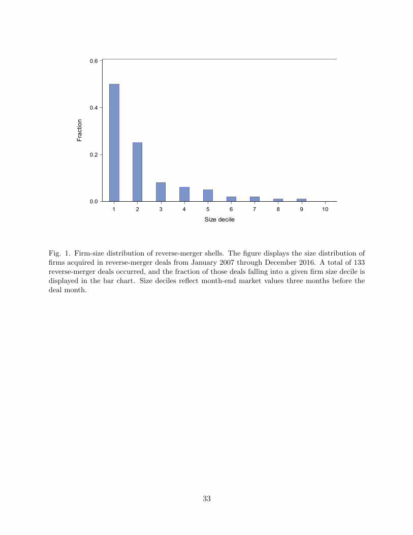
1 2 3 4 5 6 7 8 9 10

Size decile

0.0

0.2

0.4

0.6

Fra

ctio

n

Fig. 1. Firm-size distribution of reverse-merger shells. The figure displays the size distribution offirms acquired in reverse-merger deals from January 2007 through December 2016. A total of 133reverse-merger deals occurred, and the fraction of those deals falling into a given firm size decile isdisplayed in the bar chart. Size deciles reflect month-end market values three months before thedeal month.

33

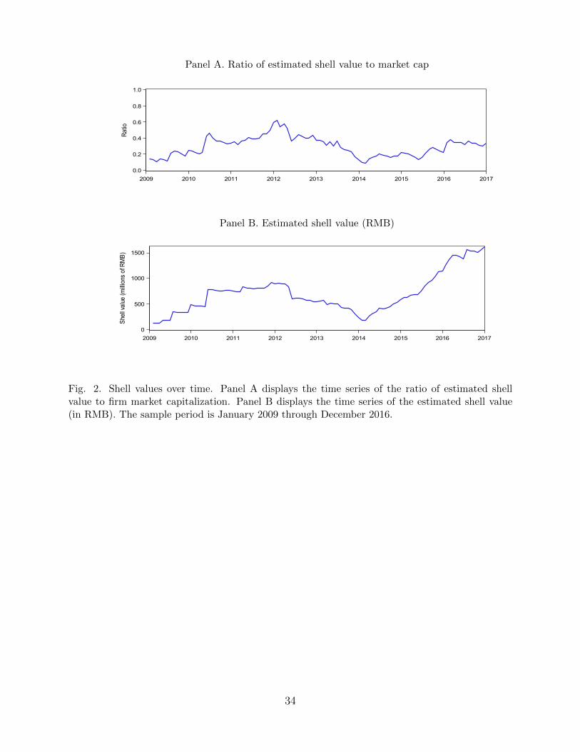
Panel A. Ratio of estimated shell value to market cap

2009 2010 2011 2012 2013 2014 2015 2016 2017

0.0

0.2

0.4

0.6

0.8

1.0

Ratio

Panel B. Estimated shell value (RMB)

2009 2010 2011 2012 2013 2014 2015 2016 2017

0

500

1000

1500

She

ll val

ue (m

illion

s of

RM

B)

Fig. 2. Shell values over time. Panel A displays the time series of the ratio of estimated shellvalue to firm market capitalization. Panel B displays the time series of the estimated shell value(in RMB). The sample period is January 2009 through December 2016.

34

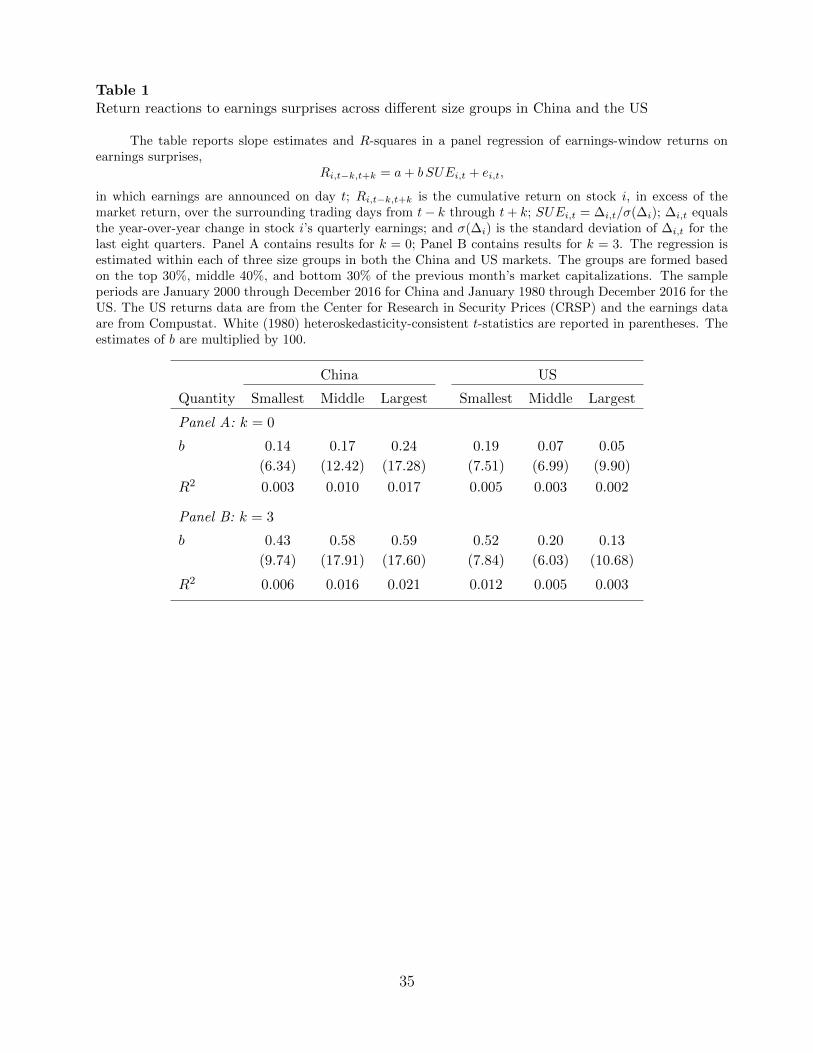
Table 1Return reactions to earnings surprises across different size groups in China and the US

The table reports slope estimates and R-squares in a panel regression of earnings-window returns onearnings surprises,

Ri,t−k,t+k = a+ b SUEi,t + ei,t,

in which earnings are announced on day t; Ri,t−k,t+k is the cumulative return on stock i, in excess of themarket return, over the surrounding trading days from t− k through t+ k; SUEi,t = ∆i,t/σ(∆i); ∆i,t equalsthe year-over-year change in stock i’s quarterly earnings; and σ(∆i) is the standard deviation of ∆i,t for thelast eight quarters. Panel A contains results for k = 0; Panel B contains results for k = 3. The regression isestimated within each of three size groups in both the China and US markets. The groups are formed basedon the top 30%, middle 40%, and bottom 30% of the previous month’s market capitalizations. The sampleperiods are January 2000 through December 2016 for China and January 1980 through December 2016 for theUS. The US returns data are from the Center for Research in Security Prices (CRSP) and the earnings dataare from Compustat. White (1980) heteroskedasticity-consistent t-statistics are reported in parentheses. Theestimates of b are multiplied by 100.

China US

Quantity Smallest Middle Largest Smallest Middle Largest

Panel A: k = 0

b 0.14 0.17 0.24 0.19 0.07 0.05

(6.34) (12.42) (17.28) (7.51) (6.99) (9.90)

R2 0.003 0.010 0.017 0.005 0.003 0.002

Panel B: k = 3

b 0.43 0.58 0.59 0.52 0.20 0.13

(9.74) (17.91) (17.60) (7.84) (6.03) (10.68)

R2 0.006 0.016 0.021 0.012 0.005 0.003

35

Table

2F

ama-

Mac

Bet

hre

gres

sion

sof

stock

retu

rns

onb

eta,

size

,an

dva

luat

ion

rati

os

Th

eta

ble

rep

orts

aver

age

slop

eco

effici

ents

from

mon

th-b

y-m

onth

Fam

a-M

acB

eth

regr

essi

ons.

Ind

ivid

ual

stock

retu

rns

are

regre

ssed

cross

-se

ctio

nal

lyon

stock

char

acte

rist

ics

asof

the

pre

vio

us

mon

th.

Th

eco

lum

ns

corr

esp

ond

tod

iffer

ent

regr

essi

onsp

ecifi

cati

ons,

wit

hn

on

emp

tyro

ws

ind

icat

ing

the

incl

ud

edre

gres

sors

.T

he

regr

esso

rsin

clu

de

pre

ran

kin

gC

AP

Mβt

esti

mat

edu

sin

gth

ep

ast

12m

onth

sof

dai

lyre

turn

sw

ith

afi

ve-l

ag

Dim

son

(197

9)co

rrec

tion

;th

elo

gof

mon

th-e

nd

mar

ket

cap

(logM

);th

elo

gof

book

-to-

mar

ket

(logBM

);th

elo

gof

asse

ts-t

o-m

arke

t(logAM

);EP

+,

wh

ich

equ

als

the

pos

itiv

eva

lues

ofea

rnin

gs-t

o-p

rice

,an

dze

root

her

wis

e;D

(EP<

0),

wh

ich

equ

als

one

ifea

rnin

gsar

en

egat

ive,

and

zero

oth

erw

ise;

CP

+;

andD

(CP<

0)(w

ith

the

last

two

sim

ilar

lyd

efin

ed).

Th

ela

stro

wre

por

tsth

eav

erag

ead

just

edR

-squ

ared

for

each

spec

ifica

tion

.T

he

sam

ple

per

iod

isJan

uar

y20

00th

rou

ghD

ecem

ber

2016

.T

het-

stat

isti

csb

ased

onN

ewey

and

Wes

t(1

987)

stan

dar

der

rors

wit

hfo

ur

lags

are

rep

ort

edin

par

enth

eses

.

Qu

anti

ty(1

)(2

)(3

)(4

)(5

)(6

)(7

)(8

)(9

)

Inte

rcep

t0.

0149

0.05

810.

0571

0.06

590.

0629

0.06

900.0

564

0.0

716

0.0

728

(1.9

4)(3

.32)

(3.1

9)(3

.90)

(3.7

4)(4

.03)

(3.1

9)

(4.4

0)

(4.3

9)

β−

0.00

02−

0.00

10−

0.00

18−

0.00

170.

0002

−0.0

010−

0.0

002−

0.0

004

(−0.

09)

(−0.

37)

(−0.

71)

(−0.

67)

(0.0

7)(−

0.3

7)

(−0.0

6)

(−0.1

5)

logME

−0.

0049

−0.

0046

−0.

0046

−0.

0048

−0.

0068

−0.0

047−

0.0

066−

0.0

064

(−2.

91)

(−2.

69)

(−2.

73)

(−3.

00)

(−4.

34)

(−2.8

0)

(−4.4

9)

(−4.4

0)

logBM

0.00

570.0

022

0.0

035

(3.2

1)(1

.31)

(1.7

6)

logAM

0.00

450.0

014

(3.0

3)(0

.99)

EP

+0.

9503

0.7

825

0.7

960

(4.8

8)(4

.38)

(5.0

6)

D(EP<

0)0.

0006

−0.0

005−

0.0

001

(0.3

1)(−

0.2

9)

(−0.0

4)

CP

+0.0

546

0.0

181

(3.4

1)

(1.3

5)

D(CP<

0)0.0

019

0.0

016

(3.1

1)

(2.3

7)

R2

0.01

960.

0277

0.04

410.

0652

0.06

770.

0615

0.0

454

0.0

832

0.0

776

36

Table 3Summary statistics for the CH-3 factors

This table reports the means, standard deviations, t-statistics, and pairwise correlations for the threefactors in the CH-3 model. The means and standard deviations are expressed in percent per month. Thesample period is January 2000 through December 2016 (204 months).

Correlations

Factor Mean Std. dev. t-stat. MKT SMB VMG

MKT 0.66 8.09 1.16 1.00 0.12 −0.27SMB 1.03 4.52 3.25 0.12 1.00 −0.62VMG 1.14 3.75 4.34 −0.27 −0.62 1.00

37

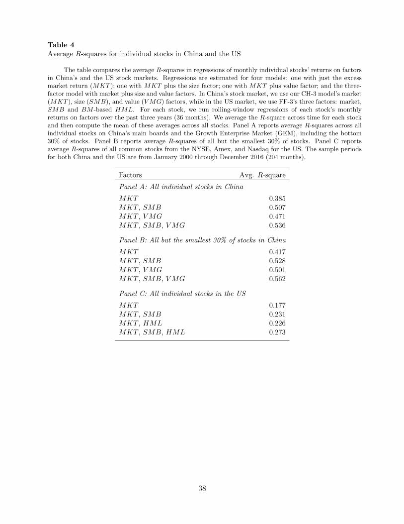
Table 4Average R-squares for individual stocks in China and the US

The table compares the average R-squares in regressions of monthly individual stocks’ returns on factorsin China’s and the US stock markets. Regressions are estimated for four models: one with just the excessmarket return (MKT ); one with MKT plus the size factor; one with MKT plus value factor; and the three-factor model with market plus size and value factors. In China’s stock market, we use our CH-3 model’s market(MKT ), size (SMB), and value (VMG) factors, while in the US market, we use FF-3’s three factors: market,SMB and BM -based HML. For each stock, we run rolling-window regressions of each stock’s monthlyreturns on factors over the past three years (36 months). We average the R-square across time for each stockand then compute the mean of these averages across all stocks. Panel A reports average R-squares across allindividual stocks on China’s main boards and the Growth Enterprise Market (GEM), including the bottom30% of stocks. Panel B reports average R-squares of all but the smallest 30% of stocks. Panel C reportsaverage R-squares of all common stocks from the NYSE, Amex, and Nasdaq for the US. The sample periodsfor both China and the US are from January 2000 through December 2016 (204 months).

Factors Avg. R-square

Panel A: All individual stocks in China

MKT 0.385MKT , SMB 0.507MKT , VMG 0.471MKT , SMB, VMG 0.536

Panel B: All but the smallest 30% of stocks in China

MKT 0.417MKT , SMB 0.528MKT , VMG 0.501MKT , SMB, VMG 0.562

Panel C: All individual stocks in the US

MKT 0.177MKT , SMB 0.231MKT , HML 0.226MKT , SMB, HML 0.273

38

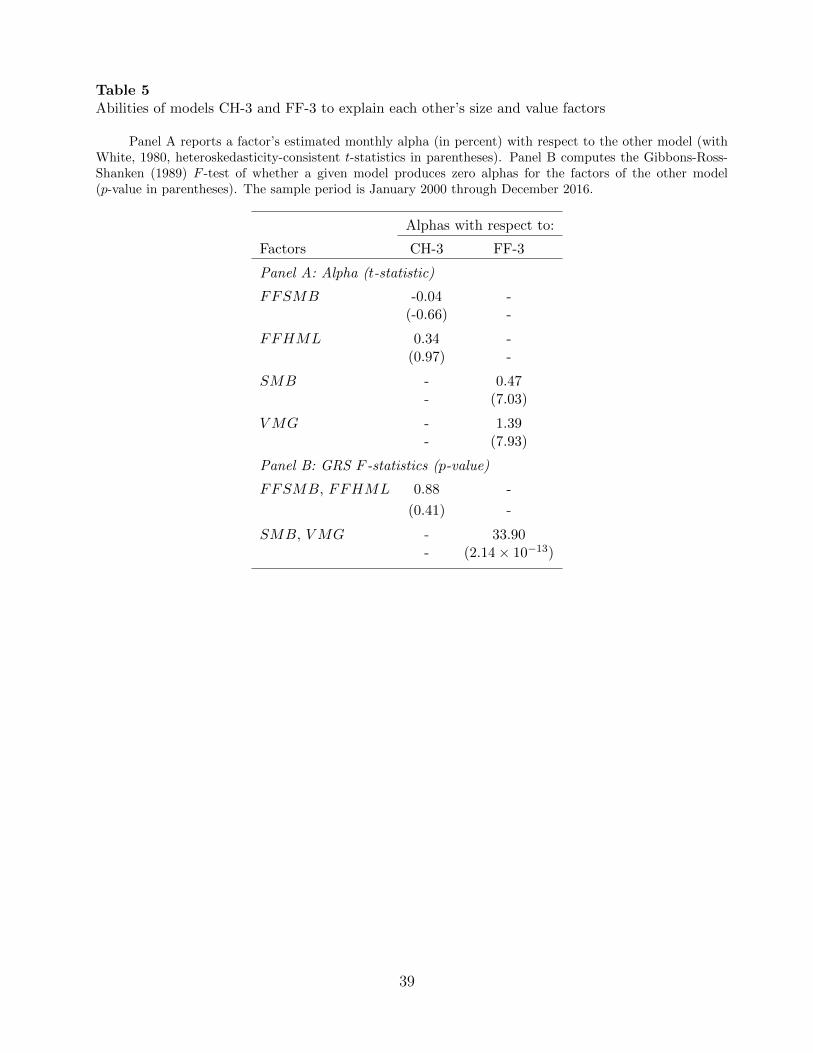
Table 5Abilities of models CH-3 and FF-3 to explain each other’s size and value factors

Panel A reports a factor’s estimated monthly alpha (in percent) with respect to the other model (withWhite, 1980, heteroskedasticity-consistent t-statistics in parentheses). Panel B computes the Gibbons-Ross-Shanken (1989) F -test of whether a given model produces zero alphas for the factors of the other model(p-value in parentheses). The sample period is January 2000 through December 2016.

Alphas with respect to:

Factors CH-3 FF-3

Panel A: Alpha (t-statistic)

FFSMB -0.04 -(-0.66) -

FFHML 0.34 -(0.97) -

SMB - 0.47- (7.03)

VMG - 1.39- (7.93)

Panel B: GRS F -statistics (p-value)

FFSMB, FFHML 0.88 -

(0.41) -

SMB, VMG - 33.90- (2.14× 10−13)

39

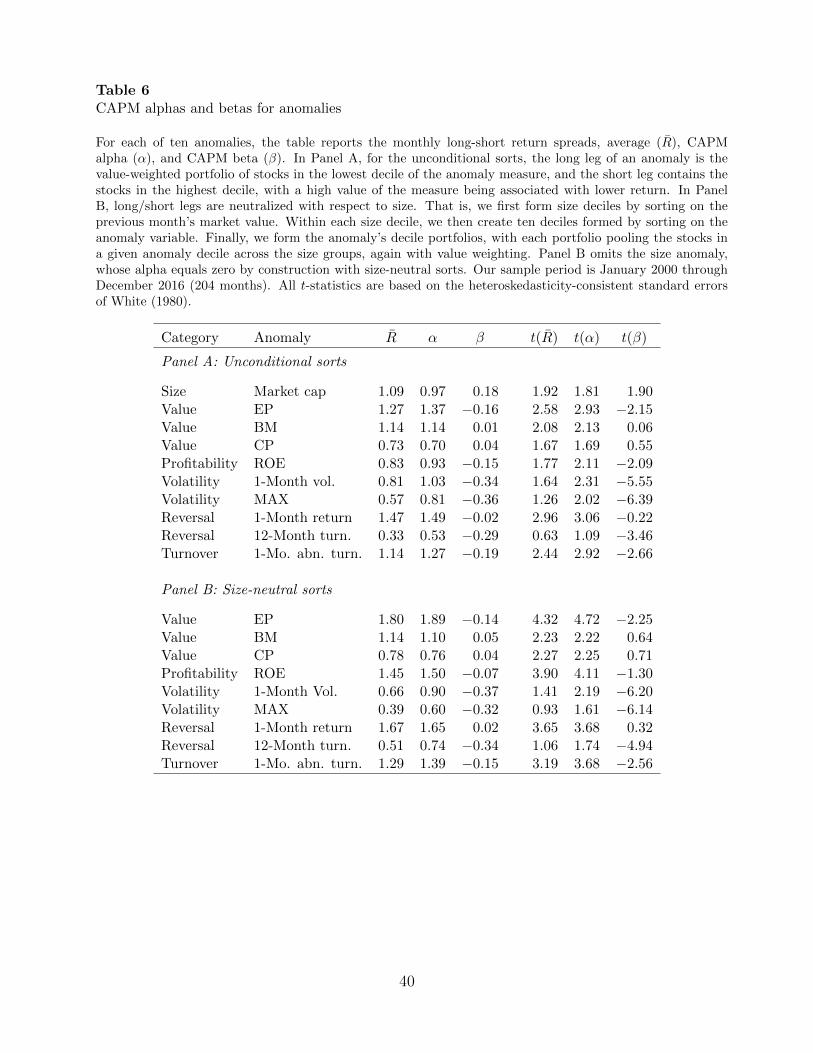
Table 6CAPM alphas and betas for anomalies

For each of ten anomalies, the table reports the monthly long-short return spreads, average (R), CAPMalpha (α), and CAPM beta (β). In Panel A, for the unconditional sorts, the long leg of an anomaly is thevalue-weighted portfolio of stocks in the lowest decile of the anomaly measure, and the short leg contains thestocks in the highest decile, with a high value of the measure being associated with lower return. In PanelB, long/short legs are neutralized with respect to size. That is, we first form size deciles by sorting on theprevious month’s market value. Within each size decile, we then create ten deciles formed by sorting on theanomaly variable. Finally, we form the anomaly’s decile portfolios, with each portfolio pooling the stocks ina given anomaly decile across the size groups, again with value weighting. Panel B omits the size anomaly,whose alpha equals zero by construction with size-neutral sorts. Our sample period is January 2000 throughDecember 2016 (204 months). All t-statistics are based on the heteroskedasticity-consistent standard errorsof White (1980).

Category Anomaly R α β t(R) t(α) t(β)

Panel A: Unconditional sorts

Size Market cap 1.09 0.97 0.18 1.92 1.81 1.90Value EP 1.27 1.37 −0.16 2.58 2.93 −2.15Value BM 1.14 1.14 0.01 2.08 2.13 0.06Value CP 0.73 0.70 0.04 1.67 1.69 0.55Profitability ROE 0.83 0.93 −0.15 1.77 2.11 −2.09Volatility 1-Month vol. 0.81 1.03 −0.34 1.64 2.31 −5.55Volatility MAX 0.57 0.81 −0.36 1.26 2.02 −6.39Reversal 1-Month return 1.47 1.49 −0.02 2.96 3.06 −0.22Reversal 12-Month turn. 0.33 0.53 −0.29 0.63 1.09 −3.46Turnover 1-Mo. abn. turn. 1.14 1.27 −0.19 2.44 2.92 −2.66

Panel B: Size-neutral sorts

Value EP 1.80 1.89 −0.14 4.32 4.72 −2.25Value BM 1.14 1.10 0.05 2.23 2.22 0.64Value CP 0.78 0.76 0.04 2.27 2.25 0.71Profitability ROE 1.45 1.50 −0.07 3.90 4.11 −1.30Volatility 1-Month Vol. 0.66 0.90 −0.37 1.41 2.19 −6.20Volatility MAX 0.39 0.60 −0.32 0.93 1.61 −6.14Reversal 1-Month return 1.67 1.65 0.02 3.65 3.68 0.32Reversal 12-Month turn. 0.51 0.74 −0.34 1.06 1.74 −4.94Turnover 1-Mo. abn. turn. 1.29 1.39 −0.15 3.19 3.68 −2.56

40

Table 7CH-3 alphas and factor loadings for anomalies

For each of ten anomalies, the table reports the monthly long-short return spread’s CH-3 alpha and factor loadings. For eachanomaly, the regression estimated is

Rt = α+ βMKTMKTt + βSMBSMBt + βVMGVMGt + εt,

where Rt is the anomaly’s long-short return spread in month t, MKTt is the excess market return, SMBt is CH-3’s sizefactor, and VMGt is the EP -based value factor. In Panel A, for the unconditional sorts, the long leg of an anomaly is thevalue-weighted portfolio of stocks in the lowest decile of the anomaly measure, and the short leg contains the stocks in thehighest decile, with a high value of the measure being associated with lower return. In Panel B, long/short legs are neutralizedwith respect to size. That is, we first form size deciles by sorting on the previous month’s market value. Within each sizedecile, we then create ten deciles formed by sorting on the anomaly variable. Finally, we form the anomaly’s decile portfolios,with each portfolio pooling the stocks in a given anomaly decile across the size groups, again with value weighting. Panel Bomits the size anomaly, whose alpha equals zero by construction with size-neutral sorts. Our sample period is January 2000through December 2016. All t-statistics are based on the heteroskedasticity-consistent standard errors of White (1980).

Category Anomaly α βMKT βSMB βVMG t(α) t(βMKT ) t(βSMB) t(βVMG)

Panel A: Unconditional sorts

Size Market cap 0.21 0.01 1.45 −0.54 1.71 0.77 40.88 −11.70Value EP 0.04 0.04 −0.38 1.40 0.16 1.31 −4.73 14.75Value BM 0.64 0.06 −0.03 0.43 1.02 0.65 −0.14 1.64Value CP 0.20 0.14 −0.28 0.64 0.45 2.10 −1.95 4.00Profitability ROE −0.36 0.03 −0.29 1.28 −0.88 0.70 −2.35 9.43Volatility 1-Month vol. 0.23 −0.23 −0.12 0.75 0.44 −3.81 −0.67 3.86Volatility MAX 0.27 −0.30 −0.05 0.48 0.65 −4.57 −0.30 2.55Reversal 1-Month return 0.93 −0.06 0.56 0.01 1.70 −0.69 3.15 0.03Turnover 12-Month turn. 0.42 −0.14 −0.85 0.77 1.30 −3.69 −9.33 7.90Turnover 1-Mo. abn. turn. 1.28 −0.22 0.18 −0.16 2.86 −2.78 0.93 −0.76

Panel B: Size-neutral sorts

Value EP 0.23 0.02 0.05 1.32 0.82 0.47 0.57 11.97Value BM 0.61 0.13 −0.15 0.53 0.98 1.60 −0.80 2.19Value CP 0.18 0.11 −0.06 0.52 0.54 1.98 −0.50 3.84Profitability ROE −0.37 0.05 0.41 1.20 −1.04 1.23 4.14 9.66Volatility 1-Month vol. 0.20 −0.28 −0.08 0.64 0.42 −4.96 −0.49 3.34Volatility MAX 0.00 −0.26 0.05 0.45 0.00 −4.38 0.30 2.50Reversal 1-Month return 1.13 0.01 0.41 0.10 2.12 0.11 2.59 0.55Turnover 12-Month turn. 0.25 −0.22 −0.43 0.74 0.69 −4.94 −3.91 5.74Turnover 1-Mo. abn. turn. 1.24 −0.18 0.25 −0.08 3.04 −2.79 1.55 −0.43

41

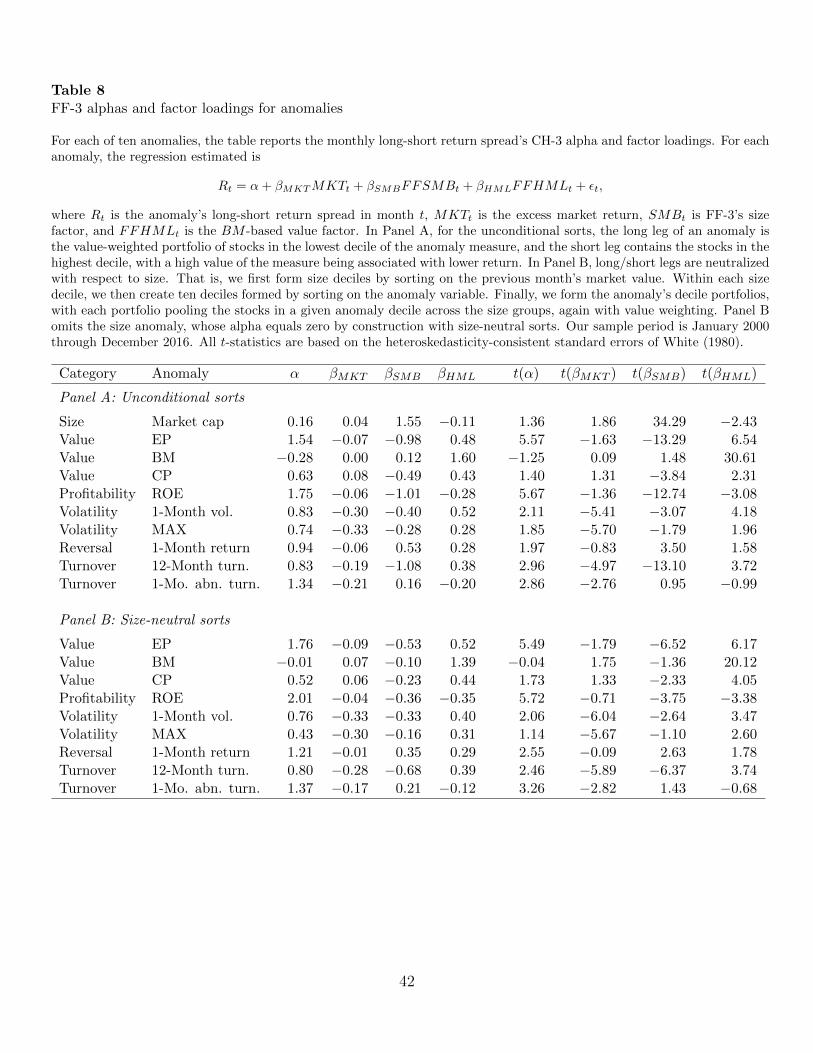
Table 8FF-3 alphas and factor loadings for anomalies

For each of ten anomalies, the table reports the monthly long-short return spread’s CH-3 alpha and factor loadings. For eachanomaly, the regression estimated is

Rt = α+ βMKTMKTt + βSMBFFSMBt + βHMLFFHMLt + εt,

where Rt is the anomaly’s long-short return spread in month t, MKTt is the excess market return, SMBt is FF-3’s sizefactor, and FFHMLt is the BM -based value factor. In Panel A, for the unconditional sorts, the long leg of an anomaly isthe value-weighted portfolio of stocks in the lowest decile of the anomaly measure, and the short leg contains the stocks in thehighest decile, with a high value of the measure being associated with lower return. In Panel B, long/short legs are neutralizedwith respect to size. That is, we first form size deciles by sorting on the previous month’s market value. Within each sizedecile, we then create ten deciles formed by sorting on the anomaly variable. Finally, we form the anomaly’s decile portfolios,with each portfolio pooling the stocks in a given anomaly decile across the size groups, again with value weighting. Panel Bomits the size anomaly, whose alpha equals zero by construction with size-neutral sorts. Our sample period is January 2000through December 2016. All t-statistics are based on the heteroskedasticity-consistent standard errors of White (1980).

Category Anomaly α βMKT βSMB βHML t(α) t(βMKT ) t(βSMB) t(βHML)

Panel A: Unconditional sorts

Size Market cap 0.16 0.04 1.55 −0.11 1.36 1.86 34.29 −2.43Value EP 1.54 −0.07 −0.98 0.48 5.57 −1.63 −13.29 6.54Value BM −0.28 0.00 0.12 1.60 −1.25 0.09 1.48 30.61Value CP 0.63 0.08 −0.49 0.43 1.40 1.31 −3.84 2.31Profitability ROE 1.75 −0.06 −1.01 −0.28 5.67 −1.36 −12.74 −3.08Volatility 1-Month vol. 0.83 −0.30 −0.40 0.52 2.11 −5.41 −3.07 4.18Volatility MAX 0.74 −0.33 −0.28 0.28 1.85 −5.70 −1.79 1.96Reversal 1-Month return 0.94 −0.06 0.53 0.28 1.97 −0.83 3.50 1.58Turnover 12-Month turn. 0.83 −0.19 −1.08 0.38 2.96 −4.97 −13.10 3.72Turnover 1-Mo. abn. turn. 1.34 −0.21 0.16 −0.20 2.86 −2.76 0.95 −0.99

Panel B: Size-neutral sorts

Value EP 1.76 −0.09 −0.53 0.52 5.49 −1.79 −6.52 6.17Value BM −0.01 0.07 −0.10 1.39 −0.04 1.75 −1.36 20.12Value CP 0.52 0.06 −0.23 0.44 1.73 1.33 −2.33 4.05Profitability ROE 2.01 −0.04 −0.36 −0.35 5.72 −0.71 −3.75 −3.38Volatility 1-Month vol. 0.76 −0.33 −0.33 0.40 2.06 −6.04 −2.64 3.47Volatility MAX 0.43 −0.30 −0.16 0.31 1.14 −5.67 −1.10 2.60Reversal 1-Month return 1.21 −0.01 0.35 0.29 2.55 −0.09 2.63 1.78Turnover 12-Month turn. 0.80 −0.28 −0.68 0.39 2.46 −5.89 −6.37 3.74Turnover 1-Mo. abn. turn. 1.37 −0.17 0.21 −0.12 3.26 −2.82 1.43 −0.68

42

Table 9Comparing the abilities of models to explain anomalies

The table reports measures summarizing the degree to which anomalies produce alphas under three differentfactor models: CAPM, FF-3, and CH-3. Also reported are measures for “unadjusted” return spreads (i.e., fora model with no factors). For each model, the table reports the average absolute monthly alpha (in percent),average absolute t-statistic, the Gibbons, Ross, and Shanken (1989) “GRS” F -statistic with associated p-value,and the number of anomalies for which the model produces the smallest absolute alpha among the four models.In Panel A, for the unconditional sorts, the long leg of an anomaly is the value-weighted portfolio of stocks inthe lowest decile of the anomaly measure, and the short leg contains the stocks in the highest decile, with ahigh value of the measure being associated with lower return. In Panel B, long/short legs are neutralized withrespect to size. That is, we first form size deciles by sorting on the previous month’s market value. Withineach size decile, we then create ten deciles formed by sorting on the anomaly variable. Finally, we form theanomaly’s decile portfolios, with each portfolio pooling the stocks in a given anomaly decile across the sizegroups, again with value weighting. Two versions of the GRS test are reported. In Panel A, GRS10 uses all tenanomalies, while GRS7 excludes the anomalies for size, BM , and EP , which are variables used to constructfactors. Panel B omits the size anomaly, whose alpha equals zero by construction with size-neutral sorts. Allt-statistics are based on the heteroskedasticity-consistent standard errors of White (1980). The sample periodis from January 2000 through December 2016 (204 months).

Measure Unadjusted CAPM FF-3 CH-3

Panel A: Unconditional sorts

Average |α| 0.94 1.02 0.90 0.45Average |t| 1.89 2.21 2.70 1.12

GRS10 7.30 7.31 6.00 1.49p10 <0.0001 <0.0001 <0.0001 0.15

GRS7 4.40 4.45 6.86 1.74p7 0.0002 0.0001 0.0001 0.10

Panel B: Size-neutral sorts

Average |α| 1.08 1.17 0.99 0.47Average |t| 2.55 2.91 2.72 1.07

GRS9 8.24 8.08 7.97 1.97p9 <0.0001 <0.0001 <0.0001 0.05

GRS7 8.15 8.10 9.11 2.33p7 <0.0001 <0.0001 <0.0001 0.03

43

Table

10

An

omal

yal

ph

asu

nd

era

fou

r-fa

ctor

mod

el

For

each

ofte

nan

omal

ies,

the

tab

lere

port

sth

em

onth

lylo

ng-

shor

tre

turn

spre

ad’s

CH

-4al

ph

aan

dfa

ctor

load

ings

.F

orea

chan

omal

y,th

ere

gre

ssio

nes

tim

ated

isR

t=α

+βM

KTMKTt

+βSM

BSMB

t+βVM

GVMG

t+βPM

OPMO

t+ε t,

inw

hic

hR

tis

the

anom

aly’s

lon

g-s

hor

tre

turn

spre

adin

mon

tht,MKTt

isth

eex

cess

mar

ket

retu

rn,SMB

tis

CH

-3’s

size

fact

or,VMG

tis

theEP

-b

ased

valu

efa

ctor

,an

dPMO

t(p

essi

mis

tic

min

us

opti

mis

tic)

isth

ese

nti

men

tfa

ctor

bas

edon

abn

orm

altu

rnov

er.

InP

anel

A,

for

the

un

con

dit

ion

al

sort

s,th

elo

ng

leg

ofan

anom

aly

isth

eva

lue-

wei

ghte

dp

ortf

olio

ofst

ock

sin

the

low

est

dec

ile

ofth

ean

omal

ym

easu

re,

and

the

shor

tle

gco

nta

ins

the

stock

sin

the

hig

hes

td

ecil

e,w

ith

ah

igh

valu

eof

the

mea

sure

bei

ng

asso

ciat

edw

ith

low

erre

turn

.In

Pan

elB

,lo

ng/

shor

tle

gsar

en

eutr

ali

zed

wit

hre

spec

tto

size

.T

hat

is,

we

firs

tfo

rmsi

zedec

iles

by

sort

ing

onth

ep

revio

us

mon

th’s

mar

ket

valu

e.W

ith

inea

chsi

zed

ecil

e,w

eth

encr

eate

ten

dec

iles

form

edby

sort

ing

onth

ean

omal

yva

riab

le.

Fin

ally

,w

efo

rmth

ean

omal

y’s

dec

ile

por

tfol

ios,

wit

hea

chp

ortf

olio

pool

ing

the

stock

sin

agiv

enan

om

aly

dec

ile

acro

ssth

esi

zegr

oup

s,ag

ain

wit

hva

lue

wei

ghti

ng.

Pan

elB

omit

sth

esi

zean

omal

y,w

hos

eal

ph

aeq

ual

sze

roby

con

stru

ctio

nw

ith

size

-neu

tral

sort

s.O

ur

sam

ple

per

iod

isJan

uar

y20

00th

rou

ghD

ecem

ber

2016

.A

llt-

stat

isti

csar

eb

ased

onth

eh

eter

oske

das

tici

ty-c

onsi

sten

tst

and

ard

erro

rsof

Wh

ite

(198

0).

Cat

egor

yA

nom

aly

αβMKT

βSMB

βVMG

βPMO

t(α

)t(βMKT

)t(βSMB

)t(βVMG

)t(βPMO

)

Panel

A:Unconditionalsorts

Siz

eM

arke

tca

p0.

23

0.05

1.50

−0.

420.

011.

413.0

539.3

8−

6.8

80.1

7V

alu

eE

P0.

020.

00−

0.46

1.34

0.04

0.08

0.0

7−

5.3

813.1

50.3

3V

alu

eB

M0.

750.

03−

0.02

0.43

−0.

131.

040.3

2−

0.0

91.5

5−

0.4

5V

alu

eC

P0.

310.

09−

0.26

0.65

−0.

200.

571.4

3−

1.8

13.6

0−

1.1

0P

rofi

tab

ilit

yR

OE

−0.

29−

0.03

−0.

361.

28−

0.10

−0.

68−

0.7

0−

3.2

18.7

4−

0.9

6V

olat

ilit

y1-

Mon

thvo

l.−

0.27

−0.

16−

0.27

0.59

0.72

−0.

51−

2.7

1−

1.8

53.2

75.1

3V

olat

ilit

yM

AX

−0.

59−

0.18

−0.

130.

440.

88−

1.64

−3.0

7−

0.9

02.9

17.9

1R

ever

sal

1-M

onth

retu

rn0.

490.

020.

540.

040.

460.

870.2

93.1

90.1

82.4

8T

urn

over

12-M

onth

turn

.0.

04−

0.11

−0.

940.

640.

430.

11−

3.3

6−

10.6

05.0

93.6

9T

urn

over

1-M

o.ab

n.

turn

.−

0.00

−0.

010.

07−

0.27

1.44

−0.

01−

0.3

20.6

8−

2.4

316.4

7

Panel

B:Size-neutralsorts

Val

ue

EP

0.43

−0.

04−

0.03

1.28

−0.

121.

42−

0.7

9−

0.3

511.7

4−

1.0

9V

alu

eB

M0.

570.

12−

0.18

0.46

0.09

0.82

1.5

8−

1.0

41.8

30.3

9V

alu

eC

P0.

190.

08−

0.03

0.57

−0.

120.

491.5

6−

0.2

63.6

7−

0.9

2P

rofi

tab

ilit

yR

OE

−0.

300.

020.

351.

23−

0.05

−0.

760.5

13.6

78.9

9−

0.4

0V

olat

ilit

y1-

Mon

thvo

l.−

0.27

−0.

21−

0.20

0.51

0.63

−0.

59−

3.9

5−

1.3

72.8

74.9

0V

olat

ilit

yM

AX

−0.

77−

0.17

0.00

0.45

0.74

−2.

05−

2.8

60.0

12.9

55.8

1R

ever

sal

1-M

onth

retu

rn0.

710.

070.

400.

120.

421.

281.1

42.6

20.6

82.6

0T

urn

over

12-M

onth

turn

.−

0.07

−0.

19−

0.53

0.61

0.44

−0.

19−

4.1

6−

4.3

83.7

73.3

9T

urn

over

1-M

o.ab

n.

turn

.0.

17−

0.00

0.17

−0.

171.

210.

67−

0.0

51.8

3−

1.9

015.2

3

44

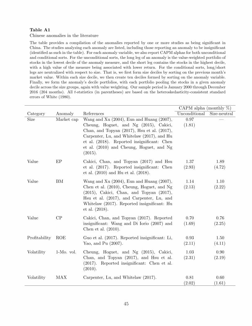
Table A1Chinese anomalies in the literature

The table provides a compilation of the anomalies reported by one or more studies as being significant inChina. The studies analyzing each anomaly are listed, including those reporting an anomaly to be insignificant(identified as such in the table). For each anomaly variable, we also report CAPM alphas for both unconditionaland conditional sorts. For the unconditional sorts, the long leg of an anomaly is the value-weighted portfolio ofstocks in the lowest decile of the anomaly measure, and the short leg contains the stocks in the highest decile,with a high value of the measure being associated with lower return. For the conditional sorts, long/shortlegs are neutralized with respect to size. That is, we first form size deciles by sorting on the previous month’smarket value. Within each size decile, we then create ten deciles formed by sorting on the anomaly variable.Finally, we form the anomaly’s decile portfolios, with each portfolio pooling the stocks in a given anomalydecile across the size groups, again with value weighting. Our sample period is January 2000 through December2016 (204 months). All t-statistics (in parentheses) are based on the heteroskedasticity-consistent standarderrors of White (1980).

CAPM alpha (monthly %)Category Anomaly References Unconditional Size-neutral

Size Market cap Wang and Xu (2004), Eun and Huang (2007),Cheung, Hoguet, and Ng (2015), Cakici,Chan, and Topyan (2017), Hsu et al. (2017),Carpenter, Lu, and Whitelaw (2017), and Huet al. (2018). Reported insignificant: Chenet al. (2010) and Cheung, Hoguet, and Ng(2015).

0.97(1.81)

—

Value EP Cakici, Chan, and Topyan (2017) and Hsuet al. (2017). Reported insignificant: Chenet al. (2010) and Hu et al. (2018).

1.37(2.93)

1.89(4.72)

Value BM Wang and Xu (2004), Eun and Huang (2007),Chen et al. (2010), Cheung, Hoguet, and Ng(2015), Cakici, Chan, and Topyan (2017),Hsu et al. (2017), and Carpenter, Lu, andWhitelaw (2017). Reported insignificant: Huet al. (2018).

1.14(2.13)

1.10(2.22)

Value CP Cakici, Chan, and Topyan (2017). Reportedinsignificant: Wang and Di Iorio (2007) andChen et al. (2010).

0.70(1.69)

0.76(2.25)

Profitability ROE Guo et al. (2017). Reported insignificant: Li,Yao, and Pu (2007).

0.93(2.11)

1.50(4.11)

Volatility 1-Mo. vol. Cheung, Hoguet, and Ng (2015), Cakici,Chan, and Topyan (2017), and Hsu et al.(2017). Reported insignificant: Chen et al.(2010).

1.03(2.31)

0.90(2.19)

Volatility MAX Carpenter, Lu, and Whitelaw (2017). 0.81(2.02)

0.60(1.61)

45

Table A1Chinese anomalies in the literature (continued)

CAPM alpha (monthly %)Category Anomaly References Unconditional Size-neutral

Reversal 1-Month return Cakici, Chan, and Topyan (2017), Hsu et al.(2017), and Carpenter, Lu, and Whitelaw(2017). Reported insignificant: Cheung,Hoguet, and Ng (2015).

1.49(3.06)

1.65(3.68)

Turnover 12-Month turn. Zhang and Liu (2006) and Eun and Huang(2007). Reported insignificant: Chen et al.(2010).

0.53(1.09)

0.74(1.74)

Turnover 1-Mo. abn. turn. Li and Wu (2003) and Zhang and Liu (2006). 1.27(2.92)

1.39(3.68)

Investment Asset growth Chen et al. (2010). Reported insignificant:Hsu et al. (2017), Guo et al. (2017), and Lin(2017).

0.22(0.72)

−0.05(−0.20)

Accruals Accruals Li et al. (2011) and Hsu et al. (2017). Re-ported insignificant: Chen et al. (2010).

0.08(0.39)

−0.15(−0.70)

Accruals NOA Chen et al. (2010) and Hsu et al. (2017). 0.38(1.03)

0.42(1.22)

Illiquidity Amihud illiq. Carpenter, Lu, and Whitelaw (2017) andChen et al. (2010).

0.83(1.62)

0.63(1.55)

46

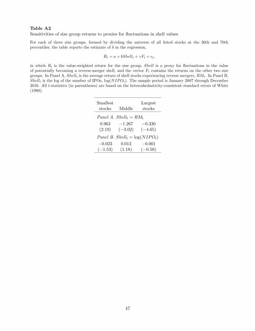
Table A2Sensitivities of size group returns to proxies for fluctuations in shell values

For each of three size groups, formed by dividing the universe of all listed stocks at the 30th and 70thpercentiles, the table reports the estimate of b in the regression,

Rt = a+ bShellt + γFt + εt,

in which Rt is the value-weighted return for the size group, Shell is a proxy for fluctuations in the valueof potentially becoming a reverse-merger shell, and the vector Ft contains the returns on the other two sizegroups. In Panel A, Shellt is the average return of shell stocks experiencing reverse mergers, RMt. In Panel B,Shellt is the log of the number of IPOs, log(NIPOt). The sample period is January 2007 through December2016. All t-statistics (in parentheses) are based on the heteroskedasticity-consistent standard errors of White(1980).

Smallest Largeststocks Middle stocks

Panel A. Shellt = RMt

0.963 −1.267 −0.330(2.19) (−3.02) (−4.65)

Panel B. Shellt = log(NIPOt)

−0.023 0.013 −0.001(−1.53) (1.18) (−0.50)

47

Table

A3

Fam

a-M

acB

eth

regr

essi

ons

ofst

ock

retu

rns

onb

eta,

size

,an

dva

luat

ion

rati

os;

non

fin

anci

alfirm

s

Th

eta

ble

rep

orts

aver

age

slop

eco

effici

ents

from

mon

th-b

y-m

onth

Fam

a-M

acB

eth

regr

essi

ons

usi

ng

non

fin

anci

alfi

rms.

Ind

ivid

ual

stock

retu

rns

are

regr

esse

dcr

oss-

sect

ion

ally

onst

ock

char

acte

rist

ics

asof

the

pre

vio

us

mon

th.

Th

eco

lum

ns

corr

esp

ond

tod

iffer

ent

regr

essi

onsp

ecifi

cati

ons,

wit

hn

onem

pty

row

sin

dic

atin

gth

ein

clu

ded

regr

esso

rs.

Th

ere

gres

sors

incl

ud

ep

rera

nkin

gC

AP

Mβt

esti

mat

edu

sin

gth

ep

ast

12m

onth

sof

daily

retu

rns

wit

ha

five

-lag

Dim

son

(197

9)co

rrec

tion

;th

elo

gof

mon

th-e

nd

mar

ket

cap

(logM

);th

elo

gof

book

-to-

mar

ket

(logBM

);th

elo

gof

asse

ts-t

o-m

ark

et(logAM

);EP

+,

wh

ich

equ

als

the

pos

itiv

eva

lues

ofea

rnin

gs-t

o-pri

ce,

and

zero

oth

erw

ise;D

(EP<

0),

wh

ich

equ

als

one

ifea

rnin

gsar

en

egati

ve,

an

dze

root

her

wis

e;CP

+;

an

dD

(CP<

0)(w

ith

the

last

two

sim

ilar

lyd

efin

ed).

Th

ela

stro

wre

por

tsth

eav

erag

ead

just

edR

-squ

ared

for

each

spec

ifica

tion

.T

he

sam

ple

per

iod

isJanuar

y200

0th

rou

ghD

ecem

ber

2016

.T

het-

stat

isti

csb

ased

onN

ewey

and

Wes

t(1

987)

stan

dar

der

rors

wit

hfo

ur

lags

are

rep

orte

din

par

enth

eses

.

Qu

anti

ty(1

)(2

)(3

)(4

)(5

)(6

)(7

)(8

)(9

)

Inte

rcep

t0.

0134

0.06

460.

0610

0.06

930.

0642

0.07

140.0

602

0.0

722

0.0

750

(1.7

8)(3

.69)

(3.4

0)(4

.08)

(3.7

9)(4

.16)

(3.3

9)

(4.4

1)

(4.5

1)

β0.

0010

0.00

03−

0.00

06−

0.00

040.

0014

0.0

002

0.0

007

0.0

008

(0.3

4)(0

.09)

(−0.

23)

(−0.

17)

(0.4

9)(0

.09)

(0.2

6)

(0.3

1)

logME

−0.

005

6−

0.00

52−

0.00

51−

0.00

51−

0.00

72−

0.0

053−

0.0

068−

0.0

069

(−3.

37)

(−3.

04)

(−3.

07)

(−3.

14)

(−4.

64)

(−3.0

9)

(−4.4

8)

(−4.4

4)

logBM

0.00

530.0

017

0.0

032

(2.7

9)(0

.96)

(1.7

6)

logAM

0.00

410.0

015

(2.5

5)(0

.94)

EP

+1.

0123

0.8

555

0.8

572

(4.7

8)(4

.51)

(4.5

1)

D(EP<

0)0.

0001

−0.0

012−

0.0

007

(0.0

3)(−

0.6

8)

(−0.3

6)

CP

+0.0

391

0.0

122

(2.2

6)

(0.7

9)

D(CP<

0)0.0

009

0.0

009

(1.3

1)

(1.2

0)

R2

0.01

930.

026

40.

0429

0.06

430.

0660

0.06

150.0

434

0.0

825

0.0

776

48

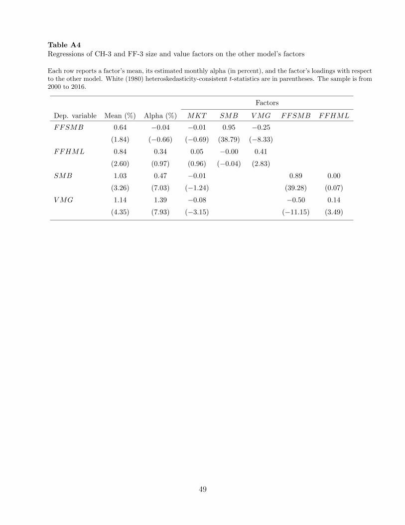
Table A4Regressions of CH-3 and FF-3 size and value factors on the other model’s factors

Each row reports a factor’s mean, its estimated monthly alpha (in percent), and the factor’s loadings with respectto the other model. White (1980) heteroskedasticity-consistent t-statistics are in parentheses. The sample is from2000 to 2016.

Factors

Dep. variable Mean (%) Alpha (%) MKT SMB VMG FFSMB FFHML

FFSMB 0.64 −0.04 −0.01 0.95 −0.25

(1.84) (−0.66) (−0.69) (38.79) (−8.33)

FFHML 0.84 0.34 0.05 −0.00 0.41

(2.60) (0.97) (0.96) (−0.04) (2.83)

SMB 1.03 0.47 −0.01 0.89 0.00

(3.26) (7.03) (−1.24) (39.28) (0.07)

VMG 1.14 1.39 −0.08 −0.50 0.14

(4.35) (7.93) (−3.15) (−11.15) (3.49)

49

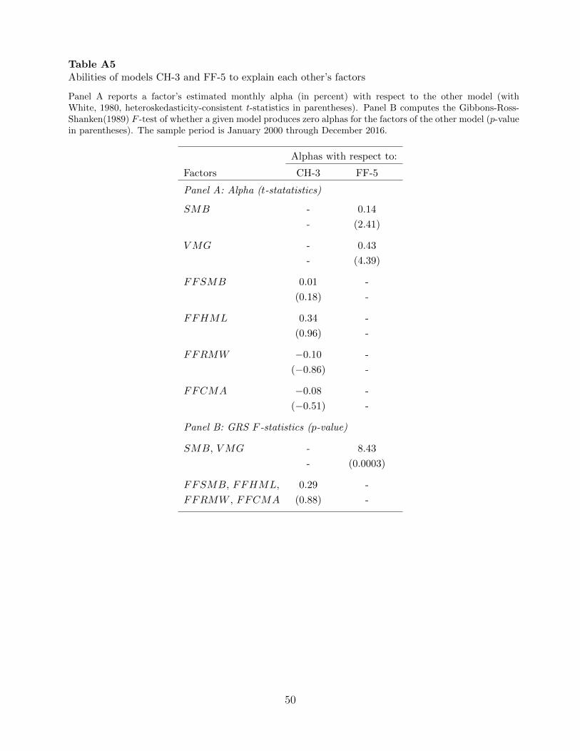
Table A5Abilities of models CH-3 and FF-5 to explain each other’s factors

Panel A reports a factor’s estimated monthly alpha (in percent) with respect to the other model (withWhite, 1980, heteroskedasticity-consistent t-statistics in parentheses). Panel B computes the Gibbons-Ross-Shanken(1989) F -test of whether a given model produces zero alphas for the factors of the other model (p-valuein parentheses). The sample period is January 2000 through December 2016.

Alphas with respect to:

Factors CH-3 FF-5

Panel A: Alpha (t-statatistics)

SMB - 0.14

- (2.41)

VMG - 0.43

- (4.39)

FFSMB 0.01 -

(0.18) -

FFHML 0.34 -

(0.96) -

FFRMW −0.10 -

(−0.86) -

FFCMA −0.08 -

(−0.51) -

Panel B: GRS F -statistics (p-value)

SMB, VMG - 8.43

- (0.0003)

FFSMB, FFHML, 0.29 -

FFRMW , FFCMA (0.88) -

50

1 1.2 1.4 1.6 1.8 2

0

0.1

0.2

0.3

0.4

0.5

0.6

0.7

0.8

0.9

1

FF-3CH-3

Fig. A.1. Model probabilities comparing model CH-3 to model FF-3. The figure displays Bayesianposterior model probabilities for the two-way model comparison. The value on the horizontal axisis the square root of the prior expected maximum Sharpe ratio achievable by combining the model’sfactors, divided by the observed Sharpe ratio of the market. Prior model probabilities are equal.The sample period is from January 2000 through December 2016 (204 months).

51

References

Allen, F., Qian, J., Qian, M., 2003. Comparing China’ s financial system. China Journal ofFinance 1, 1–28.

Allen, F., Qian, J., Qian, M., 2005. Law, finance, and economic growth in China. Journal ofFinancial Economics 77, 57–116.

Allen, F., Qian, J., Qian, M., Zhao, M., 2009. A review of China’s financial system andinitiatives for the future. In: Barth, J.R., Tatom, J. A., Yago, G.(Eds.). China’s emergingfinancial markets: Challenges and Opportunities., Springer, Boston, MA, pp. 3–72.

Allen, F., Qian, J., Shan, C., Zhao, M., 2014. The IPO of industrial and commercial bankof China and the “Chinese Model” of privatizing large financial institutions. EuropeanJournal of Finance 20, 599–624.

Amihud, Y., 2002. Illiquidity and stock returns: cross-section and time-series effects. Journalof Financial Markets 5, 31–56.

Baker, M., Stein, J. C., 2004. Market liquidity as a sentiment indicator. Journal of FinancialMarkets 7, 271–299.

Baker, M., Wurgler, J., 2006. Investor sentiment and the cross-section of stock returns.Journal of Finance 61, 1645–1680.

Ball, R., 1992. The earnings-price anomaly. Journal of Accounting and Economics 15, 319–345.

Banz, R. W., 1981. The relationship between return and market value of common stocks.Journal of Financial Economics 9, 3–18.

Barillas, F., Shanken, J., 2018. Comparing asset pricing models. Journal of Finance 73,715–753.

Basu, S., 1983. The relationship between earnings’ yield, market value and return for NYSEcommon stocks: further evidence. Journal of Financial Economics 12, 129–156.

Bian, J., Da, Z., Lou, D., Zhou, H., 2017. Leverage network and market contagion. Unpub-lished working paper. University of International Business and Economics, University ofNotre Dame, London School of Economics, and Tsinghua University.

Brunnermeier, M. K., Sockin, M., Xiong, W., 2017. China’s model of managing the finan-cial system. Unpublished working paper. Princeton University and University of Texas atAustin.

Cakici, N., Chan, K., Topyan, K., 2017. Cross-sectional stock return predictability in China.European Journal of Finance 23, 581–605.

Campbell, J. Y., Lettau, M., Malkiel, B. G., Xu, Y., 2001. Have individual stocks becomemore volatile? An empirical exploration of idiosyncratic risk. Journal of Finance 56, 1–43.

52

Carhart, M. M., 1997. On persistence in mutual fund performance. Journal of Finance 52,57.

Carpenter, J. N., Lu, F., Whitelaw, R. F., 2017. The real value of China’s stock market.Unpublished working paper.

Carpenter, J. N., Whitelaw, R. F., 2017. The development of China’s stock market andstakes for the global economy. Annual Review of Financial Economics 9, 233–57.

Chen, X., Kim, K. A., Yao, T., Yu, T., 2010. On the predictability of Chinese stock returns.Pacific-Basin Finance Journal 18, 403–425.

Cheung, C., Hoguet, G., Ng, S., 2015. Value, size, momentum, dividend yield, and volatilityin China’s A-share market. Journal of Portfolio Management 41, 57–70.

Dimson, E., 1979. Risk measurement when shares are subject to infrequent trading. Journalof Financial Economics 7, 197–226.

Eun, C. S., Huang, W., 2007. Asset pricing in China’s domestic stock markets: is there alogic? Pacific-Basin Finance Journal 15, 452–480.

Fama, E. F., French, K. R., 1992. The cross-section of expected stock returns. Journal ofFinance 47, 427–465.

Fama, E. F., French, K. R., 1993. Common risk factors in the returns on stocks and bonds.Journal of Financial Economics 33, 3–56.

Fama, E. F., French, K. R., 2015. A five-factor asset pricing model. Journal of FinancialEconomics 116, 1–22.

Fama, E. F., MacBeth, J. D., 1973. Risk, return, and equilibrium: empirical tests. Journalof Political Economy 81, 607–636.

Fan, L., Shan, Y., 2004. Trading volume, valuation ratio, momentum, and a three-factormodel (Translated from Mandarin). Journal of Management Science 7, 13–22.

Floros, I. V., Sapp, T. R. A., 2011. Shell games: on the value of shell companies. Journal ofCorporate Finance 17, 850–867.

Gibbons, M. R., Ross, S. A., Shanken, J., 1989. A test of the efficiency of a given portfolio.Econometrica: Journal of the Econometric Society 57, 1121–1152.

Guo, B., Zhang, W., Zhang, Y., Zhang, H., 2017. The five-factor asset pricing model testsfor the Chinese stockmarket. Pacific-Basin Finance Journal 43, 84–106.

Hirshleifer, D., Hou, K., Teoh, S., Zhang, Y., 2004. Do investors overvalue firms with bloatedbalance sheets? Journal of Accounting and Economics 38, 297–331.

Hou, K., Xue, C., Zhang, L., 2015. Digesting anomalies: an investment approach. Review ofFinancial Studies 28, 650–705.

53

Hsu, J. C., Viswanathan, V., Wang, C., Wool, P., 2017. Anomalies in Chinese A-shares.Unpublished working paper. University of California, Los Angeles and Rayliant GlobalAdvisors.

Hu, G. X., Chen, C., Shao, Y., Wang, J., 2018. Fama–French in China: size and value factorsin Chinese stock returns. International Review of Finance, forthcoming.

Jiang, J., Qian, K., Gong, F., 2016. Institutional holdings’ structure analysis in China (Trans-lated from Mandarin). Unpublished working paper. Shenwan Hongyuan Research, Co.

Lee, C., Qu, Y., Shen, T., 2017. Reverse mergers, shell value, and regulation risk in Chineseequity markets. Unpublished working paper. Stanford University and Tsinghua University.

Lee, E., 2013. Individual stock investor sentiment, stock issuance, and financial marketanomalies. Unpublished working paper. University of Pennsylvania.

Li, Y., Niu, J., Zhang, R., Largay, J. A., 2011. Earnings management and the accrualanomaly: evidence from China. Journal of International Financial Management and Ac-counting 22, 205–245.

Li, Y., Wu, S., 2003. An empirical analysis of the liquidity premium in China (Translatedfrom Mandarin). Management Review 11, 34–42.

Li, Z., Yao, Z., Pu, J., 2007. What are the economics of ROE in China’s stock market?(Translated from Mandarin). Chinese Accounting Review 3, 305–314.

Lin, Q., 2017. Noisy prices and the Fama-French five-factor asset pricing model in China.Emerging Markets Review 31, 141–163.

Newey, W. K., West, K. D., 1987. A simple positive-definite heteroskedasticity andautocorrelation-consistent covariance matrix. Econometrica 55, 703–708.

Niederhoffer, V., Osborne, M. F. M., 1966. Market making and reversal on the stock ex-change. Journal of the American Statistical Association 61, 897–916.

Pastor, L., Stambaugh, R. F., 2000. Comparing asset pricing models: an investment per-spective. Journal of Financial Economics 56, 335–381.

Pastor, L., Stambaugh, R. F., 2003. Liquidity risk and expected stock returns. Journal ofPolitical Economy 111, 642–685.

Ross, S. A., 2017. Factors—theory, statistics, and practice. Journal of Portfolio Management43, 1–5.

Sloan, R. G., 1996. Do stock prices fully reflect information in accruals and cash flows aboutfuture earnings? Accounting Review 71, 289–315.

Song, Z., Xiong, W., 2018. Risks in china’s financial system. Annual Review of FinancialEconomics 10, 261–286.

54

Stambaugh, R. F., Yuan, Y., 2017. Mispricing factors. Review of Financial Studies 30, 1270–1315.

Wang, C., Chin, S., 2004. Profitability of return and volume-based investment strategies inChina’s stock market. Pacific-Basin Finance Journal 12, 541–564.

Wang, F., Xu, Y., 2004. What determines Chinese stock returns? Financial Analysts Journal60, 65–77.

Wang, Y., Di Iorio, A., 2007. The cross-section of expected stock returns in the ChineseA-share market. Global Finance Journal 17, 335–349.

White, H., 1980. A heteroskedasticity-consistent covariance matrix and a direct test forheteroskedasticity. Econometrica 48, 817–838.

Yang, X., Chen, Z., 2003. An empirical analysis of the three-factor model in China (Trans-lated from Mandarin). Quantitative Economics Review 12, 137–141.

Zhang, Z., Liu, L., 2006. The turnover premium: is it a liquidity premium or a bubble?(Translated from Mandarin). Quarterly Economics Journal 3, 871–892.

55