Size bias, sampling, the waiting time paradox,and infinite divisibility: when is the increment

independent?

Richard Arratia, Larry Goldstein

November 20, 2009

Abstract

With X∗ denoting a random variable with the X-size bias distri-bution, what are all distributions for X such that it is possible to haveX∗ = X+Y , Y ≥ 0, with X and Y independent? We give the answer,due to Steutel [17], and also discuss the relations of size biasing to thewaiting time paradox, renewal theory, sampling, tightness and uniformintegrability, compound Poisson distributions, infinite divisibility, andthe lognormal distributions.

1 The Waiting Time Paradox

Here is the “waiting time paradox,” paraphrased from Feller [9], vol-ume II, section I.4: Buses arrive in accordance with a Poisson process,so that the interarrival times are given by independent random vari-ables, having the exponential distribution IP(X > s) = e−s for s > 0,with mean IEX = 1. I now arrive at an arbitrary time t. What isthe expectation IEWt of my waiting time Wt for the next bus? Twocontradictory answers stand to reason: (a) The lack of memory of theexponential distribution, i.e. the property IP(X > r + s|X > s) =IP(X > r), implies that IEWt should not be sensitive to the choice t,so that IEWt = IEW0 = 1. (b) The time of my arrival is “chosen

1

at random” in the interval between two consecutive buses, and forreasons of symmetry IEWt = 1/2.

The resolution of this paradox requires an understanding of sizebiasing. We will first present some simpler examples of size biasing,before returning to the waiting time paradox and its resolution.

Size biasing occurs in many unexpected contexts, such as statis-tical estimation, renewal theory, infinite divisibility of distributions,and number theory. The key relation is that to size bias a sum withindependent summands, one needs only size bias a single summand,chosen at random.

2 Size Biasing in Sampling

We asked students who ate lunch in the cafeteria “How many peo-ple, including yourself, sat at your table?” Twenty percent said theyate alone, thirty percent said they ate with one other person, thirtypercent said they ate at a table of three, and the remaining twentypercent said they ate at a table of four. From this information, wouldit be correct to conclude that twenty percent of the tables had onlyone person, thirty percent had two people, thirty percent had threepeople, and twenty percent had four people?

Certainly not! The easiest way to think about this situation isto imagine 100 students went to lunch, and we interviewed them all.Thus, twenty students ate alone, using 20 tables, thirty students atein pairs, using 15 tables, thirty students ate in trios, using 10 tables,and twenty students ate in groups of four, using 5 tables. So therewere 20 + 15 + 10 + 5 = 50 occupied tables, of which forty percent hadonly one person, thirty percent had two people, twenty percent hadthree people, and ten percent had four people.

A probabilistic view of this example begins by considering the ex-periment where an occupied table is selected at random and the num-ber of people, X, at that table is recorded. From the analysis sofar, we see that since 20 of the 50 occupied tables had only a singleindividual, IP(X = 1) = .4, and so forth. A different experiment,one related to but not to be confused with the first, would be toselect a person at random, and record the total number X∗ at thetable where this individual had lunch. Our story began with the in-formation IP(X∗ = 1) = .2, IP(X∗ = 2) = .3, and so forth, and thedistributions of the random variables X and X∗ are given side by side

2

in the following table:

k IP(X = k) IP(X∗ = k)

1 .4 .22 .3 .33 .2 .34 .1 .2

1.0 1.0

The distributions of the random variables X and X∗ are related; for Xeach table has the same chance to be selected, but for X∗ the chance toselect a table is proportional to the number of people who sat there.Thus IP(X∗ = k) is proportional to k × IP(X = k); expressing theproportionality with a constant c we have IP(X∗ = k) = c×IP(X = k).Since 1 =

∑k IP(X∗ = k) = c

∑k kIP(X = k) = cIEX, we have

c = 1/IEX and

IP(X∗ = k) =kIP(X = k)

IEX; k = 0, 1, 2, . . . . (1)

Since the distribution of X∗ is weighted by the value, or size, of X,we say that X∗ has the X size biased distribution.

In many statistical sampling situations, like the one above, caremust be taken so that one does not inadvertently sample from the sizebiased distribution in place of the one intended. For instance, supposewe wanted to have information on how many voice telephone linesare connected at residential addresses. Calling residential telephonenumbers by random digit dialing and asking how many telephone linesare connected at the locations which respond is an instance where onewould be observing the size biased distribution instead of the onedesired. It’s three times more likely for a residence with three lines tobe called than a residence with only one. And the size bias distributionnever has any mass at zero, so no one answers the phone and tells asurveyor that there are no lines at the address just reached! But thesame bias exists more subtly in other types of sampling more akin tothe one above: what if we were to ask people at random how manybrothers and sisters they have, or how many fellow passengers justarrived with them on their flight from New York?

3

3 Size Bias in General

The examples in Section 2 involved nonnegative integer valued ran-dom variables. In general, a random variable X can be size biasedif and only if it is nonnegative, with finite and positive mean, i.e.1 = IP(X ≥ 0) and 0 < IEX <∞. We will henceforth assume that Xis nonnegative, with a := IEX ∈ (0,∞). For such X, we say X∗ hasthe X size biased distribution if and only for all bounded continuousfunctions g,

IEg(X∗) =1

aIE(Xg(X)). (2)

It is easy to see that, as a condition on distributions, (2) is equivalentto

dFX∗(x) =x dF (x)

a.

In particular, when X is discrete with probability mass function f , orwhen X is continuous with density f , the formula

f(x) =xf(x)

a, (3)

applies; (1) is a special case of the former.If (2) holds for all bounded continuous g, then by monotone con-

vergence it also holds for any function g such that IE|Xg(X)| < ∞.In particular, taking g(x) = xn, we have

IE(X∗)n = IEXn+1/IEX (4)

whenever IE|Xn+1| <∞. Apart from the extra scaling by 1/IEX, (4)says that the sequence of moments of X∗ is the sequence of momentsof X, but shifted by one. One way to recognize size biasing is throughthe “shift of the moment sequence;” we give an example in Section 15.

In this paper, we ask and solve the following problem: what are allpossible distributions for X ≥ 0 with 0 < IEX < ∞, such that thereexists a coupling in which

X∗ = X + Y, Y ≥ 0, and X,Y are independent. (5)

Resolving this question on independence leads us to the infinite divis-ible and compound Poisson distributions. These concepts by them-selves can be quite technical, but in our size biasing context they are

4

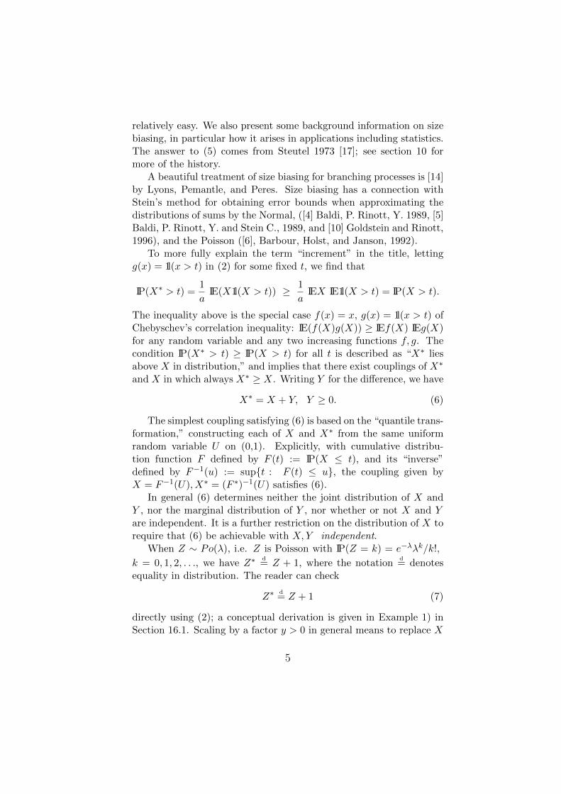
relatively easy. We also present some background information on sizebiasing, in particular how it arises in applications including statistics.The answer to (5) comes from Steutel 1973 [17]; see section 10 formore of the history.

A beautiful treatment of size biasing for branching processes is [14]by Lyons, Pemantle, and Peres. Size biasing has a connection withStein’s method for obtaining error bounds when approximating thedistributions of sums by the Normal, ([4] Baldi, P. Rinott, Y. 1989, [5]Baldi, P. Rinott, Y. and Stein C., 1989, and [10] Goldstein and Rinott,1996), and the Poisson ([6], Barbour, Holst, and Janson, 1992).

To more fully explain the term “increment” in the title, lettingg(x) = 1l(x > t) in (2) for some fixed t, we find that

IP(X∗ > t) =1

aIE(X1l(X > t)) ≥ 1

aIEX IE1l(X > t) = IP(X > t).

The inequality above is the special case f(x) = x, g(x) = 1l(x > t) ofChebyschev’s correlation inequality: IE(f(X)g(X)) ≥ IEf(X) IEg(X)for any random variable and any two increasing functions f, g. Thecondition IP(X∗ > t) ≥ IP(X > t) for all t is described as “X∗ liesabove X in distribution,” and implies that there exist couplings of X∗

and X in which always X∗ ≥ X. Writing Y for the difference, we have

X∗ = X + Y, Y ≥ 0. (6)

The simplest coupling satisfying (6) is based on the “quantile trans-formation,” constructing each of X and X∗ from the same uniformrandom variable U on (0,1). Explicitly, with cumulative distribu-tion function F defined by F (t) := IP(X ≤ t), and its “inverse”defined by F−1(u) := sup{t : F (t) ≤ u}, the coupling given byX = F−1(U), X∗ = (F ∗)−1(U) satisfies (6).

In general (6) determines neither the joint distribution of X andY , nor the marginal distribution of Y , nor whether or not X and Yare independent. It is a further restriction on the distribution of X torequire that (6) be achievable with X,Y independent.

When Z ∼ Po(λ), i.e. Z is Poisson with IP(Z = k) = e−λλk/k!,

k = 0, 1, 2, . . ., we have Z∗d= Z + 1, where the notation

d= denotes

equality in distribution. The reader can check

Z∗d= Z + 1 (7)

directly using (2); a conceptual derivation is given in Example 1) inSection 16.1. Scaling by a factor y > 0 in general means to replace X

5

by yX, and it follows easily from (2) that

(yX)∗ = y(X∗). (8)

For our case, multiplying (7) by y > 0 yields the implication, forPoisson Z,

if X = yZ, then X∗ = X + y. (9)

Hence, for each λ > 0 and y > 0, (9) gives an example where (5)is satisfied with Y a constant random variable, which is independentof every random variable. In a very concrete sense, all solutions of (5)can be built up from these examples, but to accomplish that we mustfirst review how to size bias sums of independent random variables.

4 How to size bias a sum of indepen-

dent random variables

Consider a sum X = X1 + · · · + Xn, with independent non-negativesummands Xi, and suppose that IEXi = ai, IEX = a. Write Si =X −Xi, so that Si and Xi are independent, and also take Si and X∗ito be independent; this is used to obtain the final inequality in (10)below.

We have for all bounded functions g,

IEg(X∗) = IE(Xg(X))/a

=n∑i=1

(ai/a)IE(Xig(Si +Xi))/ai

=

n∑i=1

(ai/a)IEg(Si +X∗i ). (10)

The result in (10) says precisely that X∗ can be represented by themixture of the distributions Si +X∗i with mixture probabilities ai/a.In words, in order to size bias the sum X with independent summands,we first pick an independent index I with probability proportional toits expectation, that is, with distribution IP(I = i) = ai/a, and thensize bias only the summand XI . Or, with X1, . . . , Xn, X

∗1 , . . . , X

∗n and

I all independent

(X1+X2+ · · ·+Xn)∗ = X1+ · · ·+XI−1+X∗I +XI+1+ · · ·+Xn. (11)

6

For the special case where the summands Xi are not only inde-pendent but also identically distributed, or i.i.d., this recipe simplifies.In this case it does not matter which summand is biased, as all thedistributions in the mixture are the same; hence for any i = 1, . . . , n,X∗

d= X1 + · · ·+Xi−1 +X∗i +Xi+1 + · · ·+Xn. In particular we may

use i = 1 so that

(X1 +X2 + · · ·+Xn)∗ = X∗1 +X2 +X3 + · · ·+Xn. (12)

5 Waiting for a bus: the renewal the-

ory connection

Renewal theory provides a conceptual explanation of the identity (12)and at the same time gives an explanation of the waiting time paradox.Let the interarrival times of our buses in Section 1 be denoted Xi,so that buses arrive at times X1, X1 + X2, X1 + X2 + X3, . . ., andassume only that the Xi are i.i.d., strictly positive random variableswith finite mean; the paradox presented earlier was the special casewith Xi exponentially distributed. Implicit in the story of my arrivaltime T as “arbitrary” is that my precise arrival time does not matter,and that there should be no relation between my arrival time and theschedule of buses. One way to model this assumption is to choose Tuniformly from 0 to l, independent of X1, X2, . . ., and then take thelimit as l → ∞; informally, just imagine some very large l. Such a Tcorresponds to throwing a dart at random from a great distance towardthe real line, which has been subdivided into intervals of lengths Xi.Naturally the dart is twice as likely to land in a given interval of lengthtwo than one of length one, and generally x times as likely to land ina given interval of length x as one of length one. In other words, ifthe interarrival times Xi have a distribution dF (x), the distributionof the length of the interval where the dart lands is proportional tox dF (x). The constant of proportionality must be 1/a, in order tomake a legitimate distribution, so the distribution of the interval wherethe dart lands is the distribution of X∗.

The conceptual explanation of identity (12) is the following. Sup-pose that every nth bus is bright blue, so that the waiting time be-tween bright blue buses is the sum over a block of n successive ar-rival times. Again, the random time T finds itself in an intervalwhose length is distributed as the size biased distribution of the in-

7

terarrival times; the length of the neighboring intervals are not af-fected. But by considering the variables as appearing in blocks ofn, the random time T must also find itself in a block distributed as(X1 + · · ·+Xn)∗. Since only the interval containing one of the interar-rival times has been size biased, this sum must be equal in distributionto X1 + · · ·+Xi−1 +X∗i +Xi+1 + · · ·+Xn.

A more precise explanation of our waiting time paradox is basedon the concept of stationarity — randomizing the schedule of buses sothat I can arrive at an arbitrary time t, and specifying a particular tdoes not influence how long I must wait for the next bus. The simpleprocess with arrivals at times X1, X1 + X2, X1 + X2 + X3, . . . is ingeneral not stationary; and the distribution of the time Wt that wewait from time t until the arrival of the next bus varies with t. Wecan, however, cook up a stationary process from this simple processby a modification suggested by size biasing. For motivation, recallthe case where I arrive at T chosen uniformly from (0, l). In thelimit as l → ∞ the interval containing T has length distributed asX∗i , and my arrival within this interval is ‘completely random.’ Thatis, I wait UX∗i for the next bus, and I missed the previous bus by(1−U)X∗i , where U is uniform on (0,1) and independent of X∗i . Thusit is plausible that one can form a stationary renewal process by thefollowing recipe. Extend X1, X2, . . . to an independent, identicallydistributed sequence . . . , X−2, X−1, X0, X1, X2, . . . . Let X∗0 be thesize biased version of X0 and let U be chosen uniformly in (0,1), withall variables independent. The origin is to occupy an interval of lengthX∗0 , and the location of the origin is to be uniformly distributed overthis interval; hence buses arrive at time UX∗0 and −(1−U)X∗0 . UsingX1, X2, . . . and X−1, X−2, . . . as interarrival times on the positive andnegative side, we obtain a process by setting bus arrivals at the positivetimes UX∗0 , UX

∗0 +X1, UX

∗0 +X1 +X2, · · · , and at the negative times

−(1−U)X∗0 ,−((1−U)X∗0 +X−1),−((1−U)X∗0 +X−1 +X−2), . . . ,and it can be proved that this process is stationary.

The interval which covers the origin has expected length IEX∗0 =IEX2

0/IEX0 (by (4) with n = 1,) and the ratio of this to IEX0 isIEX∗0/IEX0 = IEX2

0/(IEX0)2. By Cauchy-Schwarz, this ratio is at least

1; and every value in [1,∞] is feasible. Note that my waiting time isIEWT = IEW0 = IE(UX∗0 ) = (1/2)IEX∗0 , so the ratio of my waitingtime to the average time between buses can be any value between 1/2and infinity, depending on the distribution of the interarrival times.

The exponential case is very special, where strange and wonder-

8

ful “coincidences” effectively hide all the structure involved in sizebiasing and stationarity. The distribution of X∗0 , obtained by sizebiasing the unit exponential, has density xe−x for x > 0, using (3)with a = 1. This distribution is known as Gamma(1,2). In par-ticular, IEX∗i =

∫∞0 x(xe−x) dx = 2, and splitting this in half for

“symmetry” as in Feller’s answer (b) gives 1 as the expected time Imust wait for the next bus. Furthermore, the independent uniformU splits that Gamma(1,2) variable X∗0 into UX∗0 and (1 − U)X∗0 ,and these turn out to be independent, and each having the origi-nal exponential distribution. Thus the general recipe for cooking upa stationary process, involving X∗0 and U in general, simplifies be-yond recognition: the original simple schedule with arrivals at timesX1, X1+X2, X1+X2+X3, . . . forms half of a stationary process, whichis completed by its other half, arrivals at −X ′1,−(X ′1 +X ′2), . . . , withX1, X2, . . . , X

′1, X

′2, . . . all independent and exponentially distributed.

6 Size bias in statistics

But size biasing is not always undesired. In fact, it can be used toconstruct unbiased estimators of quantities that are at first glance dif-ficult to estimate without bias. Suppose we have a population of nindividuals, and associated to each individual i is the pair of real num-bers xi ≥ 0 and yi, with

∑xi > 0. Perhaps xi is how much the ith

customer was billed by their utility company last month, and yi, saya smaller value than xi, the amount they were supposed to have beenbilled. Suppose we would like to know just how severe the overbillingerror is; we would like to know the ’adjustment factor’, which is theratio

∑i yi/

∑i xi. Collecting the paired values for everyone is labo-

rious and expensive, so we would like to be able to use a sample ofm < n pairs to make an estimate. It is not too hard to verify thatif we choose a set R by selecting m pairs uniformly from the n, thenthe estimate

∑j∈R yj/

∑j∈R xj will be biased; that is, the estimate,

on average, will not equal the ratio we are trying to estimate.Here’s how size biasing can be used to construct an unbiased esti-

mate of the ratio∑

i yi/∑

i xi, using m < n pairs. Create a randomset R of size m by first selecting a pair with probability proportional toxi, and then m− 1 pairs uniformly from the remaining pairs. Thoughwe are out of the independent framework, the principle of (12) is stillat work; size biasing one has size biased the sum. (This is so because

9

we have size biased the one, and then chosen the others from an ap-propriate conditional distribution.) That is, one can now show thatby biasing to include the single element in proportion to its x value,we have achieved a distribution whereby the probability of choosingthe set r is proportional to

∑j∈r xj . From this observation it is not

hard to see why IE(∑

j∈R yj/∑

j∈R xj) =∑

i yi/∑

i xi. This methodis known as Midzuno’s procedure for unbiased ratio estimation, andis noted in Cochran [8].

7 Size biasing, tightness, and uniform

integrability

Recall that a collection of random variables {Yα : α ∈ I} is tight ifffor all ε > 0 there exists L <∞ such that

IP(Yα 6∈ [−L,L]) < ε for all α ∈ I.

This definition looks quite similar to the definition of uniform integra-bility, where we say {Xα : α ∈ I} is uniformly integrable, or UI, iff forall δ > 0 there exists L <∞ such that

IE(|Xα|;Xα /∈ [−L,L]) < δ for all α ∈ I.

Intuitively, tightness for a family is that uniformly over the family,the probability mass due to large values is arbitrarily small. Similarly,uniform integrability is the condition that, uniformly over the family,the contribution to the expectation due to large values is arbitrarilysmall.

Tightness of the family of random variables {Yα : α ∈ I} impliesthat every sequence of variables Yn, n = 1, 2, . . . from the family has asubsequence that converges in distribution. The concept of tightnessis very useful not just for random variables, that is, real-valued ran-dom objects, but also for random elements of other spaces; in moregeneral spaces, the closed intervals [−L,L] are replaced by compactsets. If {Xα : α ∈ I} is uniformly integrable, IEXn → IEX for anysequence of variables Xn, n = 1, 2, . . . from the family that convergesin distribution.

To discuss the connection between size biasing and uniform inte-grability, it is useful to restate the basic definitions in terms of non-negative random variables. It is clear from the definition of tightness

10

above that a family of nonnegative random variables {Yα : α ∈ I} istight iff for all ε > 0 there exists L <∞ such that

IP(Yα > L) < ε for all α ∈ I, (13)

and from the definition of UI, that a family of nonnegative randomvariables {Xα : α ∈ I} is uniformly integrable iff for all δ > 0 thereexists L <∞ such that

IE(Xα;Xα > L) < δ for all α ∈ I. (14)

For general random variables, the family {Gα : α ∈ I} is tight [respec-tively UI] iff {|Gα| : α ∈ I} is tight [respectively UI]. We specialize inthe remainder of this section to random variables that are non-negativewith finite, strictly positive mean.

Since size bias relates contribution to the expectation to probabil-ity mass, there should be a connection between tightness, size bias,and UI. However, care should be taken to distinguish between the (ad-ditive) contribution to expectation, and the relative contribution toexpectation. The following example makes this distinction clear. Let

IP(Xn = n) = 1/n2, IP(Xn = 0) = 1− 1/n2, n = 1, 2, . . . .

Here, IEXn = 1/n, the family {Xn} is uniformly integrable, but 1 =IP(X∗n = n), so the family {X∗n} is not tight. The trouble is that theadditive contribution to the expectation from large values of Xn issmall, but the relative contribution is large — one hundred percent!The following two theorems, which exclude this phenomenon, showthat tightness and uniform integrability are very closely related.

Theorem 7.1 Assume that for α ∈ I, where I is an arbitrary indexset, the random variables Xα satisfy Xα ≥ 0 and c ≤ IEXα < ∞, forsome c > 0. For each α let Yα = X∗α. Then

{Xα : α ∈ I} is UI iff {Yα : α ∈ I} is tight.

Proof. First, with Yα = X∗α, we have IP(Yα > L) = IE(1(Yα > L)) =IE(Xα1(Xα > L))/IEXα, so for any L and α ∈ I,

IE(Xα;Xα > L) = IEXαIP(Yα > L).

Assume that {Xα : α ∈ I} is UI, and let ε > 0 be given to testtightness in (13). Let L be such that (14) is satisfied with δ = εc.Now, using IEXα ≥ c, for every α ∈ I,

IP(Yα > L) = IE(Xα;Xα > L)/IEXα ≤ IE(Xα;Xα > L)/c < δ/c = ε,

11

establishing (13).Second, assume that {Xα : α ∈ I} if tight, and take L0 to satisfy

(13) with ε := 1/2, so that IP(Yα > L0) < 1/2 for all α ∈ I. Hence,for all α ∈ I,

IE(Xα;Xα > L0) = IEXαIP(Yα > L0) < IEXα/2,

and therefore,

L0 ≥ IE(Xα;Xα ≤ L0) = IEXα − IE(Xα;Xα > L0)

> IEXα − IEXα/2 = IEXα/2,

and hence IEXα < 2L0. Now given δ > 0 let L satisfy (13) for ε =δ/(2L0). Hence ∀α ∈ I,

IE(Xα;Xα > L) = IEXα IP(Yα > L) < 2L0 IP(Yα > L) < 2L0 ε = δ,

establishing (14).

Theorem 7.2 Assume the for α ∈ I, where I is an arbitrary indexset, that random variables Xα satisfy Xα ≥ 0 and IEXα < ∞. Pickany c ∈ (0,∞), and for each α let Yα = (c+Xα)∗. Then

{Xα : α ∈ I} is UI iff {Yα : α ∈ I} is tight.

Proof. By Theorem 7.1, the family {c + Xα} is UI iff the family{(c + Xα)∗} is tight. As it is easy to verify that the family {Xα} istight [respectively UI] iff the family {c+Xα} is tight [respectively UI],Theorem 7.2 follows directly from Theorem 7.1.

8 Size biasing and infinite divisibility:

the heuristic

Because of the recipe (12), it is natural that our question in (5) isrelated to the concept of infinite divisibility. We say that a randomvariable X is infinitely divisible if for all n, X can be decomposed indistribution as the sum of n iid variables. That is, that for all n there

exists a distribution dFn such that if X(n)1 , . . . , X

(n)n are iid with this

distribution, then

Xd= X

(n)1 + · · ·+X(n)

n . (15)

12

Because this is an iid sum, by (12), we have

X∗ = (X −X(n)1 ) + (X

(n)1 )∗,

with X −X(n)1 and (X

(n)1 )∗ independent. For large n, X −X(n)

1 willbe close to X, and so we have represented the size bias distribution ofX as approximately equal, in distribution, to X plus an independentincrement. Hence it is natural to suspect that the class of non negativeinfinitely divisible random variables can be size biased by adding anindependent increment.

It is not difficult to make the above argument rigorous, for infinitely

divisible X ≥ 0 with IEX <∞. First, to show that X−X(n)1 converges

in distribution to X, it suffices to show that X(n)1 converges to zero

in probability. Note that X ≥ 0 implies X(n)1 ≥ 0, since (15) gives

0 = IP(X < 0) ≥ (IP(X(n)1 < 0)n. Then, given ε > 0, ∞ > IEX ≥

nIP(X(n)1 > ε)ε implies that IP(X

(n)1 > ε) → 0; hence X

(n)1 → 0 in

probability as n→∞.We have that

X∗ = (X −X(n)1 ) + (X

(n)1 )∗, (16)

with X − X(n)1 and (X

(n)1 )∗ independent, and X − X(n)

1 converging

to X in distribution. Now, the family of random variables (X(n)1 )∗ is

“tight”, because given ε > 0, there is a K such that IP(X∗ > K) < ε,

and by (16), for all n, IP((X(n)1 )∗ > K) ≤ IP(X∗ > K) < ε. Thus,

by Helly’s theorem, there exists a subsequence nk of the n’s along

which (X(n)1 )∗ converges in distribution, say (X

(nk)1 )∗

distr−→ Y . Takingn → ∞ along this subsequence, the pair (X − Xn

1 , (Xn1 )∗) converges

jointly to the pair (X,Y ) with X and Y independent. From X∗ =

(X − X(nk)1 ) + (X

(nk)1 )∗

distr−→ X + Y as k → ∞ we conclude that

X∗d= X + Y , with Y ≥ 0, and X,Y independent. This concludes a

proof that if X ≥ 0 with 0 < IEX < ∞ is infinitely divisible, then itsatisfies (5).

9 Size biasing and Compound Poisson

Let us now return to our main theme, determining for which distri-butions we have (5). We have already seen it is true, trivially, for a

13

scale multiple of a Poisson random variable. We combine this withthe observation (11) that to size bias a sum of independent randomvariables, just bias a single summand, chosen proportional to its ex-pectation. Consider a random variable of the form

X =n∑1

Xj , with Xj = yjZj , Zj ∼ Po(λj), Z1, . . . , Zn independent,

(17)with distinct constants yj > 0.

Since X is a sum of independent variables, we can size bias X bythe recipe (11); pick a summand proportional to its expectation andsize bias that one. We have EXj = yjλj and therefore a = EX =∑

j yjλj . Hence, the probability that we pick summand j to size biasis

IP(I = j) = yjλj/a.

But by (9), X∗j = Xj + yj , so that when we pick Xj to bias we addyj . Hence, to bias X we merely add yj with probability yjλj/a, or, toput it another way X∗ = X + Y , with X,Y independent and

IP(Y = yj) = yjλj/a. (18)

In summary, X of the form (17) can be size biased by adding anindependent, nonnegative increment. It will turn out that we havenow nearly found all solutions of (5), which will be obtained by takinglimits of variables type (17) and adding a nonnegative constant.

Sums of the form (17) are said to have a compound Poisson distri-bution — of finite type. Compound Poisson variables in general areobtained by a method which at first glance looks unrelated to (17),considering the sum SN formed by adding a Poisson number N of iidsummands A1, A2, . . . from any distribution, i.e. taking

Xd= SN := A1 + · · ·+AN , N ∼ Po(λ), (19)

where N,A1, A2, . . . are independent and A1, A2, . . . identically dis-tributed. The notation SN := A1 + . . .+AN reflects that of a randomwalk, Sn := A1 + · · ·An for n = 0, 1, 2, . . ., with S0 = 0.

To fit the sum (17) into the form (19), let λ =∑λj and let

A,A1, A2, . . . be iid with

IP(A = yj) = λj/λ. (20)

14

The claim is that X as specified by (17) has the same distributionas the sum SN . Checking this claim is most easily done with gen-erating functions, such as characteristic functions, discussed in thenext section. Nevertheless, it is an enjoyable exercise for the specialcase where a1, . . . , an are mutually irrational, i.e. linearly independentover the rationals, so that with k1, . . . , kn integers, the sum

∑n1 kjaj

determines the values of the kj .Note that the distribution (20) of the summands Ai is different

from the distribution in (18). In fact, A∗d= Y , which can be checked

using (20) together with (3), and comparing the result to (18):

IP(A∗ = yj) =yjIP(A = yj)

IEA=

yjλj/λ∑k ykλk/λ

=yjλj∑k ykλk

= IP(Y = yj).

(21)Thus the result that for the compound Poisson of finite type, X∗ =X + Y can be expressed as

(SN )∗ = SN + Yd= A1 + · · ·+AN +A∗, (22)

with all summands independent. Note how this contrasts with therecipe (12) for size biasing a sum with a deterministic number of termsn; in the case of (12) the biased sum and the original sum have thesame number of terms, but in (22) the biased sum has one more termthan the original sum.

If we want to size bias a general compound Poisson random variableSN , there must be some restrictions on the distribution for the iidsummands Ai in (19). First, since λ > 0, and (using the independenceof N and S0, S1, . . .,) IESN = IEN IEA = λIEA, the condition thatIESN ∈ (0,∞) is equivalent to IEA ∈ (0,∞). The condition thatSN ≥ 0 is equivalent to the condition Ai ≥ 0. We choose the additionalrequirement that A be strictly positive, which is convenient since itenables the simple computation IP(SN = 0) = IP(N = 0) = e−λ.There is no loss of generality in this added restriction, for if p :=IP(A = 0) > 0, then with M being Poisson with parameter IEM =λ(1− p), and B1, B2, . . . iid and independent of M , with IP(B ∈ I) =IP(A ∈ I)/(1− p) for I ⊂ (0,∞) (using p < 1 since IEA > 0), we have

A1 + · · ·+ ANd= B1 + · · ·+ BM , so that SN can be represented as a

compound Poisson with strictly positive summands.

15

10 Compound Poisson vs. Infinitely

Divisible

We now have two ways to produce solutions of (5), infinitely divisibledistributions from section 8, and finite type compound Poisson distri-butions, from (17), so naturally the next question is: how are theserelated?

The finite type compound Poisson random variable in (17) can beextended by adding in a nonnegative constant c, to get X of the form

X = c+

n∑1

Xj , with Xj = yjZj , Zj ∼ Po(λj), Z1, . . . , Zn independent,

(23)with c ≥ 0 and distinct constants yj > 0. In case c > 0, this randomvariable is not called compound Poisson. Every random variable of

the form (23) is infinitely divisible – for the X(m)i [for i = 1 to m in

(15)] simply take a sum of the same form, but with c replaced by c/mand λj replaced by λj/m.

The following two facts are not meant to be obvious. By tak-ing distributional limits of sums of the form (23), and requiring thatc+∑n

1 yjλj stays bounded as n→∞, one gets all the non-negative in-finitely divisible distributions with finite mean. By also requiring thatc = 0 and

∑n1 λj stays bounded, the limits are all the finite mean,

non-negative compound Poisson distributions.To proceed, we calculate the characteristic function for the distri-

bution in (17). First, if X is Po(λ), then

φX(u) := IEeiuX =∑k≥0

eiukIP(X = k) =∑

eiuke−λλk

k!= e−λ

∑ (λeiu)k

k!= exp(λ(eiu−1)).

For a scalar multiple yX of a Poisson random variable,

φyX(u) = IEeiu(yX) = IEei(yu)X = φX(yu) = exp(λ(eiuy − 1)).

Thus the summand Xj = yjZj in (17) has characteristic functionexp(λj(e

iuyj − 1)), and hence the sum X has characteristic function

φX(u) =n∏j=1

exp(λj(e

iuyj − 1))

= exp

n∑j=1

λj(eiuyj − 1)

.

16

To prepare for taking limits, we write this as

φX(u) = exp

(n∑1

λj(eiuyj − 1)

)= exp

( ∫(0,∞)

(eiuy − 1) µ(dy)

),

(24)where µ is the measure on (0,∞) which places mass λj at location yj .The total mass of µ is

∫1 µ(dy) =

∑n1 λj , which we will denote by λ,

and the first moment of µ is∫y µ(dy) =

∑n1 yjλj , which happens to

equal a := IEX.Allowing the addition of a constant c, the random variable of the

form (23) has characteristic function φX whose logarithm has the formlog φX(u) = iuc+

∫(0,∞)(e

iuy − 1) µ(dy), where µ is a measure whosesupport consists of a finite number of points. The finite mean, notidentically zero distributional limits of such random variables yield allof the finite mean, nonnegative, not identically zero, infinitely divisi-ble distributions. A random variable X with such a distribution hascharacteristic function φX with

log φX(u) = iuc+

∫(0,∞)

(eiuy − 1) µ(dy), (25)

where c ≥ 0, µ is any nonnegative measure on (0,∞) such that∫y µ(dy) <∞, and not both c and µ are zero.

Which of the distributions above are compound Poisson? Thecompound Poisson variables are the ones in which c = 0 and λ :=µ((0,∞)) <∞. With this choice of λ for the parameter of N , we have

Xd= SN as in (19), with the distribution of A given by µ/λ, i.e. IP(A ∈

dy) = µ(dy)/λ. To check, note that for X = SN , φX(u) := IEeiuSN =∑n≥0 IP(N = n)eiuSn = e−λ

∑n≥0 λ

n/n!(φA(u))n = exp(λ(φA(u)−1)

= exp(λ(∫(0,∞)(e

iuy − 1) IP(A ∈ dy), which is exactly (25) with c = 0.In our context, it is easy to tell whether or not a given infinitely

divisible random variable is also compound Poisson — it is if and onlyif IP(X = 0) is strictly positive — corresponding to IP(N = 0) = e−λ

and e−∞ = 0. Among the examples of infinitely divisible randomvariables in section 16.2, the only compound Poisson examples are theGeometric and Negative binomial family, and the distributions relatedto Buchstab’s function.

In (18) — specifying the distribution of the increment Y whenX∗ = X + Y with X,Y independent — the factor yj on the righthand side suggests another way to write (25). We multiply and divide

17

by y to get

log φX(u) =

∫[0,∞)

eiuy − 1

yν(dy), (26)

where ν is any nonnegative measure on [0,∞) with total mass ν( [0,∞) ) ∈(0,∞). The measure ν on [0,∞) is related to c and µ by ν({0}) = cand for y > 0, ν(dy) = y µ(dy); we follow the natural conventionthat (eiuy − 1)/y for y = 0 is interpreted as iu. The measure ν/a is aprobability measure on [0,∞) because

a := IEX = −i(d log φX(u)/du)|u=0 = c+

∫(0,∞)

y µ(dy) = c+ν((0,∞)) = ν([0,∞)).

(27)We believe it is proper to refer to either (25) or (26) as a Levy rep-resentation, and to refer to either µ or ν as the Levy measure, inhonor of Paul Levy; indeed when restriction that X be nonnegativeis dropped, there are still more forms for the Levy representation, seee.g. [9] Feller volume II, chapter XVII.

It is not hard to see that any distribution specified by (26) satisfies(5), by the following calculation with characteristic functions. Notethat for g(x) := eiux, the characterization (2) of the distribution of X∗

directly gives the characteristic function φ∗ of X∗ as φ∗(u) := IEeiuX∗

= IE(XeiuX)/a. For any X ≥ 0 with finite mean, by an application ofthe dominated convergence theorem, if φ(u) := IEeiuX then φ′(u) =IE(iXeiuX). Thus for any X ≥ 0 with 0 < a = IEX <∞,

φ∗(u) =1

iaφ′(u). (28)

Now if X has characteristic function φ given by (26), again usingdominated convergence,

φ′(u) = φ(u)

(ic+

∫(0,∞)

iyeiuy µ(dy)

)= ia φ(u)

∫[0,∞)

eiuyν(dy)/a.

(29)Taking the probability measure ν/a as the distribution of Y , andwriting η for the characteristic function of Y , (29) says that φ′(u) =ia φ(u) η(u). Combined with (28), we have

φ∗ = φ η. (30)

Thus X∗ = X + Y , with X and Y independent and L(Y ) = ν/a.

18

For the compound Poisson case in general, in which the distribu-tion of A is µ/λ, we have Y

d= A∗ because a := IEX = λ IEA and

IP(A∗ ∈ dy) = yIP(A ∈ dy)/IEA =y(µ(dy)/λ)

a/λ= ν(dy)/a = IP(Y ∈ dy),

(31)which can be compared discrete version (20). Thus the computation(30) shows, for the compound Poisson case, that (22) holds.

11 Main Result

Our main result is essentially the converse of the computation (30).

Theorem 11.1 (Steutel 1973 [17] ) For a random variable X ≥ 0with a := IEX ∈ (0,∞), the following three statements are equivalent.

i) There exists a coupling with X∗ = X + Y, Y ≥ 0, and X,Yindependent.

ii) The distribution of X is infinitely divisible,iii) The characteristic function of X has the Levy representation

(26).Furthermore, when any of these statements hold, the Levy measure

ν in (26) equals a times the distribution of Y .

Proof. We have proved that ii) implies i), in section 8. We haveproved that iii) implies i), in the argument ending with (30), whichalso shows that given ν in the Levy representation (26), the incrementY in i) has distribution ν/a.

The equivalence of ii) and iii) is a standard textbook topic — withthe argument for iii) implies ii) being simply that X with a given ν isthe sum of n iid terms each having the Levy representation (26) withν/n playing the role of ν.

Now to prove that i) implies ii), we assume that i) holds. Thecharacteristic function φ∗ of X∗ has the form φ∗ = φ η, where φ and ηare the characteristic functions of X and Y , so that η(u) = IEeiuY =∫[0,∞) e

iuy IP(Y ∈ dy). Combining this with (28) we have

1

iaφ′(u) = φ∗(u) = φ(u) η(u)

19

so that (log φ(u))′ = ia η(u). Since log φ(0) = 0,

log φ(u) = ia

∫s∈[0,u)

η(s) ds

= ia

∫s∈[0,u)

∫y∈[0,∞)

eisy IP(Y ∈ dy) ds

= ia

∫y∈[0,∞)

∫s∈[0,u)

eisy ds IP(Y ∈ dy)

= ia

(∫y∈(0,∞)

∫s∈[0,u)

eisy ds IP(Y ∈ dy) + uIP(Y = 0)

)

= a

∫y∈[0,∞)

eiuy − 1

yIP(Y ∈ dy).

This is the same as the representation (26), with ν = aL(Y ) for therandom variable Y given in i).

Observe that ν is an arbitrary probability distribution on [0,∞),i.e. ν ∈Pr([0,∞)), and the choice of a ∈ (0,∞) is also arbitrary. Thusthere is a one-to-one correspondence between the Cartesian productPr([0,∞))× (0,∞) and the set of the nonnegative, infinitely divisibledistributions with finite, strictly positive mean.

12 A consequence of X∗ = X + Y with

independence

To paraphrase the result of Theorem 11.1, for a nonnegative randomvariable X with a := IEX ∈ (0,∞), it is possible to find a couplingwith X∗ = X + Y , Y ≥ 0 and X,Y independent if and only if thedistribution of X is the infinitely divisible distribution with Levy rep-resentation (26) governed by the finite measure ν equal to a timesthe distribution of Y . Thus we know an explicit, albeit complicated,relation between the distributions of X and Y . It is worth seeing how(5) directly gives a simple relation between the densities of X and Y ,if these densities exist.

In the discrete case, if X has a mass function fX and if (26) holds,then Y must mass function, fY , and by (5), fX∗ is the convolution offX and fY : fX∗(x) =

∑y fX(x − y)fY (y). Combined with (3), this

20

says that for all x > 0,

fX(x) =a

x

∑y

fX(x− y)fY (y).

Likewise, in the continuous case, if X has density fX (i.e. if for allbounded g, IEg(X) =

∫g(x)fX(x) dx,) and if (26) holds, and if further

Y has a density fY , then by (5), fX∗ is the convolution of fX and fY :fX∗(x) =

∫y fX(x− y)fY (y). Combined with (3), this says that for all

x > 0,

fX(x) =a

x

∫yfX(x− y)fY (y) dy. (32)

13 Historical remark

For all intents and purposes, Theorem 11.1 is due to Steutel [17]. Theway he states his result is sufficiently different from our Theorem 11.1that for comparison, we quote verbatim from [17], p. 136:Theorem 5.3. A d.f. F on [0,∞) is infinitely divisible iff it satisfies

(5.6)

∫ x

0u dF (u) =

∫ x

0F (x− u) dK(u),

where K is non-decreasing.Observe that Steutel’s result is actually more general than Theo-

rem 11.1, since that latter only deals with nonnegative infinitely di-visible random variables with finite mean. The explicit connectionbetween the independent increment for size biasing, and the Levy rep-resentation, is made in [11], along with further connections betweenrenewal theory and independent increments.

14 The product rule for size biasing

We have seen that for independent, nonnegative random variablesX1, . . . , Xn, the sum X = X1 +X2 · · ·+Xn can be size biased by pick-ing a single summand at random with probability proportional to itsexpectation, and replacing it with one from its size biased distribution.Is there a comparable procedure for the product W = X1X2 · · ·Xn?Would it involve size-biasing a single factor?

21

Let ai = IEXi ∈ (0,∞), let Fi be the distribution function ofXi, and let F ∗i be the distribution function of X∗i , so that dF ∗i (x) =x dFi(x)/ai. Let X∗1 , . . . , X

∗n be independent. By (2) with a := IEW =

a1a2 · · · an, for all bounded functions g,

Eg(W ∗) = E (Wg(W )) /(a1a2 · · · an)

=

∫· · ·∫x1 · · ·xn g(x1x2 · · ·xn) dF1(x1) · · · dFn(xn)/(a1 · · · an)

=

∫· · ·∫g(x1x2 · · ·xn) (x1 dF1(x1)/a1) · · · (xn dFn(xn)/an)

=

∫· · ·∫g(x1x2 · · ·xn) dF ∗1 (x1) · · · dF ∗n(xn)

= Eg(X∗1 · · ·X∗n),

and soW ∗

d= X∗1 · · ·X∗n.

We have shown that to size bias a product of independent variables,one must size bias every factor making up the product, very muchunlike what happens for a sum, where only one term is size biased!

15 Size biasing the lognormal distri-

bution

The lognormal distribution is often used in financial mathematics tomodel prices, salaries, or values. A variable L with the lognormaldistribution is obtained by exponentiating a normal variable. We fol-low the convention that Z denotes a standard normal, with IEZ = 0,var Z = 1, so that L = eZ represents a standard lognormal. Withconstants σ > 0, µ ∈ IR, σZ + µ represents the general normal, andL = eσZ+µ represents the general lognormal. As the lognormal isnon-negative and has finite mean, it can be size biased to form L∗.

One way to guess the identity of L∗ is to use the method of mo-ments. For the standard case L = eZ , for any real t, calculation givesIEetZ = exp(t2/2). Taking t = 1 shows that IEL =

√e, and more

generally, for n = 1, 2, . . ., IELn = IEenZ = exp(n2/2). Using relation(4), the moment-shift for size biasing, we have IE(L∗)n = IELn+1/IEL= exp((n+1)2/2−1/2) = exp(n2/2+n) = enIELn = IE(eL)n. Clearly

we should guess that L∗d= eL, but we must be cautions, as the most

famous example of a distribution which has moments of all orders

22

but which is not determined by them is the lognormal; for other suchdistributions related to the normal, see [16].

We present a rigorous method for finding the distribution of L∗,based on the size biasing product rule of the previous section; as anexercise the reader might try to verify our conclusion (33) by workingout the densities for lognormal distributions, and using the relation(3).

We begin with the case µ = 0, σ > 0. Let Ci be independentvariables taking the values 1 or −1 with equal probability. Thesevariables have mean zero and variance one, and by the central limittheorem, we know that

1√n

n∑i=1

σCidistr−→ σZ.

Hence, we must have

W =

n∏i=1

exp(1√nσCi) = exp(

1√n

n∑i=1

σCi)distr−→ exp(σZ) = L,

a lognormal, and thus W ∗distr−→ L∗. Write Xi := exp(σCi/

√n), so

that W = X1 · · ·Xn with independent factors, and by the productrule, W ∗ = X∗1 · · ·X∗n. The variables Xi take on the values q = e−σ/

√n

and p = eσ/√n with equal probability, and so X∗i take on these same

values, but with probabilities q/(p + q) and p/(p + q) respectively.Let’s say that Bn of the X∗i take the value p, so that n − Bn of theX∗i take the value q. Using Bn, we can write

W ∗ = pBnqn−Bn = eσ(2Bn−n)/√n.

Since Bn counts the number of “successes” in n independent trials,with success probability p/(p+q), Bn is distributed binomial(n, p/(p+q)). As n → ∞, the central limit theorem gives that Bn has an ap-proximate normal distribution. Doing a second order Taylor expan-sion of ex around zero, and applying it at x = ±σ/

√n, we find that

p/(p + q) = 1/2 + σ/(2√n) + O(1/n), so that Bn is approximately

normal, with mean np/(p+ q) = (1/2)(n+ σ√n) +O(1) and variance

npq/(p+ q)2 = n/4 +O(1/n3/2). Hence

1√n

(2Bn − n)distr−→ Z + σ as n→∞

23

and therefore

W ∗distr−→ eσ(Z+σ).

Since W ∗distr−→ L∗ = (eσZ)∗, we have shown that (eσZ)∗

d= eσ(Z+σ).

For the case where L = eσZ+µ, the scaling relation (8) yields theformula for size biasing the lognormal in general:

(eσZ+µ)∗ = eσ(Z+σ)+µ. (33)

16 Examples

In light of Theorem 11.1, for a nonnegative random variable X withfinite, strictly positive mean, being able to satisfy X∗ = X + Y withindependence and Y ≥ 0 is equivalent to being infinitely divisible. Wegive examples of size biasing, first with examples that are not infinitelydivisible, then with examples that are.

16.1 Examples of size biasing without an in-dependent increment

Both examples 1 and 2 below involve bounded, nonnegative randomvariables. Observe that in general, the distributions of X and X∗

have the same support, except that always IP(X∗ = 0) = 0. Thisimmediately implies that if X is bounded but not constant, then itcannot satisfy (5).

Example 1. Bernoulli and binomialLet Bi be Bernoulli with parameter p ∈ (0, 1], i.e. Bi takes the

value 1 with probability p, and the value 0 with probability 1 − p.Clearly B∗i = 1, since IP(B∗1 = 1) = 1IP(B1 = 1)/IEB1 = 1. IfB1, B2, . . . are independent, and Sn = B1 + · · ·+Bn we say that Sn ∼binomial (n, p). We size bias Sn by size biasing a single summand,

so S∗nd= Sn−1 + 1, which cannot be expressed as Sn + Y with Sn, Y

independent!Note that letting n→∞ and np→ λ in the relation S∗n

d= Sn−1+1

gives another proof that X∗d= X + 1 when X ∼ Po(λ), because both

Sn−1distr−→ X and Sn

distr−→ X. Here we have a family of exampleswithout independence, whose limit is the basic example with indepen-dence.

24

Example 2. Uniform and BetaThe Beta distribution on (0,1), with parameters a, b > 0 is specified

by saying that its has a density on (0,1), proportional to (1−x)a−1xb−1.The uniform distribution on (0,1) is the special case a = b = 1 of thisBeta family. Using (3), if X ∼ Beta(a, b), then X∗ ∼ Beta(a, b+ 1).

There are many families of distributions for which size biasingsimply changes the parameters; our examples are the Beta family inexample 2, the negative binomial family in example 4, the Gammafamily in example 5, and the lognormal family in example 6. In thesefamilies, either all members satisfy (5), or else none do. Thus it mightbe tempting to guess that infinite divisibility is a property preservedby size biasing, but it ain’t so.Example 3. X = 1 +W where W is Poisson

We have X∗ is a mixture of X + 0 and X + 1, using (11) withX1 = 1, X∗1 = X1 + 0 and X2 = W , X∗2 = W + 1. That is, X∗ isa mixture of 1 + W , with weight 1/(1 + λ), and 2 + W , with weightλ/(1+λ). Elementary calculation shows that it is not possible to haveX∗ = X + Y with X,Y independent and Y ≥ 0. Therefore X is notinfinitely divisible.

Since X = W ∗, we have an example in which W is infinitely divis-ible, but W ∗ is not.

16.2 Examples of X∗ = X + Y with indepen-dence

By Theorem 11.1, when X satisfies X∗d= X + Y with X,Y indepen-

dent and Y ≥ 0, the distribution of X is determined by the distribu-tion of Y together with a choice for the constant a ∈ (0,∞) to serve asIEX. Thus all our examples below, organized by a choice of Y , comein one parameter families indexed by a — or if more convenient, bysomething proportional to a; in these families, X varies and Y staysconstant!

Example 4. Y is 1+geometric. X is geometric or negativebinomial

4a) The natural starting point is that you are given the geomet-ric distribution: IP(X = j) = (1 − q)qj for j ≥ 0, with 0 < q <1, and you want to discover whether or not it is infinitely divisi-ble. Calculating the characteristic function, φ(u) =

∑k≥0 e

iuk(1 −

25

q)qk = (1 − q)/(1 − qeiu), so log φ(u) = log(1 − q) − log(1 − qeiu)= −

∑j≥1 q

j/j +∑

j≥1(qjeiuj/j) =

∑j≥1((e

iuj − 1)/j) qj .Thus the geometric distribution has a Levy representation in which

ν has mass qj at j = 1, 2, . . ., so we have verified that the geometricdistribution is infinitely divisible. The total mass a of ν is a = q +q2 + · · · = q/(1 − q); and this agrees with the recipe a = IEX. Since

IP(Y = j) = ν({j})/a = (1 − q)qj−1 for j = 1, 2, . . ., we have Yd=

1 +X. Thus X∗ = X + Y with X,Y independent and Yd= X + 1.

4b) Multiplying the Levy measure ν by t > 0 yields the general caseof the negative binomial distribution, X ∼ negative binomial(t, q).The case t = 1 is the geometric distribution. We still have X∗ = X+Ywith X,Y independent, and Y ∼ geometric(q) + 1. Note that forinteger t we can verify our calculation in another way, as in this caseX is the sum of t independent geometric(q) variables Xi. By (12),we can size bias X by size biasing a single geometric term, which isthe same as adding an independent Y with distribution, again, 1 +geometric(q).

Example 5. Y is exponential. X is exponential or Gamma5a) Let X be exponentially distributed with IEX = 1/α, i.e.

IP(X > t) = e−αt for t > 0. As we saw in section 5 for the case

α = 1, X∗ = X + Y with X,Y independent and Yd= X. The case

with general α > 0 is simply a spatial scaling of the mean one, “stan-dard” case. The Levy measures ν is simply IEX = 1/α times thecommon distribution of X and Y , with ν(dy) = e−αy dy

5b) Multiplying the Levy measure ν by t > 0 yields the general caseof the Gamma distribution, X ∼ Gamma(α, t). The name comes fromthat fact thatX has density f(x) = (αt/Γ(t)) xt−1e−αx on (0,∞). Thespecial case t = 1 is the exponential distribution, and more generallythe case t = n can be realized as X = X1 + · · ·+Xn where the Xi areiid, exponentially distributed with IEXi = 1/α. We have X∗ = X+Ywith X,Y independent and Y is exponentially distributed with mean(1/α), so thatX∗ ∼Gamma(α, t+1). The Levy measure here is ν withν(dy) = te−αy dy; so the corresponding µ has µ(dy) = te−αy/y dy.This form of µ is known as the Moran or Gamma subordinator; seee.g. [13]. As in example 4b), for integer t we can verify our calculationby noting that X is the sum of t independent exponential, mean (1/α)variables, and that by (12), when size biasing we will get the same Yadded on to the sum as the Y which appears when size biasing anysummand.

26

Example 6. Y is ??, X is lognormalAs mentioned in Section (15), we say that X is lognormal when

X = eσZ+µ where Z is a standard normal variable. The proof thatthe lognormal is infinitely divisible, first given by Thorin [19], remainsdifficult; there is an excellent book by Bondesson [7] for further study.Consider even the standard case, X = eZ , so that by equation (15),

X∗d= eZ+1 d

= eX. The result of Thorin that this X is infinitely di-visible is thus equivalent, by Theorem 11.1, to the claim that thereexists a distribution for Y ≥ 0 such that with X and Y independent,X + Y

d= eX. Also, by Theorem 11.1 with a = IEX =

√e, the distri-

bution of Y is exactly 1/√e times the Levy measure ν. However, there

does not seem to exist yet a simplified expression for this distribution!Since the lognormal X = eZ satisfies X∗ = eX = X + (1− e)X, it

provides a simple illustration of our remarks in the paragraph following(6), that the relation X∗ = X + Y, Y ≥ 0 does not determine thedistribution of Y without the further stipulation that X and Y beindependent. Note also that in X∗ = X + (1 − e)X, the increment(1 − e)X is a monotone function of X, so this is an example of thecoupling using the quantile transformation.

Example 7. Y is uniform on an interval (β, γ), with 0 ≤ β <γ <∞. By scaling space (dividing by γ) we can assume without lossof generality that γ = 1. This still allows two qualitatively distinctcases, depending on whether β = 0 or β > 0.

Example 7a. β = 0: Dickman’s function and its convolutionpowers.

With a = IEX ∈ (0,∞), this example is specified by (26) with νbeing a times the uniform distribution on (0,1), so that µ(dx) = a/x dxon (0, 1). The reader must take on faith that ν having a density,together with µ( (0,∞) ) =∞ so that IP(X = 0) = 0, implies that thedistribution of X has a density, call it ga. Size biasing then gives aninteresting differential-difference equation for this density: using (32),for x > 0,

ga(x) =a

x

∫ 1

y=0ga(x− y) dy =

a

x

∫ x

x−1ga(z) dz. (34)

Multiplying out gives xga(x) = a∫ xx−1 ga(z) dz, and taking the deriva-

tive with respect to x yields xg′a(x) + ga(x) = aga(x)− aga(x− 1), sothat g′a(x) = ( (a− 1)ga(x)− aga(x− 1) )/x, for x > 0.

27

For the case a = 1 this simplifies to g′1(x) = −g1(x−1)/x, which isthe same differential-difference equation that is used to specify Dick-man’s function ρ, of central importance in number theory; see [18].The function ρ is characterized by ρ(x) = 1 for 0 ≤ x ≤ 1 and ρ′(x) =−ρ(x − 1)/x for x > 0, and ρ(x) = 0 for x < 0, with ρ continuouson [0,∞), and from the calculation that

∫∞0 ρ(x) dx = eγ , where γ is

Euler’s constant, it follows that g1(x) = e−γρ(x). Dickman’s functiongoverns the distribution of the largest prime factor of a random integerin the following sense: for fixed u > 0, the proportion of integers from1 to n whose largest prime factor is smaller than n1/u tends to ρ(u)as n → ∞. For example, ρ(2) can be calculated from the differentialequation simply by ρ(2) = ρ(1) +

∫ 21 ρ′(x) dx = 1 +

∫ 21 −ρ(x− 1)/x dx

= 1 +∫ 21 −1/x dx = 1 − log 2

.= 1 − .69314 = .30686, and the claim

is that ρ(2) gives, for large n, the approximate proportion of integersfrom 1 to n all of whose prime factors are at most

√n.

For general t > 0 the density gt is a “convolution power of Dick-man’s function,” see [12]. The size bias treatment of this first appearedin the 1996 version of [2], and was subsequently written up in [1].

Example 7b. β > 0: Buchstab’s function, integers free ofsmall prime factors.

For these examples Y is uniform on (β, 1) for β ∈ (0, 1), withdensity 1/(1 − β) on (β, 1). Therefore ν is a multiple of uniformdistribution on (β, 1), with density t on (β, 1) for some constant t > 0— we have a := IEX = t(1−β) — but t rather than a is the convenientparameter. From ν(dx) = t dx on (β, 1) we get µ(dx) = t/x dx on(β, 1), so that the total mass of µ is λ =

∫(β,1) t/x dx = t log(1/β).

Since λ <∞, X is compound Poisson with IP(X = 0) = e−λ = βt.For the case t = 1, the distribution of the random variable X is

related to another important function in number theory, Buchstab’sfunction ω; again see [18]. The relation involves a “defective density”— here t = 1 and IP(X = 0) = β > 0 so X does not have a properdensity. Size biasing yields a relation similar to (32), which leads to adifferential-difference equation, which in turn establishes the relationbetween the defective density and Buchstab’s function; see [3]. The

net result is that for β < a < b < 1, IP(a < X < b) =∫ ba ω(x/β) dx.

Buchstab’s function ω is characterized by the properties that it iscontinuous on (1,∞), ω(u) = 1/u for u ∈ [1, 2], and (uω(u))′ = ω(u−1) for u > 2. It governs the distribution of the smallest prime factorof a random integer in the sense that for u > 1, the proportion of

28

integers form 1 to n whose smallest prime factor is at least n1/u isasymptotic to uω(u)/ log n.

References

[1] Arratia, R. (1998) On the central role of the scale invariant Pois-son processes on (0,∞). In D. Aldous and J. Propp editors, Mi-crosurveys in Discrete Probability, pages 21-41, DIMACS Seriesin Discrete Math. and Theoret. Comput. Sci., Amer. Math. Soc.,Providence RI.

[2] Arratia, R., Barbour, A. D., and Tavare, S. (1997) Logarithmiccombinatorial structures. Monograph, 187 pages, in preparation.

[3] Arratia, R., and Stark, D. (1998) A total variation distance invari-ance principle for primes, permutations and Poisson-Dirichlet.Preprint.

[4] Baldi, P. Rinott, Y. (1989). On normal approximations of distri-butions in terms of dependency graphs, Annals of Probability 17, 1646-1650.

[5] Baldi, P. Rinott, Y. and Stein, C. (1989). A normal approxima-tions for the number of local maxima of a random function ona graph. In Probability, Statistics and Mathematics, Papers inHonor of Samuel Karlin. T. W. Anderson, K.B. Athreya and D.L. Iglehart eds., Academic Press , 59-81.

[6] Barbour, Holst, and Janson (1992). Poisson Approximation. Ox-ford Science Publications.

[7] Bondesson, L. (1992) Generalized Gamma Convolutions and Re-lated Classes of Distributions and Densities. Lecture Notes inStatistics, vol. 76. Springer.

[8] Cochran, W. (1977) Sampling Techniques John Wiley & Sons,New York.

[9] Feller, W. (1966) An Introduction to Probability and its Appli-cations, volume II. Wiley.

[10] Goldstein, L. and Rinott, Y. (1996) Multivariate normal approx-imations by Stein’s method and size bias couplings. Journal ofApplied Probability 33, 1-17.

29

[11] van Harn, K. and Steutel, F. W. (1995) Infinite divisibility andthe waiting-time paradox. Comm. Statist. Stochastic Models 11(1995), no. 3, 527–540.

[12] Hensley, D. (1986). The convolution powers of the Dickman func-tion. J. London Math. Soc. (2) 33, 395-406.

[13] Kingman, J.F.C. (1993) Poisson Processes. Oxford Science Pub-lications

[14] Lyons, R., Pemantle, R., and Peres, Y. (1995) Conceptual proofof L logL criteria for mean behavior of branching processes. Ann.Probab. 23, 1125-1138.

[15] Perman, M., Pitman, J., and Yor, M. (1992). Size-biased sam-pling of Poisson point processes and excursions. Probab. Th. Rel.Fields 92, 21-39.

[16] Slud, E. (1993) The moment problem for polynomial forms innormal random variables. Ann. Probab. 21, 2200-2214.

[17] Steutel, W. F. (1973). Some recent results in infinite divisibility.Stoch. Pr. Appl. 1, 125-143.

[18] Tenenbaum, G. (1995) Introduction to analytic and probabilisticnumber theory. Cambridge studies in advanced mathematics, 46.Cambridge University Press.

[19] Thorin, O. (1977) On the infinite divisibility of the lognormaldistribution. Scand. Actuarial J., 121-148.

30