978-1-4799-1270-4/13/$31.00 c©2013 IEEE

Skewless Network Clock Synchronization

Enrique Mallada∗, Xiaoqiao Meng†, Michel Hack†, Li Zhang†, and Ao Tang∗∗ School of ECE, Cornell University, Ithaca, NY 14853, USA.

† IBM T. J. Watson Research Center. 19 Skyline Drive, Hawthorne, NY 10532, USA.Email: {em464@,atang@ece.}cornell.edu, {xmeng,hack,zhangli}@us.ibm.com

Abstract—This paper examines synchronization of computerclocks connected via a data network and proposes a skewlessalgorithm to synchronize them. Unlike existing solutions, whicheither estimate and compensate the frequency difference (skew)among clocks or introduce offset corrections that can generatejitter and possibly even backward jumps, our algorithm achievessynchronization without these problems. We first analyze theconvergence property of the algorithm and provide necessaryand sufficient conditions on the parameters to guarantee synchro-nization. We then implement our solution on a cluster of IBMBladeCenter servers running Linux and study its performance.In particular, both analytically and experimentally, we show thatour algorithm can converge in the presence of timing loops. Thismarks a clear contrast with current standards such as NTPand PTP, where timing loops are specifically avoided. Further-more, timing loops can even be beneficial in our scheme. Forexample, it is demonstrated that highly connected subnetworkscan collectively outperform individual clients when the timesource has large jitter. It is also experimentally demonstratedthat our algorithm outperforms other well-established software-based solutions such as the NTPv4 and IBM Coordinated ClusterTime (IBM CCT).

I. INTRODUCTION

Keeping consistent time among different nodes in anetwork is a fundamental requirement of many distributedapplications. Their internal clocks are usually not accurateenough and tend to drift apart from each other over time,generating inconsistent time values. Network clock synchro-nization allows these devices to correct their clocks to matcha global reference of time, such as the Universal CoordinatedTime (UTC), by performing time measurements through thenetwork. For example, for the Internet, network clock synchro-nization has been an important subject of research and severaldifferent protocols have been proposed [1]–[7]. These protocolare used for various legacy and emerging applications withdiverse precision requirements such as banking transactions,communications, traffic measurement and security protection.In particular, in modern wireless cellular networks, time-sharing protocols need an accuracy of several microseconds toguarantee the efficient use of channel capacity. Another exam-ple is the recently announced Google Spanner [8], a globally-distributed database, which depends on globally-synchronizedclocks within at most several milliseconds drifts.

There are two major difficulties that make the networkclock synchronization problem challenging. First, the fre-quency of hardware clocks is sensitive to temperature and isconstantly varying. Second, the latency introduced by the OSand network congestion delay results in errors in the timemeasurements. Thus, most protocols introduce different waysof estimating the frequency mismatch (skew) [10], [12] andmeasuring the time difference (offset) [13], [14]. This leads to

extensive literature on skew estimation [10], [15]–[17] whichsuggests that explicit skew estimation is necessary for clocksynchronization.

This paper takes a different approach and shows thatfocusing on skew estimation could be misleading. We providea simple algorithm that is able to compensate the clock skewwithout any explicit estimation of it. Our algorithm only usescurrent offset information and an exponential average of thepast offsets. Thus, it neither needs to store long offset historynor perform expensive computations on them. We analyze theconvergence property of the algorithm and provide necessaryand sufficient conditions for synchronization. The parametervalues that guarantee synchronization depend on the networktopology, but there exists a subset of them that is independentof topology and therefore of great practical interest.

We also discover a rather surprising fact. A commonpractice in the clock synchronization community is to avoidtiming loops in the network [1, p. 3] [3, p. 16, s. 6.2].This is because it is thought that timing loops can introduceinstability as stated in [1]: ”Drawing from the experienceof the telephone industry, which learned such lessons atconsiderable cost, the subnet topology... must never be allowedto form a loop.” Even though for some parameter valuesloops can produce instability, we show that a set of properparameters can guarantee convergence even in the presence ofloops. Furthermore, we experimentally demonstrate in SectionV that timing loops among clients can actually help reduce thejitter of the synchronization error and is therefore desirable.

A. Related Work and Contribution

Clock synchronization on computer networks has beensubject of study for more than 20 years. The current de factostandard for IP networks is the Network Time Protocol (NTP)proposed by David Mills [1]. It is a low-cost, purely software-based solution whose accuracy mostly ranges from hundredsof microseconds to several milliseconds, which is often notsufficient. On the other hand, IEEE 1588 (PTP) [3] givessuperior performance by achieving sub-microsecond or evennanosecond accuracy. However, it is relatively expensive as itrequires special hardware support to achieve those accuracylevels and may not be fully compatible with legacy clustersystems.

More recently, new synchronization protocols have beenproposed with the objective of balancing between accu-racy and cost. For example, IBM Coordinated Cluster Time(CCT) [11] is able to provide better performance than NTPwithout additional hardware. Its success is based on a skewestimation mechanism [12] that progressively adapts the clockfrequency without offset corrections. Another alternative is the

RADclock [4], [7] which estimates the skew and producesoffset corrections, but provides a secondary relative clock thatis more robust to jitter.

The solution provided in this paper solves problemspresent on IBM CCT and RADclock. We are able to achievemicrosecond level accuracy without requiring any specialhardware as the previous solutions. However, our protocoldoes not explicitly estimates the skew, which makes theimplementation simpler and more robust to jitter than IBMCCT, and does not introduce offset corrections, which avoidsthe need of a secondary clock as in RADclock. Furthermore,we present a theoretical analysis of its behavior in networkenvironments that unveils some rather surprising facts.

The rest of the paper is organized as follows. In SectionII we provide some background on how clocks are actuallyimplemented in computers and how different protocols disci-pline them. Section III motivates and describes our algorithmtogether with an intuitive explanation of why it works. InSection IV, we analyze the algorithm and determine the setof parameter values and connectivity patterns under whichsynchronization is guaranteed. Experimental results evaluatingthe performance of the algorithm are presented in Section V.We conclude in Section VI.

II. SYNCHRONIZATION OF COMPUTER CLOCKS

Most computer architectures keep its own estimate of timeusing a counter that is periodically increased by either hard-ware or kernel’s interrupt service routines (ISRs). On Linuxplatforms for instance, there are usually several different clockdevices that can be selected as the clock source by changingthe clocksource kernel parameter. One particular counter thathas recently been used by several clock synchronization pro-tocols [4], [11] is the Time Stamp Counter (TSC) that countsthe number of CPU cycles since the last restart of the system.For example, in the IBM BladeCenter LS21 servers, the TSCis a 64-bit counter that increments every δo = 0.416ns sincethe CPU nominal frequency fo = 1/δo = 2399.711MHz.

Based on this counter, each server builds its own estimatexi(t) of the global time reference, UTC, denoted here by t.Thus, synchronizing computer clocks implies correcting xi(t)in order to match t, i.e. enforcing xi(t) = t. There are twodifficulties on this estimation process. Firstly, the initial timet0 in which the counter starts its unknown. Secondly, theclock frequency is usually unknown with enough precision andtherefore presents a skew ri = xi(t)−xi(t0)

t−t0 . This is illustratedin Figure 1a where xi(t) not only increases at a differentrate than t, but also starts from a value different from t0,represented by xoi .

Mathematically, xi(t) can be described by the linear mapof the global reference t, i.e.

xi(t) = risoi (t− t0) + xoi , (1)

where soi is an additional skew correction implemented tocompensate the skew ri; in Figure 1a soi = 1. Equation (1)also shows that if one can set soi = 1/ri and xoi = t0, thenwe obtain a perfectly synchronized clock with xi(t) = t.

The main problem is that not only neither t0 nor ri canbe explicitly estimated, but also ri varies with time as shownin Figure 2a. Thus, current protocols periodically update soi

t

xi(t) xi(t)

t

xoi

t0

risoi

(a) Illustration of computer time esti-mate xi(t) and UTC time t

t

xi(t)

xoi

t1

xi(t)

risoi

τ

t

t0

Dxi (t1 − τ )

Dxi (t1)

(b) Offset and relative skew measure-ments

Fig. 1: Time estimation and relative measurements

and xoi in order to keep track of the changes of ri. Theseupdates are made using the offset between the current estimatexi(t) and the global time t, i.e. Dx

i (t) = t − xi(t), and therelative frequency error that is computed using two offsetmeasurements separated by τ seconds, i.e.

ferri (t) :=Dxi (t)−Dx

i (t− τ)

xi(t)− xi(t− τ)=

1− risoirisoi

. (2)

Figure 1b provides an illustration of these measurements.

0 0.5 1 1.5 2 2.5−300

−200

−100

0

100

200

t (days)

ResidualOffset(µ

s)

0 0.5 1 1.5 2 2.50

10

20

30

40

50

Linea

rFit

(ms)

(a) Offset between two TSC counters:The straight line is a linear fit that issubtracted from the offset values inresidual offset axis

0 50 100 150 200 250 300

0

20

40

t (s)

Offset(µ

s)

(b) Example of skew and offset cor-rections on linux time: First a 20µsoffset is added and subtracted andthen a skew of 0.3ppm is introduced

Fig. 2: Comparison between two TSC counters, and skew andoffset corrections using adjtimex()

To understand the differences between current protocols,we first rewrite the evolution of xi(t) based only on the timeinstants tk in which the clock corrections are performed. Weallow the skew correction soi to vary over time, i.e. si(tk), andwrite xi(tk+1) as a function of xi(tk). Thus, we obtain

xi(tk+1) = xi(tk) + τrisi(tk) + uxi (tk) (3a)si(tk+1) = si(tk) + usi (tk) (3b)

where τ = tk+1− tk is the time elapsed between adaptations;also known as poll interval [1]. The values uxi (tk) and uxi (tk)represent two different types of corrections that a givenprotocol chooses to do at time tk and are usually implementedwithin the interval (tk, tk+1). uxi (tk) is usually referred to asoffset correction and usi (tk) as skew correction.1 See Figure2b for an illustration of their effect on the linux time.

We now proceed to summarize the different types ofadaptations implemented by current protocols. The main dif-ferences between them are whether they use offset corrections,

1These corrections can be implemented in Linux OS using the adjtimex()interface to update the system clock or by maintaining a virtual version ofxi(t) and directly applying the corrections to it, as in IBM CCT [11] andRADclock [4]. The latter gives more control on how the corrections areimplemented since it does not depend on kernel’s routines.

0 2 4 6 8 10 12−10

0

10

20

30

40

50

60

70

80

t (hrs)

NTP

Offs

et(m

s)

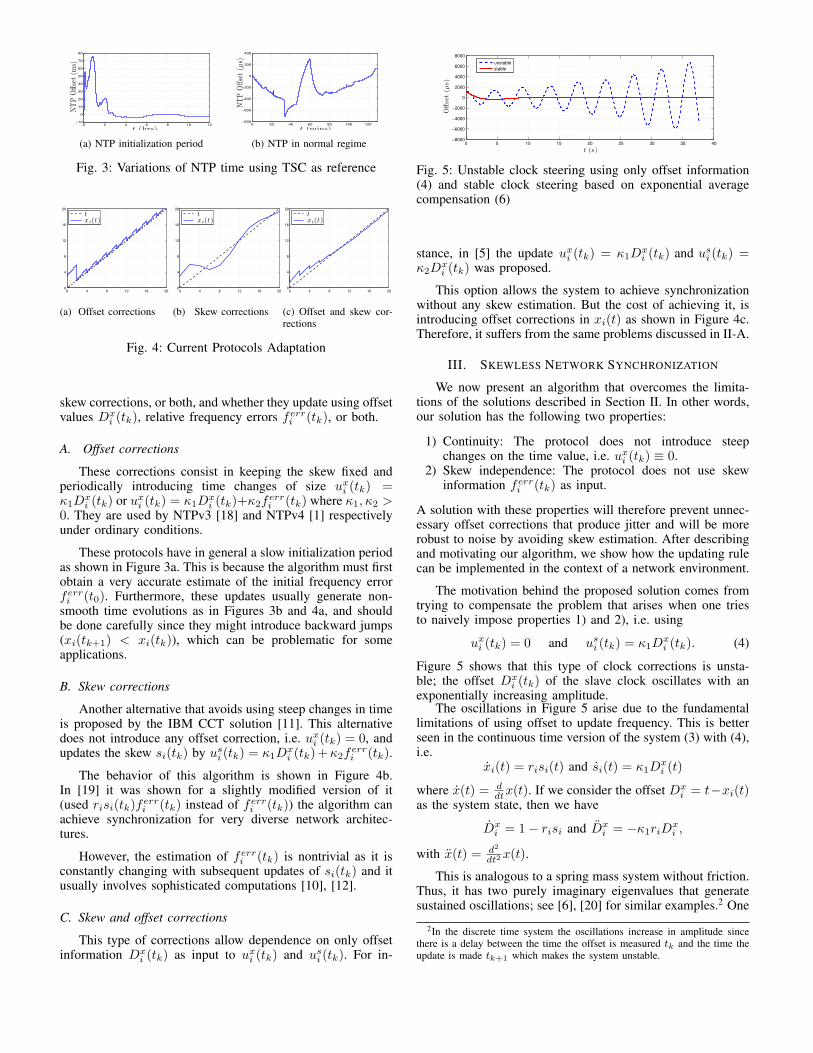
(a) NTP initialization period

0 20 40 60 80 100 120−800

−600

−400

−200

0

200

400

t (mins)

NTP

Offs

et(µ

s)

(b) NTP in normal regime

Fig. 3: Variations of NTP time using TSC as reference

0 4 8 12 16 200

4

8

12

16

20

txi(t)

(a) Offset corrections

0 4 8 12 16 200

4

8

12

16

20

txi(t)

(b) Skew corrections

0 4 8 12 16 200

4

8

12

16

20

txi(t)

(c) Offset and skew cor-rections

Fig. 4: Current Protocols Adaptation

skew corrections, or both, and whether they update using offsetvalues Dx

i (tk), relative frequency errors ferri (tk), or both.

A. Offset corrections

These corrections consist in keeping the skew fixed andperiodically introducing time changes of size uxi (tk) =κ1D

xi (tk) or uxi (tk) = κ1D

xi (tk)+κ2f

erri (tk) where κ1, κ2 >

0. They are used by NTPv3 [18] and NTPv4 [1] respectivelyunder ordinary conditions.

These protocols have in general a slow initialization periodas shown in Figure 3a. This is because the algorithm must firstobtain a very accurate estimate of the initial frequency errorferri (t0). Furthermore, these updates usually generate non-smooth time evolutions as in Figures 3b and 4a, and shouldbe done carefully since they might introduce backward jumps(xi(tk+1) < xi(tk)), which can be problematic for someapplications.

B. Skew corrections

Another alternative that avoids using steep changes in timeis proposed by the IBM CCT solution [11]. This alternativedoes not introduce any offset correction, i.e. uxi (tk) = 0, andupdates the skew si(tk) by usi (tk) = κ1D

xi (tk) +κ2f

erri (tk).

The behavior of this algorithm is shown in Figure 4b.In [19] it was shown for a slightly modified version of it(used risi(tk)ferri (tk) instead of ferri (tk)) the algorithm canachieve synchronization for very diverse network architec-tures.

However, the estimation of ferri (tk) is nontrivial as it isconstantly changing with subsequent updates of si(tk) and itusually involves sophisticated computations [10], [12].

C. Skew and offset corrections

This type of corrections allow dependence on only offsetinformation Dx

i (tk) as input to uxi (tk) and usi (tk). For in-

0 5 10 15 20 25 30 35 40−8000

−6000

−4000

−2000

0

2000

4000

6000

8000

t (s)

Offset(µ

s)

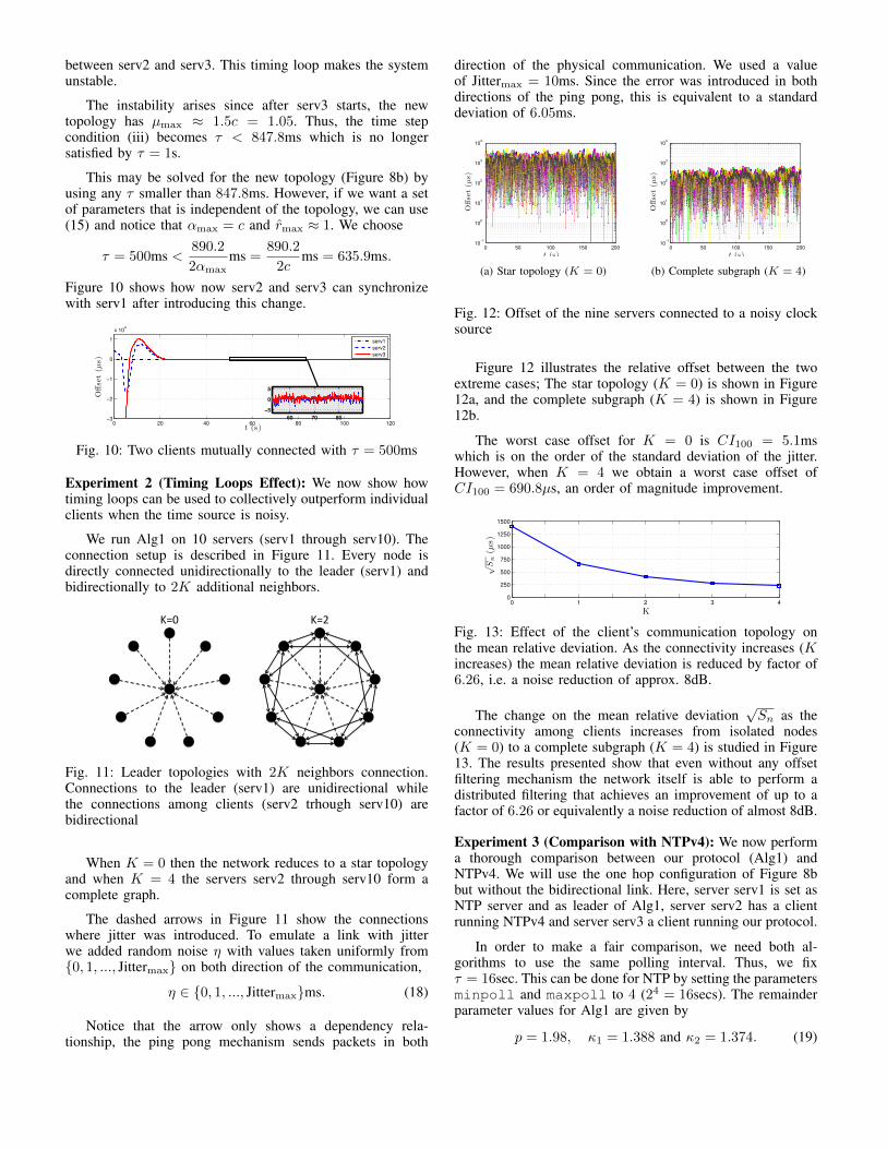
unstable

stable

Fig. 5: Unstable clock steering using only offset information(4) and stable clock steering based on exponential averagecompensation (6)

stance, in [5] the update uxi (tk) = κ1Dxi (tk) and usi (tk) =

κ2Dxi (tk) was proposed.

This option allows the system to achieve synchronizationwithout any skew estimation. But the cost of achieving it, isintroducing offset corrections in xi(t) as shown in Figure 4c.Therefore, it suffers from the same problems discussed in II-A.

III. SKEWLESS NETWORK SYNCHRONIZATION

We now present an algorithm that overcomes the limita-tions of the solutions described in Section II. In other words,our solution has the following two properties:

1) Continuity: The protocol does not introduce steepchanges on the time value, i.e. uxi (tk) ≡ 0.

2) Skew independence: The protocol does not use skewinformation ferri (tk) as input.

A solution with these properties will therefore prevent unnec-essary offset corrections that produce jitter and will be morerobust to noise by avoiding skew estimation. After describingand motivating our algorithm, we show how the updating rulecan be implemented in the context of a network environment.

The motivation behind the proposed solution comes fromtrying to compensate the problem that arises when one triesto naively impose properties 1) and 2), i.e. using

uxi (tk) = 0 and usi (tk) = κ1Dxi (tk). (4)

Figure 5 shows that this type of clock corrections is unsta-ble; the offset Dx

i (tk) of the slave clock oscillates with anexponentially increasing amplitude.

The oscillations in Figure 5 arise due to the fundamentallimitations of using offset to update frequency. This is betterseen in the continuous time version of the system (3) with (4),i.e.

xi(t) = risi(t) and si(t) = κ1Dxi (t)

where x(t) = ddtx(t). If we consider the offset Dx

i = t−xi(t)as the system state, then we have

Dxi = 1− risi and Dx

i = −κ1riDxi ,

with x(t) = d2

dt2x(t).

This is analogous to a spring mass system without friction.Thus, it has two purely imaginary eigenvalues that generatesustained oscillations; see [6], [20] for similar examples.2 One

2In the discrete time system the oscillations increase in amplitude sincethere is a delay between the time the offset is measured tk and the time theupdate is made tk+1 which makes the system unstable.

way to damp these oscillations in the spring-mass case is byadding friction. This implies adding a term that includes afrequency mismatch ferri (t) in our system, which is equivalentto the protocols of Section II-B, and therefore undesired.

However, there are other ways to damp these oscillationsusing passivity-based techniques from control theory [21],[22]. The basic idea is to introduce an additional state yi thatgenerates the desired friction to damp the oscillations.

Inspired by [21], we consider the exponentially weightedmoving average of the offset

yi(tk+1) = pDxi (tk) + (1− p)yi(tk). (5)

and update xi(tk) and si(tk) using:

uxi (tk) = 0 and usi (tk) = κ1Dx(tk)− κ2y(tk). (6)

Figure 5 shows how the proposed strategy is able to compen-sate the oscillations without needing to estimate the value offerri (tk). The stability of the algorithm will depend on howκ1, κ2 and p are chosen. A detailed specification of thesevalues is given in Section IV-B.

Finally, since we are interested in studying the effect oftiming loops, we move away from the client-server config-uration implicitly assumed in Section II and allow mutualor cyclic interactions among nodes. The interactions betweendifferent nodes is described by a graph G(V,E), where Vrepresents the set of n nodes (i ∈ V ) and E the set of directededges ij; ij ∈ E means node i can measure its offset withrespect to j, Dx

ij(tk) = xj(tk)− xi(tk).

Within this context, a natural extension of (5)-(6) is tosubstitute Dx

i (tk) with the weighted average of i’s neighborsoffsets. Thus, we propose the following algorithm to updatethe clocks in the network.

Algorithm 1 (Alg1): For each computer node i in the network,perform the following actions:

- Compute the time offsets (Dxij(tk)) from i to every neighbor

j at time tk.- Update the skew si(tk+1) and the moving average yi(tk+1)

at time tk+1 according to:

si(tk+1) =si(tk) + κ1∑j∈Ni

αijDxij(tk)− κ2yi(tk) (7a)

yi(tk+1) =p∑j∈Ni

αijDxij(tk) + (1− p)yi(tk) (7b)

whereNi represents the set of neighbors of i and the weightsαij are positive.

Using this algorithm, many servers can affect the finalfrequency of the system. Thus, when the system synchronizes,we have

xi(tk) = r∗(tk − t0) + x∗ i ∈ V. (8)

r∗ and x∗ are possibly different from their ideal values 1 andt0. Their final values depend on the initial condition of alldifferent clocks as well as the topology, which we assume tobe a connected graph in this paper.

IV. ANALYSIS

We now analyze the asymptotic behavior of system (7) andprovide a necessary and sufficient condition on the parametervalues that guarantee its convergence to (8). The techniquesused are drawn from the control literature, e.g. [5] and [19],yet its application in our case is nontrivial.

Notation: We use 0m×n (1m×n) to denote the matricesof all zeros (ones) within Rm×n and 0n (1n) to denotethe column vectors of appropriate dimensions. In ∈ Rn×nrepresents the identity matrix. Given a matrix A ∈ Rn×n withJordan normal form A = PJP−1, let nA ≤ n denote the totalnumber of Jordan blocks Jl with l ∈ I(A) := {1, ..., nA}.We use µl(A), l ∈ {1, . . . , n} or just µ(A) to denote theeigenvalues of A, and order them decreasingly |µ1(A)| ≥· · · ≥ |µn(A)|. Finally, AT is the transpose of A, Aij is theelement of the ith row and jth column of A and ai is the ithelement of the column vector a, i.e. a = [ai]

T .

It is more convenient for the analysis to use a vector formrepresentation of (7) given by

zk+1 = Azk (9)

where zk := [x(tk)T s(tk)T y(tk)T ]T ∈ R3n,

A :=

[In τR 0n×n−κ1L In −κ2Inp(−L) 0n×n (1− p)In

]∈ R3n×3n,

R ∈ Rn×n is the diagonal matrix with elements ri and L ∈Rn×n is the Laplacian matrix associated with G(V,E),

Lii = αii :=∑j∈Ni

αij and Lij =

{−αij if ij ∈ E,0 otherwise.

The convergence analysis of this section is done in twostages. First, we provide necessary and sufficient conditionsfor synchronization in terms of the eigenvalues of A (SectionIV-A) and then use Hermite-Biehler Theorem [23] to relatethese eigenvalues with the parameter values that can bedirectly used in practice (Section IV-B). All the proof detailsare included in the appendix for interested readers.

A. Asymptotic Behavior

We start by studying the asymptotic behavior of (9). Thatis, we are interested in finding under what conditions the seriesof elements {xi(tk)} converge to (8) as tk goes to infinity.

Consider the Jordan normal form [24] of

A := [ζ1 ... ζ3n] J [η1 ... η3n]T

where J = blockdiag(Jl)l∈I(A), ζi and ηi are the right andleft generalized eigenvectors of A such that

ζTi ηj =

{1 if j = i,0 otherwise.

The crux of the analysis comes from understanding the rela-tionship between the multiplicity of the eigenvalue µ(A) = 1and the eigenvalue µ(L) = 0, and their corresponding eigen-vectors. This is captured in the next two lemmas.

Lemma 1 (Eigenvalues of A and Multiplicity of µ(A) = 1):A has an eigenvalue µ(A) = 1 with multiplicity 2 if and onlyif the graph G(V,E) is connected, κ1 6= κ2 and p > 0.

Furthermore, µl(A) are the roots of

gl(λ) := (λ− 1)2(λ− 1 + p) + [(λ− 1)κ1 +κ2−κ1]νl (10)

where νl = µl(τLR) and satisfies

νn = 0 < |νl| for l ∈ {1, . . . , n− 1}. (11)

Lemma 2 (Jordan Chains of µ(A) = 1 and µ(A) = 1− p):Under the conditions of Lemma 1 the right and left Jordanchains, (ζ1, ζ2) and (η2, η1) respectively, associated withµ(A) = 1 and the eigenvectors ζ3 and η3 associated withµ(A) = 1− p are given by

[ζ1 ζ2 ζ3] =

1n 1n − τκ2

p2 1n

0n(R−11n)

τκ2

p R−11n

0n 0n R−11n

and (12)

[η1 η2 η3] = γ

R−1ξ 0n 0n−τξ ξ 0n

τκ2( 1p + 1

p2 )ξ −κ2

p ξ ξ

(13)

where ξ is the unique normalized left eigenvector of µ(L) = 0(∑ni=1 ξi = 1) and γ is the ξi-weighted harmonic mean of ri,

i.e. 1γ = 1TnR

−1ξ =∑ni=1

ξiri.

The proof of Lemmas 1 and 2 can be found in theAppendices A and B. We now proceed to state our mainconvergence result.

Theorem 1 (Convergence): The algorithm (9) achievessynchronization for any initial conditions if and only if thegraph G(V,E) is connected, κ1 6= κ2, p > 0 and |µl(A)| < 1whenever µl(A) 6= 1. Moreover, whenever the system syn-chronizes, we have

x∗ = γ

n∑i=1

ξi

(1

rixi(t0) + τ

κ2p2yi(t0)

), and (14a)

r∗ = γ

n∑i=1

ξi(si(t0)− κ2pyi(t0)). (14b)

Theorem 1 provides an analytical tool to understand theinfluence of the different nodes of the graph in the final offsetx∗ and frequency r∗. For example, suppose that we know thatnode 1 has perfect knowledge of its own frequency (r1) andthe UTC time at t = t0 (x1(t0) = t0), and configure thenetwork such that node 1 is the unique leader like the topnode in Figures 6a and 6c. It is easy to show that ξ1 = 1 andξi = 0 ∀i 6= 1. Then, using (14a)-(14b) and definition of γwe can see that γ = r1 and

x∗ = x1(t0) + r1τκ2p2y1(t0) and r∗ = r1s1(t0)− r1κ2

py1(t0).

However, since node 1 knows r1 and t0, it can choosex1(t0) = t0, s1(t0) = 1

r1and y1(t0) = 0. Thus, we obtain

x∗ = t0 and r∗ = 1 which implies by (8) that every node in thenetwork will end up with xi(t) = t. In other words, Theorem1 allows us to understand how the information propagates andhow we can guarantee that every server will converge to thedesired time. Notice that the initial condition used for server1 is equivalent to assuming that server 1 is a reliable sourceof UTC like an atomic clock for instance.

(a)   (b)   (c)  

Fig. 6: Graphs with real eigenvalue Laplacians

B. Necessary and sufficient conditions for synchronization

We now provide necessary and sufficient conditions interms of explicit parameter values (κ1, κ2 ,τ and p) for Theo-rem 1 to hold. We will restrict our attention to graphs that haveLaplacian matrices with real eigenvalues. This includes forexample trees (Figure 6a), symmetric graphs with αij = αji(Figure 6b) and symmetric graphs with a leader (Figure 6c).

The proof consists on studying the Schur stability ofgl(λ) and has several steps. We first perform a change ofvariable that maps the unit circle onto the left half-plane. Thistransforms the problem of studying the Schur stability intoa Hurwitz stability problem which is solved using Hermite-Biehler Theorem.

Theorem 2 (Hurwitz Stability (Hermite-Beihler) [23]):Given the polynomial P (s) = ans

n + ... + a0, let P r(ω)and P i(ω) be the real and imaginary part of P (jω),i.e. P (jω) = P r(ω) + jP i(ω). Then P (s) is a Hurwitzpolynomial if and only if

1) anan−1 > 0 and 2)

2) The zeros of P r(ω) and P i(ω) are all simple and realand interlace as ω runs from −∞ to +∞.

We now determine the proper parameter values that guar-antee synchronization.

Theorem 3 (Parameter Values for Synchronization):Given a connected graph G(V,E) such that the correspondingLaplacian matrix L has real eigenvalues. The system (9)achieves synchronization if and only if

(i) |1− p| < 1 or equivalently 2 > p > 0

(ii) 2κ1

3p > κ1 − κ2 > 0 and (iii) τ < p(κ2−p(κ1−κ2))µmax(κ1−p(κ1−κ2))2

where µmax is the largest eigenvalue of LR.

Even though µmax depends on ri which is in generalunknown, it is easy to show that µl(LR) ≤ rmaxµl(L) wherermax is an upper bound of the maximum rate deviation ri.Furthermore, using Greshgorin’s circle theorem, it is easy toshow that µmax(L) ≤ 2αmax := 2 maxi αii. Therefore, if weset

τ <p(κ2 − δκp)

2αmaxrmax(κ1 − δκp)2(15)

convergence is guaranteed for every connected graph withreal eigenvalues.

V. EXPERIMENTS

To test our solution and analysis, we implement an asyn-chronous version of Algorithm 1 (Alg1) in C using the IBM

Fig. 7: Testbed of IBM BladeCenter blade servers

CCT solution as our code base. Every node perform its ownmeasurements and updates every τ seconds using (7), but notnecessarily at the same instants tk.

Our program reads the TSC counter directly using therdtsc assembly instruction to minimize reading latenciesand maintains a virtual clock that can be directly updated.The list of neighbors is read from a configuration file andwhenever there is no neighbor, the program follows the localLinux clock. Finally, offset measurements are taken using animproved ping pong mechanism proposed in [11].

We run our skewless protocol in a cluster of IBM Blade-Center LS21 servers with two AMD Opteron processors of2.40GHz, and 16GB of memory. As shown in Figure 7,the servers serv1-serv10 are used to run the protocol. Theoffset measurements are taken through a Gigabit Ethernetswitch. Server serv0 is used as a reference node and gatherstime information from the different nodes using a Cisco 4xInfiniBand Switch that supports up to 10Gbps between anytwo ports and up to 240Gbps of aggregate bandwidth. Thisminimizes the error induced by the data collecting process.

We use this testbed to validate the analysis in SectionIV. First, we illustrate the effect of different parameters andanalyze the effect of the network configuration on convergence(Experiment 1). Then we present a series of configurationsthat demonstrate how connectivity between clients is usefulin reducing the jitter of a noisy clock source (Experiment2). And finally, we compare the performance of our protocolwith respect to NTP version 4 (Experiment 3) and IBM CCT(Experiment 4).

We will use several performance metrics to evaluate Alg1.For instance, the mean relative deviation from the leaderwhich is defined as the root mean square of the nodes offsetwith respect to the leader, i.e.

√Sn with

Sn =1

n− 1

n∑i=2

⟨(xi − x1)2

⟩, (16)

where < · > amounts to the sample average. We will also usethe 99% Confidence Interval CI99 and the maximum offset(CI100) as metrics of accuracy. For example, if CI99 = 10µs,then the 99% of the offset samples will be within 10µs of theleader.

Unless explicitly stated, the default parameter values are

p = 0.99, κ1 = 1.1, κ2 = 1.0 and αij =c

|Ni|. (17)

The scalar c is a commit or gain factor that will allow us tocompensate the effect of τ . Notice that by definition of αij ,αii = c for every node that is not the leader.

Moreover, these values immediately satisfy (i) and (ii) ofTheorem 3 since 1−p = 0.01 and 2κ1

3p = 0.7407 > κ1−κ2 =0.1. The remaining condition can be satisfied by modifying τor equivalently c. Here, we choose to fix c = 0.7 which makescondition (iii)

τ <890.1

µmaxms.

For fixed polling interval τ , the stability of the system dependson the value of µmax, which is determined by the underlyingnetwork topology and the values of αij .

!"#$%& !"#$'& !"#$%&

!"#$(&

!"#$'&)*+& ),+&

Fig. 8: Effect of topology on convergence: (a) Client-serverconfiguration; (b) Two clients connected to server and mutu-ally connected.

Experiment 1 (Convergence): We first consider the clientserver configuration described in Figure 8a with a time stepτ = 1s. In this configuration µmax ≈ c = 0.7 and thereforecondition (iii) becomes τ < 1.2717s. Figure 9a shows theoffset between serv1 (the leader) and serv2 (the client) inmicroseconds. There we can see how serv2 gradually updatess2(tk) until the offset becomes insignificant.

0 20 40 60 80 100 120 140 160 180 200−3

−2.5

−2

−1.5

−1

−0.5

0

0.5

1

1.5x 10

4

t (s)

Offset(µ

s)

serv1

serv2

100 120 140

−10

0

10

(a) Client server configuration withτ = 1s. The client converges and thealgorithm is stable.

0 20 40 60 80 100 120−1.5

−1

−0.5

0

0.5

1

1.5x 10

5

t (s)

Offset(µ

s)

serv1

serv2

serv3

(b) Two clients mutually connectedwith τ = 1s. The algorithm becomesunstable.

Fig. 9: Loss of stability by change in the network topology

Figure 9a tends to suggest that the set of parameters givenby (17) and τ = 1s are suitable for deployment on the servers.This is in fact true provided that network is a directed tree asin Figure 6a. The intuition behind this fact is that in a tree,each client connects only to one server. Thus, those connectedto the leader will synchronize first and then subsequent layerswill follow.

However, once loops appear in the network, there is nolonger a clear dependency since two given nodes can mutuallyget information from each other. This type of dependencymight make the algorithm unstable. Figure 9b shows anexperiment with the same configuration as Figure 9a in whichserv2 synchronizes with serv1 until a third server (serv3)appears after 60s. At that moment the system is reconfiguredto have the topology of Figure 8b introducing a timing loop

between serv2 and serv3. This timing loop makes the systemunstable.

The instability arises since after serv3 starts, the newtopology has µmax ≈ 1.5c = 1.05. Thus, the time stepcondition (iii) becomes τ < 847.8ms which is no longersatisfied by τ = 1s.

This may be solved for the new topology (Figure 8b) byusing any τ smaller than 847.8ms. However, if we want a setof parameters that is independent of the topology, we can use(15) and notice that αmax = c and rmax ≈ 1. We choose

τ = 500ms <890.2

2αmaxms =

890.2

2cms = 635.9ms.

Figure 10 shows how now serv2 and serv3 can synchronizewith serv1 after introducing this change.

0 20 40 60 80 100 120−3

−2

−1

0

1

x 104

t (s)

Offset(µ

s)

serv1

serv2

serv3

60 70 80

−5

0

5

Fig. 10: Two clients mutually connected with τ = 500ms

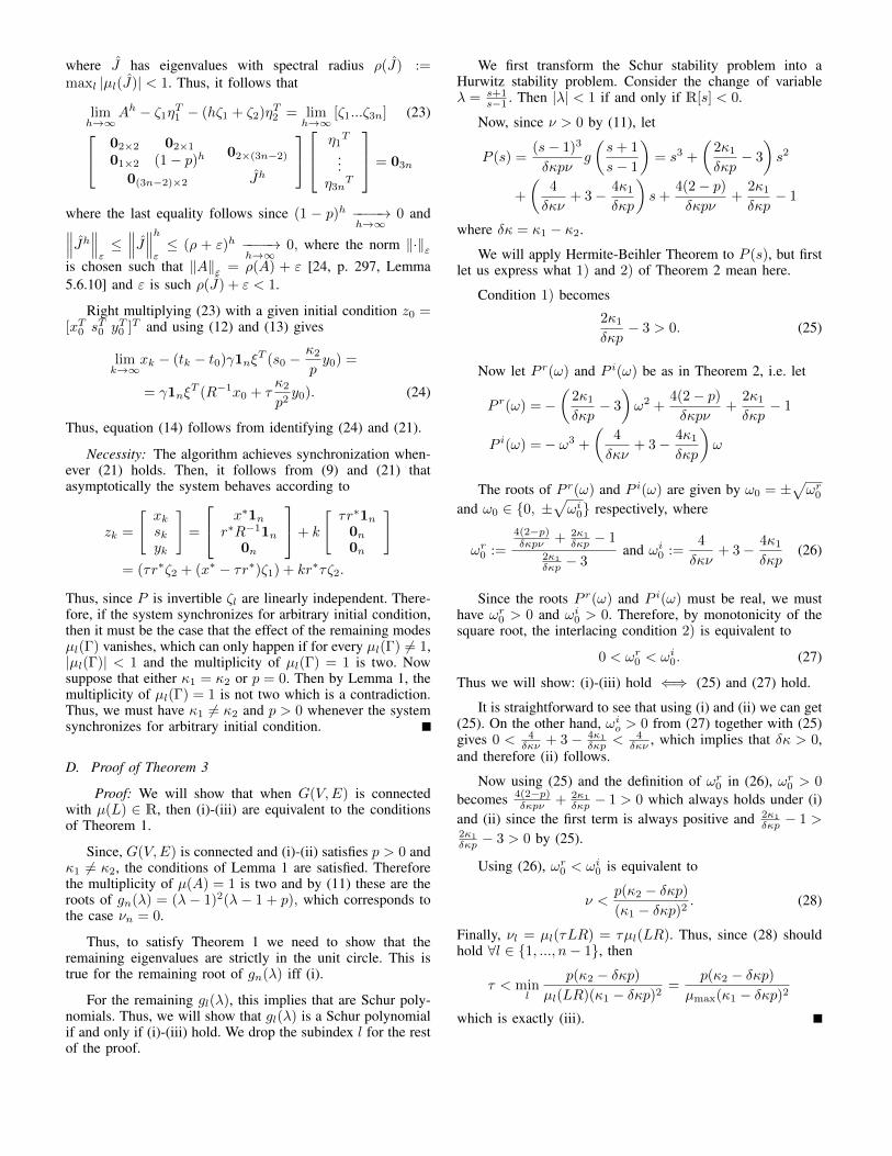
Experiment 2 (Timing Loops Effect): We now show howtiming loops can be used to collectively outperform individualclients when the time source is noisy.

We run Alg1 on 10 servers (serv1 through serv10). Theconnection setup is described in Figure 11. Every node isdirectly connected unidirectionally to the leader (serv1) andbidirectionally to 2K additional neighbors.

K=0   K=2  

Fig. 11: Leader topologies with 2K neighbors connection.Connections to the leader (serv1) are unidirectional whilethe connections among clients (serv2 trhough serv10) arebidirectional

When K = 0 then the network reduces to a star topologyand when K = 4 the servers serv2 through serv10 form acomplete graph.

The dashed arrows in Figure 11 show the connectionswhere jitter was introduced. To emulate a link with jitterwe added random noise η with values taken uniformly from{0, 1, ..., Jittermax} on both direction of the communication,

η ∈ {0, 1, ..., Jittermax}ms. (18)

Notice that the arrow only shows a dependency rela-tionship, the ping pong mechanism sends packets in both

direction of the physical communication. We used a valueof Jittermax = 10ms. Since the error was introduced in bothdirections of the ping pong, this is equivalent to a standarddeviation of 6.05ms.

0 50 100 150 20010

−1

100

101

102

103

104

t (s)

Offset(µ

s)

(a) Star topology (K = 0)

0 50 100 150 20010

−1

100

101

102

103

104

t (s)

Offset(µ

s)

(b) Complete subgraph (K = 4)

Fig. 12: Offset of the nine servers connected to a noisy clocksource

Figure 12 illustrates the relative offset between the twoextreme cases; The star topology (K = 0) is shown in Figure12a, and the complete subgraph (K = 4) is shown in Figure12b.

The worst case offset for K = 0 is CI100 = 5.1mswhich is on the order of the standard deviation of the jitter.However, when K = 4 we obtain a worst case offset ofCI100 = 690.8µs, an order of magnitude improvement.

0 1 2 3 40

250

500

750

1000

1250

1500

K

√Sn(µ

s)

Fig. 13: Effect of the client’s communication topology onthe mean relative deviation. As the connectivity increases (Kincreases) the mean relative deviation is reduced by factor of6.26, i.e. a noise reduction of approx. 8dB.

The change on the mean relative deviation√Sn as the

connectivity among clients increases from isolated nodes(K = 0) to a complete subgraph (K = 4) is studied in Figure13. The results presented show that even without any offsetfiltering mechanism the network itself is able to perform adistributed filtering that achieves an improvement of up to afactor of 6.26 or equivalently a noise reduction of almost 8dB.

Experiment 3 (Comparison with NTPv4): We now performa thorough comparison between our protocol (Alg1) andNTPv4. We will use the one hop configuration of Figure 8bbut without the bidirectional link. Here, server serv1 is set asNTP server and as leader of Alg1, server serv2 has a clientrunning NTPv4 and server serv3 a client running our protocol.

In order to make a fair comparison, we need both al-gorithms to use the same polling interval. Thus, we fixτ = 16sec. This can be done for NTP by setting the parametersminpoll and maxpoll to 4 (24 = 16secs). The remainderparameter values for Alg1 are given by

p = 1.98, κ1 = 1.388 and κ2 = 1.374. (19)

Figure 14a shows the time differences between the clientsrunning NTPv4 and Alg1 (serv2 and serv3) , and the leader(serv1) over a period of 30 hours. It can be seen that Alg1is able to track serv1’s clock keeping an offset smaller than10µs for most of the time while NTPv4 incurs in larger offsetsduring the same period of time. This difference is producedby the fact that Alg1 is able to react more rapidly to frequencychanges while NTPv4 incurs in more offset corrections thatgenerate larger jitter.

0 5 10 15 20 25 30−30

−20

−10

0

10

20

30

t (hours)

Offset(µ

s)

NTPv4

Alg1

(a) Offset values of NTPv4 and Alg1for a period of 30 hours.

10−2

10−1

100

101

102

0

0.1

0.2

0.3

0.4

0.5

0.6

0.7

0.8

0.9

1

Offset (µs)

CDF

NTPv4

Alg1

(b) Cummulative Distribution Func-tion

Fig. 14: Performance evaluation between our solution (Alg1)and NTPv4

A more detailed and comprehensive analysis is presentedin Figure 14b where we plot the Cumulative DistributionFunction (CDF) of the offset samples. That is, the fractionof samples whose time offset is smaller than a specificvalue. Using Figure 14b we compute the corresponding 99%confidence intervals (CI99)

Alg1 achieves a performance of√Sn = 3.1µs, CI99 =

9.5µs and a maximum offset of CI100 = 15.9µs, while NTPv4obtains

√Sn = 8.1µs, CI99 = 21.8µs and a maximum offset

of CI100 = 28.0µs. Thus, not only Alg1 achieves a reductionof√Sn by a factor of 2.6 (−4.2dB) with respect to NTPv4,

but it also obtains smaller confidence intervals and maximumoffset values.

0 0.5 1 1.5 2 2.5 3 3.5 4 4.510

−1

100

101

102

103

104

t (hours)

Offset(µ

s)

NTPv4

Alg1

Fig. 15: Offset values of NTPv4 and Alg1 after a 25ms offsetintroduced in serv1.

Finally, we investigate the speed of convergence. Startingfrom both clients synchronized to server serv1, we introducea 25ms offset. Figure 15 shows how Alg1 is able to convergeto a 20µs range within one hour while NTPv4 needs 4.5hoursto achieve the same synchronization precision.

Experiment 4 (Comparison with IBM CCT): We nowproceed to compare the performance of Alg1 with respect toIBM CCT. Notice that unlike IBM CCT, our solution doesnot perform any previous filtering of the offset samples, thefiltering is performed instead by calibrating the parameterswhich mostly depend on the polling interval τ chosen. Herewe use c = 0.70, τ = 250ms, κ1 = 0.1385, κ2 = 0.1363 andp = 0.62.

In Figure 16a we present the mean relative deviation√Sn for two clients connected directly to the leader as

the jitter is increased from Jittermax = 0µs (no jitter) toJittermax = 160µs with a granularity of 1µs. The worst caseoffset is shown in Figure 16b. Each data point is computedusing a sample run of 250 seconds.

Our algorithm consistently outperforms IBM CCT in termsof both

√Sn and worst case offset. The performance im-

provement is due to two reasons. Firstly, the noise filter usedby the IBM CCT algorithm is tailored for noise distributionsthat are mostly concentrated close to zero with sporadic largeerrors. However, it does not work properly in cases where thedistribution is more homogeneous as in this case. Secondly,by choosing δκ = κ1−κ2 = 0.002� 1 the protocol becomesvery robust to offset errors.

10 20 30 40 50 60 70 80 90100 1600

1

2

3

4

5

6

7

8

9

Jittermax (µs)

√Sn(µ

s)

Alg1

IBM CCT

(a) Mean relative deviation√Sn

10 20 30 40 50 60 70 80 90100 1600

5

10

15

20

25

30

35

Jittermax (µs)

CI 1

00(µ

s)

Alg1

IBM CCT

(b) Maximum offset

Fig. 16: Performance evaluation between our solution (Alg1)and IBM CCT

VI. CONCLUSION

This paper presents a clock synchronization protocol thatis able to synchronize networked nodes without explicit es-timation of the clock skews and steep corrections on thetime. Unlike current standards, our protocol is guaranteedto converge even in the presence of timing loops whichallows different clients to share timing information and evencollectively outperform individual clients. We implementedour solution on a cluster of IBM BladeCenter servers and em-pirically verified our predictions and our protocol’s supremacyover several existing solutions.

REFERENCES

[1] D. Mills, “Network time protocol version 4 reference and implemen-tation guide,” University of Delaware, Tech. Rep. 06-06-1, Jun. 2006.

[2] A. Sobeih et al., “Almost peer-to-peer clock synchronization,” Paralleland Distributed Processing Symposium, International, p. 21, 2007.

[3] “IEEE standard for a precision clock synchronization protocol fornetworked measurement and control systems,” pp. 1 –269, 2008.

[4] D. Veitch, J. Ridoux, and S. B. Korada, “Robust synchronizationof absolute and difference clocks over networks,” IEEE/ACM Trans.Netw., vol. 17, no. 2, pp. 417–430, Apr. 2009.

[5] R. Carli and S. Zampieri, “Networked clock synchronization based onsecond order linear consensus algorithms,” in Decision and Control(CDC), 2010 49th IEEE Conference on, Dec. 2010, pp. 7259 –7264.

[6] E. Mallada and A. Tang, “Distributed clock synchronization: Joint fre-quency and phase consensus,” in Decision and Control and EuropeanControl Conference (CDC-ECC), 2011 50th IEEE Conference on, Dec.2011, pp. 6742 –6747.

[7] J. Ridoux, D. Veitch, and T. Broomhead, “The case for feed-forward clock synchronization,” IEEE/ACM Transactions on Network-ing, vol. 20, no. 1, pp. 231–242, 2012.

[8] J. C. Corbett et al., “Spanner: Google’s globally-distributed database,”in Proceedings of the 10th USENIX conference on OperatingSystems Design and Implementation, ser. OSDI’12. Berkeley, CA,USA: USENIX Association, 2012, pp. 251–264. [Online]. Available:http://dl.acm.org/citation.cfm?id=2387880.2387905

[9] B. Sundararaman, U. Buy, and A. D. Kshemkalyani, “Clock synchro-nization for wireless sensor networks: a survey,” Ad Hoc Networks,vol. 3, no. 3, pp. 281–323, 2005.

[10] H. Kim, X. Ma, and B. Hamilton, “Tracking low-precision clocks withtime-varying drifts using kalman filtering,” Networking, IEEE/ACMTransactions on, vol. 20, no. 1, pp. 257 –270, Feb. 2012.

[11] S. Froehlich et al., “Achieving precise coordinated cluster time in acluster environment,” in Precision Clock Synchronization for Mea-surement, Control and Communication, 2008. ISPCS 2008. IEEEInternational Symposium on, Sep. 2008, pp. 54 –58.

[12] L. Zhang, Z. Liu, and C. Honghui Xia, “Clock synchronization algo-rithms for network measurements,” in INFOCOM 2002. Twenty-FirstAnnual Joint Conference of the IEEE Computer and CommunicationsSocieties. Proceedings. IEEE, vol. 1, 2002, pp. 160 – 169 vol.1.

[13] J. Elson, L. Girod, and D. Estrin, “Fine-grained network time synchro-nization using reference broadcasts,” SIGOPS Oper. Syst. Rev., vol. 36,no. SI, pp. 147–163, 2002.

[14] D. Hunt, G. Korniss, and B. Szymanski, “Network synchronization ina noisy environment with time delays: Fundamental limits and trade-offs,” Physical Review Letters, vol. 105, no. 6, p. 068701, 2010.

[15] H. Marouani and M. R. Dagenais, “Internal clock drift estimation incomputer clusters,” J. Comp. Sys., Netw., and Comm., vol. 2008, pp.9:1–9:7, Jan. 2008.

[16] S. Moon, P. Skelly, and D. Towsley, “Estimation and removal ofclock skew from network delay measurements,” in INFOCOM ’99.Eighteenth Annual Joint Conference of the IEEE Computer and Com-munications Societies. Proceedings. IEEE, vol. 1, Mar. 1999, pp. 227–234 vol.1.

[17] M. Lemmon, J. Ganguly, and L. Xia, “Model-based clock synchroniza-tion in networks with drifting clocks,” in Dependable Computing, 2000.Proceedings. 2000 Pacific Rim International Symposium on, 2000, pp.177 –184.

[18] D. Mills, “Network time protocol (version 3) specification, implemen-tation and analysis,” 1992.

[19] D. Xie and S. Wang, “Consensus of second-order discrete-time multi-agent systems with fixed topology,” Journal of Mathematical Analysisand Applications, 2011.

[20] E. Mallada and F. Paganini, “Stability of node-based multipath routingand dual congestion control,” in Decision and Control, 2008. CDC2008. 47th IEEE Conference on. IEEE, 2008, pp. 1398–1403.

[21] W. Ren and R. W. Beard, “Consensus algorithms for double-integratordynamics,” Distributed Consensus in Multi-vehicle Cooperative Con-trol: Theory and Applications, pp. 77–104, 2008.

[22] W. Ren and R. Beard, Distributed consensus in multi-vehicle cooper-ative control: theory and applications. Springer, 2008.

[23] S. Bhattacharyya, H. Chapellat, and L. Keel, Robust control. Prentice-Hall Upper Saddle River, New Jersey, 1995.

[24] R. Horn and C. Johnson, Matrix analysis. Cambridge Univ Pr, 1990.

APPENDIX

A. Proof of Lemma 1

Proof: We first compute the characteristic polynomial

det(λI3n −A) =

∣∣∣∣∣ (λ− 1)In −τR 0n×nκ1L (λ− 1)In κ2InpL 0 (λ− 1 + p)In

∣∣∣∣∣= (λ− 1)n

∣∣∣∣ (λ− 1)In + τκ1

λ−1LR κ2Inτpλ−1LR (λ− 1 + p)In

∣∣∣∣= det

((λ− 1)2(λ− 1 + p)In + [(λ− 1)κ1

+(κ2 − κ1)]τLR) =

n∏l=1

gl(λ),

where gl(λ) is as defined in (10) and we have iterativelyuse the determinant property of block matrices det(A) =

det(A11) det(A\A11) where A =

[A11 A12

A21 A22

]and

A\A11 = A22 − A21A−111 A12 is the Schur complement of

A11 [24].

Thus, λ = 1 is a double root of the characteristic polyno-mial if and only if κ1 6= κ2, p > 0 and τLR has a simple zeroeigenvalue, i.e. (11). Now, since R is nonsingular (11) musthold for the eigenvalues of L as well, which is in fact true ifand only if the directed graph G(V,E) is connected [19].

B. Proof of Lemma 2

Proof: We start by computing the right Jordan chain. Bydefinition of ζ1, (A− I)ζ1 = 0n. Thus, if ζ1 = [xT sT yT ]T ,then the following system of equations must be satisfied

τRs = 0n (a), − κ1Lx− κ2y = 0n (b) and−pLx− py = 0n (c). (20)

Equation (20a) implies s = 0. Now, since p > 0, (20c)implies Lx = −y, which when substituted in (20b) gives(κ2 − κ1)y = 0n. Thus, since κ1 6= κ2, y = 0n andx ∈ ker(L). By choosing x = α11n (for some α1 6= 0)we obtain ζ1 = α1

[1Tn 0Tn 0Tn

]T.

Notice that the computation also shows that ζ1 is theunique eigenvector of µ(A) = 1 which implies that thereis only one Jordan block of size 2. The second member ofthe chain, ζ2, and ζ3 can be computed similarly by solving(A− In)ζ2 = ζ1 and (A− (1− p)In)ζ3 = 0n. This gives

ζ2 =

α21nα1

τ R−11n0n

and ζ3 = α3

− τκ2

p2 1nκ2

p R−11n

R−11n

.In computing ζ3, we obtain Lx = 0 and Rx = − τps = −κ2τ

p2 y.ζ3 follows by taking y = α3R

−11n.

The vectors η1, η2 and η3 can be solved inthe same way using ηT2 (A − I) = 0Tn , ηT1 (A −I) = ηT2 and ηT3 (A − (1 − p)I) = 0Tn . This

gives η1 =[β2

τ R−1ξT β1ξ

T (−κ2

p β1 + κ2

p2 β2)ξT]T

, η2 =

β2

[0Tn ξ

T κ2

p ξT]T

and η3 = β3[0Tn 0Tn ξ

T]T. We set

α1 = α2 = α3 = 1; this can be done WLOG provided we stillsatisfy ηTl ζl = 1 and ηTl ζh = 0 for l 6= h. Finally, ηT1 ζ1 = 1givesβ2 = γτ , ηT3 ζ3 = 1 gives β3 = γ and ηT1 ζ2 = 0 givesβ1 = −β2 = −γτ .

C. Proof of Theorem 1

Proof: We first notice that whenever x(tk) approaches(8) then

limh→∞

x(th)− r∗1n(th − t0) = x∗1n (21)Sufficiency: Since we are under the assumptions of Lem-

mas 1 and 2 we know that µ(A) = 1 has multiplicity 2 anda Jordan chain of size 2. Thus, the Jordan normal form of Ais

A = [ζ1...ζ3n]

1 1 00 1 00 0 1− p

03×3(n−1)

03(n−1)×3 J

η1

T

...η3n

T

(22)

where J has eigenvalues with spectral radius ρ(J) :=maxl |µl(J)| < 1. Thus, it follows that

limh→∞

Ah − ζ1ηT1 − (hζ1 + ζ2)ηT2 = limh→∞

[ζ1...ζ3n] (23) 02×2 02×101×2 (1− p)h 02×(3n−2)

0(3n−2)×2 Jh

η1

T

...η3n

T

= 03n

where the last equality follows since (1 − p)h −−−−→h→∞

0 and∥∥∥Jh∥∥∥ε≤∥∥∥J∥∥∥h

ε≤ (ρ + ε)h −−−−→

h→∞0, where the norm ‖·‖ε

is chosen such that ‖A‖ε = ρ(A) + ε [24, p. 297, Lemma5.6.10] and ε is such ρ(J) + ε < 1.

Right multiplying (23) with a given initial condition z0 =[xT0 sT0 yT0 ]T and using (12) and (13) gives

limk→∞

xk − (tk − t0)γ1nξT (s0 −

κ2py0) =

= γ1nξT (R−1x0 + τ

κ2p2y0). (24)

Thus, equation (14) follows from identifying (24) and (21).

Necessity: The algorithm achieves synchronization when-ever (21) holds. Then, it follows from (9) and (21) thatasymptotically the system behaves according to

zk =

[xkskyk

]=

x∗1nr∗R−11n

0n

+ k

[τr∗1n0n0n

]= (τr∗ζ2 + (x∗ − τr∗)ζ1) + kr∗τζ2.

Thus, since P is invertible ζl are linearly independent. There-fore, if the system synchronizes for arbitrary initial condition,then it must be the case that the effect of the remaining modesµl(Γ) vanishes, which can only happen if for every µl(Γ) 6= 1,|µl(Γ)| < 1 and the multiplicity of µl(Γ) = 1 is two. Nowsuppose that either κ1 = κ2 or p = 0. Then by Lemma 1, themultiplicity of µl(Γ) = 1 is not two which is a contradiction.Thus, we must have κ1 6= κ2 and p > 0 whenever the systemsynchronizes for arbitrary initial condition.

D. Proof of Theorem 3

Proof: We will show that when G(V,E) is connectedwith µ(L) ∈ R, then (i)-(iii) are equivalent to the conditionsof Theorem 1.

Since, G(V,E) is connected and (i)-(ii) satisfies p > 0 andκ1 6= κ2, the conditions of Lemma 1 are satisfied. Thereforethe multiplicity of µ(A) = 1 is two and by (11) these are theroots of gn(λ) = (λ− 1)2(λ− 1 + p), which corresponds tothe case νn = 0.

Thus, to satisfy Theorem 1 we need to show that theremaining eigenvalues are strictly in the unit circle. This istrue for the remaining root of gn(λ) iff (i).

For the remaining gl(λ), this implies that are Schur poly-nomials. Thus, we will show that gl(λ) is a Schur polynomialif and only if (i)-(iii) hold. We drop the subindex l for the restof the proof.

We first transform the Schur stability problem into aHurwitz stability problem. Consider the change of variableλ = s+1

s−1 . Then |λ| < 1 if and only if R[s] < 0.

Now, since ν > 0 by (11), let

P (s) =(s− 1)3

δκpνg

(s+ 1

s− 1

)= s3 +

(2κ1δκp− 3

)s2

+

(4

δκν+ 3− 4κ1

δκp

)s+

4(2− p)δκpν

+2κ1δκp− 1

where δκ = κ1 − κ2.

We will apply Hermite-Beihler Theorem to P (s), but firstlet us express what 1) and 2) of Theorem 2 mean here.

Condition 1) becomes

2κ1δκp− 3 > 0. (25)

Now let P r(ω) and P i(ω) be as in Theorem 2, i.e. let

P r(ω) =−(

2κ1δκp− 3

)ω2 +

4(2− p)δκpν

+2κ1δκp− 1

P i(ω) =− ω3 +

(4

δκν+ 3− 4κ1

δκp

)ω

The roots of P r(ω) and P i(ω) are given by ω0 = ±√ωr0

and ω0 ∈ {0, ±√ωi0} respectively, where

ωr0 :=

4(2−p)δκpν + 2κ1

δκp − 12κ1

δκp − 3and ωi0 :=

4

δκν+ 3− 4κ1

δκp(26)

Since the roots P r(ω) and P i(ω) must be real, we musthave ωr0 > 0 and ωi0 > 0. Therefore, by monotonicity of thesquare root, the interlacing condition 2) is equivalent to

0 < ωr0 < ωi0. (27)

Thus we will show: (i)-(iii) hold ⇐⇒ (25) and (27) hold.

It is straightforward to see that using (i) and (ii) we can get(25). On the other hand, ωio > 0 from (27) together with (25)gives 0 < 4

δκν + 3 − 4κ1

δκp <4δκν , which implies that δκ > 0,

and therefore (ii) follows.

Now using (25) and the definition of ωr0 in (26), ωr0 > 0

becomes 4(2−p)δκpν + 2κ1

δκp − 1 > 0 which always holds under (i)and (ii) since the first term is always positive and 2κ1

δκp − 1 >2κ1

δκp − 3 > 0 by (25).

Using (26), ωr0 < ωi0 is equivalent to

ν <p(κ2 − δκp)(κ1 − δκp)2

. (28)

Finally, νl = µl(τLR) = τµl(LR). Thus, since (28) shouldhold ∀l ∈ {1, ..., n− 1}, then

τ < minl

p(κ2 − δκp)µl(LR)(κ1 − δκp)2

=p(κ2 − δκp)

µmax(κ1 − δκp)2which is exactly (iii).