skill and capacity management in large-scale service marketplaces
TRANSCRIPT

Skill and Capacity Management in Large-scaleService Marketplaces
Gad AllonKellogg School of Management, Northwestern University, Evanston, Illinois, [email protected]
Achal BassambooKellogg School of Management, Northwestern University, Evanston, Illinois, [email protected]
Eren B. CilLundquist College of Business, University of Oregon, Eugene, Oregon, [email protected]
Customers who need quick resolutions for their temporary problems are increasingly seeking help in large-
scale, Web-based service marketplaces. Due to the temporary nature of the relations between customers
and service providers (agents) in these marketplaces, customers may not have an opportunity to assess the
ability of an agent before their service completion. On the other hand, the moderating firm has a more
sustained relationship with agents, and thus it can provide customers with more information about the
abilities of agents through skill screening mechanisms. The main goal of this paper paper is to explore how
the moderating firm may use its skill screening tools while making skill and capacity management decisions.
Surprisingly, we show that the dynamics of the service marketplace may force the moderating firm to limit
the potential service capacity even when supply is significantly scarce. We also show that the impact of
the marketplace dynamics is alleviated when the firm can isolate its business with one particular customer
type from the other customer types, especially when skills required to serve di↵erent customer needs are
correlated. Thus, the firm prefers to utilize the potential service capacity if skills of an agent are correlated.
Key words : Service marketplaces; fluid models; skill management; flexible resources; non-cooperative game
theory; large games.
1. Introduction
Large-scale, Web-based service marketplaces have, recently, emerged as a new resource for cus-
tomers who need quick resolutions for their temporary problems. In these marketplaces, many
small service providers (agents) compete among themselves to help customers with diverse needs.
Typically, an independent firm, which we shall refer to as the moderating firm, establishes the
infrastructure for the interaction between customers and agents in these marketplaces. In partic-
ular, the moderating firm provides the customers and the agents with the information required
to make their decisions. Besides their essential role, moderating firms can introduce operational
tools which specify how the customers and the agents are matched together. For instance, some of
the moderating firms allow customers to post their needs and let service providers apply, postpon-
ing the service provider selection decision of the customers until they obtain enough information
1

2 Allon et.al.: Skill and Capacity Management in Large-scale Service Marketplaces
about agents’ availability. Moreover, moderating firms can provide strategic tools which allow com-
munication and collaboration among the agents. These di↵erent involvements result in di↵erent
economic and operational systems, and thus vary in their level of e�ciency and the outcomes for
both customers and service providers.
A notable example among many existing online marketplaces is oDesk.com. The web-site hosts
around 2,000,000 programmers competing to provide software solutions. Considering such large-
scale marketplaces, it is not surprising to see that the ability of agents to serve customers with
a particular need varies significantly. Naturally, customers prefer to be serviced by a more skilled
agent because a more capable agent is likely to generate more value for customers. Unfortunately,
customers may not have an opportunity to assess the ability of an agent before their service
completion because most of the relations between customers and providers are temporary in these
marketplaces. On the other hand, the moderating firm has a more sustained relationship with
agents, and thus it can obtain more information about their abilities. Particularly, the firm can
constitute a skill screening mechanism. In general, these mechanisms take the form of skill tests
and/or certification programs that are run by moderating firms. For instance, oDesk.com o↵ers
various exams to test the ability of the candidate providers. In fact, being successful in these exams
is the first requirement for providers to be eligible to serve customers in the marketplace. oDesk.com
(or any other moderating firm) freely decides on how comprehensive the exams are. The more
comprehensive the exams become, the more value customers expect from the service. If necessary,
oDesk.com can use these exams to disqualify some of the agents, and thus control the portfolio
of di↵erent agent types (e.g., flexible, dedicated) and the service capacity in the marketplace. We
use the term skill-mix structure to denote the portfolio of di↵erent agent types. oDesk.com, like
many other online service marketplaces, receives 10% of the revenue obtained by the providers at
service completion. Therefore, it is in great interest of oDesk.com to intervene in the marketplace
by using its skill test in order to make sure that the “right” prices and customer demand emerge
as the outcome in the marketplace.
Motivated by these online service marketplaces, we aim to study the impact of the moderating
firm’s skill screening mechanism on the behavior of the customers and the providers in a service
marketplace where the objective of each individual player is to maximize his/her own utility. We
use a game theoretical framework to study the interaction between the customers and the agents.
Specifically, each agent announces a price for his service, and customers request service from agents
based on the price and the expected waiting time. We focus on the setting where the moderating
firm provides both an operational and a strategic tool. The operational tool introduced by the
moderating firm e�ciently matches customers interested in purchasing the service at a particular

Allon et.al.: Skill and Capacity Management in Large-scale Service Marketplaces 3
price with the agents charging that or a lower price, while the strategic tool allows limited pre-
play communication among agents within a noncooperative structure. As we mention above, the
moderating firm can use its screening mechanism as a tool to shape the skill-mix structure of the
marketplace. Therefore, we are also interested in how the firm can use this mechanism to maximize
its own profit, which is a predetermined share of the total revenue generated in the marketplace.
In this paper, we consider a service marketplace with two groups of customers, each of which has
di↵erent needs. We use the term class to identify the group of customers with similar needs. On
the supply side, we assume there is a finite but large number of agents, who are homogeneous in
their service capacity and heterogeneous in the value that their services generate for each customer
class. Specifically, the service of an agent generates a random value (with a known distribution) for
each customer class. We refer to the vector that represent these two random values as the skills of
an agent. In this setting, we study the moderating firm’s decisions when customers cannot observe
agent skills but the firm can assess whether the value that an agent generates for a given class is
above a certain threshold through an exam. We characterize the equilibrium outcome of the game
between customers and agents for any given pair of exam thresholds and find the pair of exam
thresholds that maximizes the profit of the moderating firm.
In analyzing the model described above, we observe that the dynamics of the arising system
are too complex for exact analysis, and thus we resort to asymptotic analysis. In particular, we
study the fluid approximation of our model while characterizing the equilibrium outcome of the
marketplace for any given skill-mix structure. We also observe that the optimization problem of the
firm becomes analytically intractable when the skills of an agent follow a general joint probability
distribution. Thus, we obtain the optimal skill-mix structure and capacity decisions of the firm
under three di↵erent scenarios based on the relationship of agent skills: (a) perfectly positive
correlation, (b) perfectly negative correlation, and (c) independence among the skills of an agent.
We next state our key findings along with the contributions of the paper:
1. Fixing the skill-mix structure in the marketplace, we show that when the service capacity
allocated to a customer class is less then its demand rate, the competition among providers serving
this class is mitigated and agents can agree on a price which extract all of the customer surplus. On
the contrary, the competition is intensified when the service capacity exceeds the demand, and this
leads to arbitrarily low profits for both the agents and the firm. Hence, if the total service capacity
of candidate agents exceeds the total demand rate, the firm always fails some of the candidate
agents to make sure the service capacity is not abundant. However, it is not obvious whether the
firm would limit the service capacity by failing candidate agents when the total service capacity of
candidate agents are initially lower than the total demand rate.

4 Allon et.al.: Skill and Capacity Management in Large-scale Service Marketplaces
2. The moderating firm always trades o↵ between the service capacity and the value of the
service because customers expect more value when there are fewer eligible agents. We show that
the gains from increasing the service capacity allocated to a customer class outweighs the losses
from reducing the expected value of the service. Therefore, the firm’s profit from a customer class
increases in the service capacity allocated to this class.
3. In the cases of correlated agent skills, the service capacity allocated to a customer class a↵ects
only the firm’s profit from this class. In other words, the capacity allocation problem of the firm
can be de-coupled. As the firm’s profit from a customer class increases in the capacity, the firm does
not benefit from reducing the service capacity allocated to one class while keeping the capacity
for the other class unchanged. Hence, the firm always lets all candidate agents be eligible to serve
customers if agent skills are correlated and the service capacity is initially scarce. This translates
into not failing any agent in both exams at the same time.
4. Unlike when agent skills are correlated, changing the service capacity allocated to one class
a↵ects the profit from the other class if the skills of an agent is independent. In fact, when the
demand rate from one class is su�ciently low, we show that reducing the capacity allocated to
the high-demand class (while not changing the capacity for the low-demand class) may improve
the total profit of the moderating firm even though such a change deteriorates the profit from the
high-demand class. Based on this observation, we show that the firm may need to fail some of
the candidate agents in both exams in order to maximize its profit. The key insight of this result
is that the dynamics of the service marketplace force the moderating firm to limit the potential
service capacity even when supply is scarce.
2. Literature Review
Our paper lies in the intersection of various streams of research. The first line of papers related
with our paper studies the applications of queueing theory in service systems. Service systems with
customers who are both price and time sensitive have attracted the attention of researchers for
many years. The analysis of such systems dates back to Naor’s seminal work (See Naor, 1969),
which analyzes customer behavior in a single-server queueing system. Motivated by his work, many
researchers study the service systems facing price- and delay-sensitive customers in various settings.
We refer the reader to Hassin and Haviv (2003) for an extensive summary of the early attempts in
this line of research. More recently, Cachon and Harker (2002) and Allon and Federgruen (2007)
studies the competition between multiple firms o↵ering substitute but di↵erentiated services by
modeling the customer behavior implicitly via an exogenously given demand function. An alterna-
tive approach is followed in Chen and Wan (2003), where authors examine the customers’ choice

Allon et.al.: Skill and Capacity Management in Large-scale Service Marketplaces 5
problem explicitly by embedding it into the firms’ pricing problem. Other notable examples focus-
ing on the customers’ demand decision in competition models are Ha et al. (2003), and Cachon
and Zhang (2007).
Our paper is also related to the papers focusing on the economic trade-o↵s between investing
on flexible resources, which provide the ability to satisfy a wide variety of customer needs, and
dedicated resources, which can respond to only a specific demand type. This line of literature
studies a two-stage decision problem with recourse, which is also known as the Newsvendor Network
problem, and dates back to Fine and Freund (1990). Fine and Freund (1990) considers a firm that
invests in a portfolio of multiple dedicated resources and one flexible resource in the first stage
where the market demand for its products is uncertain. After making the capacity investments,
the demand uncertainty is resolved, and the firm makes the production decisions to maximize its
profits. Fine and Freund (1990) argues that the flexible resource is not preferred when demand
distributions are perfectly and positively correlated. Gupta et al. (1992) studies a similar model
where the firm initially has some existing capacity and presents results parallel to Fine and Freund
(1990). Contrary to the examples provided in these two papers, Callen and Sarath (1995) and
Van Mieghem (1998) show that it can be optimal for a firm to invest in a flexible resource even if
demand distributions are perfectly and positively correlated. Recent papers extends the model in
Fine and Freund (1990) by studying the optimal pricing decision of a monopolist (See Chod and
Rudi (2005) and Bish and Wang (2004)), competition between two firms (See Goyal and Netessine
(2007)), and more detailed configurations of flexibility (See Bassamboo et al. (2010)). In all of
these papers, the firm chooses its price and allocates its flexible capacity in order to maximize its
profits. However, in the service marketplaces we consider, the (moderating) firm does not have a
direct control over the pricing and the service decisions of the service providers.
The pricing and the capacity planning problem of the service systems can easily become ana-
lytically intractable when trying to study more complex models, such as a multi-server queueing
systems. Recognizing this di�culty, many researchers seek robust and accurate approximations to
analyze multi-server queues. Halfin and Whitt (1981) is the first paper that proposes and ana-
lyzes a multi-server framework. This framework is aimed at developing approximations, which
are asymptotically correct, for multi-server systems. It has been applied by many researchers to
study the pricing and service design problem of a monopoly in more realistic and detailed settings.
Armony and Maglaras (2004), and Maglaras and Zeevi (2005) are examples of recent work using
the asymptotic analysis to tackle complexity of these problems. Furthermore, Garnett et al. (2002),
Ward and Glynn (2003), and Zeltyn and Mandelbaum (2005) extends the asymptotic analysis of
markovian queueing system by considering customer abandonments.

6 Allon et.al.: Skill and Capacity Management in Large-scale Service Marketplaces
The idea of using approximation methods can also be applied to characterize the equilibrium
behavior of the firms in a competitive environment. To our knowledge, Allon and Gurvich (2010)
and Chen et al. (2008) are the first papers studying competition among complex queueing systems
by using asymptotic analysis to approximate the queueing dynamics. There are two main di↵er-
ences between these two papers and our work. First, both of them study a service environment
with a fixed number of decision makers (firms) while the number of decision makers in our mar-
ketplace (agents) is infinite. Second, they only consider a competitive environment where the firms
behave individually. In contrast, we study a marketplace where the agents have a limited level of
collaboration. Another recent paper that studies the equilibrium characterization of a competitive
marketplace using asymptotic analysis is Allon et al. (2012). Like our paper, Allon et al. (2012)
studies a service marketplace with large number of service provider. However, it focuses on a mar-
ketplace with a fixed skill-mix structure without incorporating the skill and capacity management
decisions of the moderating firm.
In the field of operations management (OM), the majority of the papers employing game-
theoretic foundations study non-cooperative settings. For an excellent survey, we refer to Cachon
and Netessine (2004). There is also a growing literature that studies the OM problems in the
context of cooperative game theory. Nagarajan and Sosic (2008) provide an extensive summary
of the applications of cooperative game theory in supply chain management. Notable examples
are the formation of coalitions among retailers to share their inventories, suppliers, and marketing
powers (See Granot and Sosic (2005), Sosic (2006), and Nagarajan and Sosic (2007)). This body
of research is related with our work as we look for the limited collaboration among agents.
Our work may also be viewed as related to the literature on labor markets that studies the wage
dynamics (See Burdett and Mortensen (1998), Manning (2004), and Michaelides (2010)). In our
model, service seekers trade-o↵ the time they need to wait until their job starts and the price,
the phenomenon generally disregarded in labor economics literature. Further, our focus is on a
market for temporary help, which means that the engagement between sides ends upon the service
completion. This stands in contrast to the labor economics literature in which the engagement is
assumed to be permanent. Our paper also di↵ers from the literature on market microstructure. This
body of literature studies market makers who can set prices and hold inventories of assets in order
to stabilize markets (See Garman (1976), Amihud and Mendelson (1980), Ho and Stoll (1983),
and a comprehensive survey by Biais et al. (2005)). However, the moderating firm considered in
our paper has no direct price-setting power and cannot respond to customers’ service requests.
Furthermore, papers studying market microstructure disregard the operational details such as
waiting and idleness.

Allon et.al.: Skill and Capacity Management in Large-scale Service Marketplaces 7
3. Model Formulation
Consider a service marketplace where agents and customers make their decisions in order to max-
imize their individual utilities. There are two groups of customers, each of which has di↵erent
needs. We use the term “class” to identify the group of customers with similar needs. We refer
to one customer class as class-A and the other one as class-B. Class-I customers’ need for the
service is generated according to a Poisson process with rate ⇤I
for all I 2 {A,B}. This forms the
“potential demand” for the marketplace. A customer decides whether to join the marketplace or
not. The customers who join the marketplace form the “e↵ective demand” for the marketplace. If
a customer decides not to join the system, her utility is zero. If she joins the system, she decides
who would process her job. The exact nature of this decision depends on the specific structure
of the marketplace decided upfront by the moderating firm. We shall elaborate on the choices of
customers while we discuss the role of the moderating firm. We assume that service time required
to satisfy the requests of a given customer is exponentially distributed with rate µ. Without loss of
generality, we let µ= 1. When the service of a class-I customer is successfully completed, she pays
the price of the service, earns a reward, which depends on the skills of the agent serving her, and
incurs a waiting cost of cI
per unit time until her service commences for all I 2 {A,B}. Because
the customers who visit the marketplace seek temporary help, a customer joining the system may
become impatient while waiting for her service to start and abandon. The abandoning customer
does not pay any price or earn any reward but she incurs a waiting cost for the time she spends in
the system. We assume that customers’ abandonment times are independent of all other stochastic
components and are exponentially distributed with mean m
a
. Customers decide whether to request
service or not and by whom to be served according to their expected utility. The expected utility
of a customer is based on the reward, the price and the anticipated waiting time.
The above summarizes the demand arriving to the marketplace. Next, we discuss the capacity
provision in the marketplace. There are k candidate agents endowed with di↵erent processing
skills. Particularly, the value that an agent’s service generates for a class-I customer is S
I
for all
I 2 {A,B}. SA
and S
B
are random variables with a joint probability density function f
A,B
(·, ·) on
the support [0, RA
]⇥ [0, RB
]. We refer to (SA
, S
B
) as the skills of an agent. The skills of an agent
are not observable but the moderating firm can verify whether the value generated by an agent is
above a certain threshold through a skill screening process. The decisions of an agent are to set
a price for his service and choose the customer class to serve among the classes he is allowed to
serve; each agent makes these decisions independently in order to maximize his expected revenue.
The expected revenue of an agent depends on the price he charges and his demand volume. We
normalized the operating cost of the agents to zero for notational convenience.

8 Allon et.al.: Skill and Capacity Management in Large-scale Service Marketplaces
We refer to the ratio ⇤I
/k as the demand-supply ratio of class-I and denote it by ⇢
I
> 0 for all
I 2 {A,B}. The demand-supply ratio is a first order measure for the mismatch between aggregate
demand and the total processing capacity. We broadly categorize marketplaces into two: Buyer’s
market where ⇢
A
+ ⇢
B
< 1, and seller’s market where ⇢
A
+ ⇢
B
� 1.
4. The Role of the Moderating Firm
The essential role of the moderating firm in a large scale marketplace is to construct the infras-
tructure for the interaction between players. This is crucial because all players have to be equipped
with the necessary information, such as prices to make their decisions, yet individual players can-
not gather this information on their own. There are also other ways for moderating firms to be
involved in a marketplace. For instance, moderating firms can provide mechanisms, which improve
the operational e�ciency of the whole system by e�ciently matching customers and agents. They
may also complement their operational tools with strategic tools, which enable communication
among agents. Furthermore, because agents’ skills are not observable to the customers, moderating
firms may provide customers with further information about the candidate agents by screening
agents’ abilities. In this section, our goal is to build a model where we capture these di↵erent roles
of the moderating firms. To this end, we first introduce a screening mechanism which consists of
skill tests determining whether a candidate agent is eligible to serve customers. Next, we provide
a detailed description of the interaction between customers and agents in a marketplace when
operational ine�ciencies are minimized and agents are allowed to communicate.
4.1. Setting up the Skill-Mix
As we mentioned in the introduction, moderating firms can obtain more information about the
ability of candidate agents through a screening process. We model this by assuming that the
moderating firm runs two skill tests on each candidate agent, say Exam-A and Exam-B, in order
to screen his abilities. In particular, in Exam-I, the firm picks a threshold level !I
(a measure
for comprehensiveness) and test whether the value that an agent’s service generate for class-I is
above !
I
for all I 2 {A,B}. The firm publicly announces the results of the tests, and a candidate
agent will be eligible to serve customers if he passes at least one exam. Candidate agents, who pass
both exams, will be eligible to serve both classes of customers. We refer to this type of agents as
flexible agents, and denote the fraction of flexible agents by ↵
F
. Since a flexible agent can serve
both classes, he makes a service decision by choosing which customer class he serves in addition to
his pricing decision. On the other hand, an agent who passes only Exam-J , for some J 2 {A,B},will be eligible to serve only class-J , and thus his only decision will be to set a price for his service.
We refer to this type of agents as dedicated agents, and denote the fraction of dedicated agents
for class-I by ↵
I
, for all I 2 {A,B}. Once the firm chooses a pair of exam thresholds (!A
,!
B
),

Allon et.al.: Skill and Capacity Management in Large-scale Service Marketplaces 9
the fraction of flexible and dedicated agents in marketplaces with large number of agents can be
approximated as follows:
↵
F
(!A
,!
B
)'
¯
RAZ
!A
ds
A
¯
RBZ
!B
f
A,B
(sA
, s
B
)dsB
and ↵
I
(!A
,!
B
)'
¯
RIZ
!I
ds
I
!JZ
0
f
A,B
(sI
, s
J
)dsJ
, (1)
for all I, J 2 {A,B} with J 6= I. Throughout the paper, we use the term skill-mix structure to
denote the portfolio of di↵erent agent types in the marketplace. For instance, a marketplace may
consist of all three types of agents: flexible agents, and dedicated agents for each class. We refer to
such a skill-mix structure as “M-Network”. On the other hand, there may be only flexible agents
in a marketplace. This skill-mix structure will be referred to as “V-Network”. In addition to these
two, there may be other skill-mix structures such as “N-Network” and “I-Network”. We illustrate
these di↵erent structures in Figure 1. The moderating firm can set up various skill-mix structure
by changing the threshold levels !A
and !
B
.
Class-A(⇤A)
Class-B(⇤B)
? ?? �
✓⌘◆⇣
✓⌘◆⇣
✓⌘◆⇣
↵A ↵F ↵B
(M-Network)
Class-A(⇤A)
Class-B(⇤B)
?�
✓⌘◆⇣↵F
(V-Network)
Class-A(⇤A)
Class-B(⇤B)
? ??
✓⌘◆⇣
✓⌘◆⇣
↵A ↵F
(N-Network)
Class-A(⇤A)
Class-B(⇤B)
? ?
✓⌘◆⇣
✓⌘◆⇣
↵A ↵B
(I-Network)
Figure 1 Di↵erent skill-mix structures that can be set up by the moderating firm.
In addition to changing the skill-mix structure, exam thresholds impact the expected reward
that a customer earns upon her service completion. If there is no further information about the
agents’ skills, a class-I customer expects to earn the average value that agents generate for her
class, which can be approximated by E[SI
], for all I 2 {A,B}. However, after customers learn
the exam results, they update the reward that they expect from agents who are eligible to serve
them. More specifically, for any exam threshold pair (!A
,!
B
), the expected reward that a class-I
customer earns from a dedicated agent becomes E[SI
|SI
� !
I
, S
J
< !
J
] can be written as follows:
R
I
(!A
,!
B
) =�
Z
¯
RI
!I
ds
I
Z
!J
0
s
I
f
A,B
(sI
, s
J
)dsj
��
↵
I
(!A
,!
B
), (2)
for all I, J 2 {A,B} with I 6= J . Likewise, a class-I customer expects to earn R
IF
(!A
,!
B
) from a
flexible agent given the exam thresholds (!A
,!
B
), where

10 Allon et.al.: Skill and Capacity Management in Large-scale Service Marketplaces
R
IF
(!A
,!
B
) =�
Z
¯
RI
!I
ds
I
Z
¯
RJ
!J
s
I
f
A,B
(sI
, s
J
)dsJ
��
↵
F
(!A
,!
B
), (3)
4.2. Operational E�ciency
In addition to setting up the skill-mix, the moderating firm provides a mechanism that improves
the operational e�ciency of the whole system by e�ciently matching customers and agents. This
mechanism aims at reducing ine�ciency due to the possibility of having a customer waiting in
line for a busy agent while an agent who can serve her is idle. For instance, oDesk.com achieves
this goal by allowing customers to post their needs and allowing service providers to apply to
these postings. When a customer posts a job at oDesk.com, agents that are willing to serve this
customer apply to the posting. Among the applicants charging less than what the customer wants
to pay, the customer will favor agents based on their immediate availability. The main driver of the
operational e�ciency in this setting is the fact that customers no longer need to specify an agent
upon their arrival because the job posting mechanism allows customers to postpone their service
request decisions until they have enough information about the availability of the providers. Thus,
we assume that the mechanism introduced by the moderating firm ensures that customers do not
stay in line when there is an idle agent willing to serve them for a price they want to pay or less.
Note that the expected utility of a customer will depend on both the price and the type of the
agent who serves her because each agent type may provide a di↵erent expected reward. To account
for that, we define the “net reward” of a class-I customer from a dedicated and a flexible agent
charging p as RI
(!A
,!
B
)�p and R
IF
(!A
,!
B
)�p, respectively, for all I 2 {A,B} and any given pair
of thresholds (!A
,!
B
). Then, we model the e�ciency improvement in the system by considering the
marketplace as a queuing network where the agents announcing the same net reward and serving
the same customer class are virtually grouped together, regardless of their types. We assume that
customers decide which agents to choose based on the net reward and they treat all agents as the
same when they o↵er the same net reward because the nature of the tasks is simple, benefits are
tangible, features are clear, and thus rewards are easily quantifiable.
Once each agent announces a price per customer to be served, we can construct a resulting net
reward vector (rIn)
NIn=1
for class-I where N
I
k is the number of di↵erent net rewards announced
by the agents serving class-I for all I 2 {A,B}. We refer to the agents announcing the net reward
r
In as sub-pool-In
and denote the number of agents in the sub-pool-In
by y
In . Hence, the vectors
(rA
,yA
)⌘ (rAn , yAn)
NAn=1
and (rB
,yB
)⌘ (rBn , yBn)
NBn=1
summarizes the strategy of all agents.
Under the mechanism provided by the moderating firm, we model the customer decision making
and experience as follows: If there are di↵erent net rewards announced by the agents serving class-
I, i.e. NI
> 1, a class-I customer chooses a sub-pool from which she requests the service for all
I 2 {A,B}. We refer to the net reward o↵ered by this sub-pool as the “preferred net reward.” Each

Allon et.al.: Skill and Capacity Management in Large-scale Service Marketplaces 11
customer who decides to join the system enters the service immediately if there is an available
agent either in the sub-pool she chooses or any sub-pool announcing a net reward more than the
sub-pool she chooses. Moreover, the customer is served by the sub-pool o↵ering the highest net
reward among all available sub-pools. Otherwise, she waits in queue in front of the sub-pool she
chooses until an agent who o↵ers a net reward higher than or equal to her preferred net reward
becomes available. We denote the fraction of customers requesting service from sub-pool-In
by
D
In and summarize the decisions of the class-I customers by the vector DI
⌘ (DIn)
NIn=1
for all
I 2 {A,B}. In this model of customer experience, there are two crucial features: 1) The service of
an arriving customer commences immediately when there are available agents o↵ering higher than
or equal to her preferred net reward, 2) If they have to wait, customers no longer wait for a specific
agent rather for an available agent.
As we model the marketplace as a queuing network, the operations of each sub-pool depend on
the operations of the other sub-pools. For instance, each sub-pool may handle customers from the
other sub-pools (giving priority to its own customers) while some of the other sub-pools are serving
its customers. Therefore, given the strategies of agents, (rI
,yI
), and the service request decisions
of class-I customers, DI
, the expected utility of a class-I customer choosing the sub-pool-I`
, for
all `2 {1, . . . ,NI
} and I 2 {A,B}, depends on all of these given decisions, and can be written as:
P
I``
⇥
(rI`+ cm
a
)(1��
I`)� cm
a
⇤
+X
m 6=`
P
I`mr
In , (4)
where �
I`(r
I
,yI
,DI
) denotes the probability of abandonment for customers choosing the sub-pool-
I
`
given that they are not served by another sub-pool, and P
I`m(r
I
,yI
,DI
) denotes the probability
that a customer choosing the sub-pool-I`
is served by the sub-pool-Im
for all m 2 {1, . . . ,NI
}.
We want to note that for any sub-pool-I`
, P`m
= 0 for any m such that r
Im < r
I`since customer
choosing sub-pool-I`
cannot be serve by a sub-pool o↵ering less than r
I`, which is their preferred
net reward. Furthermore, given the exam thresholds (!A
,!
B
), the revenue of a dedicated agent in
the sub-pool-I`
is⇥
R
I
(!A
,!
B
)� r
I`
⇤
�
I`(r
I
,yI
,DI
), (5)
where �
I`
(rI
,yI
,DI
) is utilization of agents in sub-pool-`. Similarly, the revenue of a flexible agent
in the sub-pool-I`
is⇥
R
IF
(!A
,!
B
)� r
I`
⇤
�
I`(r
I
,yI
,DI
). (6)
After describing the operational tool provided by the moderating firm, we now discuss the
moderating firm’s strategic tool which changes the nature of the competition among agents. In
a marketplace such as oDesk.com, service providers are o↵ered discussion boards where they are
allowed to exchange information. Moreover, the firm supports the creation of a�liation groups,

12 Allon et.al.: Skill and Capacity Management in Large-scale Service Marketplaces
which are self-enforcing entities. Motivated by these examples, we assume that the moderating
firm allows agents to make non-binding communication prior to making their decisions, so that
they can try to self-coordinate their actions in a mutually beneficial way despite the fact that
each agent selfishly maximizes his own utility. As it is discussed in Allon et al. (2012), this can be
modeled by using an equilibrium concept, which allows several agents to deviate together. Since the
marketplaces we consider tend to be large, the size of the group deviating together is restricted. We
denote the largest fraction of agents that is allowed to deviate together by � such that 1/k < � 1.
Given the setup of Section 3, along with the above mentioned roles of the moderating firm,
we model the strategic interaction between the agents and the customers as a sequential move
game. The agents first make their service and pricing decisions. Then, in the second stage, each
arriving customer observes these decisions and decides whether to request service or not. Moreover,
customers specify the sub-pool from which they request service. Customers make their service
request in order to maximize their utility. Therefore, in the equilibrium of the second stage, a class-
I customer, for all I 2 {A,B}, chooses a sub-pool only if the utility she obtains from this sub-pool
(weakly) dominates her utility from any other sub-pool. On the other hand, the equilibrium of
the first stage requires that service and pricing decisions of the agents should be immune to any
deviations formed by a group with less than or equal to �k agents. In other words, any group of
agents with less than or equal to �k agents should not have any incentive to change their service
and/or pricing decisions.
In analyzing the equilibrium outcome of marketplaces with finite number of agents, we would
like to highlight the following two observations: 1) The arising system dynamic is too complex for
the exact analysis. 2) Asymptotic analysis is applicable since these marketplaces tends to be large.
Thus, in the next section, we shall approximate the original system in a parametric regime, where
the demand and the number of agents are large.
5. Fluid Model
In this section, we consider a sequence of marketplaces indexed by the number of agents, i.e. there
are k agents in the k
th marketplace. The arrival rate of class-I in the k
th marketplace is assumed
to be ⇤k
I
= ⇢
I
k. This ensures that the demand-supply ratios are constant along the sequence of
marketplaces. Furthermore, instead of characterizing the behavior of the equilibrium along the
sequence of marketplaces as in Allon et al. (2012), we describe the limiting game formally, and
characterize the behavior of the equilibrium in the limiting game. We will also show that the equi-
librium characterization in the limiting game constitutes a precise approximation for the behavior
of the equilibrium along the sequence of marketplaces.
To describe our limiting game, we assume that the number of agents k goes to infinity, and we
consider our original model defined in the previous sections as a fluid model. Note that in the

Allon et.al.: Skill and Capacity Management in Large-scale Service Marketplaces 13
limiting game, we can summarize the strategy of all agents by (pn
, y
n
)Nn=1
where yn
is the fraction of
the agents in sub-pool-n instead of the number of agents. The benefit of using a fluid model is that it
provides an accurate yet simple approximation for the abandonment and utilization functions which
helps us to derive the utility of the customers and agents in simple form. In particular, denoting
the probability of abandonment as �M(�, k) and agent utilization as �M(�, k) in an M/M/k+M
system with arrival rate �, service rate 1, and abandonment rate 1/ma
, Whitt (2006) shows that
these two functions can be approximated as follows:
�
M(�, k)'(
0 if � k
(�� k)/� if �>k., �
M(�, k)'(
(�)/k if � k
1 if �>k.
In the limiting game, we replace each sub-pool of agents o↵ering the same net reward by a
fluid model where the arrival and service rates depend on the strategies of customers and agents.
However, we cannot use the results in Whitt (2006) directly because the sub-pools in our model
are interdependent. Particularly, a sub-pool can serve customers from other sub-pools as long as
there are idle agents in the sub-pool, and customers requesting service from a sub-pool can be
served by other sub-pools o↵ering a higher net reward. Figure 5 illustrates an example sub-pool
where the fraction of agents is y, the rate of customers who request service from this sub-pool is
�, the probability that its customers are served by other sub-pools is p, and the rate of customers
coming from other sub-pools is �0.
Customers preferringthe sub-pool
(�)
- - ��⌫
y
-
Customers from other sub-pools (�0)
- Customers served by other pools (�p)
Figure 2 An example sub-pool.
Note that the queue accumulated in front of the above sub-pool depends only on the rate of
customers requesting and getting the service from the sub-pool because customers coming from
other sub-pools never queue in front of it. Therefore, the fluid approximation of this sub-pool
operates as a system where the arrival rate is �(1� p) and the service capacity is y. Using Whitt
(2006), the rate at which customers abandon such a system is max{�(1� p)� y,0}. Based on this
observation, the probability of abandonment for customers choosing the above sub-pool given that
they are not served by another sub-pool is:
�(�, p, y) =
(
0 if �(1� p)< y
[�(1� p)� y]/[�(1� p)] if �(1� p)� y,(7)

14 Allon et.al.: Skill and Capacity Management in Large-scale Service Marketplaces
Similarly, the utilization of the agents can be written as:
�(�,�0, p, y) =
(
[�(1� p)+�
0]/y if �(1� p)+�
0< y
1 if �(1� p)+�
0 � y.(8)
Using these probability of abandonment and utilization functions, we can simplify the expected
utility and the revenue function described in (4)-(6). Given the strategies of agents, (rI
,yI
), and
the service decisions of class-I customers, DI
, the expected utility of a class-I customer choosing
the sub-pool-I`
, for `2 {1, . . . ,NI
} and I 2 {A,B} can be written as:
U
I`(r
I
,yI
,DI
) = P
I``
⇥
(rI`+ cm
a
)(1��(⇢I
D
I`, P
I``, y
I`))� cm
a
⇤
+X
m 6=`
P
I`mr
In ,
where P
I`m(r
I
,yI
,DI
) denotes the probability that a customer choosing the sub-pool-I`
is served
by the sub-pool-Im
for all m2 {1, . . . ,NI
}. Moreover, the utilization of agents in sub-pool-` can be
written as
�
I`(r
I
,yI
,DI
) =
(
⇢
I
�
P
NIn=1
P
In`D
In
�
/y
I`if ⇢
I
P
NIn=1
P
In`D
In < y
I`
1 if ⇢I
P
NIn=1
P
In`D
In � y
I`.
Finally, given the exam thresholds !
A
and !
B
, the revenue of a dedicated agent in the sub-pool-
I
`
is [RI
(!A
,!
B
) � r
I`]�
I`(r
I
,yI
,DI
), while the revenue of a flexible agent in the sub-pool-I`
is
[RIF
(!A
,!
B
)� r
I`]�
I`(r
I
,yI
,DI
).
Now, using these utility and revenue functions, we introduce the definitions of customer and
market equilibrium. We first start with the equilibrium among customers given the strategy of
agents.
Definition 1 (Fluid Customers Equilibrium). Given any (rI
,yI
) for I 2 {A,B}, we say
thatDI
⌘ (DIn)
NIn=1
is a Fluid Customers Equilibrium (FCE) if the following conditions are satisfied:
1. For any ` with D
I`> 0 and for all nN
I
, we have that UI`(r
I
,yI
,DI
)�U
In(rI,yI
,DI
)� 0.
2. If UIn(rI,yI
,DI
)> 0 for some nN
I
, thenP
NIn=1
D
In = 1.
3. If UIn(rI,yI
,DI
) = 0 and ⇢D
In < y
In for some nN
I
, thenP
NIn=1
D
In = 1.
The first condition of the FCE requires that customers request service from a sub-pool in equilib-
rium only if that sub-pool maximizes their expected utility. Moreover, the second condition ensures
that all customers join the system if it is possible to earn strictly positive utility by requesting
service from a sub-pool. Finally, the last condition states that all customers join the system when
there is an under-utilized sub-pool even if the expected utility of customers is not strictly posi-
tive. Note that an underutilized sub-pool should be o↵ering zero net-reward if the expected utility
of customers is zero. Therefore, customers are indi↵erent between requesting service from such a
sub-pool and leaving the system immediately. This condition essentially breaks ties for a customer
who is indi↵erent between joining the system and leaving immediately in favor of joining.
Using Rath (1992) and the fact that utility functions are continuous imply that a FCE always
exits. However, the uniqueness of a FCE is not guaranteed for a given strategy of agents. Despite
Allon et.al.: Skill and Capacity Management in Large-scale Service Marketplaces 15
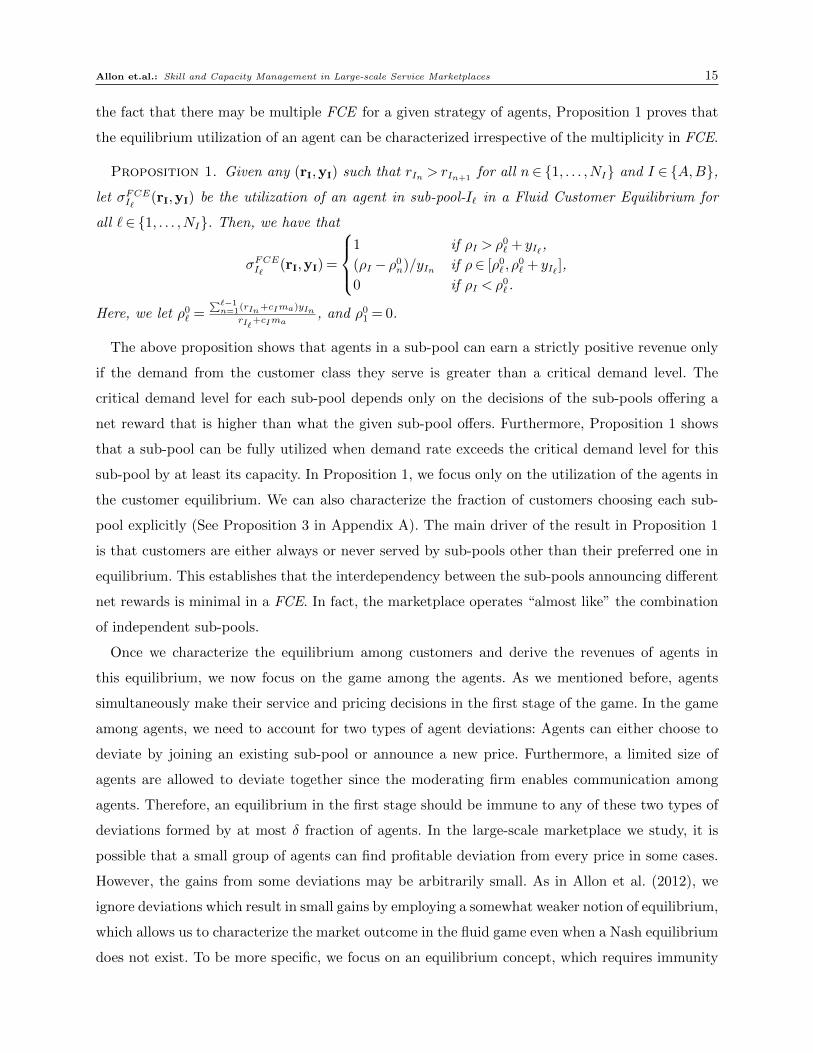
the fact that there may be multiple FCE for a given strategy of agents, Proposition 1 proves that
the equilibrium utilization of an agent can be characterized irrespective of the multiplicity in FCE.
Proposition 1. Given any (rI
,yI
) such that rIn > r
In+1
for all n2 {1, . . . ,NI
} and I 2 {A,B},
let �FCE
I`(r
I
,yI
) be the utilization of an agent in sub-pool-I`
in a Fluid Customer Equilibrium for
all `2 {1, . . . ,NI
}. Then, we have that
�
FCE
I`(r
I
,yI
) =
8
>
<
>
:
1 if ⇢I
> ⇢
0
`
+ y
I`,
(⇢I
� ⇢
0
n
)/yIn if ⇢2 [⇢0
`
,⇢
0
`
+ y
I`],
0 if ⇢I
< ⇢
0
`
.
Here, we let ⇢0`
=P`�1
n=1
(rIn+cIma)yInrI`
+cIma, and ⇢
0
1
= 0.
The above proposition shows that agents in a sub-pool can earn a strictly positive revenue only
if the demand from the customer class they serve is greater than a critical demand level. The
critical demand level for each sub-pool depends only on the decisions of the sub-pools o↵ering a
net reward that is higher than what the given sub-pool o↵ers. Furthermore, Proposition 1 shows
that a sub-pool can be fully utilized when demand rate exceeds the critical demand level for this
sub-pool by at least its capacity. In Proposition 1, we focus only on the utilization of the agents in
the customer equilibrium. We can also characterize the fraction of customers choosing each sub-
pool explicitly (See Proposition 3 in Appendix A). The main driver of the result in Proposition 1
is that customers are either always or never served by sub-pools other than their preferred one in
equilibrium. This establishes that the interdependency between the sub-pools announcing di↵erent
net rewards is minimal in a FCE. In fact, the marketplace operates “almost like” the combination
of independent sub-pools.
Once we characterize the equilibrium among customers and derive the revenues of agents in
this equilibrium, we now focus on the game among the agents. As we mentioned before, agents
simultaneously make their service and pricing decisions in the first stage of the game. In the game
among agents, we need to account for two types of agent deviations: Agents can either choose to
deviate by joining an existing sub-pool or announce a new price. Furthermore, a limited size of
agents are allowed to deviate together since the moderating firm enables communication among
agents. Therefore, an equilibrium in the first stage should be immune to any of these two types of
deviations formed by at most � fraction of agents. In the large-scale marketplace we study, it is
possible that a small group of agents can find profitable deviation from every price in some cases.
However, the gains from some deviations may be arbitrarily small. As in Allon et al. (2012), we
ignore deviations which result in small gains by employing a somewhat weaker notion of equilibrium,
which allows us to characterize the market outcome in the fluid game even when a Nash equilibrium
does not exist. To be more specific, we focus on an equilibrium concept, which requires immunity

16 Allon et.al.: Skill and Capacity Management in Large-scale Service Marketplaces
against only deviations that improve the revenue of an agent by at least ✏> 0 as formally stated
in Definition 2 (see below). We refer to ✏ as the level of equilibrium approximation and suppose
it is arbitrarily close to zero. To ease notation, we denote R
I
(!A
,!
B
) and R
IF
(!A
,!
B
) by R
I
and
R
IF
, respectively, for any given exam threshold pair (!A
,!
B
) and any I 2 {A,B}. We also let
eI
x ⌘ (exIn)NIn=1
denote the N
I
-dimensional vector with a 1 in the x
th coordinate and 0 elsewhere.
Definition 2 (Fluid Market Equilibrium). Let (rI
,yI
) ⌘ (rIn , yIn)
NIn=1
summarize the
strategy of all agents in the marketplace for any I 2 {A,B}. Then, (rI
,yI
) is a (✏, �)-Fluid Market
Equilibrium ((✏, �)-FME) if the following conditions are satisfied.
1. For any `N
I
, mN
I
, 0< dmin{yI`, �}, and I 2 {A,B}, we have that
[RI
� r
`
]�FCE
I`(r
I
,yI
) � [RI
� r
m
]�FCE
Im(r
I
,y0I
)� ✏ (9)
[RIF
� r
`
]�FCE
I`(r
I
,yI
) � [RIF
� r
m
]�FCE
Im(r
I
,y0I
)� ✏, (10)
where y0I
= yI
� deI
` + deI
m.
2. For any `N
I
, 0< dmin{yI`, �}, I 2 {A,B}, and r
0 6= r
In for all nN
I
, we have that
[RI
� r
`
]�FCE
I`(r
I
,yI
) � [RI
� r
0]�FCE
INI+1
(r0I
,y0I
)� ✏, (11)
[RIF
� r
`
]�FCE
I`(r
I
,yI
) � [RIF
� r
0]�FCE
INI+1
(r0I
,y0I
)� ✏, (12)
where r0I
= (rI
, r
0), and y0I
= (yI
, d).
3. For any `N
I
, mN
J
, 0< dmin{yI`, �}, I, J 2 {A,B}, and I 6= J , we have that
[RIF
� r
`
]�FCE
I`(r
I
,yI
) � [RJF
� r
m
]�FCE
Jm(r
J
,y0J
)� ✏, (13)
where y0J
= yJ
+ deJ
m.
4. For any `N
I
, 0< dmin{yI`, �}, I, J 2 {A,B}, I 6= J , r0 6= r
Jn for all n,N
J
, we have that
[RIF
� r
`
]�FCE
I`(r
I
,yI
) � [RIJ
� r
0]�FCE
JNJ+1
(r0J
,y0J
)� ✏, (14)
where r0J
= (rJ
, r
0), and y0J
= (yJ
, d).
Moreover, (rI
,yI
) is a Fluid Market Equilibrium (FME) if there exists a sequence (rI
k
,yI
k) such
that (rI
k
,yI
k) is a (✏k, �k)-FME for any k= 1,2, . . . where ✏
k ! 0, �k ! 0, and (rI
k
,yI
k)! (rI
,yI
)
for all nN
I
as k!1.
(9) and (11) in the (✏, �)-FME definition state that dedicated agents have no incentive to deviate.
Note that dedicated agents cannot change the customer class they serve. Therefore, (✏, �)-FME
accounts for two possible deviations for dedicated agents: joining an existing sub-pool or creating
a new one. On the other hand, flexible agents have the option of changing the customer class they
serve. Thus, (✏, �)-FME ensures that flexible agents cannot improve their revenues whether they
change the customer class they serve or not. In particular, (10) and (12) focus on flexible agent
deviations when they keep the customer class they serve the same, whereas (13) and (14) consider
deviations where flexible agents change the class they serve. Finally, we conclude that a strategy

Allon et.al.: Skill and Capacity Management in Large-scale Service Marketplaces 17
profile is a Fluid Market Equilibrium (FME) if it is the limit of (✏, �)-FME as both ✏ and � becomes
arbitrarily small.
The above definition of the market equilibrium has no restriction on the structure of the emerging
equilibrium outcome. Particularly, we do not rule out an asymmetric equilibrium outcome, where
the same type of agents (dedicated or flexible) charge di↵erent prices to serve the same customer
class. Despite the quite general equilibrium definition, we show that the possibility of asymmetric
equilibrium is very limited. Proposition 2 proves that the same type of agents serving the same
customer class in any asymmetric FME must earn zero revenue. In other words, any asymmetric
FME is outcome-equivalent (from the agents’ point of view) to a symmetric FME where the same
type of agents serving the same customer class charge their operating costs, which is normalized to
zero. It also shows that the equilibrium revenues of flexible agents must be the same regardless of
the customer class they serve. Hence, Proposition 2 establishes that the same type of agents earn
the same revenue in any FME. This nice property of the equilibrium eases our analysis significantly.
Proposition 2. Given any FME (rI
,yI
), let VFME
IDnand V
FME
IFnbe the equilibrium revenue of a
dedicated and a flexible agents in sub-pool-In
for all I 2 {A,B}, respectively.1. If the number of di↵erent prices announced by the dedicated (flexible) agents serving class-I is
two or more for some I 2 {A,B}, then we have that VFME
IDn= 0 (V
FME
IFn= 0) for all n2 {1, . . . ,N
I
}.2. V
FME
AFn= V
FME
BFmfor any n2 {1, . . . ,N
A
}, m2 {1, . . . ,NB
}.
We next start to characterize the equilibrium outcome in a marketplace with a special market
structure, namely one customer class and two types of agents. This structure constitutes the build-
ing block of a marketplace with two classes. Carrying out our analysis in this building block model
is a fundamental step towards finding the equilibrium outcome of the whole marketplace. It also
allows us to discuss the intuition behind our results in a more clear way.
5.1. A Special Marketplace Structure
As we mentioned before, the moderating firm may set up the skill-mix structure in the marketplace
(i.e., the capacity of dedicated and flexible agents) by changing the thresholds levels in each exam.
We illustrate the possible skill-mix structures that can arise after the firm’s choice of exam threshold
pair in Figure 1. We observe that “Inverted V-Network,” where there is only one customer class and
two types of agents, is the key to characterize the equilibrium outcome in any skill-mix structure.
For instance, once the agents make their service decisions in an M-Network, we need to analyze
two separate Inverted V-Networks, in each of which one customer class can be served by both
dedicated and flexible agents. Similarly, we can obtain the equilibrium outcome in other skill-mix
structures by analyzing two separate Inverted V-Networks. Therefore, in this section, we study the
equilibrium outcome of this special market structure, the Inverted V-Network.

18 Allon et.al.: Skill and Capacity Management in Large-scale Service Marketplaces
We consider a marketplace, where there is only one class of customers, but there are two types
of agents, say dedicated and flexible, who can serve these customers. We assume that the arrival
rate of customers is ⇢. As we have two types of agents, we let ↵
D
be the capacity of dedicated
agents, and ↵
F
be the capacity of flexible agents. Furthermore, we assume that customers earn
a reward of RD
when their service is completed by a dedicated agent, and they earn R
F
when a
flexible agent serves them. Finally, we denote the waiting cost by c. We keep all other assumptions
we made in Section 3, and we will use the equilibrium concepts introduced in Section 5. We refer
to the marketplace as buyer’s market if ⇢< ↵
D
+↵
F
and seller’s market otherwise.
As we show in Proposition 2, agents in the same pool (dedicated or flexible) earn zero revenue
in any asymmetric Fluid Market Equilibrium (FME ). In other words, any emerging asymmetric
FME should be outcome-equivalent to a symmetric FME, where agents in the same pool charge
the same price and earn zero revenue in equilibrium. Based on this relationship, our approach
to characterize the equilibrium outcome is as follows: We first derive the equilibrium revenues of
agents in any symmetric FME, where all dedicated agents charge the same price pD
, and all flexible
agents charge p
F
. If there is a symmetric equilibrium where the equilibrium revenue of agents in a
pool (dedicated or flexible) is zero, we can ignore any asymmetric equilibrium where agents in this
pool charge di↵erent prices because such an asymmetric equilibrium will not provide any further
information about the revenues of the agents. Otherwise, we will check if there is any asymmetric
equilibrium, where agents in this pool charge di↵erent prices.
As a first step towards characterizing the symmetric equilibrium, we derive the revenue of agents
when all the agents in the same pool charge the same price as follows:
Corollary 1. Let VFCE
D
(pD
, p
F
) and V
FCE
F
(pD
, p
F
) be the revenue of a dedicated and a flexible
agent, respectively, when all the dedicated agents charge p
D
and all flexible agents charge p
F
. If
R
D
� p
D
6=R
F
� p
F
, then we have that
V
FCE
h
(pD
, p
F
) =
(
p
h
(⇢/↵h
) if ⇢ ↵
h
p
h
if ⇢> ↵
h
,and V
FCE
l
(pD
, p
F
) =
8
>
<
>
:
0 ⇢< ⇢
0
l
p
l
(⇢� ⇢
0
l
)/↵l
⇢2 [⇢0l
,⇢
0
l
+↵
l
]
p
l
⇢> ⇢
0
l
+↵
l
,
where ⇢
0
l
= Rh�ph+cmaRl�pl+cma
↵
h
h= argmaxi2{D,F}(Ri
� p
i
), and l= argmini2{D,F}(Ri
� p
i
).
The above corollary, which follows as an implication of Proposition 1, establishes that the agent
pool o↵ering the higher net reward (dedicated or flexible) will always be “over-utilized” as long
the total demand exceeds their capacity. On the other hand, the pool o↵ering the lower net reward
will be “under-utilized” unless ⇢ is su�ciently high.
Using the above result, the agent pool o↵ering the lower net reward will always be “under-
utilized” in a buyer’s market since we have that ⇢0l
+↵
l
> ↵
D
+↵
F
. In other words, the demand rate,
⇢, cannot be high enough to let the agent pool o↵ering the lower net reward be “over-utilized.” We

Allon et.al.: Skill and Capacity Management in Large-scale Service Marketplaces 19
show that this will create an opportunity for the members of that pool to improve their revenue
by slightly decreasing their price. Hence, in a buyer’s market, we can only have a symmetric
equilibrium where only one of the agent pools (dedicated or flexible) earn positive revenue. In fact,
Theorem 1 below establishes that the pool generating higher customer reward can earn positive
revenue in a buyer’s market once the demand exceeds their capacity.
The above corollary also states that both pools can be over-utilized in a seller’s market. In this
case, cutting the price does not help the agents to improve their revenues. However, we show that
in this setting, a small fraction of agents from the group o↵ering the higher net reward will have
an opportunity to increase their prices and improve their revenues. Thus, in a seller’s market, all
agents, regardless of their group, o↵er the same net reward in a symmetric equilibrium. We formally
present these observations in the following result:
Theorem 1. Let VFME
D
and V
FME
F
be the revenue of a dedicated and a flexible agent, respec-
tively, in a FME of a marketplace with one customer class and two agent pool. Then, letting
h= argmaxi2{D,F}
R
i
, and l= argmini2{D,F}
R
i
, we have that:
1. If ⇢< ↵
h
, then we have that VFME
h
= V
FME
l
= 0.
2. If ⇢= ↵
h
, then we have that VFME
h
R
h
�R
l
, and V
FME
l
= 0.
3. If ↵h
< ⇢< ↵
h
+↵
l
, then we have that VFME
h
=R
h
�R
l
, and V
FME
l
= 0.
4. If ⇢= ↵
h
+↵
l
, then we have that VFME
h
= V
FME
l
+(Rh
�R
l
), and V
FME
l
R
l
.
5. If ⇢> ↵
h
+↵
l
, then we have that VFME
h
=R
h
, and V
FME
l
=R
l
.
When we focus on the case where customers earn more reward from the dedicated agents (which
reduces to the setting h=D and l= F in Theorem 1), the above theorem shows that the dedicated
agents can only charge their operating costs in a symmetric equilibrium when demand is low, and
in such a setting, only the dedicated agents can serve customers. Thus, all agents earn zero in
equilibrium when demand is low in a buyer’s market. Once the demand rate exceeds the capacity
of dedicated agents, ↵D
, the revenues of the dedicated agents in a buyer’s market can be positive,
yet below R
D
� R
F
, the di↵erence between the customers rewards generated by di↵erent types
of agents. When demand is equal to ↵
D
, there are multiple equilibria and dedicated agents may
charge any price less than or equal to R
D
�R
F
in equilibrium. However, they can agree on charging
R
D
�R
F
in equilibrium when demand rate is strictly greater than their capacity. Dedicated agents
are fully utilized in such an equilibrium and thus earn R
D
�R
F
. The intuition behind this result is
the following: The rate of customers requesting service from the dedicated agents will exceed their
processing capacity when dedicated agents charge a price lower than R
D
�R
F
. Therefore, customers
experience significant waiting times and incur a strictly positive waiting cost. Using the fact that
customers pay an extra cost, a small group of agents can increase their prices while ensuring that
20 Allon et.al.: Skill and Capacity Management in Large-scale Service Marketplaces
they are still over-utilized after the price increase. Since this small group of agents increases their
prices without hurting their utilization, this deviation clearly improves their revenues.
Theorem 1 also shows that flexible agents can earn a strictly positive revenue only in a seller’s
market. When the demand rate is equal to the total processing capacity, there are multiple equilibria
and the equilibrium revenue of flexible agents can be any value below R
F
. However, once the
demand rate is strictly greater than the total service capacity, revenues of both dedicated and
flexible agents must be equal to the customer reward they generate in a symmetric equilibrium. In
such an equilibrium, agents charge their highest prices, and the rate of customers requesting service
is equal to the total capacity, ↵D
+ ↵
F
. In other words, the equilibrium behavior of the agents
avoids any congestion in the system while extracting all of the customer surplus. The main driver
of this result is similar to the intuition given above: There is congestion in the system when all
agents earn less than the reward they generate, and this creates an incentive for agents to increase
their prices. Once we obtain the revenues of agents in any symmetric equilibrium, we now discuss
asymmetric equilibria. As we mentioned before, we only need to pay attention to asymmetric
equilibria when agents in a pool earn strictly positive revenues in any symmetric equilibrium. In
the proof of Theorem 1, we show that an asymmetric FME cannot emerge in such a circumstance.
Particularly, we rule out the possibility of asymmetric equilibrium, where the dedicated agents
charge di↵erent prices, for any demand rate ⇢ > ↵
D
. Similarly, there cannot be any asymmetric
equilibrium, where the flexible agents charge di↵erent prices, when ⇢> ↵
D
+↵
F
.
After characterizing the equilibrium outcome in our building-block model, we next turn our
attention to the moderating firm’s skill-mix and capacity decisions.
Remark 1. The marketplace we consider in this section is similar to the one with noniden-
tical agents studied in Allon et al. (2012). Allon et al. (2012) develops an asymptotic theory to
understand the behavior of the equilibrium along the sequence of marketplaces growing in size.
The methodology developed in Allon et al. (2012) can easily become analytically intractable while
analyzing more complex problems such as the moderating firm’s skill and capacity management
problem. Thus in this paper, we focus directly on the limiting game, whose results are easy to incor-
porate into the moderating firm’s problem while capturing the main managerial insights obtained
from an asymptotic analysis. Furthermore, given that we use a fluid model in the limiting game,
we also investigate the outcomes of asymmetric equilibria, which are ignored in Allon et al. (2012).
6. The Skill-Mix and Capacity Management of the Moderating Firm
As we mentioned in the Introduction, the profit of the moderating firm is a share of the total revenue
generated in the marketplace. Therefore, in order to maximize its profit, the firm has to maximize
the total revenue in the marketplace by choosing the appropriate exam threshold pair (!A
,!
B
).

Allon et.al.: Skill and Capacity Management in Large-scale Service Marketplaces 21
Once the firm chooses the exam thresholds, a Fluid Market Equilibrium will emerge, and using
the outcome of this equilibrium one can calculate the revenue generated in the marketplace. We
denote the total revenue in the marketplace by ⇧(!A
,!
B
) given any exam threshold pair (!A
,!
B
).
Notice that while Theorem 1 shows that there might be multiple equilibria, this multiplicity
happens only if a given exam threshold pair (!A
,!
B
) leads to a knife-edge case, i.e., the demand
rate of a class is equal to the capacity of the dedicated and/or the flexible agents serving this
class. For mathematical convenience, we will be focusing on the equilibrium generating the highest
possible revenue among all possible equilibria1. We let V
F
(!A
,!
B
) be the highest equilibrium
revenue of a flexible agent, and V
ID
(!A
,!
B
) be the highest equilibrium revenue of a dedicated
agent serving class-I for all I 2 {A,B}2. Then, we write the total revenue in the marketplace as
⇧(!A
,!
B
) =P
I2{A,B}�
V
ID
(!A
,!
B
)↵I
(!A
,!
B
)�
+V
F
(!A
,!
B
)↵F
(!A
,!
B
).
We need to characterize the profit function ⇧(!A
,!
B
) for any given exam threshold pair (!A
,!
B
)
to find the optimal skill-mix and capacity decision of the moderating firm. Based on our results
in Theorem 1, we know that the equilibrium revenue of an agent can change significantly even
after the firm slightly modifies the exam thresholds in a marketplace. For instance, the revenue
of an agent may go down from his highest price to zero when the moderating firm increases the
service capacity available to the customer class he is serving by a small amount. Therefore, the
firm’s profit function has di↵erent functional forms in di↵erent regions of exam threshold space
[0, RA
]⇥ [0, RB
]. Finding the optimal exam threshold pair requires comparing all these di↵erent
functional forms, which is analytically intractable when the skills of an agent, SA
and S
B
, follow
a general joint probability distribution. To have a tractable problem, in this section, we study the
skill-mix and capacity decision of the firm by imposing three di↵erent conditions on S
A
and S
B
:
1. S
A
and S
B
are perfectly positively correlated: P ({SA
= S
B
}) = 1,
2. S
A
and S
B
are perfectly negatively correlated: P ({SA
+S
B
= 1}) = 1,
3. S
A
and S
B
are independent and identically distributed.
We also restrict our attention to a seller’s market, where the total demand rate exceeds the total
service capacity of candidate agents. We provide a brief discussion on the firm’s optimal decisions
when this assumption is relaxed.
1 When there are multiple equilibria in a marketplace, the moderating firm can sustain the equilibrium with thehighest revenue by perturbing the thresholds levels (!A,!B) slightly. For instance, if the marketplace were in a knife-edge case described in Theorem 1.4, the firm could increase the exam threshold by an arbitrarily small amount andmove the marketplace to the case described in Theorem 1.5. Such a change would make sure that there is a uniqueequilibrium and the total revenue in the marketplace is arbitrarily close to the highest level among the multipleequilibria before the change.
2 Proposition 2 shows that the same type of agents (dedicate or flexible) must earn the same revenue for any givenequilibrium even if they charge di↵erent prices. Therefore, we can denote the revenues of the same type of agents inany given equilibrium by a unique value.

22 Allon et.al.: Skill and Capacity Management in Large-scale Service Marketplaces
6.1. Positively Correlated Skills
We start with studying the skill-mix and capacity decision of the firm in a marketplace where
S
A
= S
B
and S
A
is random with continuous distribution F (·) on the support [0,1]. We denote
the mean of SA
by µ. Given this structure, we can derive the capacity of dedicated and flexible
agents for any pair of thresholds (!A
,!
B
) using (1). Similarly, the reward that a customer expects
from a certain pool of agents can be calculated using (2)-(3). As we have S
A
= S
B
, the expected
reward from flexible agents is the same for both classes of customers, and thus will be denoted by
R
F
(!A
,!
B
) in this subsection.
When the skills of an agent are positively correlated, the moderating firm can create three
di↵erent skill-mix structures: a) one with only flexible agents, the so-called V-Network, (by set-
ting !
A
= !
B
), b) one with flexible agents and dedicated agents only for class-A, the so-called
N-Network, (by setting !
A
> !
B
), c) one with flexible agents and dedicated agents only for class-B
(by setting !
A
< !
B
). In a marketplace with only flexible agents, agents can extract all of the
customer surplus as discussed in Theorem 1 since the total demand rate is higher than poten-
tial service capacity, i.e., ⇢A
+ ⇢
B
� 1. Therefore, the total revenue generated in a V -Network is
R
F
(!A
,!
B
)↵F
(!A
,!
B
). On the other hand, agents may not extract all of the customer surplus in
an N -Network because they may not charge the highest price that they can charge in equilibrium.
In fact, we show that even if they extract all of the customer surplus, the total revenue generated in
a marketplace with dedicated agents cannot exceed the revenue in a marketplace with only flexible
agents keeping the capacity of eligible agents constant. Thus, keeping the total service capacity
constant, the moderating firm is (weakly) better o↵ having only flexible agents.
Once we establish that the firm prefers V -Network over N -Network, it is su�cient to focus on
the firm’s profit on skill-mix structures with only flexible agents. When there are only flexible
agents in the marketplace, i.e., !A
= !
B
= ! for some ! 2 [0,1], the total service capacity, ↵F
(!,!),
decreases in ! whereas higher threshold levels lead to higher expected reward, RF
(!,!). Thus,
the firm has to trade-o↵ between the total service capacity and the equilibrium revenue of agents.
It turns out, the firm strictly prefers higher capacity since R
F
(!,!)↵F
(!,!), which is equal toR
1
!
sf(s), is decreasing in !. This implies that the moderating firm always chooses to use all of its
available service capacity. Specifically, it sets the exam threshold pair to (0,0), i.e., all agents pass
both exams. The following theorem formally presents these results.
Theorem 2. When S
A
= S
B
and S
A
is random with continuous distribution F (n) on support
[0,1], we have that
1. ↵
A
(!⇤A
,!
⇤B
) + ↵
F
(!⇤A
,!
⇤B
) + ↵
B
(!⇤A
,!
⇤B
) = 1 for any threshold levels (!⇤A
,!
⇤B
) that maximize
the total revenue in the marketplace.
2. The exam threshold pair (0,0) maximizes the total revenue in the marketplace.
Allon et.al.: Skill and Capacity Management in Large-scale Service Marketplaces 23
6.2. Negatively Correlated Skills
After studying the positively correlated skills, we now characterize the optimal skill-mix and capac-
ity decision of the moderating firm in a setting where SA
+S
B
= 1 and S
A
is random with continuous
distribution F (·) on support [0,1]. We denote the mean of SA
by µ. For any given pair of threshold
levels (!A
,!
B
), the capacity of each agent pool and the reward that a customer expects from a
certain pool can be calculated using (1)-(3).
In a marketplace where an agent’s skills are negatively correlated, there are two di↵erent skill-mix
structures that can arise: a) one with only dedicated agents for each class, the so-called I-Network,
(by setting !
A
+ !
B
� 1), and b) one with flexible agents and dedicated agents for each class,
the so-called M-Network, (by setting !
A
+!
B
< 1). In a marketplace with only dedicated agents,
there is a separate marketplace for each customer class. Then, by Theorem 1, the equilibrium
revenue of an agent serving class-I is the expected reward his pool generates, RI
(!A
,!
B
), if the
marketplace for class-I is a seller’s market, i.e., ↵I
(!A
,!
B
) ⇢
I
, and zero otherwise for all I 2{A,B}. Therefore, the firm never creates a marketplace where the service capacity of a dedicated
pool exceeds its demand. Furthermore, the revenue generated in each separate seller’s market
increases by its service capacity, as we discuss in Section 6.1. Thus, the moderating firm always
prefers to increase the service capacity in each separate marketplace while making sure that the
dedicated capacity for each customer class is less than their demand. In fact, among all exam
threshold pairs resulting in a skill-mix structure with only dedicated agents, the firm prefers the
ones which use all candidate agents and create two separate seller’s markets, i.e. any (!A
,!
B
) with
!
A
+ !
B
= 1 and F
�1(1� ⇢
A
) !
A
F
�1(⇢B
). Note that the firm uses all of its available service
capacity for any exam threshold pair resulting in a marketplace with both flexible and dedicated
agents. Therefore, the moderating firm always uses all of its available service capacity to maximize
its profits as in the case of positively correlated skills. This finding is summarized in Theorem 3.1.
We also show that the revenue generated in a marketplace with both flexible and dedicated agents
cannot exceed the revenue in a marketplace where the firm utilizes all candidate agents and creates
two separate seller’s markets. Hence, in a marketplace with negatively correlated agent skills, the
moderating firm can maximize its profits by creating two separate seller’s markets and using all of
its available service capacity.
After showing that creating two separate seller’s market maximizes the profits of the firm, the
question that still remains is how the firm divides the service capacity between these two market-
places. As the firm prefers to use all of its available service capacity, an increase in the capacity
allocated to one class decreases the capacity for the other one. Since more capacity means higher
revenue in a seller’s market, the moderating firm trades-o↵ between the gains from increasing the
capacity for one class and the losses from decreasing the capacity for the other one. Also, note

24 Allon et.al.: Skill and Capacity Management in Large-scale Service Marketplaces
that some of the customers from a class do not request service when the capacity allocated to this
class is strictly less than its demand rate as discussed before in Theorem 1. Therefore, the service
capacity allocated to a class should not be less than its demand rate if the firm wants to serve
all customers from this class. We say the firm favors a class when it allocates enough capacity to
serve all customers from this class.
It turns out that the gains from increasing the service capacity for class-A dominate the firm’s
losses in the marketplace for class-B when the demand from class-A is lower than a critical demand
level, which is 1 � F (1/2). Thus, if ⇢A
< 1 � F (1/2), the moderating firm increases the service
capacity for class-A until the capacity equals the demand from this class and allocates the rest of
the agents to class-B. As a result of this skill-mix structure, all of the class-A customers obtain
service whereas some of the class-B customers do not request service since the demand from class-
B is more than the service capacity allocated to this class. In other words, the moderating firm
favors class-A when ⇢
A
< 1�F (1/2). Similarly, the firm maximizes its profits by favoring class-B
when the demand from class-B is lower than the critical demand level of F (1/2). As a customer
class is favored when its demand rate is lower than a critical level, the firm favors a class if its
demand rate is too low. The driver of this result is the fact that only the agents generating very
high customer rewards can serve the class with too low demand even if all of the customers from
this class are served. Then, one may expect that the firm always favors the customer class with
lower demand rate because the expected reward of the customers from this class is always higher
but this intuition is not true. For instance, when F (1/2)< 1/2, the firm may favor class-A even
if ⇢A
> ⇢
B
. This, actually, proves the significance of the skill distribution function in the firm’s
skill-mix and capacity allocation problem.
It is also possible that the demand from both classes exceed the corresponding demand thresholds
discussed above. In such a case, the moderating firm maximizes its profits at a pair of threshold
levels where the marginal gains from increasing the service capacity for one class is equal to the
marginal loss from decreasing the capacity for the other class. This happens when the firm allocates
F (1/2) fractions of agents to class-B and the rest to class-A. Under such a screening mechanism,
the firm rejects customers from both classes.
Besides the optimal exam threshold pair that creates a marketplace with only dedicated agents,
the firm may maximize its profits by using exam threshold pairs which lead to a marketplace with
flexible agents. We show that the flexible agents prefer to serve the same customer class when the
firm uses such an optimal exam threshold pair. Therefore, even though there are flexible agents in
the marketplaces, the firm ensures that they behave as if they are dedicated agents to maximize its
profits. Furthermore, the firm allocates enough capacity to serve all customers from class-A when
⇢
A
< 1� F (µ) and class-B when ⇢
B
< F (µ) under any optimal pair of exam thresholds allowing
for flexible agents. We formally present the above results in Theorem 3.

Allon et.al.: Skill and Capacity Management in Large-scale Service Marketplaces 25
Theorem 3. When S
A
+S
B
= 1 and S
A
is random with continuous distribution F (n) on support
[0,1], we have that
1. ↵
A
(!⇤A
,!
⇤B
) + ↵
F
(!⇤A
,!
⇤B
) + ↵
B
(!⇤A
,!
⇤B
) = 1 for any threshold levels (!⇤A
,!
⇤B
) that maximize
the total revenue in the marketplace.
2. The threshold levels (!⇤,1�!
⇤) maximize the total revenue in the marketplace, where
!
⇤ =
8
<
:
F�1(1� ⇢A) if F�1(1� ⇢A)> 1/2
1/2 if F�1(1� ⇢A) 1/2 F�1(⇢B)
F�1(⇢B) if F�1(⇢B)< 1/2.
3. If ↵
F
(!⇤A
,!
⇤B
) > 0 for a pair of threshold levels (!⇤A
,!
⇤B
) that maximize the total revenue
in the marketplace, then all of flexible agents serve the same customer class in the equilibrium.
Furthermore, the firm favors class-A when ⇢
A
< 1�F (1/2) and class-B when ⇢
B
<F (1/2).
Up to here, we have considered the firm’s skill-mix and capacity decisions when the skills of each
agent are perfectly correlated. We, now, turn to discuss marketplaces where an agent’s skills are
independent.
6.3. Independent Skills
In the previous subsections, we focus on marketplaces where an agent’s skills are perfectly corre-
lated. Now, we study the moderating firm’s problem in a setting where the skills of an agent are
independent and identically distributed. Particularly, we assume that both S
A
and S
B
are random
with continuous distribution F (·) on the support [0,1]. We denote the mean of SA
and S
B
by µ.
As in the previous cases, we can derive the capacity of each agent pool and the reward that a
customer expects from a certain pool using (1)-(3) for any given exam threshold pair (!A
,!
B
).
Recall from Sections 6.1 and 6.2 that at the optimal skill-mix structure, the moderating firm
utilizes all of its available capacity when agent skills are perfectly correlated in a seller’s market.
This is somewhat expected given the fact that total demand exceeds the available service capacity.
The main driver of this result is that the moderating firm has no incentive to reduce the service
capacity allocated to one customer class while keeping the capacity allocated for the other one
unchanged. However, we show that the firm may benefit from limiting the capacity allocated to
one class while keeping the capacity for the other class constant in a marketplace where an agent’s
skills are independent. This can be graphically illustrated by using Curve A and B in Figure 3.
For any threshold pair (!A
,!
B
) on Curve A, we have that (i) the skill-mix structure is an M -
Network with dedicated agents for each class and flexible agents, (ii) the capacity of dedicated
agents for class-A is constant and equal to the demand rate of class-A, ⇢A
, (iii) all flexible agents
choose to serve class-B in equilibrium, and (iv) all agents charge the highest price they can charge.
As the firm moves on Curve A in the direction pointed by arrows (which could be achieved by
increasing both of the exam thresholds), it faces a trade-o↵: The profit from class-A increases

26 Allon et.al.: Skill and Capacity Management in Large-scale Service Marketplaces
-!A
6!B
1
1
F
-1(⇢A)
-
Curve A: Any (!A
,!
B
)with F (!
A
) = 1� ⇢AF (!B)
F
-1(⇢B)
-
Curve B: Any (!A
,!
B
)with F (!
B
) = 1� ⇢BF (!A)
Figure 3 Curve A (B): Threshold pairs (!A,!B) where the capacity of dedicated agents for class-A (class-B) is
equal to the demand rate of class-A (class-B), ⇢A (⇢B).
because the average skill of a dedicated agent serving class-A increases whereas the profit from
class-B decreases because the service capacity allocated to this class decreases. When the demand
from class-A is less than the critical demand level of F (µ), we show that the gains from class-A
outweighs the losses from class-B on Curve A for exam threshold pairs with zero or low thresholds
in Exam-A. Thus, the firm is better o↵ increasing the threshold levels rather than letting all agents
pass Exam-A, which implies that there is an interior exam threshold pair that maximizes firm’s
profit on Curve A. We also show that this interior threshold pair generates more profit than any
exam threshold pairs allowing all candidate agents to pass Exam-A, i.e., exam threshold pairs with
!
A
= 0. Similarly, the firm does not allow all candidate agents to pass Exam-B when the demand
from class-B is less than F (µ). Hence, when both demand rates are less than F (µ), it is not optimal
to allow all candidate agents in the marketplace to serve customers. In other words, the firm has
to fail some of the candidate agents in both exams in order to maximize the revenue generated
in a marketplace where agent skills are independent when both demand rates are lower than the
critical demand level of F (µ).
Having both demand rates less than F (µ) is possible only if the mean of the skill distribution
is greater than its median, i.e. F (µ)� 1/2. If F (µ) is less than 1/2, the higher of the two demand
rates is greater than the threshold F (µ) since we consider a seller’s market with ⇢
A
+ ⇢
B
> 1. We
assume the higher demand rate corresponds to ⇢
A
for ease of explanation. As ⇢A
>F (µ), the firm’s
gains fall short of its losses when the firm increases the exam thresholds on Curve A, and thus the
threshold pair (0, F�1(⇢A
)) maximizes firm’s profit on Curve A. On the other hand, the demand
rate of class-B can still be less than F (µ). If the demand rate of class-B is less than F (µ), the
firm will be better o↵ choosing an interior point on Curve B rather than allowing all agents to

Allon et.al.: Skill and Capacity Management in Large-scale Service Marketplaces 27
pass Exam-B. Thus, the firm compares its profits under two exam threshold pairs: one lets all
candidate agents pass Exam-A whereas the other one fails some of the candidate agents in both
exams. We show that if the skill distribution function F (·) is convex3, the firm’s profits from the
threshold pair failing agents outweigh its profits from the one letting all agents serve customers4.
Hence, even if the mean of the skill distribution is less than its median, the optimal exam threshold
pair prescribes to limit service capacity in a seller’s market. We formally present these results in
the following theorem.
Theorem 4. When S
I
is random with continuous distribution F (·) on support [0,1] for all
I 2 {A,B} and ⇢
A
� ⇢
B
, we obtain the following:
1. If ⇢
A
< F (µ), then we have that ↵A(!⇤A,!
⇤B) + ↵F (!⇤
A,!⇤B) + ↵B(!⇤
A,!⇤B) < 1 for any threshold
levels (!⇤A
,!
⇤B
) that maximize the total revenue in the marketplace. Furthermore, the threshold level⇣
F
�1
⇣
1� ⇢AF (!(⇢A))
⌘
, !(⇢A)⌘
maximizes the total revenue in the marketplace.
2. If ⇢B
< F (µ) and F (·) is convex, then we have that ↵A(!⇤A,!
⇤B) + ↵F (!⇤
A,!⇤B) + ↵B(!⇤
A,!⇤B)< 1
for any threshold levels (!⇤A
,!
⇤B
) that maximize the total revenue in the marketplace. Furthermore,
the threshold level⇣
!
⇤, F
�1
⇣
1� ⇢BF (!⇤
)
⌘⌘
maximizes the total revenue in the marketplace, where
!
⇤ =min{!, !(⇢B
)}.
Here, !(⇢) is the unique solution to1
R
F�1(1� ⇢F (!) )[1 � F (s)]ds = ! for any ⇢ < F (µ), ! = min{! : F (!)[1 �
F (!)] = ⇢B} when ⇢
B
< 1/4, and != 1 when ⇢
B
� 1/4.
Besides the conditions under which the firm fails some of the candidate agents in a seller’s
market, the above theorem also describes the optimal skill-mix decision under these conditions.
The first claim of Theorem 4 shows that the exam threshold pair that maximizes firm’s profit on
Curve A is, in fact, the optimal skill-mix decision among all exam threshold pairs. At this optimal
exam threshold pair, the marginal gain from increasing the expected reward for class-A (while
keeping the capacity of their dedicated agents at ⇢A
) is equal to the marginal loss from reducing the
available capacity for class-B. Since the optimal exam threshold pair in on Curve A, the optimal
skill-mix structure is an M -Network with dedicated agents for each class and flexible agents. The
optimal capacity of dedicated agents serving class-A is equal to the demand from this class. In
the Fluid Market Equilibrium emerging at the optimal skill-mix structure, all agents charge the
highest price that they can charge, and all flexible agents serve class-B.
3 Note that convex F (·) implies that F (µ) 1/2 (See Proposition 3 in Caplin and Nalebu↵ (1991)).
4 To prove this result, we actually need to have that f(F�1(s)) f(F�1(1� s)) for any s 1/2, which is a weakercondition than convex F (·). It is shown that this condition holds for any Beta distribution with shape parameters ↵
and � (i.e., f(s) = s↵�1(1�s)��1
B(↵,�) ) as long as ↵� � � 1 (See Runnenburg (1978) and Zwet (1979)). For simplicity ofour expressions, we do not state our results using this condition.

28 Allon et.al.: Skill and Capacity Management in Large-scale Service Marketplaces
-!A
6!B
1
1F
-1(⇢B)
-Curve B: Any (!
A
,!
B
)with F (!
B
) = 1� ⇢BF (!A)
Figure 4 Threshold pairs (!A,!B) where the capacity of dedicated agents for class-B is equal to the demand
rate of class-B, ⇢B.
The second claim of the above theorem, similar to the first one, establishes that the firm maxi-
mizes its profits by choosing an exam threshold on Curve B when F (·) is convex and ⇢
B
<F (µ).
The optimal skill-mix structure is also an M -Network, and the optimal capacity of dedicated agents
serving class-B is ⇢B
. Moreover, all agents charge the highest price that they can charge. However,
in contrast to the first claim of Theorem 4, it is possible that the marginal gain from increasing
the expected reward for class-B exceeds the marginal loss from reducing the capacity of flexible
agents. This means that the firm would benefit from an increase in both exam thresholds. However,
the firm cannot improve its profits by failing more agents because such a change would cause a
significant shift in the equilibrium behavior of the agents, namely, some of the agents would not
charge their highest price. This can happen when the demand rate of class-B is less than 1/4. If
⇢
B
< 1/4, Curve B intersects with the 45o-line as in Figure 4. At any exam threshold pair on Curve
B and above the 45o-line, dedicated agents serving class-B charge strictly lower than the highest
price they can charge.
Note that unlike the first part of Theorem 4, where it is required to have both demand rates
lower than a critical level, the condition in the second claim of Theorem 4 requires only the demand
rate of class-B to be less than a critical level. Therefore, it may be optimal for the firm to fail
candidate agents even when the demand from class-A is very high.
We performed a numerical study to gain further insight about the firm’s optimal decisions.
We present the optimal skill-mix decision in terms of the percentage of pass and fail in each
exam in Table 1. In our numerical study, we observe that the firm may utilize 93% of the total
service capacity even though the demand from class-A solely exceeds the total available capacity.
Furthermore, the fraction of candidate agents passing a particular exam can be as low as 50%
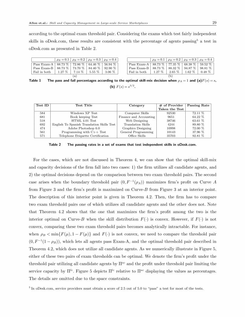
Allon et.al.: Skill and Capacity Management in Large-scale Service Marketplaces 29
according to the optimal exam threshold pair. Considering the exams which test fairly independent
skills in oDesk.com, these results are consistent with the percentage of agents passing5 a test in
oDesk.com as presented in Table 2.
⇢B = 0.1 ⇢B = 0.2 ⇢B = 0.3 ⇢B = 0.4
Pass Exam-A 88.73 % 72.86 % 64.46 % 56.94 %Pass Exam-B 88.73 % 73.70 % 84.40 % 92.90 %Fail in both 1.27 % 7.14 % 5.55 % 3.06 %
(a)
⇢B = 0.1 ⇢B = 0.2 ⇢B = 0.3 ⇢B = 0.4
Pass Exam-A 88.73 % 77.35 % 68.38 % 59.52 %Pass Exam-B 88.73 % 88.32 % 94.87 % 98.81 %Fail in both 1.27 % 2.65 % 1.62 % 0.48 %
(b)
Table 1 The pass and fail percentages according to the optimal skill-mix decision when ⇢A = 1 and (a)F (s) = s,
(b) F (s) = s3/2.
Test ID Test Title Category # of Provider Passing Rate
Taken the Test
584 Windows XP Test Computer Skills 92530 72.11 %681 Book keeping Test Finance and Accounting 9651 64.22 %518 HTML 4.01 Test Web Designing 38746 63.61 %692 English To Spanish Translation Skills Test Translation Skills 4244 89.80 %474 Adobe Photoshop 6.0 Graphics Designing 10998 72.00 %561 Programming with C++ Test General Programming 10143 37.96 %571 Telephone Etiquette Certification O�ce Skills 35703 92.81 %
Table 2 The passing rates in a set of exams that test independent skills in oDesk.com.
For the cases, which are not discussed in Theorem 4, we can show that the optimal skill-mix
and capacity decisions of the firm fall into two cases: 1) the firm utilizes all candidate agents, and
2) the optimal decisions depend on the comparison between two exam threshold pairs. The second
case arises when the boundary threshold pair (0, F�1(⇢A
)) maximizes firm’s profit on Curve A
from Figure 3 and the firm’s profit is maximized on Curve-B from Figure 3 at an interior point.
The description of this interior point is given in Theorem 4.2. Then, the firm has to compare
two exam threshold pairs one of which utilizes all candidate agents and the other does not. Note
that Theorem 4.2 shows that the one that maximizes the firm’s profit among the two is the
interior optimal on Curve-B when the skill distribution F (·) is convex. However, if F (·) is not
convex, comparing these two exam threshold pairs becomes analytically intractable. For instance,
when ⇢
B
<min{F (µ),1� F (µ)} and F (·) is not convex, we need to compare the threshold pair
(0, F�1(1� ⇢
B
)), which lets all agents pass Exam-A, and the optimal threshold pair described in
Theorem 4.2, which does not utilize all candidate agents. As we numerically illustrate in Figure 5,
either of these two pairs of exam thresholds can be optimal. We denote the firm’s profit under the
threshold pair utilizing all candidate agents by ⇧ac and the profit under threshold pair limiting the
service capacity by ⇧lc. Figure 5 depicts ⇧lc relative to ⇧ac displaying the values as percentages.
The details are omitted due to the space constraints.
5 In oDesk.com, service providers must obtain a score of 2.5 out of 5.0 to “pass” a test for most of the tests.

30 Allon et.al.: Skill and Capacity Management in Large-scale Service Marketplaces
0 0.05 0.1 0.15 0.2 0.25 0.3 0.35 0.4−3.5
−3
−2.5
−2
−1.5
−1
−0.5
0
0.5
1
Use allagents
Lim
itserviceca
pacity
Use allagents
(a)
⇧
lc�⇧
ac
⇧
ac
⇢B0 0.05 0.1 0.15 0.2 0.25 0.3 0.35 0.4
−1
−0.5
0
0.5
1
1.5
2
2.5
3
Use allagents
Limitservice capacity
(b)
⇧
lc�⇧
ac
⇧
ac
⇢B
Figure 5 The firm’s profit under the threshold pair described in Theorem 4.2 relative to its profit under the
threshold pair (0, F�1(1� ⇢B)) when ⇢A = 1, (a) SA ⇠Beta(0.5,0.8) and (b) SA ⇠Beta(0.5,0.6).
7. Conclusion
In this paper, we study a marketplace in which many small service providers, who are distinguished
with respect to their service skills, compete with each other in providing service to two groups of
self-interested customers, each of which has di↵erent needs. An important aspect of these mar-
ketplaces that our model captures is that customers cannot learn the skills of a provider before
the completion of the service. However, the moderating firm, which sets up the marketplace, may
help customers by providing them with further information about the ability of candidate agents
through a skill screening mechanism. Such a screening mechanism consists of skill tests determin-
ing whether a candidate agent is eligible to serve customers and helps the firm to create di↵erent
skill-mix structures in the marketplace. The main focus of this paper is on how the moderating firm
uses the skill tests while making skill and capacity management decisions. To this end, we explore
the optimal skill-mix and capacity decisions of the firm by considering three di↵erent structures
for the correlation between the skills of an agent.
The firm faces a natural trade-o↵ while setting up the skill tests: As the tests become more
comprehensive, agents who pass the exams generate more value whereas the marketplace has less
eligible agents. It turns out the firm is better o↵ increasing the eligible service capacity when it
focuses on the profits from only one customer class. This implies that the firm has an incentive
to utilize all candidate agents if it can isolate its business with one class from the other one. We
show that such an isolation is possible when an agent’s skills are perfectly correlated, and thus
the optimal skill-mix and capacity decision of the firm utilizes all candidate agents. On the other
hand, the firm’s profit from one class depends highly on the capacity allocated to the other class
when agent skills are independent. As a result of this interdependence, we show that the firm
benefits from limiting the capacity allocated to one class while keeping the capacity for the other
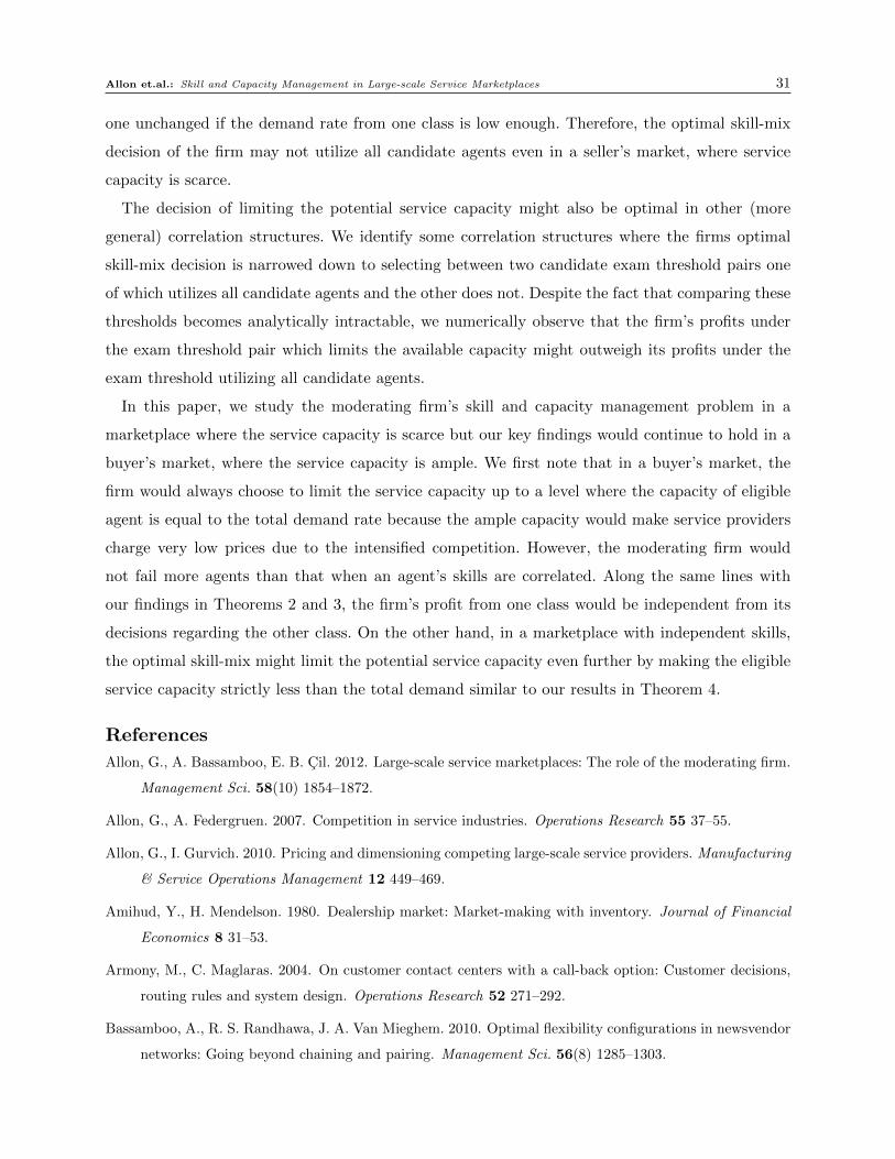
Allon et.al.: Skill and Capacity Management in Large-scale Service Marketplaces 31
one unchanged if the demand rate from one class is low enough. Therefore, the optimal skill-mix
decision of the firm may not utilize all candidate agents even in a seller’s market, where service
capacity is scarce.
The decision of limiting the potential service capacity might also be optimal in other (more
general) correlation structures. We identify some correlation structures where the firms optimal
skill-mix decision is narrowed down to selecting between two candidate exam threshold pairs one
of which utilizes all candidate agents and the other does not. Despite the fact that comparing these
thresholds becomes analytically intractable, we numerically observe that the firm’s profits under
the exam threshold pair which limits the available capacity might outweigh its profits under the
exam threshold utilizing all candidate agents.
In this paper, we study the moderating firm’s skill and capacity management problem in a
marketplace where the service capacity is scarce but our key findings would continue to hold in a
buyer’s market, where the service capacity is ample. We first note that in a buyer’s market, the
firm would always choose to limit the service capacity up to a level where the capacity of eligible
agent is equal to the total demand rate because the ample capacity would make service providers
charge very low prices due to the intensified competition. However, the moderating firm would
not fail more agents than that when an agent’s skills are correlated. Along the same lines with
our findings in Theorems 2 and 3, the firm’s profit from one class would be independent from its
decisions regarding the other class. On the other hand, in a marketplace with independent skills,
the optimal skill-mix might limit the potential service capacity even further by making the eligible
service capacity strictly less than the total demand similar to our results in Theorem 4.
References
Allon, G., A. Bassamboo, E. B. Cil. 2012. Large-scale service marketplaces: The role of the moderating firm.
Management Sci. 58(10) 1854–1872.
Allon, G., A. Federgruen. 2007. Competition in service industries. Operations Research 55 37–55.
Allon, G., I. Gurvich. 2010. Pricing and dimensioning competing large-scale service providers. Manufacturing
& Service Operations Management 12 449–469.
Amihud, Y., H. Mendelson. 1980. Dealership market: Market-making with inventory. Journal of Financial
Economics 8 31–53.
Armony, M., C. Maglaras. 2004. On customer contact centers with a call-back option: Customer decisions,
routing rules and system design. Operations Research 52 271–292.
Bassamboo, A., R. S. Randhawa, J. A. Van Mieghem. 2010. Optimal flexibility configurations in newsvendor
networks: Going beyond chaining and pairing. Management Sci. 56(8) 1285–1303.

32 Allon et.al.: Skill and Capacity Management in Large-scale Service Marketplaces
Biais, B., L. Glosten, C. Spattt. 2005. Market microstructure: A survey of microfoundations, empirical
results, and policy implications. Journal of Financial Markets 8 217–264.
Bish, E. K., Q. Wang. 2004. Optimal investment strategies for flexible resources, considering pricing and
correlated demands. Operations Research 52 954–964.
Burdett, K., D. Mortensen. 1998. Wage di↵erentials, employer size, and unemployment. International
Economic Review 39.
Cachon, G., P. T. Harker. 2002. Competition and outsourcing with scale economies. Management Sci. 48
1314–1333.
Cachon, G., S. Netessine. 2004. Handbook of Quantitative Supply Chain Analysis: Modeling in the E-Business
Era, chap. Game theory in supply chain analysis. Kluwer.
Cachon, G., F. Zhang. 2007. Obtaining fast service in a queuing system via performance-based allocation of
demand. Management Science 53 408–420.
Callen, J. L., B. Sarath. 1995. Risk aversion, generalized correlation and investment in manufacturing
capacities. Journal of Operations Management 12 225–238.
Caplin, A., B. Nalebu↵. 1991. Aggregation and social choice: A mean voter theorem. Econometrica 59 1–23.
Chen, H., Y. Wan. 2003. Price competition of make-to-order firms. IIE Transactions 35 817–832.
Chen, Y., C. Maglaras, G. Vulcano. 2008. Design of an aggregated marketplace under congestion e↵ects:
Asymptotic analysis and equilibrium characterizatio. Working Paper.
Chod, J., N. Rudi. 2005. Resource flexibility with responsive pricing. Operations Research 53 532–548.
Fine, C. H., R. M. Freund. 1990. Optimal investment in product-flexible manufacturing capacity. Manage-
ment Science 36 449–466.
Garman, M. 1976. Market microstructure. Journal of Financial Economics 3 257–275.
Garnett, O., A. Mandelbaum, M. Reiman. 2002. Desining a call center with impatient customers. Manufac-
turing & Service Operations Management 4 208–227.
Goyal, M., S. Netessine. 2007. Strategic technology choice and capacity investment under demand uncertainty.
Management Science 53(2) 192–207.
Granot, D., G. Sosic. 2005. Formation of alliance in internet-based supply exchanges. Management Science
51 92–105.
Gupta, D., Y. Gerchak, J. A. Buzacott. 1992. The optimal mix of flexible and dedicated manufacturing
capacities: Hedging against demand uncertainty. International Journal of Production Economics 28
309–320.
Ha, A. Y., L. Li, S. Ng. 2003. Price and delivery logistics competition in a supply chain. Management Science
49 1139–1153.

Allon et.al.: Skill and Capacity Management in Large-scale Service Marketplaces 33
Halfin, S., W. Whitt. 1981. Heavy-tra�c limits for queues with many exponential servers. Operations
Research 29 567–588.
Hassin, R., M. Haviv. 2003. To Queue or Not to Queue: Equilibrium Behavior in Queueing Systems. Kluwer
Academic Publishers, Boston, MA.
Ho, T., H. Stoll. 1983. The dynamics of dealer markets under competition. Journal of Finance 38 1053–1074.
Maglaras, C., A. Zeevi. 2005. Pricing and design of di↵erentiated services: Approximate analysis and struc-
tural insights. Operations Research 53 242–262.
Manning, A. 2004. Monopsony and the e�ciency of labour market interventions. Labour Economics 11
145–163.
Michaelides, M. 2010. Labour market oligopsonistic competition: The e↵ect of worker immobility on wages.
Labour Economics 17.
Nagarajan, M., G. Sosic. 2007. Stable farsighted coalitions in competetive markets. Management Science
53 29–45.
Nagarajan, M., G. Sosic. 2008. Game-theoretic analysis of cooperation among supply chain agents: Review
and extensions. European Journal of Operational Research 187 719–745.
Naor, P. 1969. The regulation of queue size by levying tolls. Econometrica 37 15–24.
Rath, K. P. 1992. A direct proof of the existence of pure strategy equilibria in games with a continuum of
players. Economic Theory 2 427–433.
Runnenburg, J. 1978. Mean, median, mode. Statistica Neerlandica. 32 73–79.
Sosic, G. 2006. Transhipment of inventories among retailers: Myopic vs. farsighted staility. Management
Science 52 1491–1508.
Van Mieghem, J. A. 1998. Investment strategies for flexible resources. Management Science 44 1071–1078.
Ward, A. R., P. W. Glynn. 2003. Di↵usion approximation for a markovian queue with reneging. Queueing
Systems 43 103–128.
Whitt, W. 2006. Fluid models for multiserver queues with abandonments. Operations Research 54 37–54.
Zeltyn, S., A. Mandelbaum. 2005. Call centers with impatient customers: Many-server asymptotics of the
M/M/n+G queues. Queueing Systems 51 361–402.
Zwet, W. R. 1979. Mean, median, mode II. Statistica Neerlandica 33 1–5.
We provide the formal presentations and the proofs of the supplementary lemmas used in our proofs in
the Supporting Document. The Supporting Document also presents the extended proofs of our results.
Appendix A: Proofs in Section 5
A.1. Proof of Proposition 1
Below, we state and prove an extended version of Proposition 1. Proposition 1 is a direct implication of
Proposition 3. When ⇢I > ⇢
0
` +yI` , the result holds since ⇢D
FCEI`
> yI` by parts 2 and 3. When, ⇢I 2 [⇢0` ,⇢0
` +
yI` ], this time the result holds by part 1. Finally, when ⇢I < ⇢
0
` , the result holds again by part 1.

34 Allon et.al.: Skill and Capacity Management in Large-scale Service Marketplaces
Proposition 3. Given any (rA,yA), let D
FCEAn
be the fraction of customers choosing sub-pool-An in a
customer equilibrium, we obtain the following:
1. If ⇢A 2 [⇢0` ,⇢0
` + yA`] for some ` 2 {1, . . . ,NA}, then we have that DFCE
An=�
(rAn + cAma)yAn
�
/
�
(rA`+
cAma)⇢A
�
for any n< `, andP
n�`DFCEAn
= (⇢A � ⇢
0
` )/(⇢A).
2. If ⇢A 2 (⇢0` + yA`,⇢
0
`+1
) for some ` 2 {1, . . . ,NA � 1}, then we have that D
FCEAn
=�
(rAn +
cAma)yAn
�
/
�
P`
m=1
(rAm + cAma)yAm
�
for any n `, and D
FCEAn
= 0 for any n> `.
3. If ⇢A 2 (⇢0NA+ yANA
,1), then we have that D
FCEAn
= (rAn +
cAma)yAn/
�
max�
PNA
m=1
(rAm + cAma)yAm ,⇢AcAma
�
for any nNA.
Proof: 1. We first show that the expected utility of customers in the equilibrium, say CU
FCEA , is rA`
in
this case. To do this, we first suppose CU
FCEA < rA`
. Then, by Lemma 1.2, we have thatPNA
n=1
D
FCEAn
> 1.
However, this is clearly a contradiction sincePNA
n=1
D
FCEAn
cannot exceed 1. Similarly, CU
FCEA > rA`
leads to a
contradiction because it implies thatPNA
n=1
D
FCEAn
< 1 despite customer utility is strictly positive. As a direct
implication of CU
FCEA = rA`
, we have ⇢ADFCEA1
= (rA1 + cAma)yA1/(rA`+ cAma). Furthermore, sub-pool-1
serves only its customers. Therefore, customers picking sub-pool-2 can only get their service from sub-pool-2,
and because of that we should ⇢ADFCEA2
= (rA2+ cAma)yA1
/(rA`+ cAma). We can apply this argument to
any sub-pool-n for n< `, and conclude that ⇢ADFCEAn
= (rAn +cAma)yAn/(rA`+cAma) and sub-pool-n serves
only its own customers for any n < `. Finally, since ⇢A � ⇢A
P`�1
n=1
D
FCEAn
= ⇢A � ⇢
0
` yA`, we should have
thatPNA
n=1
D
FCEAn
= 1. Thus, we have thatPNA
n=`DFCEAn
= (⇢A � ⇢
0
A`)/⇢.
2. Similar to the proof in Part 1, we can argue that CU
FCEA 2 (rA`+1
, rA`) in this case. Let u=CU
FCEA . Then,
we have that that ⇢ADFCEAn
= (rAn + cAma)yAn/(u+ cAma) and sub-pool-n serves only its own customers for
any n `. Therefore, customers choosing sub-pool-n for any n> ` cannot earn more than rA`+1, and we should
have that DFCEAn
= 0 for any n> `. Finally, since u> rA`+1� 0, we have that
P`
n=1
D
FCEAn
= 1, and this implies
that ⇢A(u+ cAma) =P`
n=1
(rAn + cAma)yAn . Thus, we have that DFCEAn
= (rAn + cAma)yAn/
�
P`
m=1
(rAm +
cAma)yAm
�
. The proof of Part 3 is very similar to Part 2 and can be seen in Appendix S.1.2 in the Supporting
Document.
A.2. Proof of Proposition 2
WLOG we assume rIn > rIn+1for all n<NI . for notational convenience. Since (rI,yI) is an FME, there exists
a sequence of (✏k, �k)-FME, say (rIk,yIk), such that (rI,yI) = limk!1(rIk,yI
k) where limk!1(✏k, �k) = (0,0).
1. In this proof, we focus only on class-A and dedicated agents. Let NAD =�
n :
9 dedicated agents in sub-pool-n, nNA
and n=min{n : n2NAD}. We prove our claim by contradiction.
Therefore, we suppose V ADn> 0 for some n 2NAD and find a contradiction for ⇢A � ⇢
0
n+1
and ⇢A < ⇢
0
n+1
,
where ⇢0` is defined as in Proposition 1 for all `2 {1, . . . ,NA}. When ⇢A � ⇢
0
n+1
, a small fraction of dedicated
agents from sub-pool-An can improve their revenues after increasing their prices by an arbitrarily small ⇣
This contradicts with the definition of (✏, �)-FME. On the other hand, when ⇢A < ⇢
0
n+1
, we should have
that V ADn = 0 for all n2 {n+1, . . . ,NA}. Then, a small fraction of dedicated agents from sub-pool-An can
improve their revenues after charging a strictly positive price p
0 = (RA � rAn)/2 for some n 2 NAD with
n 6= n. This also contradicts with the definition of (✏, �)-FME.

Allon et.al.: Skill and Capacity Management in Large-scale Service Marketplaces 35
2. Let V IF (!A,!B) be the equilibrium revenue of a flexible agent serving class-I. We prove our claim by
contradiction. Thus, we suppose V AF 6= V BF . When V AF > V BF � 0, a small fraction of flexible agents
serving class-B can improve their revenues by charging p
0 = (V AF + V BF )/2. This contradicts with the
definition of (✏, �)-FME. Similarly, when V BF >V AF � 0, a small group of flexible agents serving class-A can
improve their revenues.
A.3. Proof of Theorem 1
Let (pD, pF ;↵D,↵F ) be a symmetric FME in a marketplace with one customer class and two agent pools.
Since (pD, pF ;↵D,↵F ) is an equilibrium, there exists a sequence of (✏k, �k)-FME, say (pkD, p
kF ;↵D,↵F ), such
that (pD, pF ) = limk!1(pkD, p
kF ) where limk!1(✏k, �k) = (0,0). We let V
FME
D (k) and V
FME
F (k) be the revenue
of a dedicated and a flexible agent, respectively, according to (pkD, p
kF ;↵D,↵F ). Then, we have that V
FME
i =
limk!1 V
FME
i (k) for all i2 {D,F}. We suppose RD �RL in this proof without loss of generality.
1 We show that VFME
D = V
FME
F = 0 by contradiction. Thus, we suppose that either VFME
D > 0 or VFME
F > 0
is true on the contrary and find a contradiction for any possible price pair (pD, pF ) satisfying either of these
conditions. To this end, we follow a case-by-case analysis:
i. (RD �pD =RF �pF): Notice to that dedicated agents are under-utilized since ⇢< ↵D, and thus
their revenue is at most (⇢pkD)/↵D. When a small fraction of dedicated agents deviate and cut their prices
by an arbitrarily small ⇣, the revenue of deviating agents will be p
kD � ⇣ for large k by Proposition 1. As
this deviation improves the revenue of deviating agents, any (pD, pF ) satisfying RD � pD =RF � pF cannot
emerge as an equilibrium price pair.
ii. (RF �pF >RD �pD): Let ⇢0D = RF�pF+cma
RD�pD+cma↵F . In this case, we have two sub-cases: a) (⇢ ⇢
0D):
By Corollary 1, we have that limk!1
V
FME
D (k) = 0 since ⇢ ⇢
0
D. We also should have that V
FME
F > 0, which
implies that pF > 0. Then, when a small fraction of dedicated agents deviate and charge p
0 with 0< p
0< pF ,
the revenue of deviating agents will be p
0 for large k by Proposition 1. b) (⇢> ⇢
0D): By Corollary 1, we have
that limk!1
V
FME
D (k)< p. Then, as in Part 1.i, a small group of dedicated agents can improve their revenues
by cutting their price.
iii. (RD �pD >RF �pF): By Corollary 1, we have that limk!1
V
FME
D (k) = ⇢pD and limk!1
V
FME
F (k) = 0.
We should have that pD > 0 to make sure VFME
D > 0. Then, as in Part 1.i, a small group of dedicated agents
can improve their revenues by cutting their price.
2. We suppose that either V
FME
D > RD � RF or V
FME
F > 0 on the contrary and follow a case-by-case
analysis:
i. (RD �pD =RF �pF): Notice that the utilization of at least one group of agents, say group-i where
i 2 {D,F}, should be less than the demand rate over total capacity, i.e. ⇢/(↵D +↵F ). Then, when a small
fraction of group-i agents deviate and cut their prices by an arbitrarily small ⇣, the revenue of deviating
agents will be p
ki � ⇣ for large k by Proposition 1.
ii. (RF �pF >RD �pD): The proof is the same as in Part 1.
iii. (RD �pD >RF �pF): By Corollary 1, we have that limk!1
V
FME
D (k) = pD and limk!1
V
FME
F (k) = 0.
We should also have that pD >RD �RF to make sure that VFME
D >RD �RF . Then, when a small fraction
of flexible agents deviate and charge p
0 with 0< p
0< (RF �RD + pD), the revenue of deviating agents will
be p
0 for large k by Proposition 1.

36 Allon et.al.: Skill and Capacity Management in Large-scale Service Marketplaces
3. We suppose that either V
FME
D 6= RD � RF or V
FME
F > 0 on the contrary and follow a case-by-case
analysis:
i. (RD �pD =RF �pF): If pF > 0, the proof is very similar to the proof of Part 2.i. If pF = 0,
we have that V
FME
F = 0 and pD = RD � RF . We should also have that V
FME
D < RD � RF and RD > RF
because otherwise we could not satisfy V
FME
D 6= RD � RF condition. Then, a small fraction of dedicated
agents deviate can improve their revenues after cuting their prices by an arbitrarily small ⇣.
ii. (RF �pF >RD �pD): The proof is the same as in Part 1.
iii. (RD �pD >RF �pF): When a small fraction of dedicated agents increase their price by ⇣ =
minn
(RD � pD)� (RF � pF ),⇣
1� ↵D⇢
⌘
(RD � pD + cma)o
/2, their revenue will be p
kD + ⇣ for large k by
Proposition 1 by the choice of ⇣. The proofs for Parts 4 and 5 are similar to Part 3.
Asymmetric equilibria: The possibility of asymmetric equilibrium does not a↵ect our results for the
revenue of dedicated agents in parts 1 and 2 and for the revenue of flexible agents in parts 1-4 because we
do not exclude the possibility of zero revenue in these cases. In the remaining cases, we can show that there
is not any asymmetric equilibrium as follows: Suppose there is an asymmetric equilibrium, where dedicated
agents charge di↵erent prices, when ⇢> ↵D and RD >RF . By Proposition 2, we should have that all of the
dedicated agents earn zero in the equilibrium. However, a small group of dedicated agents can guarantee
a strictly positive revenue by charging a very low price ⇣ since ⇢ > ↵D. Similarly, we can rule out any
asymmetric equilibrium where flexible agents charge di↵erent prices if ⇢> 1.
Appendix B: Proofs in Section 6
B.1. Proof of Theorem 2
1. Note that we have ↵A(!A,!B)+↵F (!A,!B)+↵B(!A,!B)< 1 only if !I > 0 for all I 2 {A,B}. Therefore,
it is su�cient to show that ⇧(!A,!B)<⇧(0,0) for any (!A,!B) with !I > 0 for all I 2 {A,B}. We consider
two di↵erent regions: 1) !A � !B, and 2) !B > !A.
Region-1 (!A � !B): Note that for any (!A,!B) in this region, we have that ↵A = 0. Furthermore,
the equilibrium revenue of flexible agents and dedicated agents for class-B cannot exceed RF and RB,
respectively. Hence, for any (!A,!B) in this region with !I > 0 for all I 2 {A,B}, we have that ⇧(!A,!B)
RB↵B +RF↵F =R
1
!Bsf(s)ds <
R
1
0
sf(s)ds=⇧(0,0), where the inequality holds since ⇧(!A,!B) decreasing
in !B, and the last equality holds because ↵F (0,0) = 1 and the equilibrium revenue of agents is RF (0,0) by
Theorem 1 and the fact that ⇢A + ⇢B > 1 (Otherwise, we would have that �A � ⇢A and 1� �A � ⇢B, where
�A is the fraction of agents serving class-A. This would imply ⇢A + ⇢B 1.)
Region-2 (!B > !A): As in Region-1, for any (!A,!B) in this region with !I > 0 for all I 2 {A,B}, we
have that ⇧(!A,!B)RA↵A +RF↵F =R
1
!Asf(s)ds <
R
1
0
sf(s)ds=⇧(0,0).
2. By part 1, any (!A,!B) with !I > 0 for all I 2 {A,B} is dominated by (0,0). Furthermore, we have that
⇧(!A,!B)R
1
!Isf(s)ds=
R
1
0
sf(s)ds for any (!A,!B) with !I = 0 for some I 2 {A,B}.

Allon et.al.: Skill and Capacity Management in Large-scale Service Marketplaces 37
-!
A
6!
B
1
1
1�F
�1(1� ⇢
A
)
1�F
�1(⇢B
)
F
�1(1� ⇢
A
) F
�1(⇢B
)
��✏�2��✏�
4��✏�6
��✏�5
��✏�3 ��✏�
1
��✏�7
Figure 6 Di↵erent regions that a given (!A,!B) falls when the skills of an agent are negatively correlated.
B.2. Proof of Theorem 3
1. Let ⇡NC(!) =R
1
!sf(s)ds+
R !
0
(1�s)f(s)ds. We will show that ⇧(!A,!B)<⇧(!⇤,1�!
⇤) for any (!A,!B)
with !A +!B > 1. We follow a case-by-case analysis based on the regions described in Figure 6.
Region-1: In this region, we have that the equilibrium revenue of agents serving class-I is RI for I 2 {A,B}
by Theorem 1. Thus, for any (!A,!B) in this region with !A+!B > 1, we have that ⇧(!A,!B) =R
1
!Asf(s)ds+
R
1�!B
0
(1� s)f(s)ds <max{⇡NC(!A) : F�1(1� ⇢A) !A F
�1(⇢B)}= ⇡
NC(!⇤) =⇧(!⇤,1�!
⇤).
Region-2: In this region, we have that the equilibrium revenue of agents serving class-A is RA, and
the equilibrium revenue of agents serving class-B is 0 by Theorem 1. Thus, for any (!A,!B) in this region
with !A + !B > 1, we have that ⇧(!A,!B) =R
1
!Asf(s)ds
R
1
F�1(⇢B)
sf(s)ds < ⇡
NC�
F
�1(⇢B)�
⇡
NC(!⇤).
Region-3: As in Region-2, we have that ⇧(!A,!B)< ⇡
NC�
F
�1(1�⇢A)�
⇡
NC(!⇤) for any (!A,!B) in this
region with !A +!B > 1.
2. We will show that ⇧(!A,!B) ⇡
NC(!⇤) for any (!A,!B) with !A + !B 1. Then, our claim holds
since ⇧(!⇤,1�!
⇤) = ⇡
NC(!⇤). As in part 1, we follow a case-by-case analysis focusing on di↵erent regions
Region-6: We first note that the equilibrium revenue of flexible agents cannot exceed min{RAF ,RBF}.
Furthermore, the equilibrium revenue of dedicated agents serving class-I cannot exceed RI by definition.
Then, for any (!A,!B) in this region, we have that ⇧(!A,!B) RA↵A + RAF↵F + RB↵B = ⇡
NC(!A)
max!F�1(1�⇢A)
⇡
NC(!) and ⇧(!A,!B)RA↵A +RBF↵F +RB↵B = ⇡
NC(1�!B)max!�F�1(⇢B)
⇡
NC(!).
Thus, ⇧(!A,!B)min{⇡NC�
F
�1(1� ⇢A)�
,⇡
NC�
F
�1(⇢B)�
}< ⇡
NC(!⇤) for any (!A,!B) in Region-6.
Region-4: We first note that the equilibrium revenue of flexible agents cannot exceed RAF in this region.
Hence, for any (!A,!B) in this region, we have that ⇧(!A,!B) RA↵A + RAF↵F + RB↵B = ⇡
NC(!A)
max{⇡NC(!) : F�1(1� ⇢A) ! F
�1(⇢B)}= ⇡
NC(!⇤).
Region-5: As in Region-4, we have that the equilibrium revenue of flexible agents cannot exceed RBF in
this region since ↵A+↵F > ⇢A. Hence, for any (!A,!B) in this region ⇧(!A,!B)RA↵A+RBF↵F +RB↵B =
⇡
NC(1�!B)max{⇡NC(!) : F�1(1� ⇢A) ! F
�1(⇢B)}= ⇡
NC(!⇤).
Region-7: For any (!A,!B) in this region, we have that ↵I + ↵F ⇢I for all I 2 {A,B}. Let I =
argmaxI2{A,B}RIF . As ↵
ˆI + ↵F ⇢
ˆI , the equilibrium revenue of flexible agents serving class-I is R
ˆIF by
Theorem 1 even when all of the flexible agents choose to serve class-I. Thus, all of the flexible agents choose

38 Allon et.al.: Skill and Capacity Management in Large-scale Service Marketplaces
to serve class-I in equilibrium because they cannot improve their revenue by serving the other class. Fur-
thermore, the equilibrium revenue of dedicated agents serving class-I is RI by Theorem 1. Therefore, for any
(!A,!B) in this region ⇧(!A,!B) =max{⇡NC(!A),⇡NC(1�!B)} ⇡
NC(!⇤).
3. In Parts 1 and 2, we show that ⇧(!A,!B)< ⇡
NC(!⇤) for any (!A,!B) in Regions 2, 3, and 6. Therefore,
we have that !⇤A F
�1(⇢B) and !
⇤B 1�F
�1(1� ⇢B). We also have that !⇤A +!
⇤B < 1 as ↵F (!⇤
A,!⇤B)> 0.
Felxible agents serve the same class: We prove our first claim by contradiction. Thus, we suppose
there are flexible agents serving each customer class for some (!⇤A,!
⇤B). Then, by Proposition 2.2, the equi-
librium revenue of all flexible agents is less than or equal to min{RAF ,RBF}. This implies that ⇧(!⇤A,!
⇤B)
min{⇡NC(1�!
⇤B),⇡
NC(!⇤A)}. Consider the case where !⇤ = 1/2. We should have either !⇤
A < 1/2 or !⇤B < 1/2
for any (!⇤A,!
⇤B). This implies that ⇧(!⇤
A,!⇤B)< ⇡
NC(!⇤), which clearly contradicts with the optimality of
(!⇤A,!
⇤B). Now, we consider the case where !
⇤ = F
�1(1� ⇢A). For any (!⇤A,!
⇤B) with !
⇤B < 1�F
�1(1�⇢A),
we have that ⇧(!⇤A,!
⇤B) ⇡
NC(1� !
⇤B) < ⇡
NC(!⇤). For any (!⇤A,!
⇤B) with !
⇤B =1�F
�1(1�⇢A), we have
that the equilibrium revenue of all flexible agents is zero, which implies that ⇧(!⇤A,!
⇤B)
R
1
1�!⇤Bsf(s)ds+
R !⇤A
0
sf(s)ds < ⇡
NC(!⇤). These two observations clearly contradict with the optimality of (!⇤A,!
⇤B). Similarly,
our assumption that flexible agents serve both classes leads to ⇧(!⇤A,!
⇤B)< ⇡
NC(!⇤) when !
⇤ = F
�1(⇢B).
The firm favors Class-A if ⇢A < 1�F(1/2): Note that (!⇤A,!
⇤B) is in either of the Regions 4, 5, and
7. For any (!⇤A,!
⇤B) that is in Region-5, we should have that !
⇤B = 1 � F
�1(1 � ⇢A), which implies that
↵A(!⇤A,!
⇤B) = ⇢A. For any (!⇤
A,!⇤B) that is in Region 4 or 7, we should have that !
⇤A = F
�1(1� ⇢A), which
implies that ↵A(!⇤A,!
⇤B) + ↵F (!⇤
A,!⇤B) = ⇢A. Moreover, all flexible agents serve class-A since RAF > RBF .
Similarly, we can show that the firm favors class-B when ⇢B <F (1/2)
B.3. Proof of Theorem 4
1. Let ⇡(!,⇢) =R
1
!sf(s)ds+F (!)
�R
1
wc(!,⇢)
sf(s)ds�
where w
c(!,⇢) = F
�1
⇣
1� ⇢max{⇢,F (!)}
⌘
. We will show
that ⇧(!A,!B) ⇡(!(⇢A),⇢A) for any (!A,!B) and ⇧(!A,!B)< ⇡(!(⇢A),⇢A) for any (!A,!B) with !I = 0
for some I 2 {A,B}. Note that ↵A(!A,!B)+↵F (!A,!B)+↵B(!A,!B) = 1 only if !I = 0 for some I 2 {A,B}.
We follow a case-by-case analysis based on the regions described in Figure 7.a.
-!
A
6!
B
1
1µ
µ
F
-1(⇢A
)
�
F (!A
) = 1� ⇢
A
F (!B
)
on the curve:For any (!
A
,!
B
)
F
-1(⇢B
)
-
F (!B
) = 1� ⇢
B
F (!A
)
on the curve:For any (!
A
,!
B
)
��✏�4
��✏�3
��✏�1
��✏�2
(a)
-!
A
6!
B
1
1µ
µ
F
-1(⇢A
)
�
F (!A
) = 1� ⇢
A
F (!B
)
on the curve:For any (!
A
,!
B
)
F
-1(1�⇢B
)
F
-1(⇢B
)
-
F (!B
) = 1� ⇢
B
F (!A
)
on the curve:For any (!
A
,!
B
)
��✏�4
��✏�3
��✏�1
��✏�2
��✏�5
(b)
Figure 7 Di↵erent regions that a given thresholds decision (!A,!B) falls when the skills of an agent are
independent and (a) ⇢A <F (µ), (b) ⇢B <F (µ) and F (·) is convex.

Allon et.al.: Skill and Capacity Management in Large-scale Service Marketplaces 39
Region-1: For any (!A,!B) in this region, we have thatRA RB since !A !B. Therefore, the equilibrium
revenue of flexible agents cannot exceed RB. Furthermore, the equilibrium revenue of dedicated agents
serving class-I cannot exceed RI for all I 2 {A,B}. Thus, for any (!A,!B) in this region, we have that
⇧(!A,!B) RB[↵B + ↵F ] + RA↵A =R
1
!Bsf(s)ds + F (!B)
R
1
!Asf(s)ds ⇡(!B,⇢A) ⇡
�
!(⇢A),⇢A
�
, where
the second inequality holds sinceR
1
!Asf(s)ds is decreasing in !A. Furthermore, we have that ⇧(0,!B) <
⇡
�
!(⇢A),⇢A
�
for any !B F
�1(⇢A) because ⇡(!B,⇢A) is increasing in !B by Lemma 2 in Appendix S.2.2.
Now we show the optimality of (!⇤A, !
⇤B) with !
⇤A = F
�1
⇣
1� ⇢AF (!(⇢A))
⌘
and !
⇤B = !(⇢A). Notice that
↵
⇤B + ↵
⇤F > ⇢B, ↵⇤
A = ⇢A. As ↵⇤B + ↵
⇤F > ⇢B and R
⇤A R
⇤B, all of the flexible agents choose to serve class-B in
equilibrium. Furthermore, all agents charge the highest price they can charge in equilibrium. Thus, we have
that ⇧(!⇤A, !
⇤B) = R
⇤B[↵
⇤B + ↵
⇤F ] + R
⇤A↵
⇤A =
R
1
!⇤Bsf(s)ds+F (!⇤
B)R
1
!⇤Asf(s)ds= ⇡
�
!(⇢A),⇢A
�
.
Region-2: For any (!A,!B) in this region, we have that ↵A > ⇢A, and thus, the equilibrium revenue of
dedicated agents serving class-A is zero by Theorem 1. Hence, for any (!A,!B) in this region, we have that
⇧(!A,!B)RB[↵B +↵F ] =R
1
!Bsf(s)ds
R
1
F�1(⇢A)
sf(s)ds < ⇡
�
F
�1(⇢A),⇢A
�
.
Region-3-4: The proof is very similar to the proofs for Region 1 and 2, respectively.
2. We will show that ⇧(!A,!B) ⇡(!⇤A,⇢B) for any (!A,!B) and ⇧(!A,!B)< ⇡(!⇤
A,⇢B) for any (!A,!B)
with !I = 0 for some I 2 {A,B}. We follow a case-by-case analysis based on regions described in Figure 7.b.
Region-1: As in Part 1, we have that ⇧(!A,!B) ⇡(!B,⇢A) for any (!A,!B) in this region. Furthermore,
we have that ⇡(!B,⇢A) ⇡(F�1(1�⇢B),⇢A) since ⇡(!B,⇢A) is decreasing in !B for any !B >µ by Lemma 2.2
in Appendix S.2.2 and the fact that ⇢A � F (µ). Finally, we have that ⇡(F�1(1�⇢B),⇢A) ⇡(F�1(⇢B),⇢B)<
⇡(!⇤A,⇢B), where the inequalities hold by Lemma 2.4 in Appendix S.2.2.
Region-2: The proof is very similar to the proof for Region-2 in Part 1.
Region-3: As in Region-1 in Part 1, we have that ⇧(!A,!B) ⇡(!A,⇢B) for any (!A,!B) in this region.
Let ! =max{! : F (!)[1� F (!)] = ⇢B} for any ⇢B < 1/4, and ! = 1 for ⇢� 1/4. Notice that (!A,!B) with
!A 2 (!,!) is not Region-3 even if !A > F
�1(⇢B) (which can only be possible when ⇢B < 1/4). Using this
observation, for any (!A,!B) in this region, we have that ⇧(!A,!B) max! 62(!,!)
⇡(!,⇢B). We also have
that ⇡(!,⇢B) is increasing in ! for any !<min{!, !(⇢B)} by Lemma 2.1. Combining these two observation,
we have that max! 62(!,!)
⇡(!,⇢B) = ⇡(!⇤A,⇢B) and ⇧(!A,0)< ⇡(!⇤
A,⇢B) for any !A F
�1(⇢B). Finally, note
that we have ↵
⇤A +↵
⇤F > ⇢A, ↵⇤
B = ⇢B. Then, as we show in Region-1 in Part 1, ⇧(!⇤A,!
⇤B) = ⇡
�
!
⇤A,⇢A
�
.
Region-4: Similar to Region-2, we have that ⇧(!A,!B) ⇡(F�1(⇢B),⇢B) for any (!A,!B) in this region.
Furthermore, we have that ⇡(F�1(⇢B),⇢B)< ⇡
�
!
⇤A,⇢A
�
as we show in Region-3.
Region-5: For any (!A,!B) in this region, we have that ↵B + ↵F > ⇢B and RB � RA. Therefore, the
equilibrium revenue of flexible agents cannot exceed RA. This implies that the revenue of dedicated agents
serving class-B is also RA by Theorem 1. Hence, for any (!A,!B) in this region, we have that ⇧(!A,!B)RA[↵A + ↵B + ↵F ] =
1�F (!A)F (!B)
1�F (!A)
R
1
!Asf(s)ds. Notice that for any (!A,!B) with !A 62 (!,!), we have
that ⇧(!A,!B) ⇥
1 + F (!A)⇤ R
1
!Asf(s)ds ⇡(!A,⇢B). For any (!A,!B) with !A 2 (!,!), we have that
⇧(!A,!B)⇥
1+ ⇢B1�F (!A)
⇤ R
1
!Asf(s)ds ⇡(!,⇢B), where the last inequality holds by Lemma 3 in Appendix
S.2.2. Finally, we have that ⇧(0,!B) µ = ⇡(0,⇢B) < ⇡(!⇤A,⇢B), where the strict inequality holds since
⇡(!,⇢B) is increasing in !.