n. 554 January 2015

ISSN: 0870-8541

Skill-Structure Shocks, the Share of the High-Tech

Sector and Economic Growth Dynamics

Pedro Mazeda Gil1,2

Oscar Afonso1,2

Paulo B. Vasconcelos1,3

1 FEP-UP, School of Economics and Management, University of Porto2 CEF.UP, Research Center in Economics and Finance, University of Porto

3 CMUP, University of Porto

Skill-Structure Shocks, the Share of the

High-Tech Sector and Economic Growth

Dynamics

Pedro Mazeda Gil∗, Oscar Afonso†, Paulo B. Vasconcelos‡

January 6, 2015

By means of an endogenous growth model of directed technical change withvertical and horizontal R&D, we study a transitional-dynamics mechanismthat is consistent with the changes in the share of the high- versus the low-techsectors found in recent European data. Under the hypothesis of a positiveshock in the proportion of high-skilled labour, the technological-knowledgebias channel leads to nonbalanced sectoral growth with a noticeable shift ofresources across sectors. A simple calibration exercise suggests that, underprevailing market-scale e�ects, the model is able to account for up to 50 to100 percent of the increase in the share of the high-tech sector observed inthe data from 1995 to 2007. However, the model predicts that the dynamicsof the share of the high-tech sector has no signi�cant impact on the economicgrowth rate.

Keywords: industry dynamics, high tech, low tech, directed technical change, economicgrowth

JEL Classi�cation: O41, O31

∗Faculty of Economics, University of Porto, and CEF.UP. Corresponding author: please email topgil@fep.up.pt or address to Rua Dr Roberto Frias, 4200-464, Porto, Portugal. CEF.UP � Center forEconomics and Finance at University of Porto � is �nancially supported by FCT (Fundação para a

Ciência e a Tecnologia), Portugal, as part of the Strategic Project PEst-C/EGE/UI4105/2011.†Faculty of Economics, University of Porto, and CEF.UP‡Faculty of Economics, University of Porto, and CMUP.

1

1. Introduction

Over more than a decade, European politicians have emphasised the need to increasethe share of the high-tech sector as part of the European growth strategy (see, e.g., Jo-hansson, Karlsson, Backman, and Juusola, 2007 and European Commission, 2010, on the�Lisbon Strategy 2000-2010� and �Europe 2020 Strategy�). But while two complemen-tary measures of industry structure are of interest to assess the relative performance ofthe high-tech sector � the share of the high-tech sector with respect to production andthe share with respect to the number of �rms �, casual empiricism has mainly focusedon the latter and highlighted its slow growth. Notably, available data shows that theperformance of the production share has been clearly better, thus implying an increase ofaverage �rm size (i.e., production per �rm) in the high- vis-à-vis the low-tech sector. Fig-ure 1 depicts the time-series data for relative production (production in the high- versusthe low-tech manufacturing sectors), over the 1980-2007 period, and the relative numberof �rms (the number of �rms in the high- versus the low-tech sectors), over 1995-2007,for 14 European countries.1 In order to compare more �nely the behaviour of relativeproduction and the relative number of �rms over time, we considered the longest pe-riod with available data for both variables (1995-2007) and computed their cross-countryweighted average. We found that the average annual growth rate was positive for bothrelative production and the relative number of �rms, but that the former exceeded thelatter by 0.52 percentage points/year (1.22 percent/year versus 0.7 percent/year). Inthe period 1995-2000, both variables grew at a faster pace (2.8 percent/year versus 1.06percent/year) and the drift between them was also larger (1.74 percentage points/year).

What are the factors underlying the dynamics of the share of the high-tech sector inEurope in the recent decades? And what can be expected with respect to the impact ofthat dynamics on economic growth? In our paper, we address these questions from theperspective of transitional dynamics within an extended theoretical model of endogenousgrowth, summarised below. We conjecture that the disparity between the dynamics ofproduction and of the number of �rms is due to the asymmetric role played by theextensive and the intensive margin of industrial growth, where the former pertains tothe creation of new products/�rms and the latter to the increase of product qualityof existing products and, thereby, of production per �rm. Therefore, although in linewith the general view that industrial growth proceeds both along an intensive and anextensive margin in the long run (e.g., Freeman and Soete, 1997), we expect a rich

1The source is the Eurostat on-line database on Science, Technology and Innovation, available athttp://epp.eurostat.ec.europa.eu, where the OECD classi�cation of high- and low-tech sectorsis used (see Hatzichronoglou, 1997). High-tech sectors are aerospace, computers and o�ce machin-ery, electronics and communications, and pharmaceuticals, while the low-tech sectors are petroleumre�ning, ferrous metals, paper and printing, textiles and clothing, wood and furniture, and food andbeverages. By crossing the data on both variables � production and the number of �rms � andconsidering a minimum time-span of 12 years (which is the maximum time span available for thenumber of �rms), we end up with a sample of 14 European countries, as depicted by Figure 1. Tothe best of our knowledge, the Eurostat on-line database is the only one with available data for thenumber of �rms in manufacturing broke down according to the referred to OECD classi�cation.

2

interaction between the two margins for shorter time horizons, namely in response tostructural shocks. Having in mind (i) the observed speci�city of the high- and low-techsectors regarding the proportion of high-skilled labour,2 (ii) the swift change in the skillstructure measured by the proportion of high skilled labour found in the data between the80's and the 90's across a number of developed countries (see, e.g., Acemoglu, 2003 andBarro and Lee, 2010)3 and (iii) the acceleration of relative production through the 90's(see the upper panel in Figure 1), we emphasise in particular the hypothesis of a shock inthe form of an increase in the relative supply of skills (i.e., the ratio of high- to low-skilledworkers). This shock is transmitted through a mechanism of directed technical changeand has an asymmetric impact on the intensive and the extensive margin, both withinand across the high- and the low-tech sectors.4 As explained further below, the di�erentnature of the intensive and the extensive margin should play a central role here.Then, we show that by isolating the initial shock to the relative supply of skills as

the driver of the change in the industry structure, the model predicts that the economicgrowth rate will experience, at best, a mild level e�ect. Indeed, as the economy evolvestowards the balanced-growth path (BGP), there is a signi�cant shift of economic activityfrom the low- to the high-tech sectors (or vice versa), but the aggregate growth rateremains approximately unchanged.5

To uncover the analytical mechanism through which the empirical evidence can be

2Empirical evidence suggests that high-tech sectors are more intensive in high-skilled labour than thelow-tech sectors. For instance, according to the data for the average of the European Union (27 coun-tries, 2007), 30.9% of the employment in the high-tech manufacturing sectors is high skilled (�collegegraduates�), against 12.1% of the employment in the low-tech sectors. The source is the Eurostaton-line database on Science, Technology and Innovation (http://epp.eurostat.ec.europa.eu).

3According to Barro and Lee (2010)'s data set, the proportion of the high skilled (measured by the ratioof college to non-college graduates) in the 10 countries with available data for relative productiondepicted by Figure 1 accelerated from 4.11 to 5.76 percent in 1980-1995 and then slowed down from3.35 to 0.51 percent in 1995-2007.

4The relative supply of skills is usually treated as exogenous in the literature of directed technical change,in order to isolate the impact of the increase of the proportion of the high skilled observed in thedata through the technological knowledge bias channel (e.g., Acemoglu and Zilibotti, 2001;Acemoglu,2003). In principle, causality can run both ways: for instance, an increase in the share of high-skilledlabour may imply higher economic growth, but also the latter may increase enrollment rates andthereby the share of the high skilled. However, recent empirical literature has found evidence thatsupports causality running from human capital to growth (e.g., Hanushek and Kimko, 2000; Sequeira,2007; Hanushek and Woessmann, 2012), while some authors emphasise the relationship between theshare of high-skilled labour and 'exogenous' institutional factors (see, e.g., Jones and Romer, 2010).Particularly strong evidence on causality from human capital to growth relates to the importanceof fundamental economic institutions using identi�cation through historical factors (e.g., Acemoglu,Johnson, and Robinson, 2005). In the same line, in Appendix A, we present own evidence supporting(statistical) causality running from the share of the high skilled to the share of production of thehigh-tech sector.

5A sister paper (Gil, Afonso, and Brito, 2012) focuses on the related issue concerning the relationshipbetween high-/low-tech structure, skill structure and economic growth on the BGP. There, it is shownthat the share of the high-tech sector matters for growth because this sector employs high-skilledlabour, which has an absolute productivity advantage over low-skilled labour, but this e�ect ongrowth tends to be dampened by the high entry costs into the high-tech sector.

3

Figure 1: The share of the high-tech sectors through time: relative production (upperpanel) and the relative number of �rms (lower panel) according to the high-tech low-tech OECD classi�cation in 14 European countries. Source: Eurostaton-line database on Science, Technology and Innovation � table �Economicstatistics on high-tech industries and knowledge-intensive services at the na-tional level�, available at http://epp.eurostat.ec.europa.eu .

4

accommodated, we develop a general equilibrium growth model that incorporates en-dogenous directed technical change with vertical R&D (increase of product quality) andhorizontal R&D (creation of new products/�rms). Final-goods production uses eitherlow- or high-skilled labour with labour-speci�c intermediate goods, while R&D can bedirected to either the low- or the high-skilled labour complementary technology. Thus,�sector� herein represents a group of �rms producing the same type of labour-speci�cintermediate goods. Since the data shows that the high-tech sectors are more inten-sive in high-skilled labour than the low-tech sectors (see fn. 2), we consider the high-and low-skilled labour-speci�c intermediate-good sectors in the model as the theoreticalcounterpart of the high- and low-tech sectors (e.g., Cozzi and Impullitti, 2010).We consider an R&D speci�cation, as proposed by Gil, Brito, and Afonso (2013),

that implies that the choice between vertical and horizontal innovation is related to thesplitting of R&D expenditures, which are fully endogenous. Thus, we endogenise therate of both intensive and extensive growth, and thereby production and the numberof �rms in each sector.6 Given the inherently distinct nature of vertical and horizontalinnovation (immaterial versus physical) and the consequent asymmetry in terms of R&Dcomplexity and congestion costs, vertical R&D emerges as the ultimate growth engine,while horizontal R&D allows for an explicit link between aggregate and industry-structurevariables (the number of �rms and production in high- and in low-tech sectors).Furthermore, we take a �exible view of scale e�ects on industrial growth. The complete

removal of scale e�ects as sometimes posited in the theoretical growth literature is a knife-edge case, as Peretto and Smulders (2002) have recently stressed. Indeed, the existenceof scale e�ects at the aggregate level is disputed, with the empirical results rejectingit in secular trend but not over transitional dynamics (e.g., Jones, 1995; Jones, 2002;Sedgley and Elmslie, 2010), whereas early empirical studies clearly indicate the existenceof scale e�ects at the industry (manufacturing) level (e.g., Backus, Kehoe, and Kehoe,1992). Thus, because the literature does not o�er a clear cut answer to the issue ofthe existence of scale e�ects, we consider a number of scenarios, from no scale e�ectson growth (only price-channel e�ects exist) to full scale e�ects (only market-size-channele�ects exist). This will then allow for a �exible relationship between the number of �rmsand production per �rm across the high- and the low-tech sectors.In our analysis, we focus on global transitional dynamics: global dynamics, as opposed

to local dynamics, allows us to carry out a comparative dynamics exercise without re-stricting the analysis to a su�ciently close neighbourhood of the steady state and, thus,to small shifts in the parameters and the exogenous variables.7 Since the dynamic systemin our model is four dimensional (in appropriately detrended variables), with three prede-

6An alternative approach in the literature assumes that the allocation of resources between vertical andhorizontal R&D implies a division of labour between the two types of R&D. Since the total labourlevel is determined exogenously, the rate of growth along the horizontal direction is exogenous, i.e.,the BGP �ow of new products and industries occurs at the same rate as (or is proportional to)population growth.

7Atolia, Chatterjee, and Turnovsky (2010) investigate the reliability of employing linearisation to eval-uate the transitional dynamics in neoclassical growth models and conclude that, when transition isslow � as is the case in our model �, linearisation tends to yield misleading predictions.

5

termined endogenous variables, and is highly non linear, we resort to numerical methodsto study global dynamics. In particular, the dynamic system is solved by numericalintegration using a �nite di�erence method implementing the three-stage Lobatto IIIaformula provided through the software MatLab.

We analyse transitional dynamics by considering the e�ects of a unanticipated one-o� shock in the relative supply of skills. An interesting asymmetry between the high-and the low-tech sectors then arises working through the technological-knowledge biaschannel, because of the di�erence in pro�tability between those two sectors induced bythe initial rise in the proportion of high-skilled labour: under prevailing market-size-channel e�ects (price-channel e�ects), the vertical innovation rate targeting the low-techsector experiences an immediate decrease (increase) while the rate in the high-tech sectortakes an upward (downward) jump; then, given the complementarity between verticaland horizontal R&D, this sets o� an asymmetric adjustment over transition of both thevertical and the horizontal innovation rate � and hence of growth rates in the intensiveand extensive margin � across sectors. As the economy slowly adjusts towards the newBGP, industry dynamics coexists with aggregate stability.We highlight, in particular, the result that the economic growth rate remains ap-

proximately constant over the adjustment. This arises from the fact that the economicgrowth rate is a weighed average of the two sectoral growth rates, with the weights beinga function of the share of the high-tech sector in terms of the technological-knowledgestock, i.e., the measure of the technological-knowledge bias. Thus, the weights alsomove endogenously in response to the shock in the relative supply of skills, through thetechnological-knowledge bias channel. The combined e�ect of the opposing movementsof the sectoral growth rates and the shift in the share of the high-tech sector then impliesthat the economic growth rate is roughly unchanged over transition.Moreover, our model implies a speed of convergence to the new BGP that is faster

at the sectoral than at the aggregate level, in particular if one compares the share ofthe high-tech sectors in production with the economic growth rate. More generally,transitional dynamics is �exible in the sense that the transition speed is di�erent bothacross variables and through time, even if the time paths are derived from a linearisedversion of the dynamic system, which re�ects the existence of a multi-dimensional stablemanifold. Such a result was �rstly explored within an endogenous-growth setup by Eicherand Turnovsky (2001). However, while in the latter a multi-dimensional stable manifoldarises from the removal of scale e�ects in a Jones (1995)-type model, we derive ourresults under less strict conditions with this respect: given our parametric approach tothe modelling of scale e�ects, the dimension of the dynamic system is independent of theremoval of scale e�ects.8

8Eicher and Turnovsky (2001) analyse the dynamics of an endogenous growth model with physicalcapital and horizontal R&D, in which labour is the input, based on Jones (1995), and show thatthe removal of scale e�ects in that type of models raises the dimension of the dynamic system suchthat the latter becomes four-dimensional and the stable manifold two dimensional. In our model ofvertical and horizontal R&D and two intermediate-good sectors, where the homogeneous �nal-goodis the input to R&D activities, we are able to derive a four-dimensional dynamic system featuring a

6

In the case of prevailing market-scale channel e�ects, the theoretical results are consis-tent with the time-series data depicted by Figure 1. That is, there is an increase in theshare of the high-tech sectors both in terms of production and of the number of �rms,paralleled by an increase in production per �rm relatively to the low-tech sectors. Theformer result stems from the positive response of the two measures of industry struc-ture to the shock through the technological-knowledge bias channel (a larger market,measured by employed high-skilled labour, expands pro�ts and, thus, the incentives toallocate resources to both types of R&D in the high-tech sectors), while the latter is ex-plained by the stronger complexity and congestion costs impinging on horizontal R&D,which slow down and dampen the response of the number of �rms relatively to that ofproduction. According to a simple calibration exercise, the model is able to account forup to 50 to 100 percent of the increase in the share of the high-tech sectors observed inthe European data from 1995 to 2007.Finally, we note that while the empirical literature rejects the existence of scale e�ects

in secular trend, as cited earlier, our quantitative results suggest scale e�ects play a roleas regards the medium term behaviour of the economies � in particular in the light of therelatively short time span of the time-series data that support our calibration exercise.In this sense, our results are complementary to the long-term vision of industrial growthas a non-scale phenomenon.9

The remainder of the paper has the following structure. In Section 2, we presentthe model of directed technological change with vertical and horizontal R&D, derivethe dynamic general equilibrium and characterise the BGP. In Section 3, we detail thecomparative dynamics results by considering the impact of a shock in the relative supplyof skills on the aggregate and the industry-level variables, and carry out an illustrativecalibration exercise. Section 4 gives some concluding remarks.

2. The model

The model used herein is drawn from Acemoglu and Zilibotti (2001), augmented withvertical R&D and developed under �exible scale e�ects. Thus, we study a directed tech-nological change model with vertical and horizontal R&D, built into a dynamic generalequilibrium setup of a closed economy where the aggregate competitively-produced �-nal good can be used in consumption, production of intermediate goods and R&D. Theeconomy is populated by a �xed number of in�nitely-lived households who inelasticallysupply one of two types of labour to �nal-good �rms: low-skilled, L, and high-skilledlabour, H. The �nal good is produced by a continuum of �rms, indexed by n ∈ [0, 1], towhom two substitute technologies are available: the �Low� (respectively, �High�) technol-ogy uses a combination of L (H) and a continuum of L-speci�c (H-speci�c) intermediategoods indexed by ωL ∈ [0, NL] (ωH ∈ [0, NH ]).Potential entrants can devote resources to either horizontal or vertical R&D, and di-

three-dimensional stable manifold irrespective of the degree of scale e�ects.9In fact, scale e�ects over transitional dynamics obtain in several theoretical models; see, e.g., Jones(1995), Dinopoulos and Thompson (1998); Jones (2002), and Sedgley and Elmslie (2013).

7

rected to either the high- or the low-skilled labour-speci�c technology. Horizontal R&Dincreases the number of industries, Nm, m ∈ {L,H}, in the m-speci�c intermediate-goodsector,10 while vertical R&D increases the quality level of the good of an existing indus-try, indexed by jm(ωm). Then, the quality level jm(ωm) translates into productivity ofthe �nal producer by using the good produced by industry ωm, λ

jm(ωm), where λ > 1 isa parameter measuring the size of each quality upgrade. By improving on the currentbest quality index jm, a successful R&D �rm will introduce the leading-edge qualityjm(ωm) + 1 and hence render ine�cient the existing input. Therefore, the successfulinnovator will become a monopolist in ωm. However, this monopoly, and the monopo-list earnings that come with it, are temporary, because a new successful innovator willeventually substitute the incumbent.

2.1. Production and price decisions

This section brie�y describes the familiar components of Acemoglu and Zilibotti's (2001)model, augmented with vertical R&D. Aggregate output at time t is de�ned as Ytot(t) =∫ 1

0 P (n, t)Y (n, t)dn, where P (n, t) and Y (n, t) are the relative price and the quantity ofthe �nal good produced by �rm n. Each �nal-good �rm n has a constant-returns-to-scaletechnology possibly using low- and high-skilled labour and a continuum of labour-speci�cintermediate goods with measure Nm(t), such that Ntot(t) = NL(t) +NH(t) and

Y (n, t) = A[∫ NL(t)

0

(λjL(ωL,t) ·XL(n, ωL, t)

)1−αdωL

][(1− n) · l · L(n)]α +

+A[∫ NH(t)

0

(λjH(ωH ,t) ·XH(n, ωH , t)

)1−αdωH

][n · h ·H(n)]α

, 0 < α < 1,

(1)where A > 0 is the total factor productivity, L(n) and H(n) are the labour inputs usedby n and α is the labour share in production, and λjm(ωm,t) ·Xm(n, ωm, t) is the input ofm-speci�c intermediate good ωm measured in e�ciency units at time t.11 An absolute-productivity advantage of H over L is captured by h > l ≥ 1; a relative-productivityadvantage of each labour type is determined by terms n and (1 − n), implying that His relatively more productive for larger n, and vice-versa. As explained below, at each tthere is a competitive equilibrium threshold n(t), endogenously determined, where theswitch from one technology to the other becomes advantageous, so that each n producesexclusively with one technology, either L- or H-technology.Final producers take the price of their �nal good, P (n, t), wages, Wm(t), and input

prices pm(ωm, t) as given. From the usual pro�t maximisation conditions, we determinethe demand of intermediate good ωm by �rm n, at each t12

10Henceforth, we will also refer to the �m-speci�c intermediate-good sector� as �m-technology sector�.11In equilibrium, only the top quality of each ωm is produced and used; thus, Xm(j, ωm, t) = Xm(ωm, t).12The �rst-order conditions require the equation of the marginal product of each intermediate good to

its price. Although, given (1), the pro�t of �nal good �rms is a function of time, pro�t maximisationamounts to a static optimisation problem since there are no intertemporal linkages impacting onpro�ts. Thus, the producer of Y (n) selects X(n, ωm) at each date to maximise the �ow of pro�ts atthat date (see, e.g., Barro and Sala-i-Martin, 2004; Acemoglu, 2009).

8

XL(n, ωL, t) = (1− n) · l · L(n) ·[A·P (n,t)·(1−α)

pL(ω,t)

] 1αλj(ωL,t)(

1−αα )

XH(n, ωH , t) = n · h ·H(n) ·[A·P (n,t)·(1−α)

pH(ω,t)

] 1αλj(ωH ,t)(

1−αα )

. (2)

There is monopolistic competition if we consider the whole sector: the monopolist inindustry ωm ∈ [0, Nm(t)] �xes the price pm(ωm, t) but faces an isoelastic demand curve,

XL(ωL, t) =∫ n(t)

0 XL(n, ωL, t)dn or XH(ωH , t) =∫ 1n(t)XH(n, ωH , t)dn (see (2)). We

assume that intermediate goods are non-durable and entail a unit marginal cost of pro-duction, measured in terms of the �nal good, whose price is taken as given (numeraire).Pro�t in ωm is thus πm(ωm, t) = (pm(ωm, t)− 1) ·Xm(ωm, t), and the pro�t maximisingprice is a constant markup over marginal cost

pm(ωm, t) ≡ p =1

1− α > 1, m ∈ {L,H} . (3)

Given n and (3), we can then write the �nal-good output as

Y (n, t) =

A

1αP (n, t)

1−αα · (1− α)

2(1−α)α · (1− n) · l · L(n) ·QL(t) , 0 ≤ n ≤ n

A1αP (n, t)

1−αα · (1− α)

2(1−α)α · n · h ·H(n) ·QH(t) , n ≤ n ≤ 1

, (4)

where the aggregate quality index

Qm(t) =

∫ Nm(t)

0qm(ωm, t)dω, qm(ωm, t) ≡ λjm(ωm,t)( 1−α

α ), m ∈ {L,H} , (5)

measures the technological-knowledge level in each m-technology sector. Thus, Q ≡QH/QL measures the technological-knowledge bias. The allocation of the low- and high-skilled labour inputs to the L- and the H-technology sector veri�es L =

∫ n0 L(n)dn and

H =∫ 1n H(n)dn. With competitive �nal-good producers, economic viability of either

L- or H-technology relies on the relative productivity and price of labour, as well ason the relative productivity and prices of intermediate goods, due to complementarityin production. Labour prices depend on quantities, H and L. In relative terms, theproductivity-adjusted quantity of H is H/L, where H ≡ hH and L ≡ lL. As for theproductivity and prices of intermediate goods, they depend on complementarity witheither H or L, on the technological knowledge embodied and on the markup. Thesedeterminants are summed up in QL and QH . The endogenous threshold n follows fromequilibrium in the inputs markets, and relies on the determinants of economic viabilityof the two technologies, such that

n(t) =

[1 +

(HLQH(t)

QL(t)

) 12

]−1

. (6)

n(t) implies that L- (H-)speci�c technology is exclusively used by �nal-good �rms indexedby n ∈ [0, n(t)] (n ∈ [n(t), 1]), and it can be related to the ratio of price indices of �nalgoods produced with L- and H-technologies:

9

PH(t)

PL(t)=

(n(t)

1− n(t)

)α, where

{PL(t) = P (n, t) · (1− n)α = exp(−α) · n(t)−α

PH(t) = P (n, t) · nα = exp(−α) · (1− n(t))−α. (7)

In (7), we �rst de�ne the price indices, PL(t) and PH(t), by recognising that, in equi-librium, the marginal value product, ∂

∂m(n) (P (n, t)Y (n, t)), must be constant over n,

implying that P (n, t)1α · (1− n) and P (n, t)

1α · n must be constant over n ∈ [0, n(t)] and

n ∈ [n(t), 1], respectively. Then, considering that at n(t) the L- and the H- technology�rms must break even, we relate PL(t) and PH(t) with n(t). Equation (6) shows that ifeither the technology is highly H-biased or if there is a large relative supply of H, theshare of �nal goods using the H-technology is large and n(t) is small. By (7), small n(t)implies a low PH(t)/PL(t). In this case, the demand for ωH ∈ [0, NH(t)] is low, whichdiscourages R&D activities directed to H-technology.From (2), (3) and (7), we �nd the optimal intermediate-good production, Xm(ωm),

and thus the optimal pro�t accrued by the monopolist in ωm is

πm(ωm, t) = π0m · Pm(t)1α · qm(ωm, t) , m ∈ {L,H} , (8)

where π0L ≡ LA1α

(α

1−α

)(1− α)

2α and π0H ≡ HA

1α

(α

1−α

)(1− α)

2α are positive con-

stants.Total intermediate-good optimal production,Xtot(t) ≡ XL(t)+XH(t) ≡

∫ NL(t)0 XL(ωL)dωL+∫ NH(t)

0 XH(ωH)dωH , and total �nal-good optimal production, Ytot(t) ≡ YL(t) + YH(t) ≡∫ n(t)0 P (n, t)Y (n, t)dn+

∫ 1n(t) P (n, t)Y (n, t)dn, are, respectively,

Xtot(t) = χXΓ(t) (9)

andYtot(t) = χY Γ(t), (10)

where χX ≡ A1α (1− α)

2α , χY ≡ A

1α (1− α)

2(1−α)α and Γ(t) ≡ PL(t)

1α ·L·QL(t)+PH(t)

1α ·

H ·QH(t).Finally, by considering the condition that the real wage, Wm, must equal the marginal

productivity of labour in equilibrium in the m-technology sector m ∈ {L,H}, we get,from equation (10), the skill premium as a function of the technological-knowledge bias,Q ≡ QH/QL,

W (t) ≡ WH(t)

WL(t)=h

l

(HL

)− 12

(Q(t))12 . (11)

2.2. R&D

We consider two R&D sectors, one targeting horizontal innovation and the other endeav-oring vertical innovation. We assume that the pools of innovators performing the two

10

types of R&D are di�erent. Each new design (a new variety or a higher quality good) isgranted a patent and thus a successful innovator retains exclusive rights over the use ofhis/her good. We also take the simplifying assumptions that both vertical and horizontalR&D are performed by (potential) entrants, and that successful R&D leads to the set-upof a new �rm in either an existing or in a new industry (e.g., Howitt, 1999; Strulik, 2007;Gil, Brito, and Afonso, 2013). There is perfect competition among entrants and freeentry in R&D business.

2.2.1. Vertical R&D

By improving on the current top quality level jm(ωm, t), m ∈ {L,H}, a successful R&D�rm earns monopoly pro�ts from selling the leading-edge input of jm(ωm, t) + 1 qualityto �nal-good �rms. A successful innovation will instantaneously increase the qualityindex in ωm from qm(ωm, t) = qm(jm) to q+

m(ωm, t) = qm(jm + 1) = λ(1−α)/αqm(jm). Inequilibrium, lower qualities of ωm are priced out of business.Let Iim (jm) denote the Poisson arrival rate of vertical innovations (vertical-innovation

rate) by potential entrant i in industry ωm when the highest quality is jm. The rateIim (jm) is independently distributed across �rms, across industries and over time, and de-pends on the �ow of resources Rivm (jm) committed by entrants at time t. As in, e.g.,Barro and Sala-i-Martin (2004, ch. 7), Iim (jm) features constant returns in R&D expen-ditures, Iim(jm) = Rivm(jm) · Φm(jm), where Φm (jm) is the R&D productivity factor,which is assumed to be homogeneous across i in ωm. We assume

ΦL (jL) =1

ζ · qL(jL + 1)·Lε and ΦH(jH) =1

ζ · qH(jH + 1) · Hε , (12)

where ζ ≡ ζL ≡ ζH > 0 is a constant (�ow) �xed vertical-R&D cost, and ε ≥ 0. Hence,an R&D complexity e�ect is considered (e.g., Barro and Sala-i-Martin, 2004, ch. 7;Etro, 2008), implying dynamic decreasing returns to vertical R&D: the larger the levelof quality, qm, the costlier it is to introduce a further jump in quality.13 Equation (12)also implies that an increase in market scale, L or H, may dilute the e�ect of R&Doutlays on innovation probability (market complexity e�ect); this captures the idea thatthe di�culty of introducing new qualities and replacing old ones is proportional to themarket size measured by employed labour in e�ciency units (e.g., Barro and Sala-i-Martin, 2004), due to coordination, organisational and transportation costs and rentalprotection actions by incumbents (e.g., Dinopoulos and Thompson, 1999; Sener, 2008).Depending on the e�ectiveness of those costs and actions, they may partially (0 < ε < 1),totally (ε = 1) or over (ε > 1) counterbalance the scale bene�ts on pro�ts, which accrueto the R&D successful �rm at each t. Thus, we take a parametric approach to the removalof scale e�ects, de�ned over a continuous support (in contrast to, e.g., Jones, 1995), suchthat there may be, respectively, positive, null or negative net scale e�ects on industrial

13The way Φ depends on j implies that the increasing di�culty of creating new product generations overt exactly o�sets the increased rewards from marketing higher quality products; see (12) and (8). Thisallows for constant vertical-innovation rate over t and across ω in BGP (on asymmetric equilibriumin quality-ladders models and its growth consequences, see Cozzi, 2007).

11

growth, as measured by 1−ε. Aggregating across i in ωm, we getRvm (jm) =∑

iRivm (jm)

and Im (jm) =∑

i Iim (jm), and thus

IL (jL) = RvL (jL) · ΦL (jL) and IH (jH) = RvH (jH) · ΦH(jH). (13)

As the terminal date of each monopoly arrives as a Poisson process with frequencyIm (jm) per (in�nitesimal) increment of time, the present value of a monopolist's pro�tsis a random variable. Let Vm (jm) denote the expected value of an incumbent �rm withcurrent quality level jm(ωm, t),

14

Vm(jm) = π0m · qm(jm)

∫ ∞

tPm(s)

1α · e−

∫ st (r(v)+Im(jm))dvds, m ∈ {L,H} , (14)

where r is the equilibrium market real interest rate, and π0mqm(jm) = πm(jm)P− 1α

m ,given by (8) and (7), is constant in-between innovations. Free-entry prevails in verticalR&D such that the condition Im(jm) ·Vm (jm + 1) = Rvm (jm) holds, which implies that

VL (jL + 1) =1

ΦL (jL)and VH (jH + 1) =

1

ΦH (jH). (15)

Next, we determine Vm(jm + 1) analogously to (14), then consider (15) and time-di�erentiate the resulting expression. Thus, if we also consider (8), we get the no-arbitrage condition facing a vertical innovator

r (t) + IL(t) =π0 · L1−ε · PL(t)

1α

ζ, r (t) + IH (t) =

π0 · H1−ε · PH(t)1α

ζ, (16)

where π0 ≡ π0L/L = π0H/H.15 It has two implications: the present value of �basic�

pro�ts π0 · L1−ε · PL(t)1α and π0 · H1−ε · PH(t)

1α (i.e., the pro�t �ows that accrue when

jm = 0, or qm = 1), using the e�ective rate of interest r(t) + Im(t) as a discount factor,should be equal to the �xed cost of entry; and the rates of entry are symmetric acrossindustries Im(ωm, t) = Im(t).If we equate the e�ective rate of return for both R&D sectors by considering (16), the

no-arbitrage condition obtains

IH(t)− IL(t) =π0

ζ

(H1−ε · PH(t)

1α − L1−ε · PL(t)

1α

). (17)

14We assume that entrants are risk-neutral and, thus, only care about the expected value of the �rm.15From (8) and (13), we have πm(ωm,t)

πm(ωm,t)− 1αPm(t)Pm(t)

= Im(ωm, t)·[jm(ωm, t) ·

(α

1−α

)· lnλ

]and Rvm(ωm,t)

Rvm(ωm,t)−

Im(ωm,t)Im(ωm,t)

= Im(ωm, t) ·[jm(ωm, t) ·

(α

1−α

)· lnλ

]. Thus, if we time-di�erentiate (15) considering (14)

and the equations above, we get r(t) = πm(jm+1)·Im(jm)Rvm(jm)

− Im(jm + 1), which can then be re-written

as (16).

12

Solving (13) for Rvm(ωm, t) = Rvm(jm) and aggregating across industries ωm, wedetermine total resources devoted to vertical R&D, Rvm(t); e.g., with m = L, RvL (t) =∫ NL(t)

0 RvL (ωL, t) dωL =∫ NL(t)

0 ζ · Lε · q+L (ωL, t) · IL (ωL, t) dωL. As the innovation rate is

industry independent, then

RvL(t) = ζ · Lε · λ 1−αα · IL(t) ·QL(t), RvH(t) = ζ · Hε · λ 1−α

α · IH(t) ·QH(t). (18)

2.2.2. Horizontal R&D

Variety expansion arises from R&D aimed at creating a new intermediate good. Again,innovation is performed by a potential entrant, which means that, because there is freeentry, the new good is produced by new �rms. Under perfect competition among R&D�rms and constant returns to scale at the �rm level, instantaneous entry obtains asN em(t)/N e

m(t) = Rehm(t)/ηm(t), where N em(t) is the contribution to the instantaneous

�ow of new m-speci�c intermediate goods by R&D �rm e at a cost of ηm(t) units ofthe �nal good (cost of horizontal entry) and Rehm(t) is the �ow of resources devoted tohorizontal R&D by innovator e at time t. The cost ηm(t) is assumed to be symmetricwithin the m-technology sector. Then, Rhm(t) =

∑eR

ehm(t) and Nm(t) =

∑e N

em(t),

implying

Rhm(t) = ηm(t) · Nm(t)/Nm(t), m ∈ {L,H} . (19)

Concerning the cost of horizontal entry, ηm(t), we follow Gil, Brito, and Afonso (2013)and assume that it is increasing in both the number of existing varieties, Nm(t), and thenumber of new entrants, Nm(t),

ηm(t) = φ ·Nm(t)1+σ · Nm(t)γ , m ∈ {L,H} , (20)

where φ > 0 is a �xed (�ow) cost, while σ > 0 and γ > 0 relate η with N and N ,respectively. Indeed, equation (20) introduces two types of decreasing returns associatedto horizontal innovation. Dynamic decreasing returns to scale are modeled by the de-pendence of η on N and result from complexity (e.g., Evans, Honkapohja, and Romer,1998; Barro and Sala-i-Martin, 2004, ch. 6), in the sense that the larger the numberof existing varieties, the costlier it is to introduce new varieties. It is noteworthy thatthe elasticity regulating the horizontal-R&D complexity costs is larger than the one inthe vertical-R&D case (i.e., 1 + σ > 1), in line with what should be expected bearing inmind the distinct nature of the two types of R&D (physical versus immaterial). Staticdecreasing returns to scale (at the aggregate level) are modeled by the dependence ofη on N and mean that one potential entrant exerts an externality on other entrantsdue to, e.g., congestion e�ects. The dependence of the entry cost on the number of en-trants introduces dynamic second-order e�ects from entry, implying that new varietiesare brought to the market gradually, instead of through a lumpy adjustment. This is

13

in line with the stylised facts on entry, according to which entry occurs mostly at smallscale since adjustment costs penalise large-scale entry (e.g., Geroski, 1995).Every horizontal innovation results in a new intermediate good whose quality level is

drawn randomly from the distribution of existing varieties (e.g., Howitt, 1999). Thus,the expected quality level of the horizontal innovator is

qm(t) =

∫ Nm(t)

0

qm(ωm, t)

Nm(t)dωm =

Qm(t)

Nm(t), m ∈ {L,H} . (21)

As his/her monopoly power will be also terminated by the arrival of a successful verticalinnovator in the future, the bene�ts from entry are given by

Vm(qm) = π0m · qm(t)

∫ ∞

tPm(t)

1α · e−

∫ st [r(ν)+Im(qm)]dνds, m ∈ {L,H} , (22)

where π0mqm = πmP− 1α

m . The free-entry condition is now Nm · V (qm) = Rhm, whichsimpli�es to

Vm(qm) =ηm(t)

Nm(t), m ∈ {L,H} . (23)

Substituting (22) into (23) and time-di�erentiating the resulting expression, yields theno-arbitrage condition facing a horizontal innovator

r (t) + Im(t) =πm(t)

ηm (t) /Nm(t), m ∈ {L,H} . (24)

2.2.3. Intra-sector no-arbitrage conditions

No-arbitrage in the capital market requires that the two types of investment � verticaland horizontal R&D � yield equal rates of return. Thus, by equating the e�ective rateof return r + Im for both types of entry, from (16) and (24), we get the intra-sectorno-arbitrage conditions

qL(t) =QL(t)

NL(t)=

ηL(t)

ζ · Lε ·NL(t), qH(t) =

QH(t)

NH(t)=

ηH(t)

ζ · Hε ·NH(t). (25)

These conditions equate the average cost of horizontal R&D, ηL/NL (respectively, ηH/NH),to the average cost of vertical R&D, qLζLε (qHζHε).On the other hand, bearing in mind (20), (25) can be equivalently recast as

Nm(t) = xm(Qm(t), Nm(t)) ·Nm(t), m ∈ {L,H} , (26)

where

xL(QL, NL) ≡(ζ

φ· Lε) 1γ

·Q1γ

L ·N−σ+γ+1

γ

L , (27)

14

xH(QH , NH) ≡(ζ

φ· Hε

) 1γ

·Q1γ

H ·N−σ+γ+1

γ

H . (28)

In a small time interval, the growth rate of average quality is equal to the expected ar-rival rate of a successful innovation multiplied by the quality shift it introduces: qm/qm =Im · (q+

m − qm)/qm, where both the innovation rate and the quality shift are industry-independent. Time-di�erentiating (5), and using (26) yields

Qm(t) = (Ξ · Im(t) + xm(Qm(t), Nm(t))) ·Qm(t), m ∈ {L,H} , (29)

where the quality shift is denoted by Ξ ≡ (q+m − qm)/qm = λ

1−αα − 1. The vertical

innovation rate is endogenous and will be determined as an economy-wide function be-low. From (5) and (21), we see that the technological-knowledge stock, Qm, has twocomponents: an expanding-variety or extensive component, Nm, and a quality-ladder orintensive component, qm, i.e., Qm(t) = qm(t) ·Nm(t).16

Then, the instantaneous growth rate of average quality qm is a linear function of thevertical-innovation rate,

qm(t)

qm(t)=Qm(t)

Qm(t)− Nm(t)

Nm(t)= Ξ · Im(t), (30)

whereas we can rewrite xm as

xL(qL, NL) =

(ζ · Lφ

) 1γ

· qL(t)1γ ·NL(t)

−(σ+γγ

), (31)

xH(qH , NH) =

(ζ · Hφ

) 1γ

· qH(t)1γ ·NH(t)

−(σ+γγ

). (32)

Equations (31)-(32) clarify the adopted mechanism of entry by explicitly incorporatinga channel between vertical innovation and �rm dynamics. The latter depends positivelyon the average quality level, qm, and negatively on the number of varieties, Nm. The �rste�ect represents complementarity going from vertical innovation to the horizontal-entryrate, and the second results from the complexity and the congestion e�ects in horizontalentry (see (20)).

2.3. Households

The economy is populated by a �xed number of in�nitely-lived households who consumeand collect income from investments in �nancial assets and from labour. Households in-elastically supply low-skilled, L, or high-skilled labour, H. Thus, total labour supply,L + H, is exogenous and constant. We assume consumers have perfect foresight con-cerning the technological change over time and choose the path of �nal-good aggregateconsumption {C(t), t ≥ 0} to maximise discounted lifetime utility

16In contrast, in Acemoglu and Zilibotti (2001)'s model, where only horizontal R&D is considered, thetechnological-knowledge stock is simply represented by Nm(t).

15

U =

∫ ∞

0

(C(t)1−θ − 1

1− θ

)e−ρtdt, (33)

where ρ > 0 is the subjective discount rate and θ > 0 is the inverse of the intertemporalelasticity of substitution, subject to the �ow budget constraint

a(t) = r(t) · a(t) +WL(t) · L+WH(t) ·H − C(t), (34)

where a denotes households' real �nancial assets holdings. The initial level of wealth a(0)

is given and the non-Ponzi games condition limt→∞e−∫ t0 r(s)dsa(t) ≥ 0 is also imposed.

The Euler equation for consumption and the transversality condition are standard,

C(t)

C(t)=

1

θ· (r(t)− ρ) , (35)

limt→∞

e−ρt · C(t)−θ · a(t) = 0. (36)

2.4. Macroeconomic aggregation and equilibrium innovation rates

The aggregate �nancial wealth held by all households is a(t) =∑

m=L,H

∫ Nm(t)0 Vm(ωm, t)dωm,

which, from the arbitrage condition between vertical and horizontal entry (25), yieldsa(t) =

∑m=L,H ηm(t) ·Nm(t). Taking time derivatives and comparing with (34), we get

an expression for the aggregate �ow budget constraint which is equivalent to the productmarket equilibrium condition

Ytot(t) = C(t) +Xtot(t) +Rh(t) +Rv(t), (37)

where Rh =∑

m=L,H Rhm and Rv =∑

m=L,H Rvm. Substituting the expressions for theaggregate outputs (10) and (9), and for total R&D expenditures (18) and (19), we have

χY · Γ(t) = C(t) + χX · Γ(t) + ηL(t) · NL(t) + ηH(t) · NH(t)+

+ζ · λ 1−αα (Lε · IL(t) ·QL(t) +Hε · IH(t) ·QH(t)) . (38)

Solving for, e.g., IL, and using (25) and (26), we get the endogenous vertical-innovationrate at equilibrium in the L-technology sector

IL(QL, QH , NL, NH , C, IH) =1

ζ · λ 1−αα · Lε

[χ ·(

[PH(QH , QL)]1α · H · QH

QL+ [PL(QH , QL)]

1α · L

)− C

QL

]−

−(HL

)ε· QHQL· IH −

1

λ1−αα

·[(HL

)ε· QHQL· xH(QH , NH) + xL(QL, NL)

], (39)

16

where χ ≡ χY − χX = A1α (1− α)

2α

[(1− α)−2 − 1

]> 0. Observe that PL and PH are

(non-linear) functions of QH/QL alone (see (6) and (7)). If we further use (17) to elimi-nate IH from (39), we get IL ≡ IL(QL, QH , NL, NH , C). As functions Im(QL, QH , NL, NH , C)can be negative, the relevant innovation rates at the macroeconomic level are

I+m(QL, QH , NL, NH , C) = max {Im(QL, QH , NL, NH , C), 0} , m ∈ {L,H} . (40)

Thus, there is also a complementary e�ect of horizontal innovation on vertical innovation:if the number of varieties is too low, vertical R&D shuts down.17 From (16), we get therate of return of capital as r(QL, QH , NL, NH , C) = r0m−I+

m(QL, QH , NL, NH , C), where

r0L ≡ π0L1−εP1αL /ζ and r0H ≡ π0H1−εP

1αH /ζ.

2.5. The dynamic general equilibrium

The dynamic general equilibrium is de�ned by the paths of allocations and price distribu-tions ({Xm(ωm, t), pm(ωm, t)} , ωm ∈ [0, Nm(t)])t≥0 and of the number of �rms, quality in-dices and vertical-innovation rates ({ Nm(t), Qm(t), Im(t)} )t≥0 for sectors m ∈ {L,H},and by the aggregate paths (C(t), r(t))t≥0, such that: (i) consumers, �nal-good �rms andintermediate-good �rms solve their problems; (ii) free-entry and no-arbitrage conditionsare met; and (iii) markets clear. Total supplies of high- and low-skilled labour are exoge-nous. We focus on the region of the state space where I+

m (·) = Im (·) > 0, m ∈ {L,H},18such that the equilibrium paths can be obtained from the system

C =1

θ· (r0m − Im(QL, QH , NL, NH , C)− ρ) · C, (41)

Qm = (Im(QL, QH , NL, NH , C) · Ξ + xm(Qm, Nm)) ·Qm, (42)

Nm = xm(Qm, Nm) ·Nm, (43)

given Qm(0) and Nm(0), and the transversality condition (36), which may be re-writtenas

limt→∞

e−ρt · C(t)−θ · ζ · (Lε ·QL(t) +Hε ·QH(t)) = 0. (44)

2.6. The balanced-growth path

As the functions in system (41)-(43) are homogeneous, a BGP exists only if: (i) theasymptotic growth rates of consumption and of the quality indices are constant and equalto the economic growth rate, gC = gQL = gQH = g; (ii) the asymptotic growth rates of the

17This e�ect is analysed in more detail in Gil, Brito, and Afonso (2013).18As one can see below in Section 3 and illustrated in Appendix B, these conditions are met by our

numerical simulations.

17

number of varieties are constant and equal, gNL = gNH ; (iii) the vertical-innovation ratesand the �nal-good price indices are asymptotically trendless, gIL = gIH = gPL = gPH = 0;and (iv) the asymptotic growth rates of the quality indices and the number of varietiesare monotonously related, gQL/gNL = gQH/gNH = (σ + γ + 1), gNm 6= 0, m ∈ {L,H}.Observe, from 26, that xm = gNm is always positive if Nm > 0.It will be convenient to recast system (41)-(43), by considering the growth rate of the

number of varieties, xm, as de�ned by (27)-(28), the consumption rate, zL ≡ C/QL, andthe technological-knowledge bias, Q ≡ QH/QL, into an equivalent system in detrendedvariables. We then get, again with I+

m = Im > 0,

xL =

[Ξ

γ· IL −

(σ + γ

γ

)· xL

]· xL, (45)

zL =

[1

θ· (r0L − ρ)−

(1

θ+ Ξ

)· IL − xL

]· zL, (46)

xH =

[Ξ

γ· IL −

(σ + γ

γ

)· xH +

Ξ

γ· π0

ζ·(H1−ε · P

1αH − L1−ε · P

1αL

)]· xH , (47)

Q =

[Ξ · π0

ζ·(H1−ε · P

1αH − L1−ε · P

1αL

)+ xH − xL

]·Q, (48)

where IL ≡ IL(Q, xL, xH , zL) = IL(QL, QH , NL, NH , C), IH ≡ IH(Q, xL, xH , zL) =IH(QL, QH , NL, NH , C), PL ≡ PL(Q) = PL(QL, QH), and PH ≡ PH(Q) = PL(QL, QH).These equations, together with the transversality condition (44) and the initial conditionson xL(0), xH(0) and Q(0), describe the transitional dynamics and the BGP, by jointlydetermining xL(t), zL(t), xH(t) and Q(t). Then, we can determine the level variablesNm(t), C(t) and QL(t) (respectively, QH(t)), for a given QH(t) (QL(t)).The households transversality condition (44) can also be related to the detrended

variables,

limt→∞

e−ρt · zL(t)−θ · ζ · (Lε +Hε ·Q(t)) ·QL(t)1−θ = 0, (49)

where zL and Q are stationary along the BGP, as shown above. Let QL = qLegt, where

qL denotes detrended QL (i.e., stationary along the BGP), and substitute in (49), tosee that the transversality condition implies ρ ≥ (1 − θ)g. Using the Euler equation,g = (r − ρ) /θ, the latter condition can be written alternatively as r > g. This conditionalso guarantees that attainable utility is bounded, i.e., the integral (33) converges.

Proposition 1. Let r0m − ρ > 0, and 0 <Ξθ

(r0m−ρ)

Ξ(σ+γ+1)+(σ+γ)/θ < x ≡ χ · Γ/(QLZ),

m ∈ {L,H}. The interior steady state, (xL, zL, xH , Q), exists and is unique, with:

Q =

(HL

)1−2ε

, (50)

18

xL = xH =Ξθ (r0m − ρ)

Ξ (σ + γ + 1) + 1θ (σ + γ)

, (51)

zL = χ

(P

1αHHQ+ P

1αL L)−(ζλ

1−αα IL + ζxL

)(HεQ+ Lε

), (52)

where

IL = IH =

(σ + γ

Ξ

)xL =

(σ + γ

Ξ

)xH , (53)

and r0L ≡ π0ζ L1−εP

1αL = r0H ≡ π0

ζ H1−εP1αH , PL = exp(−α) ·

[1 + (H/L)1−ε

]α, PH =

exp(−α) ·[1 + (H/L)ε−1

]α, and Z ≡ ζ [(σ + γ) /Ξ + σ + γ + 1]

(HεQ+ Lε

)> 0.

Proof is given in Appendix B.Equations (50)-(52) represent a steady-state equilibrium with balanced growth in the

usual sense, such that the endogenous growth rates are positive,

gNL = gNH = xL = xH > 0, (54)

gQL = gQH = g =Ξθ (r0L − ρ) (σ + γ + 1)

Ξ (σ + γ + 1) + 1θ (σ + γ)

> 0. (55)

Thus, our model predicts, under a su�ciently productive technology, a BGP with con-stant positive growth rates, g and gNm , where the former exceeds the latter by thegrowth of intermediate-good quality, Ξ · Im (see equation (30)). It is clear from (53)that such a BGP only exists if both the growth rate of the number of varieties and thevertical-innovation rate are positive. Then, the economic growth rate is propelled bythe growth rate of the number of varieties plus the growth rate of intermediate-goodquality, g = gNm + Ξ · Im (see (29)), in line with the well-known view that industrialgrowth proceeds both along an intensive and an extensive margin. However, re�ectingthe distinct nature of vertical and horizontal innovation (immaterial versus physical) andthe consequent asymmetry in terms of R&D complexity costs (see (12) and (20)), varietyexpansion is ultimately sustained by the endogenous quality upgrade, as the expectedgrowth of intermediate-good quality due to vertical R&D makes it attractive, in termsof intertemporal pro�ts, for potential entrants to always put up an entry cost, in spite ofits increase with Nm.

19 Thus, vertical innovation arises as the ultimate growth engine,in the sense that it sustains both variety expansion and aggregate output growth.The level variables are C, Nm, and Qm, m ∈ {L,H}, where QL is undetermined and

C = zQL, (56)

NL =

(ζ

φLε) 1σ+γ+1

(xL)−γ

σ+γ+1

(QL

) 1σ+γ+1

, (57)

19Indeed, it is shown in Barro and Sala-i-Martin (2004, ch. 6) that, in a setting with only horizontalR&D, the complexity cost in (20) generates a constant N along the BGP (provided population growthis zero).

19

NH =

(ζ

φHε) 1σ+γ+1

(xH)−γ

σ+γ+1

[(HL

)1−2ε

QL

] 1σ+γ+1

. (58)

From the expressions for XL and XH (see (9)) and for NL and NH above, combinedwith (50) and (51), we derive the steady-state expressions for relative production andthe relative number of �rms (i.e., H- vis-à-vis L-technology sector),

X ≡˜(XH

XL

)=

(HL

)1−ε, (59)

N ≡˜(NH

NL

)=

(HL

) 1−εσ+γ+1

. (60)

Finally, by considering equations (11) and (50), we get the steady-state skill premium

W =h

l

(HL

)−ε. (61)

In order to characterise the interior steady state (xL, zL, xH , Q) in terms of local sta-bility, we linearise the dynamical system (45)-(48) in a neighbourhood of (xL, zL, xH , Q)and obtain the following fourth-order system

xLzLxHQ

=

a11xL a12xL a13xLΞγ

˜(∂IL∂Q

)xL

a21zL a22zL a23zL a24zLa31xH a32xH a33xH a34xH−Q 0 Q −ΞS1Q

xL − xLzL − zLxH − xHQ− Q

, (62)

given the initial conditions xL(0), xH(0) and Q(0) and the transversality condition (49).

The Jacobian matrix J(xL, xH , zL, Q

), in (62), is evaluated at the steady state, where

we de�nea11 ≡ − 1

γ

(Ξ

Ξ+1

)S0 − σ+γ

γ ; a12 ≡ − 1ζLε

1γ

(Ξ

Ξ+1

)S0; a13 ≡ − 1

γ

(Ξ

Ξ+1

)S0

(HL)1−ε

;

a21 ≡(

1θ + Ξ

)1

Ξ+1S0 − 1; a22 ≡(

1θ + Ξ

)1

Ξ+11ζLεS0; a23 ≡

(1θ + Ξ

)1

Ξ+1

(HL)1−ε S0;

a24 ≡ π0θζ

12eL1−ε (H

L)ε −

(1θ + Ξ

) ˜(∂IL∂Q

);

a31 ≡ a11 + σ+γγ ; a32 ≡ a12; a33 ≡ a13 − σ+γ

γ ; a34 ≡ a14 − Ξγ S1;

with

S0 ≡ 1/[1 +

(HL)1−ε]

; S1 ≡ π0ζ

12eL1−ε 1

QS0;

˜(∂IL∂Q

)=[S1 −

(1

Ξ+1 + σ+γΞ

)xH

] (HL)ε S0 + 1

ζ1eH1−ε 1

Ξ+1χ1Q.

Since there are three predetermined variables, xL, xH and Q, and one jump vari-

able, zL, saddle-path stability of the interior equilibrium(xL, xH , zL, Q

)requires that

20

J(xL, xH , zL, Q

)has three eigenvalues with a negative real part and one with a positive

real part, hence implying det(J(xL, xH , zL, Q)) < 0. However, as the latter condition iscompatible with both one and three eigenvalues with negative real part, further conditionsmust be satis�ed so that saddle-path stability applies. These conditions are particularly

hard to check analytically, considering that J(xL, xH , zL, Q

)is a 4× 4 matrix with just

one zero element.20 In this context, we perform a numerical exercise to check the exis-tence of three eigenvalues with negative real part and one with a positive real part (seeAppendix C) and conclude that:

Remark 1. The interior steady state is locally saddle-path stable for the typical baselineparameter values, but also over a wide range of parameter sets.

Finally, it is noteworthy that, since the dimension of the stable manifold is largerthan unity (it is three-dimensional), there are multiple independent sources of stabilityin the dynamic system, but which interact between themselves. Thus, non-monotonictrajectories can emerge in the predetermined variables along transition even in the caseof a linearised dynamic system (see, e.g., Eicher and Turnovsky, 2001, whose endogenousgrowth model features a two-dimensional stable manifold).

3. Industry and aggregate dynamics

3.1. Comparative dynamics

This section focuses on the change of the industry structure (high- versus low-tech sec-tors) over time and on its relationship with the dynamics of the aggregate variables,namely the economic growth rate and the real interest rate. To that end, we explore thetransitional dynamics results of the model triggered by an unanticipated one-o� shock inthe proportion of high-skilled labour.21 Global dynamics, as opposed to local dynamics,allows us to carry out a comparative dynamics exercise without restricting the analysisto a su�ciently close neighbourhood of the steady state and, thus, to small shifts in theparameters and the exogenous variables. As shown in the previous section, the dynamicsystem in detrended variables is four dimensional, with three predetermined endogenousvariables, and is highly non linear. Therefore, we resort to numerical methods to studyits global dynamics.

20Since the characteristic polynomial for the linearised system (62) is of the form Po(β) = β4 + b3β3 +

b2β2 + b1β + b0, where β denote the characteristic roots of matrix J

(xL, xH , zL, Q

), and the coe�-

cients b4−k, k = 1, .., 4, equal the sum of the kth-order principal minors (in particular, b0 = det(J)and b3 = −tr(J)), those conditions rely on the solution for a quartic equation (see, e.g., Barnett,1971; King, 1996; Brito, 2004). Considering partitions in the space of b4−k for the number of pairsof complex eigenvalues, it can be shown that the necessary and su�cient conditions for the existenceof three eigenvalues with negative real part and one with a positive real part are:(i) for zero complex eigenvalues, b0 < 0 and (b1 < 0, b2 < 0 or b2 > 0, b3 > 0);(ii) for one pair of complex conjugate eigenvalues, b0 < 0 and

(b3 > 0, h1 < 0 or b1 < 0, b3 > 0, h1 = 0 or b1 < 0, h1 > 0), where h1 = b0b23 + b21 − b1b2b3.

21In Appendix A, we present evidence supporting (statistical) causality running from the share of thehigh skilled to the share of production of the high-tech sector found in European data.

21

We start by considering that the economy is in the (pre-shock) steady state; then, weposit an unanticipated one-o� shock that shifts the steady state (the post-shock steadystate). Together with the transversality condition (equation (49)) and the initial condi-tions on the predetermined variables, xL(0), xH(0) and Q(0) (which are the respectivepre-shock steady-state values), the dynamic system (45)-(48) describes the transitionaldynamics after the shock, towards the new (post-shock) steady state. Since these bound-ary conditions apply at di�erent points in time, this amounts to a boundary-value prob-lem: we are given initial conditions on the predetermined variables, which apply at t = 0(immediately after the shock occurs), and a terminal condition, the transversality con-dition, which applies asymptotically at the new steady state. The job of the numericalalgorithm is to express this latter condition in terms of the a priori unknown initial valueof the jump variable, zL(0), and the ensuing time path (of zL and, thereby, of xL, xHand Q) towards the new steady state, in case a stable manifold exists. The dynamicsystem is solved by numerical integration using a �nite di�erence method implementingthe three-stage Lobatto IIIa formula with the software MatLab (version R2014a).22,23

Bearing in mind the dynamic system (45)-(48), the time-path solutions of the threepredetermined variables, xL, xH and Q, and the jump variable, zL, allow us to assess theindustry dynamics, measured by time-path of the relative number of �rms (the ratio ofthe number of �rms in the H- to the L-technology sector),

N(t) =

(HL

) εσ+γ+1

(xH(t)

xL(t)

)−(

γσ+γ+1

)

Q(t)1

σ+γ+1 , (63)

relative production (the ratio of production in the H- to the L-technology sector),

X(t) =

(HL

) 12

Q(t)12 , (64)

the sectoral growth rates in the H- and in the L-technology sectors,

gQH (t) = IL(t) · Ξ + xL(t), (65)

gQL(t) = IH(t) · Ξ + xH(t), (66)

and the skill premium,

W (t) =h

l

(HL

)− 12

Q(t)12 . (67)

22The code, which is provided through the MatLab bvp4c function, performs a mesh selection and errorcontrol based on the residual of the continuous solution (further information can be found in theMatLab help-documentation).

23As an alternative numerical procedure, we also used the �Forward Shoot 1D� algorithm by Atolia andBu�e (2009), which is a Mathematica software implementation. In the case of our dynamic system,which has three pre-determined endogenous variables, this numerical method yielded similar resultsto the MatLab built-in algorithm but with a prohibitive computational time, especially when severalexecutions were to be made.

22

At the aggregate level, the dynamics are analysed by computing the time-path of theeconomic growth rate,

g(t) =L 1

2 · gQL(t) + (Q(t) · H)12 · gQH (t)

L 12 + (Q(t) · H)

12

, (68)

and the real interest rate,

r(t) =π0

ζ· L1−ε · PL(t)

1α − IL(t) =

π0

ζ· H1−ε · PH(t)

1α − IH(t). (69)

The e�ects of a shock in the relative supply of skills, H/L, on the variables of interestare then studied under three di�erent scenarios for the market complexity cost parameter,ε (and thus the degree of scale e�ects on industrial growth, 1 − ε). The three scenariosfeature, relatively to the baseline case, a rise in H/L by considering a jump in high-skilledlabour, H, from 0.1 to 0.19, while the low-skilled labour, L, is normalised to unity.24 Thisthen implies that the initial and the new steady state are characterised by, respectively,H/L = 0.1 and H/L = 0.19. These correspond to the average value of the proportionof the high skilled (measured by the ratio of college to non-college graduates) in the 14countries presented in Figure 1, as found in Barro and Lee (2010)'s data set for 1980 and1995, respectively.25

In Scenario 1, we focus on ε = 0 or values of ε near zero, that is, following, e.g., Ace-moglu (1998) and Acemoglu and Zilibotti (2001), market-scale e�ects prevail. Scenario2 is characterised by ε = 1 or values of ε near unity, in which case the market-scalee�ects are (totally or almost totally) removed and the price-channel e�ects prevail, inline with Jones (1995) and others. Finally, in Scenario 3, we let ε = 0.5, meaning thatmarket-size-channel and price-channel e�ects o�set each other exactly, such that thetechnological-knowledge bias, Q, is independent of the relative supply of skills, H/L, onthe BGP.As for the remaining parameters of the model, we de�ne the following set of baseline

values:ρ = 0.02; θ = 1.5; A = 1; φ = 1; α = 0.6; λ = 2.5; σ = 1.2; γ = 1.2; l = 1.0;h = 1.3.26 Given that, along the BGP, we have gQm−gNm = (σ+γ)gNm , we let σ+γ = 2.4to match the ratio between the growth rate of the average �rm size and the growth rateof the number of �rms found in cross-section data for European countries in the period1995-2007, while the values for l and h are in line with Afonso and Thompson (2011), alsodrawn from European data. Since it has no impact on the growth rates, φ was normalisedto unity, while the values for θ, ρ, λ and α were set in line with the standard literature

24Available data suggests that increases in H have been clearly larger than those in L over time. Forinstance, the annual average variation of college (the usual proxy for high-skilled labour) and non-college graduates (the proxy for the low-skilled) was, respectively, 5.04 and 0.15 percent, computedas the average of the 14 European countries presented in Figure 1 for the 1980-1995 period. Thedata is from the Barro and Lee (2010)'s data set.

25The �rst year (1980) is determined by data availability for production, whereas the �nal year (1995)was chosen by observing that by that time there is a signi�cant acceleration of the share of the highskilled and of the share of production of the high-tech sector (see fn. (3) and Figure 1).

26The value of the discount rate, ρ, implies that each period in our model represents a year.

23

ζ z Q xm g Im r

Scenario 1 (ε = 0) 0.42 0.1204 0.2600 0.0073 0.0248 0.0208 0.0572

Scenario 2 (ε = 1) 0.66 0.3032 3.8461 0.0074 0.0252 0.0211 0.0577

Scenario 3 (ε = 0.5) 0.50 0.1729 1.0000 0.0074 0.0251 0.0210 0.0577

Table 1: Calibration of the vertical-R&D �ow �xed cost, ζ, under three scenarios forε, in order to match the cross-country average of the per capita GDP growthrate over the period 1995-2007, for a sample of 14 European countries in theEurostat on-line database (available at http://epp.eurostat.ec.europa.eu),when H/L = 0.19.

ζ z Q xm g Im r

Scenario 1 (ε = 0) 0.42 0.0976 0.1300 0.0063 0.0214 0.0179 0.0521

Scenario 2 (ε = 1) 0.66 0.3032 7.6923 0.0074 0.0252 0.0211 0.0577

Scenario 3 (ε = 0.5) 0.50 0.1414 1.0000 0.0064 0.0217 0.0182 0.0526

Table 2: Steady state values when H/L = 0.1, considering the calibrated values of ζpresented in Table 1.

(see, e.g., Barro and Sala-i-Martin, 2004). The values of the remaining parameters, A andζ, were chosen in order to calibrate the after-shock BGP economic growth rate, g, around2.5 percent/year (see Table 1), matching the average of the per capita GDP growth rateacross European countries over the period 1995-2007.27 Then, the implied value for thePoisson rate, I, is around 2.1 percent/year; this means that the model predicts an averagelifetime of a design of 47.6 years, which is within the range of values considered in theempirical literature (e.g., Caballero and Ja�e, 1993). Moreover, the implied value forthe real interest rate, r, is about 5.8 percent, broadly in line with the empirical valuefor the long-run average real return on the stock market, and which should be taken asthe equilibrium rate of return to R&D (e.g., Mehra and Prescott, 1985). Nonetheless,extensive sensitivity analysis has shown that the results presented hereafter are robust,in qualitative terms, to changes in the underlying parameters.

[Table 1 goes about here]

[Table 2 goes about here]

In what follows, we are interested in analysing both the long-run e�ects (shift in theBGP values) and its decomposition into short-run and transitional-dynamics e�ects of

27The source of the referred to cross-country data is the Eurostat on-line database (link at http:

//epp.eurostat.ec.europa.eu). The sample of 14 European countries used to compute the cross-section average is the same as the one used in Figure1, Section 1. See also fn.1 .

24

a unanticipated one-o� increase in the relative supply of skills, H/L. In particular, weconsider an increase in the amount of high-skilled labour, H, with the low-skilled labour,L, remaining constant through time. As we will see, the degree of scale e�ects, 1 − ε,is a key, albeit indirect, determinant of the characteristics of transitional dynamics, byin�uencing simultaneously the short- and the long-run response to the shock.

Scenario 1 - �Market-size-channel e�ect prevails� (small ε, Figure 2)

Industry dynamics: short-run e�ect The increase in H generates an increase in re-sources in terms of the �nal good (see (10)) available for R&D. However, the allocationof resources is nonbalanced between sectors. The direct strong positive impact on thepro�tability of the production of intermediate goods in the H-technology sector (see (8))more than compensates for the decrease in the price index, PH , due to the fall in themarginal productivity of labour of that sector; then, an increase in the vertical-innovationrate IH occurs due to the predominance of the market-size channel. Moreover, given thatL is constant, pro�ts in the H-technology sector increase more than in the L-technologysector. The diversion of resources from the latter to the former sector induces a fall inIL, although only slightly because of the countervailing e�ect of the upward jump in theprice index, PL . As a result, the sectoral growth rate in the H-technology sector, gQHjumps upwards, while the growth rate in the L-technology sector, gQL , experiences asmall shift downwards.28

Industry dynamics: transitional-dynamics e�ect. After the initial jump, gQH takesa downward path, while gQL follows an upward path; the former re�ects the behaviourof the intensive margin (the vertical innovation rate, IH , falls over transition) whichmore than compensates for the extensive margin (the growth rate of the number ofvarieties, xH , increases); in contrast, the increase in gQL re�ects the behaviour of boththe intensive and the extensive margin (IL and xL increase). After the initial level e�ect,we have IH > IL, whereas the time-paths of IH and IL respond to a feedback e�ect: IHand IL are commanded by the dynamics of the price indices � PH decreases and PLincreases towards the new steady state �, which, in turn, re�ects the increase in thetechnological-knowledge bias, Q; the bias rises, at a decreasing rate, due to the di�erencein pro�tability between the H- and the L-technology sector, and hence between IH andIL, induced by the initial jump in H. In turn, xH and xL rise due to the increase inthe sectoral technological-knowledge, QH and QL (given IH > 0 and IL > 0), re�ectingthe complementarity between the horizontal-entry rate and the technological-knowledgestock (see (26)); however, the fact that IH > IL means that the costs pertaining tohorizontal entry are only slightly compensated for in the L-technology sector at thebeginning of the transition path (see (45) and (47)), while the opposite occurs in the othersector, therefore explaining the di�erent shape of the time-paths of xH and xL (concaveand convex, respectively). Since xH > xL throughout transition, the relative numberof �rms, N , increases. However, the H-technology sector experiences an acceleration

28Notice that, since xL, xH and Q are pre-determined variables in the dynamic system (45)-(48), theydo not experience any short-term response to the exogenous shock.

25

in terms of the extensive margin that exceeds the one in the L-technology sector, asexplained earlier; as a result, the congestion e�ects in horizontal R&D reduce the velocityof convergence of N (see (63)). In contrast, the absence of congestion e�ects in verticalR&D determines a faster increase in relative production, X, commanded by Q (see(64)),29 and thus also a rise in the relative �rm size, X/N .30

Industry dynamics: long-run e�ect. Both gQH and gQL settle down at a level that ishigher than the pre-shock BGP level, re�ecting the net positive scale e�ect (market-sizee�ect) associated to the exogenous shock. Overall, the model predicts that the short-run positive scale e�ect in the economic growth rate overshoots the long-run positivescale e�ect in the H-technology sector, while, in the L-technology sector, the negativeshort-run scale e�ect is more than compensated by the long-run positive scale e�ect. Therelative number of �rms, relative production and relative �rm size all increase relativelyto the pre-shock BGP level.

Aggregate dynamics The economic growth rate, g, and the real interest rate, r, expe-rience only a very slight increase along the transition path; thus, the long-run e�ect of anincrease in H results almost entirely from the short-run response to the exogenous shock.The stability of the aggregate variables over transition re�ects the opposing movementsof the sectoral growth rates, gQH and gQL , in case of g,31 and the parallel movements ofthe vertical innovation rate, Im, and the price index, Pm, within each m-technology sec-tor, in case of r. As explained above, the common cause is the technological-knowledgebias e�ect arising from the increase in H.

[Figure 2 goes about here]

Scenario 2 - �Price-channel e�ect prevails� (large ε, Figure 3)

Industry dynamics: short-run e�ect By removing the scale e�ects, the chain of e�ectsis induced by the price channel, by which there are stronger incentives to improve tech-nologies when the goods that they produce command higher prices. Hence, the directpositive impact of the increase in H on the pro�tability of the production of intermediategoods in the H-technology sector is now more than compensated by the decrease in theprice index, PH ; then, a decrease in the vertical-innovation rate IH occurs due to the

29Observe that Q has also a direct e�ect on N (see (63)), but it is dampened by the complexity andcongestion e�ects associated to horizontal R&D and which are regulated by parameters σ and γ.

30Eventually, X/N will take a slight fall as the economy gets closer to the new BGP because, sincethe speed of convergence of X is larger than that of N (see Figure 5, below), the former will stopincreasing before the latter.

31In fact, since g is a weighed average of the two sectoral growth rates, with the weight being a functionof the technological-knowledge bias, Q (see (68)), i.e., the share of the H-technology sector in termsof the technological-knowledge stock, then Q also plays a direct role in the dynamics of g. Morespeci�cally, the e�ect of the relatively intense fall in gQH is dampened by the increase in Q overtransition.

26

predominance of the price channel. Consequently, a diversion of resources arises fromthe H- to the L-technology sector, inducing an increase in IL. As a result, the sectoralgrowth rate in the H-technology sector, gQH jumps downwards, while the growth rate inthe L-technology sector, gQL , experiences a shift upwards.

Industry dynamics: transitional-dynamics e�ect After the initial jump, gQH takes anupward path, while gQL follows a downward path. In order to decompose this behaviourin terms of intensive and extensive margin, it is convenient to consider two separate cases,one for ε ∈ (0.5; ε) and the other for ε ∈ (ε; 1], where ε ∈ (0.5; 1) depends on the valuesof the other parameters.

(a) With ε up to ε, the reduction of the sectoral growth rate in the L-technology sectorre�ects the behaviour of the intensive margin (i.e., the fall in vertical innovationrate, IL), which more than compensates the extensive margin (the growth rate ofthe number of varieties, xL, increases over most part of the transition path); in con-trast, the acceleration of activity in the H-technology sector re�ects the behaviourof both the intensive and the extensive margin (IH increases monotonically alongthe transition path, while xH increases over most part of the transition path). Af-ter the initial level e�ect, we have IH < IL, with IH and IL are commanded by,respectively, the increase in PH and the decrease in PL towards the new steadystate, which, in turn, re�ect the decrease in the technological-knowledge bias, Q;the bias falls, at a decreasing rate, due to the di�erence in pro�tability betweenthe H- and the L-technology sector, and hence between IH and IL, induced bythe initial jump in H. In turn, xH and xL rise due to the increase in the sectoraltechnological-knowledge, QH and QL, given IH > 0 and IL > 0; however, thefact that IH < IL means that the costs pertaining to horizontal entry are onlyslightly compensated for in the H-technology sector at the beginning of the transi-tion path, while the opposite occurs in the other sector, which explains the distinctshape of the time-paths of xH and xL (the shapes are symmetric to the ones inScenario 1). Since xH < xL all over transition, the relative number of �rms, N ,decreases. However, the L-technology sector experiences an acceleration in termsof the extensive margin that exceeds the one in the H-technology sector, as alreadyexplained; hence, the congestion e�ect pertaining to horizontal R&D reduces thevelocity at which N is falling. Bene�ting from the absence of congestion e�ectsin vertical R&D, relative production, X, takes a faster fall commanded by Q, andthus inducing a decrease in the relative �rm size, X/N .32

(b) When ε > ε, xH and xL display marked non-monotonic time paths, the former beingconvex and the latter being concave. As already explained, after the initial levele�ect, we have IH < IL. However, as the price channel gets stronger (i.e., ε increasestowards unity), the downward jump in IH becomes larger, such that eventuallythe vertical-innovation rate is not able to compensate for the costs pertaining to

32Eventually, X/N will increase slightly as the economy approaches the new BGP because X convergesat a higher speed than N (see Figure 5, below).

27

horizontal entry at the beginning of the transition path. Under this scenario,the horizontal entry rate xH will start the transitional dynamics by following adownward path, but since IH increases monotonically over transition, the latter willeventually become large enough to overturn the costs e�ect; from that point on,xH will take an upward path towards the new steady state.33 In the L-technologysector, an opposite behaviour will occur. Thus, in both sectors, the transitionprocess begins propelled by the intensive margin, although partially countervailedby the extensive margin, but eventually the convergence to the long-run equilibriumis carried out at the expense of both margins. The relative number of �rms, relativeproduction and relative �rm size are characterised by a behaviour that is similarto the one in (a).

Industry dynamics: long-run e�ect The e�ect on the industrial growth rates, relativeproduction and the relative number of �rms is very small (if ε is near unity) or non-existent (if ε = 1).

Aggregate dynamics The growth rate and the real interest rate remain approximatelyconstant in response to the shock in H, exhibiting time-paths that are (slightly) non-monotonic (in the case of the real interest rate) and very �at over transition, since scalee�ects are totally (or almost totally) removed from the model.

[Figure 3 goes about here]

Scenario 3 - �Balanced market-size-channel and price-channel e�ects� (ε = 0.5,Figure 4)

Industry dynamics: short-run e�ect For intermediate values of ε, the market-size andthe price channel are in action with similar strength, which implies that the incentivesfor vertical R&D arising from the shock in H tend to be shared roughly equally betweenthe L- and the H-technology sector. Overall, this means that more resources becomeavailable for a simultaneous, but relatively small, increase in the vertical-innovation rates,IL and IH , and hence in the sectoral growth rates, gQL and gQH .

Industry dynamics: transitional-dynamics e�ect The endogenous variables experi-ence only a slight (or no) change along the transition path in both sectors, re�ectingthe balance between the market-size and the price channel; in particular, this balancedetermines that the technological-knowledge bias, Q, is unresponsive to changes in theproportion of high-skilled labour. Both gQL and gQH then follow upward paths alongthe transition to the new steady state, with the acceleration of economic activity now

33Notice that when the market-size channel prevails, as in Scenario 1, the fall in IL is only slight becauseof the countervailing e�ect of the upward jump in the price index, PL. Thus, a non-monotonicbehaviour of xL does not occur or is very mild.

28

being commanded by the extensive margin in both sectors, since xH and xL increase overtransition. This more than compensates the intensive margin, as IH and IL experience aslight fall: given the unresponsiveness of Q to the exogenous shock, the decrease in thevertical-innovation rates re�ects essentially the shift of resources towards the extensivemargin over transition. The independence of Q relatively to the relative supply of skillsimplies that the relative number of �rms, relative production and the relative �rm sizeare unchanged along the transition path, too.

Industry dynamics: long-run e�ect Eventually, both gQL and gQH will settle down ata level that is higher than the pre-shock steady state level, with the short-run e�ect ofthe exogenous shock translating almost one-to-one into the long-run e�ect. In the case ofthe relative number of �rms, relative production and the relative �rm size, the long-rune�ect results strictly from the short-run response to the exogenous shock.

Aggregate dynamics The growth rate and the real interest rate experience only a veryslight increase along the transition path; thus, the long-run e�ect of an increase in Hresults almost entirely from the short-run response to the exogenous shock, but which issmaller than in Scenario 1, since scale e�ects are partially removed from the model.

[Figure 4 goes about here]

3.2. Discussion and a simple calibration

It is noteworthy that, except for the knife-edge case in which market-size-channel andprice-channel e�ects o�set each other exactly (Scenario 3), as the economy evolves to-wards the new BGP, there is a noticeable shift of economic activity between sectors,specially in terms of production but also of the number of �rms. For the baseline valuesof the parameters considered in Section 3.1 and with ε = 0 (ε = 1), relative produc-tion, X, and the relative number of �rms, N , increase a total of, respectively, 13.3 and10.7 percentage points (decrease 42.5 and 19.9 points) over 120 years, while the economicgrowth rate, g, and the real interest rate, r, increase a total of, respectively, 0.34 and 0.51percentage points (no accumulated variation).34 Thus, whatever the scenario considered,the aggregate variables remain roughly unchanged over the 120 years, which implies, inparticular, that the share of the high-tech sector has roughly a null correlation witheconomic growth over the adjustment.

34In the model, the shock in H/L implies an immediate jump (the �short-run e�ect� analysed in Section3.1) in some of the variables of interest. However, we are obviously conducting an arti�cial experimentby considering a one-o� jump in H/L; in reality, the relative supply of skills should be expected tohave followed a continuous time-path, even if at an accelerated rate, between the 80's and the 90's.Thus, more realistically, and in particular in Scenario 1, the short-run impact on those variablesshould be imagined as being spread out over a certain period of time, instead of as a discontinuousjump. Bearing this in mind, under that scenario, we assess the change in the variables of interest byconsidering both the discrete short-run adjustment and the ensuing transition path.

29

We would also like to emphasise that, as depicted by Figure 5, the speed of adjust-ment to a positive shock in the relative supply of skills may be quite di�erent acrossvariables, whether we compare them at the aggregate or the industry level. The speedsof convergence are also time-varying for each variable. The one with the slowest speedis clearly the relative number of �rms, in contrast to relative production, a result thatis mainly explained by the asymmetric impact of the complexity and congestion costson vertical and horizontal R&D, which then implies di�erent speeds of convergence ofthe two industry-structure variables towards the new BGP. On the other hand, when themarket-size channel dominates, the interest rate converges at a higher speed than theeconomic growth rate, but both are slower than relative production. When the price-channel dominates, the fact that the interest rate follows a non-monotonic time-paththat overshoots the new BGP (although only very slightly) after approximately 40 yearsimplies that its speed of convergence will, at that time, become in�nite;35 after passingthrough that point, the interest rate will eventually converge at a �nite rate that is higherthan that of the economic growth rate but smaller than that of relative production.The importance of these features of transitional dynamics has been emphasised within

the endogenous growth literature by Eicher and Turnovsky (2001). However, unlike thelatter, we obtain �exible transitional dynamics without having to restrict our analysis toa non-scale version of our model, while the dimension of the dynamic system in detrendedvariables is the same in the two models.

[Figure 5 goes about here]

Bearing in mind the available data at the sectoral level, we assess the adequacy ofthe theoretical results to the empirical side. According to the time series data for the 14European countries depicted by Figure 1, both measures of industry structure are growingover time, but with the former outpacing the latter. That is, the shift of economic activityoccurs from the low- to the high-tech sectors and with a stronger impact on productionthan on the number of �rms. This evidence suggests that Scenario 1 (Figure 2) is the onlyone that is qualitatively consistent with the empirical facts on industry dynamics. Asexplained earlier, this scenario features the technological-knowledge bias working mainlythrough the market-size channel. Additionally, we observe that Scenario 1 is the onlyone that is characterised by a rising technological-knowledge bias and thus an increasingskill premium over transition (see (67)), a prediction that also seems to be corroboratedby the available data for the same set of European countries.36

A simple calibration exercise gives an illustration of the ability of the transitional-dynamics mechanism of the model to quantitatively address the distinct performance ofrelative production and the relative number of �rms observed in the data. We consider

35This accounts for the singularity observed in the lower panel of Figure 5 with respect to βr.36In the 14 European countries considered in Figure 1, the skill premium � measured as the mean annual

earnings of the college graduates employed in manufacturing vis-à-vis the mean annual earnings ofthe non-college graduates � increased from an average of 1.678, in 2002, to 1.742, in 2006, implying agrowth rate of 0.94 percent/year. The source is the Eurostat on-line database on Science, Technologyand Innovation � table �Annual data on employment in technology and knowledge-intensive sectorsat the national level, by level of education� (available at http://epp.eurostat.ec.europa.eu).

30

the shock on H/L as a change from 1980 to 1995, as in Section 3.1, with a one-year lag forthe impact on the technological structure (in light of the results presented in AppendixA). However, as a robustness check, we also include a scenario with a 5-year lag for theimpact on the technology structure and, thus, in which the shock on H/L is measuredconsidering the time span from 1980 to 1990 (in this case, we let H/L increase from 0.1to 0.15, according to the data on the selected 14 countries in Barro and Lee, 2010).This exercise is run for Scenario 1, with ε = 0, and by setting ρ, θ, α, λ, ζ, and

σ+ γ to their baseline values, as de�ned in Section 3.1. However, it is also important tonote that γ, the parameter that regulates the horizontal R&D congestion cost, is crucialto determine the speed of convergence of N and X and hence their growth rates perperiod over transition. Given the lack of empirical guidance regarding this parameter, weconsider, as a sensitiveness analysis, di�erent values for γ (and thus for σ) in the interval(0; 2.4) � the upper boundary of the interval re�ects the value for σ + γ established inSection 3.1, which is taken as given herein.37 Figure 6 shows a monotonic relationshipbetween γ and the predicted values for the transitional growth rates of N and X. Asexpected, lower values of γ yield higher growth rates of both N and X, but with astronger e�ect on the former as γ approaches the lower boundary, since shifts in thatparameter impact directly on the horizontal entry cost and only indirectly on the verticalentry cost.Table 3 summarises the results of the calibration exercise, by considering the baseline,

the upper and the lower values for γ. The results show that, under Scenario 1 and underthe hypothesis of an initial increase in relative supply of skills from 0.1 to 0.19 and 1-yearlag impact (from 0.1 to 0.15 and 5-year lag impact), the model accounts for, respectively,82 to 100 percent and 6 to 87 percent (41 to 50 percent and 5 to 53 percent) of the averageannual growth rate of relative production and of the relative number of �rms observed inthe data. As a �nal robustness check to these results, we also look into the ability of themodel to replicate the dynamic behaviour of the skill premium, and �nd that the modelaccounts for 86 to over 100 percent (50 to 60 percent) of the annual growth rate of theskill premium observed in the data.

[Figure 6 goes about here]

[Table 3 goes about here]

A prevailing market-size channel implies scale e�ects on industrial growth. This is inapparent contrast with the well-known endogenous-growth debate over the counterfactualcharacter of scale e�ects. However, the existing literature rejects the existence of scale

37To be more speci�c, we consider γ ∈ [0.1; 2.3] in our numerical simulation, since values of γ veryclose to 0 or to 2.4 render the numerical computation of the time-paths of the endogenous variablesunstable (note that the limiting case of γ = 0 [equivalently, σ = 2.4] implies that the model displaysno transitional dynamics, while σ = 0 [equivalently, γ = 2.4] implies that no interior BGP exists).

31

Relative production Relative number of �rms Skill premium

(annual growth rate, %) (annual growth rate,%) (annual growth rate,%)

H/L increases from 0.1 to 0.19 (1-year lag)

γ = 2.3 1.00 0.04 0.81

γ = 1.2 (baseline) 1.02 0.08 0.83

γ = 0.1 1.23 0.61 1.02

H/L increases from 0.1 to 0.15 (5-year lag)

γ = 2.3 0.50 0.04 0.47

γ = 1.2 (baseline) 0.51 0.07 0.48

γ = 0.1 0.62 0.37 0.57

observed 1.22 0.70 0.94

Table 3: Calibration exercise for the annual growth rates of relative production, the rel-ative number of �rms and the skill premium. Observed and predicted valuesfor the growth rates of relative production and the relative number of �rms arecomputed as described in Figure 6. The observed values for the growth rates ofthe skill premium cover the period 2002-2006 (see data description in fn. 36),while the predicted values are those implicit in the numerically-computed timepath for W (based on (67)). In the upper (lower) panel, the values were ob-tained by considering the time path from t = 8 to t = 12 (t = 12 to t = 16),where t = 0 corresponds to the year of 1990 (1995). Parameter values are thesame as in Figure 6.

32

e�ects in secular trend, while acknowledging their role over transitional dynamics (e.g.,Jones, 1995; Jones, 2002; Sedgley and Elmslie, 2010, 2013). Similarly, our quantitativeresults underline the role of scale e�ects in the medium term, in particular given therelatively short time span of the time-series data that we used in our calibration.

4. Concluding remarks

This paper builds an endogenous growth model of directed technical change with si-multaneous vertical and horizontal R&D and �exible scale e�ects to study the shifts inthe share of the high- vis-à-vis the low-tech sectors within manufacturing in the contextof slow, but �exible, transitional dynamics. We show that, under the hypothesis of apositive shock in the proportion of high-skilled labour, the technological-knowledge biaschannel leads to nonbalanced sectoral growth, while the aggregate variables are roughlyunchanged.It is worth noting the asymmetric role played by the intensive and the extensive margin

in explaining the time-path of the industry-level variables under scale and no-scale e�ectson growth. Our theoretical results show that a rich interaction between the two marginsshould be expected when one takes into account the short and transitional-dynamicsresponses to structural shocks. The fact that the shock in the relative supply of skillsoccur due to a rise in high-skilled labour paralleled by a stabilisation (or only a slightdecrease) in low-skilled labour (which is in accordance to the empirical evidence) furtherenhances the asymmetry between the di�erent scenarios for the degree of scale e�ects.Under prevailing market-scale e�ects, the theoretical results are qualitative consistent

with the increase in the share of the high-tech sectors found in time-series data, computedas a weighed average across 14 European countries. We also presented a simple calibrationexercise, which showed that the implied magnitudes for the shift in the share of the high-tech sectors over transition are of up to 50 to 100 percent of the change observed in thedata from 1995 to 2007. However, importantly, the model predicts that the dynamics ofthe share of the high-tech sector has no signi�cant impact on the economic growth rate.Therefore, in as much as the change in the industry structure is mainly driven by a shiftin the proportion of high skilled workers, our results suggest that raising the share of thehigh-tech sector may be largely ine�ective in stimulating economic growth.We leave for future research a full investigation of whether the analytical mechanism

proposed in this paper plays a �rst-order role in nonbalanced high-/low-tech sectoralgrowth at the empirical level. This could be conducted by implementing a �ner calibra-tion of the model in light of the cross-section data for the European countries. On theother hand, it would be interesting to extend our model to a setting in which Total FactorProductivity (TFP) growth rates are not homogeneous across the high- and the low-techsectors along the BGP, and analyse the implications of the cross-sector di�erences inTFP growth rates for the dynamics of sectoral input reallocation and of the economicgrowth rate. However, it should be noted that in this case, and in line with the recentliterature on structural change (e.g., Ngai and Pissarides, 2007; Blankenau and Cassou,2009), the nonbalanced sectoral growth may induce an ever increasing (decreasing) share

33

of the sector with higher (lower) TFP growth. In contrast, in the model developed inthis paper, when the BGP is (asymptotically) reached, balanced growth at both the ag-gregate and the sectoral level is established, and thus no sector ever vanishes, as seemsto be the case empirically.

References

Acemoglu, D. (1998): �Why Do New Technologies Complement Skills? Directed Tech-nical Change and Wage Inequality,� Quarterly Journal of Economics, 113 (4), 1055�1089.

(2003): �Cross-Country Inequality Trends,� Economic Journal, 113, 121�149.

(2009): Introduction to Modern Economic Growth. Princeton University Press.

Acemoglu, D., S. Johnson, and A. Robinson (2005): �Institutions as a FundamentalCause of Long-Run Growth,� in Handbook of Economic Growth. Amsterdam: NorthHolland.

Acemoglu, D., and F. Zilibotti (2001): �Productivity Di�erences,� Quarterly Jour-nal of Economics, 116 (2), 563�606.

Afonso, O., and M. Thompson (2011): �Costly Investment, Complementarities andthe Skill Premium,� Economic Modelling, 28, 2254�2262.

Atolia, M., and E. F. Buffie (2009): �Smart Forward Shooting,� ComputationalEcononomics, 33, 1�30.

Atolia, M., S. Chatterjee, and S. Turnovsky (2010): �How Misleading Is Lin-earization? Evaluating the Dynamics of the Neoclassical Growth Model,� Journal ofEconomic Dynamics and Control, 34, 1550�1571.

Backus, D., P. Kehoe, and T. Kehoe (1992): �In Search of Scale E�ects in Tradeand Growth,� Journal of Economic Theory, 57, 377�409.

Barnett, S. (1971): �A new formulation of the theorems of Hurwitz, Routh and Sturm,�Journal of the Institute of Mathematics and its Applications, 8, 240�250.

Barro, R., and X. Sala-i-Martin (2004): Economic Growth. Cambridge, Mas-sachusetts: MIT Press, second edn.

Barro, R. J., and J.-W. Lee (2010): �A New Data Set of Educational Attainment inthe World, 1950-2010.,� NBER Working Paper Series, 15902, 1�47.

Blankenau, W. F., and S. P. Cassou (2009): �Industrial Dynamics and the Neoclas-sical Growth Model,� Economic Inquiry, 47 (4), 815�837.

34

Brito, P. (2004): �Local Dynamics for Four-Dimensional Models: a Complete Charac-terization,� mimeo.

Caballero, R., and A. Jaffe (1993): �How High are the Giants' Shoulders: anEmpirical Assessment of Knowledge Spillovers and Creative Destruction in a Model ofEconomic Growth,� NBER Working Paper Series, 4370, 1�75.

Cozzi, G. (2007): �Self-Ful�lling Prophicies in the Quality Ladders Economy,� Journalof Development Economics, 84, 445�464.

Cozzi, G., and G. Impullitti (2010): �Government Spending Composition, TechnicalChange and Wage Inequality,� Journal of European Economic Association, 8(6), 1325�1358.

Dinopoulos, E., and P. Thompson (1998): �Schumpeterian Growth Without ScaleE�ects,� Journal of Economic Growth, 3 (December), 313�335.

(1999): �Scale E�ects in Schumpeterian Models of Economic Growth,� Journalof Evolutionary Economics, 9, 157�185.

Eicher, T., and S. Turnovsky (2001): �Transitional Dynamics in a Two-Sector Non-Scale Growth Model,� Journal of Economic Dynamics and Control, 25, 85�113.

Etro, F. (2008): �Growth Leaders,� Journal of Macroeconomics, 30, 1148�1172.

European Commission (2010): �Europe 2020 � A Strategy for Smart, Sustainable andInclusive Growth,� Discussion paper, Communication from the Commission.

Evans, G. W., S. M. Honkapohja, and P. Romer (1998): �Growth Cycles,� Amer-ican Economic Review, 88, 495�515.

Freeman, C., and L. Soete (1997): The Economics of Industrial Innovation. Cam-bridge, MA: MIT Press.

Geroski, P. (1995): �What Do We Know About Entry?,� International Journal ofIndustrial Organization, 13, 421�440.

Gil, P. M., O. Afonso, and P. Brito (2012): �Skill Structure and Technology Struc-ture: Innovation and Growth Implications,� FEP Working Papers, 470, 1�35.

Gil, P. M., P. Brito, and O. Afonso (2013): �Growth and Firm Dynamics withHorizontal and Vertical R&D,� Macroeconomic Dynamics, 17 (7), 1438�1466.

Hanushek, E., and D. Kimko (2000): �Schooling, Labor Force Quality, and the Growthof Nations,� American Economic Review, 90(5), 1184�1208.

Hanushek, E. A., and L. Woessmann (2012): �Do Better Schools Lead to MoreGrowth? Cognitive Skills, Economic Outcomes, and Causation,� Journal of EconomicGrowth, 17, 267�321.

35

Hatzichronoglou, T. (1997): �Revision of the High-Technology Sector and ProductClassi�cation,� OECD/STI Working Papers, 2, 1�26.

Howitt, P. (1999): �Steady Endogenous Growth with Population and R&D InputsGrowing,� Journal of Political Economy, 107(4), 715�730.

Johansson, B., C. Karlsson, M. Backman, and P. Juusola (2007): �The LisbonAgenda from 2000 to 2010,� CESIS Electronic Working Paper Series, 106, 1�46.

Jones, C. (1995): �R&D Based Models of Economic Growth,� Journal of Political Econ-omy, 103, 759�784.

Jones, C. I. (2002): �Sources of U.S. Economic Growth in a World of Ideas,� AmericanEconomic Review, 92 (1), 220�239.

Jones, C. I., and P. M. Romer (2010): �The New Kaldor Facts: Ideas, Institutions,Population, and Human Capital,� American Economic Journal: Macroeconomics, 2(1),224�245.

King, R. B. (1996): Beyond the Quartic Equation. Birkäuser.

Mehra, R., and E. C. Prescott (1985): �The Equity Premium: A Puzzle,� Journalof Monetary Economics, 15, 145�161.

Ngai, R., and C. Pissarides (2007): �Structural change in a multi-sector model ofgrowth,� American Economic Review, 97 (1), 429�443.

Peretto, P., and S. Smulders (2002): �Technological Distance, Growth and ScaleE�ects,� Economic Journal, 112 (July), 603�624.

Sedgley, N., and B. Elmslie (2010): �Reinterpreting the Jones Critique: A TimeSeries Approach to Testing and Understanding Idea Driven Growth Models with Tran-sitional Dynamics,� Journal of Macroeconomics, 32, 103�117.

(2013): �The Dynamic Properties of Endogenous Growth Models,� Macroeco-nomic Dynamics, forthcoming, doi:10.1017/S1365100512000119.

Sener, F. (2008): �R&D Policies, Endogenous Growth and Scale E�ects,� Journal ofEconomic Dynamics and Control, 32, 3895�3916.

Sequeira, T. N. (2007): �Human Capital Composition, Growth and Development: anR&D Growth Model versus Data,� Empirical Economics, 32, 41�65.

Strulik, H. (2007): �Too Much of a Good Thing? The Quantitative Economics ofR&D-driven Growth Revisited,� Scandinavian Journal of Economics, 109 (2), 369�386.

36

Dependent variable: Dif log Relative Supply of Skills

Excluded Chi-sq df Prob.

Dif log Relative Production 0.917690 1 0.3381

Dependent variable: Dif log Relative Production

Excluded Chi-sq df Prob.

Dif log Relative Supply of Skills 4.448970 1 0.0349

Table 4: VAR Granger Causality/Block Exogeneity Wald Tests. Sample-period: 1980-1995.

Appendix

A. Granger causality test for the relative supply of skills and

relative production

We run a VAR model in order to test Granger causality between the proportion ofhigh-skilled labour (the relative supply of skills) and the share of production of the high-tech sector (relative production), for the period 1980-1995. The starting year (1980) isdetermined by data availability for production, whereas the �nal year (1995) was chosenby observing by that time there is a signi�cant acceleration of the share of the high skilledand of the share of production of the high-tech sector (see fn. (3) and Figure 1, in thetext). We estimate the VAR model for the cross-country average of the relative supply ofskills and of relative production, considering the 10 countries,38 among the 14 countriespresented in Figure 1, which have available data for high- and low-tech production as of1980.By considering the condition of stability of the VAR (no roots outside the unit circle)

and the VAR lag order selection criteria, we estimate a bivariate VAR with 1 lag on the�rst log di�erence of the relative supply of skills and of relative production. We �nd thatthe relative supply of skills Granger causes relative production (the null hypothesis thatthe former does not Granger cause the latter is rejected with a probability of 0.0349), butnot the other way around (the null hypothesis that relative production does not Grangercause the relative supply of skills is rejected with a probability of 0.3381).39

[Table 4 goes about here]

38These countries are Denmark, Finland, France, Italy, Germany, Norway, Portugal, Spain, Sweden, andthe UK.

39We also run a VAR for the full sample period, 1980-2007, and again found that the relative supply ofskills Granger causes relative production, but not the other way around.

37

B. Proof of Proposition 1

Proof. By equating xm = zL = Q = 0, m ∈ {L,H}, we show that there is just oneinterior steady state, i.e., xL > 0 ∧ zL > 0 ∧ xH > 0 ∧ Q > 0. Given (26) and theBGP condition that gNL = gNH , then xL = xH . Together with (48), we �nd that Q = 0implies

P ≡˜(PHPL

)=

(LH

)α(1−ε), (70)

which also guarantees IL = IH (see (17)). Next, substitute (70) in (7) and solve in orderto Q to get

Q ≡˜(QHQL

)=

(HL

)1−2ε

> 0. (71)

From here, together with (6) and (7), we �nd that PL = e−α ˜n−α, PH = e−α (1− ˜n)−α

,

˜n =[1 + (H/L)1−ε

]−1and, thus, PL = exp(−α) ·

[1 + (H/L)1−ε

]αand PH = exp(−α) ·

[1 + (H/L)ε−1

]α. Now, we turn to the solution of xL = 0 and zL = 0. By replacing

(70) and (71) in (39), we get the linear function IL ≡ IL(xL, xH , zL) = I0 + I1xH +

I2xL + I3zL, where I0 ≡ Θζ−1λ−1−αα L−εχ

[P

1αHHQ+ P

1αL L], I1 ≡ −Θλ−

1−αα (H/L)1−ε,

I2 ≡ −Θλ−1−αα , I3 ≡ −Θζ−1λ−

1−αα L−ε, and Θ ≡ 1/

[1 + (H/L)1−ε

]. Substituting in

(45) and (46), equating xL = 0 and zL = 0 and solving for zL and xL, yields

zL =

(−I0 − I1xH − I2xL +

σ + γ

ΞxL

)1

I3, (72)

xL =

Ξθ

[π0ζ L1−εP

1αL − ρ

]

Ξ (σ + γ + 1) + 1θ (σ + γ)

. (73)

Given that xL = xH from the BGP conditions, we can write

xH =

Ξθ

[π0ζ L1−εP

1αL − ρ

]

Ξ (σ + γ + 1) + 1θ (σ + γ)

=

Ξθ

[π0ζ H1−εP

1αH − ρ

]

Ξ (σ + γ + 1) + 1θ (σ + γ)

. (74)

Then, letting r0L ≡ π0ζ L1−εP

1αL and r0H ≡ π0

ζ H1−εP1αH , where r0L = r0H by con-

struction, we see that xm > 0 i� r0m > ρ (the production technology is su�cientlyproductive). Finally, using (72) and the de�nition of I0, I1, I2 and I3, we get equa-tions (52) and (53), in the text. By rewriting (52) as zL = Z · (x− xL), where Z ≡ζ [(σ + γ) /Ξ + σ + γ + 1]

(HεQ+ Lε

)> 0 and x ≡ χ · Γ/(QLZ) > 0, with χ ≡ A

1α ·

38

(1− α)2α ·[(1− α)−2 − 1

]> 0 and Γ ≡ P

1αL · L · QL + P

1αH · H · QH , we see that zL > 0

i� xm < x (the growth rate of the number of varieties is bounded from above).40 �

C. Numerical veri�cation of local saddle-path stability

In this appendix, we perform numerical veri�cation of saddle-path stability in the nei-bourhood of the interior steady state, (xL, zL, xH , Q). The analysis consists of: (i) con-sidering a sensible interval of variation for each parameter value; and (ii) re-running thecomputation of the eigenvalues of matrix J , in (62), by letting a given parameter take thevalues in that interval, while the other parameters are set to their baseline values. Weconsider the following typical baseline parameter values (see Barro and Sala-i-Martin,2004): ρ = 0.02; θ = 1.5; α = 0.6; λ = 2.5; ε = 0.41 As for the remaining parameters, welet: σ = 1.2; γ = 1.2; l = 1; h = 1.3, as explained in Section 3.Table 5 presents the extreme values for each parameter of interest considered in the

numerical exercise. A set of practical criteria has commanded the selection of the extremevalues for the parameters. The extreme values for α and h were chosen broadly in linewith the range of values cited by the empirical literature (e.g., Acemoglu, 2009), whereasthe extreme values for ε imply that either the market-scale e�ects or the price-channele�ects exist. As regards the other parameters, given the lack of well-established empiricalguidance, we have chosen: the lower values in order to be close to the lower bound ofthe theoretical support; the upper values of ρ, σ, γ and ζ such that the implied BGPeconomic growth rate is not negative; the upper values for θ and λ by observing thatthey de�ned a threshold above which an increase of those parameters has a negligibleimpact on the BGP economic growth rate.

[Table 5 goes about here]

The experimentation with numerical values shows that there are three eigenvalueswith negative real part and one with a positive real part for the considered broad rangeof parameter values (see Figure 7), thus satisfying the conditions for local saddle-pathstability stated in fn. 20.

[Figure 7 goes about here]

40Observe that, given (53), this is equivalent to the condition that the vertical innovation rate is boundedfrom above, Im < I, with I > 0 properly de�ned.

41We also let A = 1 and φ = 1. In particular, parameter φ is not considered in this numerical exercisesince it has no impact on the steady state values (xL, zL, xH , Q) or on the eigenvalues of the systemin (62).

39

σ γ λ ζ h

Theoretical support (0;∞) (0;∞) (1;∞) (0;∞) (1;∞)

Extreme values considered {0.1; 5} {0.1; 5} {1.1; 5} {0.1; 1.5} {1.1; 2}

θ ρ α ε

Theoretical support (0;∞) (0; 1) (0; 1) [0;∞)

Extreme values considered {0.1; 5} {0.005; 0.05} {0.5; 0.7} {0; 1}

Table 5: Extreme values for the parameters of interest in the numerical exercise.

D. Two-dimensional transition paths in (xL, xH) space

Figure 8 depicts a two-dimensional projection in (xL, xH) space, plotted under threescenarios for ε (ε = 0, ε = 1, ε = 0.5). The lower panels show the trajectories (transitionpaths) of xL and xH from t = 1 to t = 120 (the same number of periods as in Figures 2-5)after a rise in H/L from 0.1 to 0.19 at t = 0, while the upper panels depict the switchingcurves IL(xL, xH) = 0 and IH(xL, xH) = 0. Since these locus move as Q(t) and z(t)converge towards the new BGP, we considered Q(t) and z(t) valued at t = 1 and t = 120to make the planar representation of the switching curves tractable. As a consequence,two pairs of switching curves appear in each scenario. Those curves divide the state spaceinto three zones: in the northeast area, where Im(xL, xH) < 0, m ∈ {L,H}, the dynamicswill be given by the dynamic system (45)-(48) by replacing Im with I+

m = 0 according toequation (40); in the southwest area, where Im(xL, xH) > 0, m ∈ {L,H}, the dynamicsis given by keeping I+

m = Im in (45)-(48); in the area between the two switching curves(which exists i� ε 6= 0.5), we either have IH(xL, xH) > 0 and IL(xL, xH) < 0, and thusI+H = IH and I+

L = 0, or IH(xL, xH) < 0 and IL(xL, xH) > 0, and thus I+H = 0 and

I+L = IL. Figure 8 shows that, for our numerical simulations and given the consideredshock in the relative supply of skills, the saddle-path trajectories for xL and xH nevercross the locus IL(xL, xH) = 0 and IH(xL, xH) = 0 and thus never leave the southwestarea of the (xL, xH) space.

[Figure 8 goes about here]

40

0 40 80 1206

7

8

9

10x 10

−3 xH

0 40 80 1206

7

8

9

10x 10

−3 xL

0 40 80 1200.1

0.15

0.2

0.25

0.3Q

0 40 80 1201

1.25

1.5

1.75

2

N/N0

0 40 80 1201

1.25

1.5

1.75

2

X/X0

0 40 80 1200

0.25

0.5

0.75

1

zL

0 40 80 1200.01

0.02

0.03

0.04

0.05

gQ

H

0 40 80 1200.01

0.02

0.03

0.04

0.05

gQ

L

0 40 80 1200.01

0.02

0.03

0.04

0.05g

0 40 80 1200.04

0.05

0.06

0.07

0.08r

0 40 80 1200.01

0.02

0.03

0.04

0.05

IH

0 40 80 1200.01

0.02

0.03

0.04

0.05

IL

Figure 2: Scenario 1: short-run e�ects and transitional dynamics of the aggregate andindustry-level variables when H increases from 0.1 to 0.19. ε = 0. Valuesfor X and N are adjusted by their pre-shock initial values, X(0) = X0 andN(0) = N0, to facilitate the comparison between the time variation of thosetwo variables.

41

0 40 80 1206

7

8

9

10x 10

−3 xH

0 40 80 1207

8

9

10x 10

−3 xL

0 40 80 1203.5

5

6.5

8Q

0 40 80 1201

1.25

1.5

1.75

2

N/N0

0 40 80 1201

1.25

1.5

1.75

2

X/X0

0 40 80 1200

0.1

0.2

0.3

0.4

zL

0 40 80 1200.01

0.02

0.03

0.04

0.05

gQ

H

0 40 80 1200.01

0.02

0.03

0.04

0.05

gQ

L

0 40 80 1200.01

0.02

0.03

0.04

0.05g

0 40 80 1200.04

0.05

0.06

0.07

0.08r

0 40 80 1200.01

0.02

0.03

0.04

0.05

IH

0 40 80 1200.01

0.02

0.03

0.04

0.05

IL

Figure 3: Scenario 2: short-run e�ects and transitional dynamics of the aggregate andindustry-level variables when H increases from 0.1 to 0.19. ε = 1.

42

0 40 80 1206

7

8

9

10x 10

−3 xH

0 40 80 1206

7

8

9

10x 10

−3 xL

0 40 80 1200.8

0.9

1

1.1

1.21.21Q

0 40 80 1201

1.25

1.5

1.75

2

N/N0

0 40 80 1201

1.25

1.5

1.75

2

X/X0

0 40 80 1200.1

0.125

0.15

0.175

0.2

zL

0 40 80 1200.01

0.02

0.03

0.04

0.05

gQ

H

0 40 80 1200.01

0.02

0.03

0.04

0.05

gQ

L

0 40 80 1200.01

0.02

0.03

0.04

0.05g

0 40 80 1200.04

0.05

0.06

0.07

0.08r

0 40 80 1200.01

0.02

0.03

0.04

0.05

IH

0 40 80 1200.01

0.02

0.03

0.04

0.05

IL

Figure 4: Scenario 3: short-run e�ects and transitional dynamics of the aggregate andindustry-level variables when H increases from 0.1 to 0.19. ε = 0.5.

43

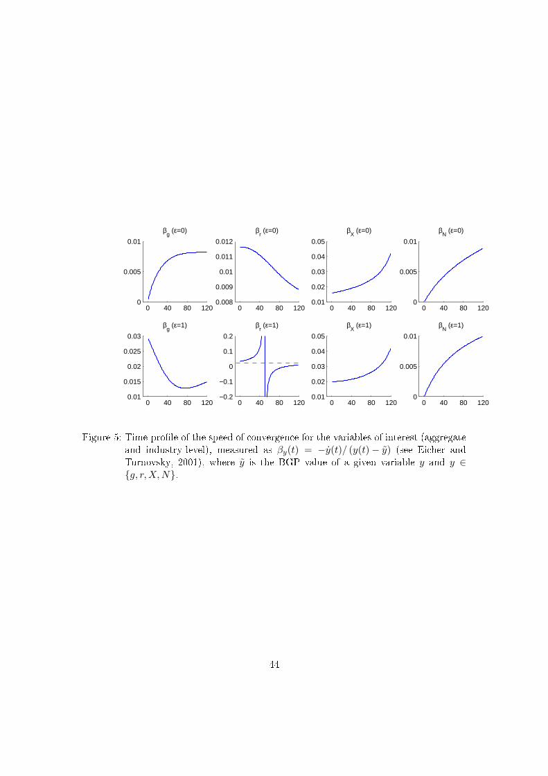
0 40 80 1200.01

0.02

0.03

0.04

0.05

βX (ε=0)

0 40 80 1200

0.005

0.01

βN

(ε=0)

0 40 80 1200

0.005

0.01

βg (ε=0)

0 40 80 1200.008

0.009

0.01

0.011

0.012

βr (ε=0)

0 40 80 1200.01

0.02

0.03

0.04

0.05

βX (ε=1)

0 40 80 1200

0.005

0.01

βN

(ε=1)

0 40 80 1200.01

0.015

0.02

0.025

0.03

βg (ε=1)

0 40 80 120−0.2

−0.1

0

0.1

0.2

βr (ε=1)

Figure 5: Time-pro�le of the speed of convergence for the variables of interest (aggregateand industry-level), measured as βy(t) = −y(t)/ (y(t)− y) (see Eicher andTurnovsky, 2001), where y is the BGP value of a given variable y and y ∈{g, r,X,N}.

44

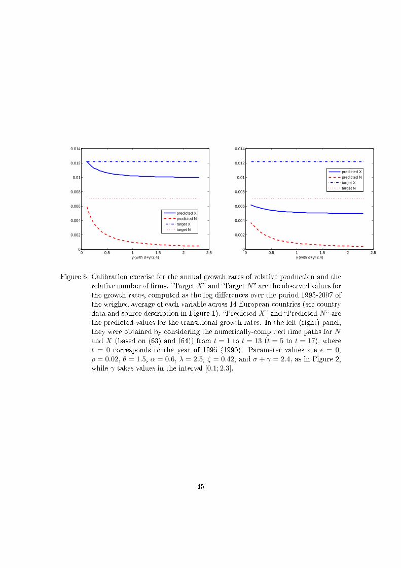
0 0.5 1 1.5 2 2.50

0.002

0.004

0.006

0.008

0.01

0.012

0.014

γ (with σ+γ=2.4)

predicted Xpredicted Ntarget Xtarget N

0 0.5 1 1.5 2 2.50

0.002

0.004

0.006

0.008

0.01

0.012

0.014

γ (with σ+γ=2.4)

predicted Xpredicted Ntarget Xtarget N

Figure 6: Calibration exercise for the annual growth rates of relative production and therelative number of �rms. �TargetX� and �Target N � are the observed values forthe growth rates, computed as the log di�erences over the period 1995-2007 ofthe weighed average of each variable across 14 European countries (see countrydata and source description in Figure 1). �Predicted X� and �Predicted N � arethe predicted values for the transitional growth rates. In the left (right) panel,they were obtained by considering the numerically-computed time paths for Nand X (based on (63) and (64)) from t = 1 to t = 13 (t = 5 to t = 17), wheret = 0 corresponds to the year of 1995 (1990). Parameter values are ε = 0,ρ = 0.02, θ = 1.5, α = 0.6, λ = 2.5, ζ = 0.42, and σ + γ = 2.4, as in Figure 2,while γ takes values in the interval [0.1; 2.3].

45

0 0.5 1−0.1

0

0.1

0.2

0.3

ε0.5 0.55 0.6 0.65 0.7

−0.1

0

0.1

0.2

0.3

α

dotted: eigenvalue 1, dashed: eigenvalue 2, dashdot: eigenvalue 3, solid:eigenvalue 4

0.01 0.02 0.03 0.04 0.05−0.1

0

0.1

0.2

0.3

ρ

1 2 3 4 5−0.1

0

0.1

0.2

0.3

θ0.5 1 1.5

−0.1

0

0.1

0.2

0.3

ζ2 3 4 5

−0.1

0

0.1

0.2

0.3

λ

1.2 1.4 1.6 1.8 2−0.1

0

0.1

0.2

0.3

h1 2 3 4 5

−0.1

0

0.1

0.2

0.3

γ1 2 3 4 5

−0.1

0

0.1

0.2

0.3

σ

Figure 7: Eigenvalues of matrix J , in (62), considering the set of parameter values de-picted by Table 5.

46

Figure 8: The switching curves IL(xL, xH) = 0 and IH(xL, xH) = 0 (at t = 1 andt = 120), and the trajectories of xL and xH (from t = 1 to t = 120) in (xL, xH)space under three scenarios for ε (respectively, ε = 0, ε = 1, ε = 0.5) aftera rise in H/L from 0.1 to 0.19 at t = 0. The two panels in each columndepict two parts of the same (xL, xH) space; we resorted to separate panels toaccomodate the very di�erent scale along the vertical axis that corresponds tothe Im(xL, xH) = 0, m ∈ {L,H}, loci and to the trajectories of xL and xH .

47

Editorial Board (wps@fep.up.pt)Download available at: http://wps.fep.up.pt/wplist.php

also in http://ideas.repec.org/PaperSeries.html

49