skip--map representations and alignment

COMP417Introduction to Robotics and Intelligent Systems

Map Representations and Alignment

Map data• Procedural • Map described in terms of actions and behaviours

• Go North, then East

• Qualitative • Logical attributes/predicates/relations

• The table is behind the chair

• Quantiative • The table is at (7,14)

Categories of maps• Metric

• Map accurately represents lengths and angles

• Topological • Map is reduced to a graph representing relations between entities

• Topometric • Atlas: a combination of local metric maps (nodes) connected via edges

• Sequence of raw time-series observations (e.g. video) • No metric or topological information directly represented by the map

Different from the traditional usage in math

Typical operations on maps

• Distance and bearing (direction) to closest obstacle

• Collision detection: is a given robot configuration in free space?

• Map merging / alignment

• Occupancy updates

• Raytracing

Typical operations on maps

• Distance and direction to closest obstacle

• Collision detection: is a given robot configuration in free space?

• Map merging / alignment

• Occupancy updates

• Raytracing

Common operations in computer graphics

Behavior-based navigation• Define "sensor based control

strategies" to move between nodes. – Generally these are eqi-potential

contours of some property. – (Suggest a few)

• Extrema of the properties define nodes.

SLAM problem

Graph matching problem at topological scale

Reduced

Localization with Topological Maps

Obst 1

Obst 2

Obst 3

Obst 4

Noded2

d2

d2

d1

d1

Metric Maps

Occupancy Grids

Each cell contains either: • unknown/unexplored (grey) • probability of occupation

Occupancy Grids

Each cell contains either: • unknown/unexplored (grey) • probability of occupation

Advantages: • O(1) occupancy lookup and update • Supports image operations

Disadvantages: • Doesn’t scale well in higher dimensions

Quadtrees

Each node represents a square. If the node is fully empty or fully occupied it has no children. If it is partially occupied it has four children. Subdivision stops after some minimal square size.

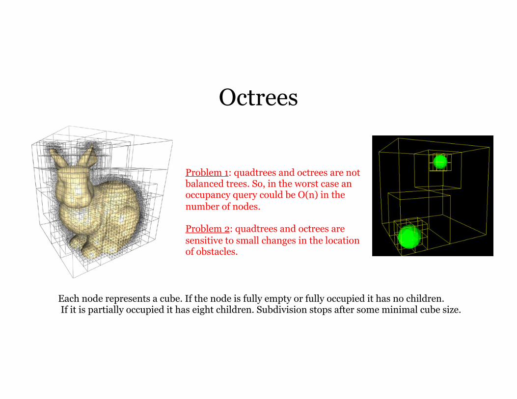
Octrees

Each node represents a cube. If the node is fully empty or fully occupied it has no children. If it is partially occupied it has eight children. Subdivision stops after some minimal cube size.

Octrees


Problem 1: quadtrees and octrees are not balanced trees. So, in the worst case an occupancy query could be O(n) in the number of nodes.

Octrees


Problem 1: quadtrees and octrees are not balanced trees. So, in the worst case an occupancy query could be O(n) in the number of nodes.

Problem 2: quadtrees and octrees are sensitive to small changes in the location of obstacles.

Octree Example: Octomap

Open source as a ROS package

Implicit Surface Definitions: Signed Distance Function

This distance function is defined over any point

in 3D space.

SDF Example

Pointclouds

Pointclouds

Advantages: • can make local changes to the map without affecting the pointcloud globally • can align pointclouds • nearest neighbor queries are easy with kd-trees or locality-sensitive hashing Disadvantages: • need to segment objects in the map • raytracing is approximate and nontrivial

Topological Maps

Topology: study of spatial properties that are preserved under continuous deformations of the space.

Topological => graph based

• Encode connectivity, not distances or angles.• Vertices are places (or objects)• Edges mean to can somehow get from one to another• Map: G=(V,E)• V: set of vertices. V = {vi}• E: set of edges, (vi,vj) = ek

Retractions are also called roadmaps.

GVG nodes: points that are equidistant to 3 or more obstacle points

Generalized Voronoi Graph (GVG)

Topometric Maps

Topometric maps

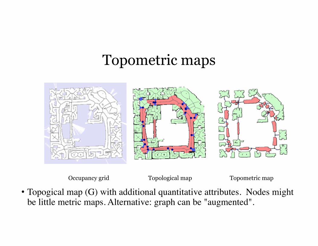
Occupancy grid Topological map Topometric map

• Topogical map (G) with additional quantitative attributes. Nodes might be little metric maps. Alternative: graph can be "augmented".

Topometric maps

Local, metric map

Local, metric mapLocal,

metric map

Local,

metric m

ap

Edges: rotations and translations between

local maps, but also topological connectivity

Main advantage: allows us combine accurate local

maps into a global, typically inconsistent map that nevertheless

provides sufficient navigation information.

Maps of Raw Observations

Main Idea• Map = entire (unprocessed) sequence of observations, e.g. video.

• Do not try to support distance, collision, and raytracing queries.

• Instead, provide only a similarity/nearest neighbors query • “Find the image in the video that is most similar to the one I’m seeing now.”

• History of observations determines a (set of) location(s) in the map

Global Mobile Robot Pose Estimationnon-probabilistic case

• Recall, to answer the question: where am I?directly analogous to global vs local function

optimizationA. Globally, assuming I could be “anywhere”.B. Locally, assuming I know I am in a specified region

but want an accurate position fix.

Global topological localization: Formalism & Assumptions

• To consider the feasibility of the global problem, we start with an idealized model:1. 2D world2. Point robot3. Assume the environment is a polygon P without obstacles4. Assume our robot has a perfect map5. Assume our robot has a perfect range sensor with infinite maximum

range.6. Perfect compass (known orientation)

• The region seen by the robot at any time is a visibility polygon– The key observation is the set of vertices visible at any time.

• We can divide the environment into regions within which we seem the same set of vertcies: visibility cell decomposition.

What if no approximate pose estimate is available? (i.e. a uniform prior)1. Find the best match of our observations over the entire known map.

2. Problem: Observations from a single viewpoint may be ambiguous: two offices may look alike. This is a risk even with perfect noise-free maps & sensors.

3. We may need to combine multiple observations to determine our position uniquely.

Positions A and B are indistinguishable without moving into the “hallway” above.

Common visibility polygon.

Global Problem (now our focus)

A B

Ambiguity (Perceptual Aliasing)

P W

Fig. 3

Resolving ambiguity? • We compute a decision tree that will allow us to

optimally decide what to do if we find ourself in an ambiguous location.– The height of this decision tree gives the length of the

longest information-gathering path, and we seek to minimize this.

• We will refer to this problem of determining pose using a minimum length path through a known map as the global localization problem.

Intractability of the Global Problem

How hard is it?

• Is finding a minimum-length localizing strategy difficult?

– Is it hard in computational terms?– How bad are simple heuristic strategies likely to

do (relative to the optimal, for example)?

Hardness of MDL

• Even for a point robot in a polyhedral environment, and with perfect range sensor the global localization problem is NP-hard.– There is a reduction to abstract decision tree, a

previously-established NP-hard problem.– Reduction involes the creation of a special “maze”

where finding your position would be akin to answering a difficult problem.

• Can we simply use suitable heuristics to get good performance?

Approximating MDL

• A simple greedy algorithm: – visit the closest place that tells me something

about where I am.– Next, visit the next closest place that tells me

something.

This approach can be shown to be exponentially worse that optimal.

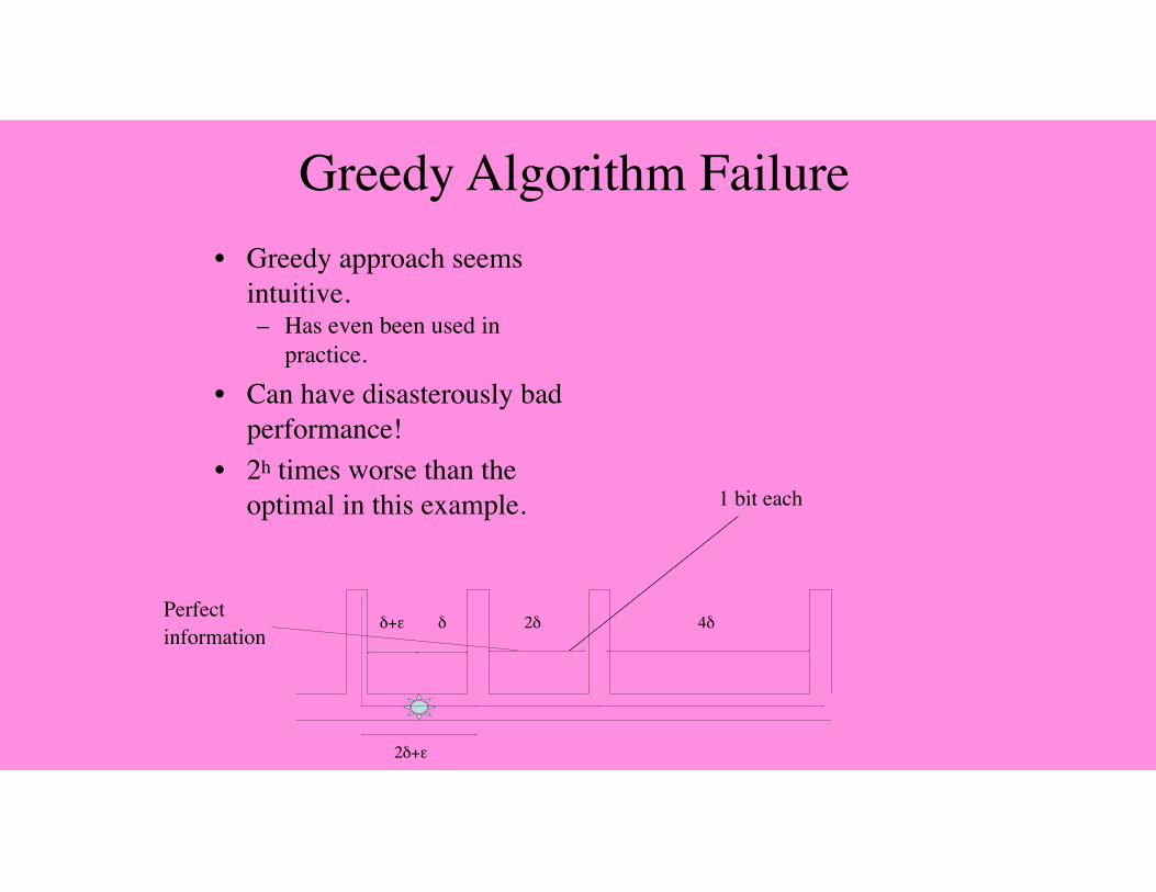
Greedy Algorithm Failure• Greedy approach seems

intuitive.– Has even been used in

practice.

• Can have disasterously bad performance!

• 2h times worse than the optimal in this example.

δ+ε δ 2δ 4δ

1 bit each

Perfectinformation

2δ+ε

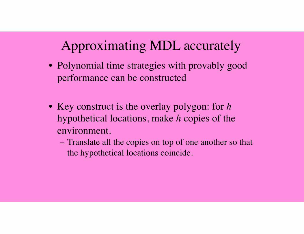
Approximating MDL accurately• Polynomial time strategies with provably good

performance can be constructed

• Key construct is the overlay polygon: for h hypothetical locations, make h copies of the environment.– Translate all the copies on top of one another so that

the hypothetical locations coincide.

Overlay Polygon

Algorithm outline

• Compute hypothetical locations

• Compute overlay polygon• Compute visibility cell

decomposition• Determine points that might

discriminate hypothetical locations

• Visit closest point• Go back to start

Decision tree and path computed in this way is provably good.

There exist cases in which no algorithm can do better than this algorithm.

Path can be further post-processed to improve expected (but not worst-case) length.

Efficiency

• For h alternative hypothesis about where we are, we can be sure the path length is never more than (h-1)optimal.

• Complexity: – Preprocessing P takes O(n5logn) time. – Visibility queries take O(k + logn + h) time, where n is

the number of vertices of P, k<n is the number of vertices of W, and h is the number of hypothetical locations in P. Total number of visibility cells in the overlay is O(n6).

Shortcomings

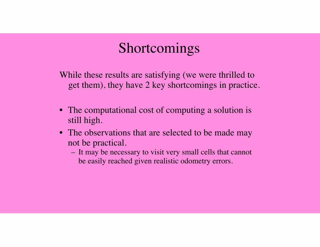
While these results are satisfying (we were thrilled to get them), they have 2 key shortcomings in practice.

• The computational cost of computing a solution is still high.

• The observations that are selected to be made may not be practical.– It may be necessary to visit very small cells that cannot

be easily reached given realistic odometry errors.

Global Localization via Sampling

• Newer approach: consider average case instead of worst-case bounds.– Compute intersection of overlays– Select places to visit based on product of

information and distance.– Leads to better average case performance

• How much better remains elusive (average over what ensemble?)

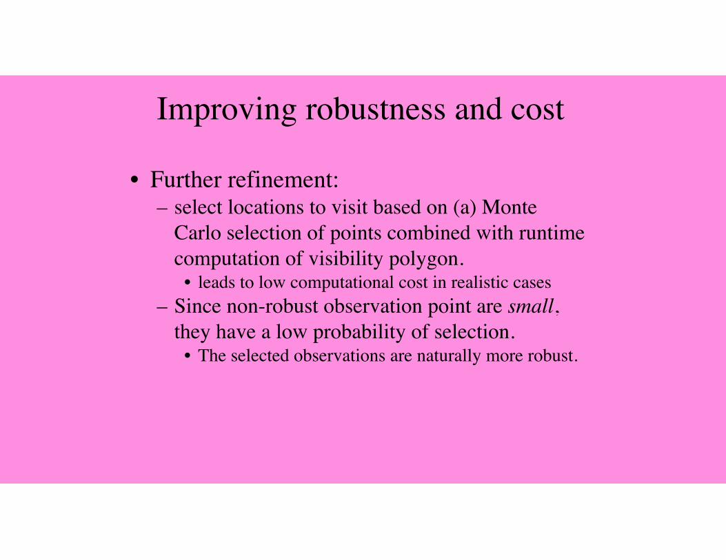
Improving robustness and cost

• Further refinement:– select locations to visit based on (a) Monte

Carlo selection of points combined with runtime computation of visibility polygon.

• leads to low computational cost in realistic cases– Since non-robust observation point are small,

they have a low probability of selection.• The selected observations are naturally more robust.

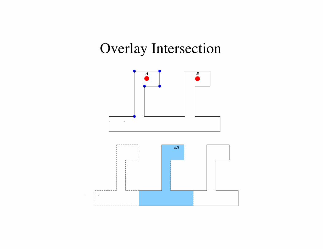
Overlay Intersection

Summary• 1st part: vision.• 2nd part: idealized range sensing.• Appearance-based localization from vision:

– Feasible, accurate, apparently robust– Costly: needs quite a few sample views

• Global localization– NP-hard to find optimal strategy– Not as idealized as it may seem, since with real noisy

sensors ambiguity can arise readily.– Approximating strategy is poly time & good.– Even better average-case strategies seem to be possible.

Discussion/Issues•Appearance-based positioning makes very weak assumptions about scene properties, camera geometry, etc.

•Very robust. Can handle anomalous objects or contexts.

•Requires training data. Does not exploit physical principles to extrapolate/interpolate.

•Is there a good appearance/geometry intermediate?

•For global pose estimation, how far is average case from worst case?

•If ambiguity resolution is hard, maybe it’s better to live with ambiguity for a while?

Open Problems

• Ongoing work seeks to exploit geometry of interest points, both for mapping and recognition.

• Need task specific measures to what is interesting.• How to best combine multiple attention operators

for better robustness.• What’s being lost in the use of incomplete

(attention-based) models?

Base on scan matching, a special case of iterative closest point (ICP),

a form of registration

Metric Map Alignment a.k.a. scan matching, a.k.a. iterative closest point (ICP), a.k.a. registration

Problem definition

• Given • two pointclouds or • a (local) laser scan and a pointcloud (global map) or • two maps

find the rotation and translation that aligns them

Problem definition

• Given • two pointclouds or • a (local) laser scan and a pointcloud (global map) or • two maps

find the rotation and translation that aligns them

• Assumption: We are assuming in these slides for simplicity that that rigid-body transformations are sufficient to align the scans. They might not be. We might need to also model scaling, non-uniform stretching and other nonlinear transformations.

Scan alignment with known correspondences


When correct correspondences are known we say that data association is known/unambiguous.

In general, data association is a real and hairy problem in robotics.


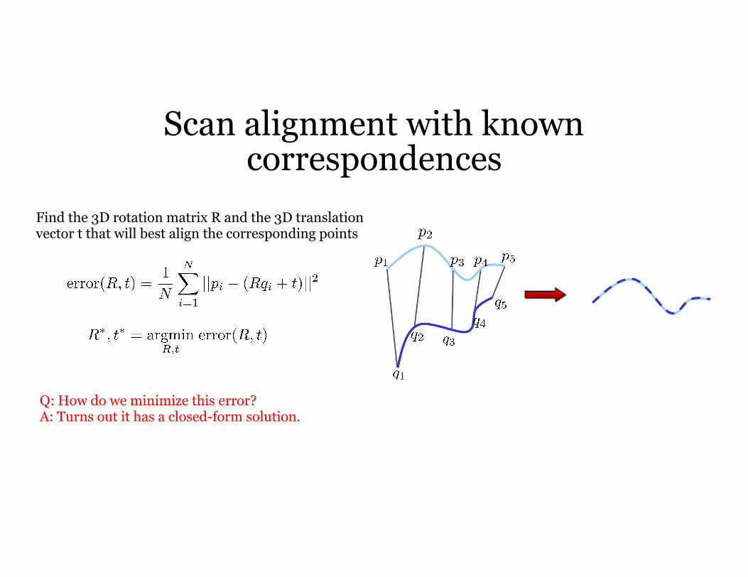
Find the 3D rotation matrix R and the 3D translation vector t that will best align the corresponding points



Q: How do we minimize this error? A: Turns out it has a closed-form solution.

Closed form solution of scan alignment with known correspondences


Step 1: compute the means of the two scans

Step 2: subtract the means from the scans

Step 3: form the matrix

NOT ON EXAM



Step 1: compute the means of the two scans

Step 2: subtract the means from the scans

Step 3: form the matrix

Step 4: compute the SVD of the matrix W

Step 5: if rank(W)=3, optimal solution is unique:

NOT EXAMINABLE



If you’re interested, the proof of the closed-form solution can be found in: K. S. Arun, T. S. Huang, and S. D. Blostein. Least square fitting of two 3-d point sets. IEEE Transactions on Pattern Analysis and Machine Intelligence, 9(5):698 – 700, 1987

Scan alignment with unknown correspondences

Scan alignment with unknown correspondences

Main idea for data association: • associate each point in the source scan to its nearest neighbor in the target scan

Find optimal rotation and translation for this correspondence.

Repeat until no significant drop in error.

(ICP: Iterative Closest Point)

skip--map representations and alignment

Documents