1

Skyline Absolute Quantification

Introduction This tutorial covers how to determine the absolute abundance of a target protein using Selected

Reaction Monitoring (SRM) mass spectrometry. Specifically, we will demonstrate how to use an external

calibration curve with an internal standard heavy labeled peptide.

Peptide absolute abundance measurements can be obtained using either a single-point or a multiple-

point calibration. Single-point calibration absolute abundance measurements are generated by spiking

into a target sample a heavy labeled ‘standard’ version of the target peptide that is of known

abundance. The absolute abundance of the ‘sample’ target peptide is obtained by calculating the

relative abundance of the light ‘sample’ target peptide to the heavy ‘standard’ target peptide1. One

drawback is that this approach assumes that a light-to-heavy ratio of 2 implies that the light peptide is

actually twice as abundant as the heavy peptide – this is referred to as having a peptide response with a

slope of 1. Furthermore, this approach of using a single point calibration makes the assumption that

both the light and the heavy peptide are both within the linear range of the mass spectrometry

detector. However, these assumptions are not always correct2,3,4,5.

Multiple-point calibration experiments correct for situations where the peptide response does not have

a slope of 1. This calibration is done by measuring the signal intensity of a ‘standard’ peptide at multiple

calibration points of known abundance and generating a calibration curve. This calibration curve can

then be used to calculate the concentration of the target peptide in a sample, given the signal intensity

of that peptide in that sample3. One drawback is that this method requires multiple injections into the

mass spectrometer to build a calibration curve.

To improve the precision of absolute abundance measurements using an external calibration curve,

stable isotope labeled internal standards are often used6. Imprecise measurements of the ion intensity

of a peptide often arise from sample preparation, autosampler or chromatographic irregularities. By

adding an identical quantity of a standard heavy labeled peptide to each of the calibrants and the

sample, one is able to measure the ratio of calibrant-to-standard or sample-to-standard. This approach

is favored as this ratio is unaffected by some sample preparation, autosampler or chromatographic

irregularities. Consequently, by performing peptide absolute quantification using an external calibration

curve and an internal standard heavy labeled peptide one is able to obtain the most accurate and

precise measurements while minimizing the amount of valuable sample that has to be used.

2

Experimental Overview This tutorial will work with data published in Stergachis et al.7 where the absolute abundance of GST-

tagged proteins were measured using a ‘proteotypic’ peptide present within the GST-tag (Tutorial Figure

1A). For any absolute quantification experiment, it is critical to first identify one or more ‘proteotypic’

peptides that will be used to quantify the protein of interest. The peptide IEAIPQIDK was identified as

‘proteotypic’ based on its strong signal intensity relative to other tryptic peptides in the GST-tag

(unpublished). Also, this peptide uniquely identifies this schistosomal GST-tag as opposed to other

human glutathione-binding proteins.

For this experiment, FOXN1 protein containing an in frame GST-tag was generated using in vitro

transcription/translation and full-length proteins were purified using glutathione resin (Tutorial Figure

1B). Heavy labeled IEAIPQIDK peptide was then spiked into the elution buffer and the sample was

digested and analyzed using selected reaction monitoring (SRM) on a Thermo TSQ Vantage triple-

quadrupole mass spectrometer. An external calibration curve was generated using different quantities

of a light IEAIPQIDK peptide that was purified to >97% purity and the concentration determined by

amino acid analysis. Heavy labeled IEAIPQIDK peptide was also spiked into these calibrants at the same

concentration as in the FOXN1-GST sample (Tutorial Figure 1C). It is important to note that it does not

matter what the concentration of the heavy peptide is in each of the samples, so long as it is the same.

However, it is best if the amount of heavy peptide in the samples is similar to the amount of light

peptide originating from FOXN1-GST. Also, it is best if the concentration of the light peptide originating

from FOXN1-GST falls somewhere in the middle of the concentration range tested using the different

calibrants.

3

Tutorial Figure 1. Experimental Overview (A) Schistosomal GST-tag protein sequence. The tryptic peptide used for quantification purposes is indicated in red. (B) Schematic of the synthesis, enrichment, digestion and analysis of tagged proteins. (C) Samples monitored and the abundance of light and heavy IEAIPQIDK peptide in each.

Getting Started To start this tutorial, download the following ZIP file:

https://skyline.gs.washington.edu/tutorials/AbsoluteQuant.zip

Extract the files in it to a folder on your computer, like:

C:\Users\absterga\Documents

This will create a new folder:

C:\Users\absterga\Documents\AbsoluteQuant

4

Now start Skyline, and you will be presented with a new empty document.

Generating a Transition List Before you insert a peptide sequence into Skyline, it is important to make sure that all of the peptide

and transition settings are correctly configured for this experiment. The settings described below are

designed for 13C615N2 L-Lysine labeled internal standard peptides. If you are using a different isotope,

please choose the appropriate isotope modification in the Peptide settings configuration.

Configuring Transition settings: On Settings menu, click Transition Settings.

Click the Prediction tab.

Choose Monoisotopic for the Precursor mass and the Product ion mass.

From the Collision energy drop-list choose the instrument that you will be using for your

measurements. For this experiment, a Thermo TSQ Vantage was used for all measurements.

Click the Filter tab.

For these experiments we monitored doubly charged precursors (Precursor charges), and singly

charged (Ion charges) y3 to yn-1 product ions (Ion types and Product Ions From and To).

The correct configuration of these tabs can be seen below.

5

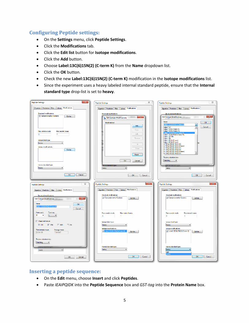
Configuring Peptide settings: On the Settings menu, click Peptide Settings.

Click the Modifications tab.

Click the Edit list button for Isotope modifications.

Click the Add button.

Choose Label:13C(6)15N(2) (C-term K) from the Name dropdown list.

Click the OK button.

Check the new Label:13C(6)15N(2) (C-term K) modification in the Isotope modifications list.

Since the experiment uses a heavy labeled internal standard peptide, ensure that the Internal

standard type drop-list is set to heavy.

Inserting a peptide sequence: On the Edit menu, choose Insert and click Peptides.

Paste IEAIPQIDK into the Peptide Sequence box and GST-tag into the Protein Name box.

6

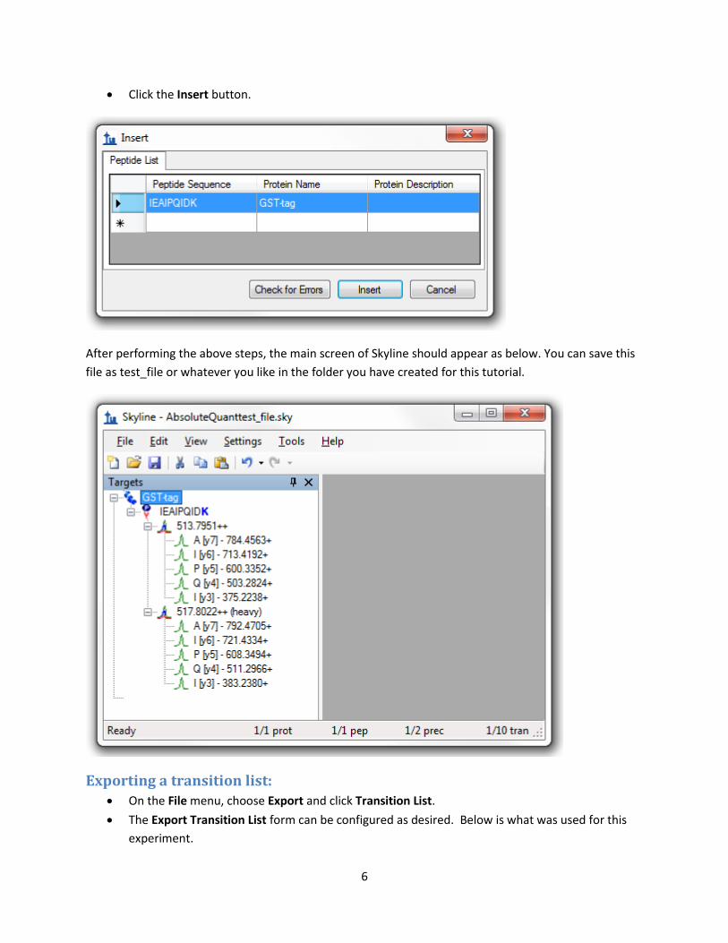
Click the Insert button.

After performing the above steps, the main screen of Skyline should appear as below. You can save this

file as test_file or whatever you like in the folder you have created for this tutorial.

Exporting a transition list: On the File menu, choose Export and click Transition List.

The Export Transition List form can be configured as desired. Below is what was used for this

experiment.

7

This exported transition list was used to generate an SRM method for a Thermo TSQ Vantage

triple-quadrupole mass spectrometer.

Analyzing SRM Data from Calibrants In this next section you will work with the nine samples indicated in Tutorial Figure 1C. You will import

the .RAW files into Skyline to view the data. Data will be imported into the saved Skyline document that

was generated in the previous section. The files that you will import are contained in the folder you

created for this tutorial and are called:

Standard_1.RAW

Standard_2.RAW

Standard_3.RAW

Standard_4.RAW

Standard_5.RAW

Standard_6.RAW

Standard_7.RAW

Standard_8.RAW

FOXN1-GST.RAW

8

These RAW files were collected in a random order and were interspersed among a larger set of runs. The

results as fully processed with Skyline can be found in the Supplemental Data 2 for the original paper

(http://proteome.gs.washington.edu/supplementary_data/IVT_SRM/Supplementary%20Data%202.sky.zip).

Before you look at the FOXN1-GST sample, you should first become familiar with the standards.

Importing RAW files into Skyline: On the File menu, choose Import and click Results.

Click the Add single-injection replicates in files option in the Import Results form.

Click the OK button.

In the Import Results Files form, find and select all eight Standard RAW files listed above.

Click Open to import the files.

When presented with the option to remove the ‘Standard_’ prefix in creating replicate names,

click Do not remove.

It may take a few moments for Skyline to import all of the RAW files.

To ensure that the chromatographic peaks for each of the standards looks good, it is best to view all of

the traces next to each other in a tiled view.

This can be done by clicking ctrl-T or on the View menu, by choosing Arrange Graphs and clicking Tiled.

If you select the IEAIPQIDK peptide on the left side of the screen, you will see the heavy (Blue) and light

(Red) traces loaded into the same window for each standard.

9

What to inspect when looking at the chromatographic traces for the standards:

Make sure that the correct peak is selected for both the heavy and light trace of each standard.

Make sure the peak shapes look Gaussian and do not show an excessively jagged appearance. If

this is the case, it may be best to rerun your samples.

Make sure that the retention time is similar for the different standards. Widely varying retention

times often indicate poor chromatography.

Analyzing SRM Data from FOXN1-GST Sample Next you will want to import the FOXN1-GST.RAW file into the current Skyline document using the same

instructions as detailed above. To ensure that this sample looks good, we will inspect the

chromatographic trace, the fragmentation pattern and the retention time of both the heavy and light

peak.

Because this is already a refined method, on the Settings menu, click Integrate All.

To focus on just the FOXN1-GST data, on the View menu, choose Arrange and click Tabbed (Ctrl-Shift-T),

and click on the FOXN1-GST tab.

The Retention Time comparison graph can be displayed by pressing F8 or on the View menu, by

choosing Retention Times and then clicking Replicate Comparison.

The Peak Areas comparison graph can be displayed by pressing F7 or on View menu, by choosing Peak

Areas and then clicking Replicate Comparison.

To view the relative contribution of each transition to the total signal intensity, you can right-click on the

Peak Areas graph, choose Normalized To and click Total.

10

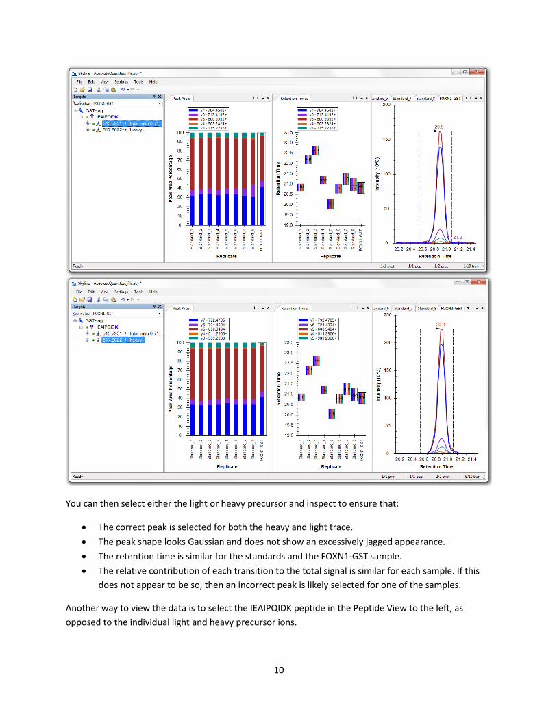
You can then select either the light or heavy precursor and inspect to ensure that:

The correct peak is selected for both the heavy and light trace.

The peak shape looks Gaussian and does not show an excessively jagged appearance.

The retention time is similar for the standards and the FOXN1-GST sample.

The relative contribution of each transition to the total signal is similar for each sample. If this

does not appear to be so, then an incorrect peak is likely selected for one of the samples.

Another way to view the data is to select the IEAIPQIDK peptide in the Peptide View to the left, as

opposed to the individual light and heavy precursor ions.

11

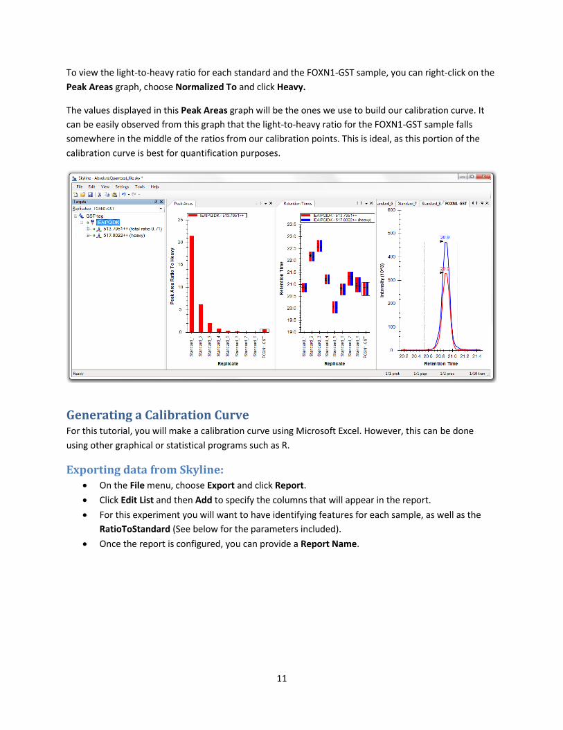
To view the light-to-heavy ratio for each standard and the FOXN1-GST sample, you can right-click on the

Peak Areas graph, choose Normalized To and click Heavy.

The values displayed in this Peak Areas graph will be the ones we use to build our calibration curve. It

can be easily observed from this graph that the light-to-heavy ratio for the FOXN1-GST sample falls

somewhere in the middle of the ratios from our calibration points. This is ideal, as this portion of the

calibration curve is best for quantification purposes.

Generating a Calibration Curve For this tutorial, you will make a calibration curve using Microsoft Excel. However, this can be done

using other graphical or statistical programs such as R.

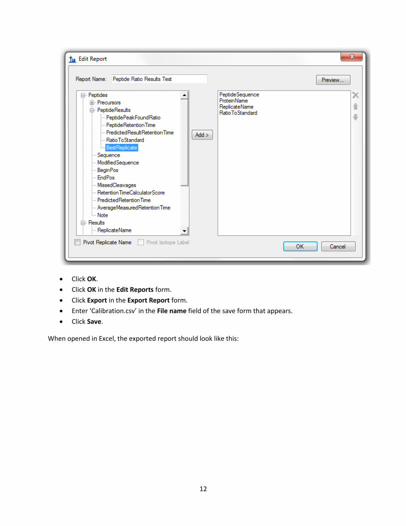
Exporting data from Skyline: On the File menu, choose Export and click Report.

Click Edit List and then Add to specify the columns that will appear in the report.

For this experiment you will want to have identifying features for each sample, as well as the

RatioToStandard (See below for the parameters included).

Once the report is configured, you can provide a Report Name.

12

Click OK.

Click OK in the Edit Reports form.

Click Export in the Export Report form.

Enter ‘Calibration.csv’ in the File name field of the save form that appears.

Click Save.

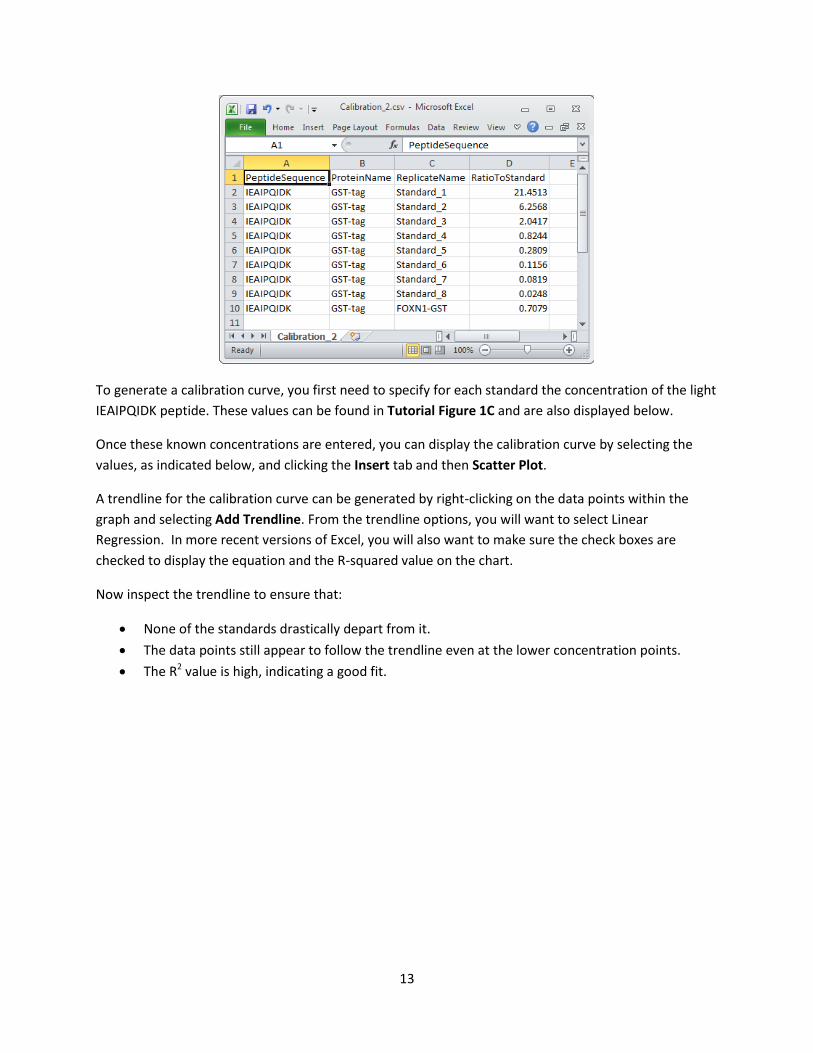
When opened in Excel, the exported report should look like this:

13

To generate a calibration curve, you first need to specify for each standard the concentration of the light

IEAIPQIDK peptide. These values can be found in Tutorial Figure 1C and are also displayed below.

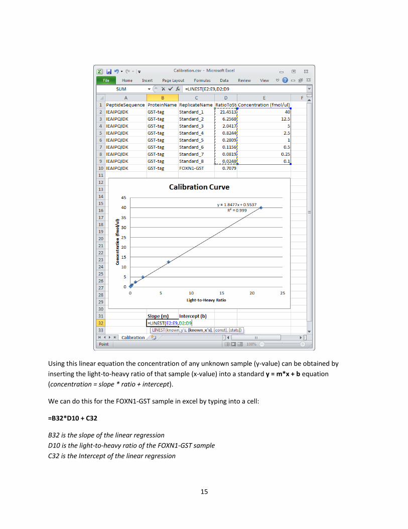
Once these known concentrations are entered, you can display the calibration curve by selecting the

values, as indicated below, and clicking the Insert tab and then Scatter Plot.

A trendline for the calibration curve can be generated by right-clicking on the data points within the

graph and selecting Add Trendline. From the trendline options, you will want to select Linear

Regression. In more recent versions of Excel, you will also want to make sure the check boxes are

checked to display the equation and the R-squared value on the chart.

Now inspect the trendline to ensure that:

None of the standards drastically depart from it.

The data points still appear to follow the trendline even at the lower concentration points.

The R2 value is high, indicating a good fit.

14

Calculating the Concentration of the FOXN1-GST Sample To calculate the concentration of the light IEAIPQIDK peptide within the FOXN1-GST sample you will use

the calibration curve from the previous section. This will allow you to calibrate the light-to-heavy ratio of

IEAIPQIDK within the FOXN1-GST sample to known concentrations. To do this, you must first identify the

slope and intercept of the calibration curve.

To do this, you can select two adjacent cells in Excel and type into the equation dialog:

=LINEST(E2:E9,D2:D9)

E2:E9 are the y-values (Concentration)

D2:D9 are the x-values (light-to-heavy ratio)

Then press ctrl-shift-Enter and the Slope and Intercept will be displayed in the two selected cells

15

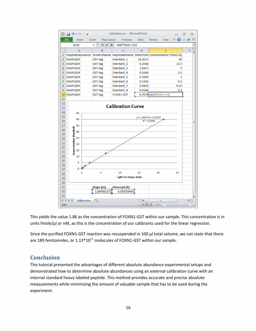
Using this linear equation the concentration of any unknown sample (y-value) can be obtained by

inserting the light-to-heavy ratio of that sample (x-value) into a standard y = m*x + b equation

(concentration = slope * ratio + intercept).

We can do this for the FOXN1-GST sample in excel by typing into a cell:

=B32*D10 + C32

B32 is the slope of the linear regression

D10 is the light-to-heavy ratio of the FOXN1-GST sample

C32 is the Intercept of the linear regression

16

This yields the value 1.86 as the concentration of FOXN1-GST within our sample. This concentration is in

units fmole/µl or nM, as this is the concentration of our calibrants used for the linear regression.

Since the purified FOXN1-GST reaction was resuspended in 100 µl total volume, we can state that there

are 189 femtomoles, or 1.13*1011 molecules of FOXN1-GST within our sample.

Conclusion This tutorial presented the advantages of different absolute abundance experimental setups and

demonstrated how to determine absolute abundances using an external calibration curve with an

internal standard heavy labeled peptide. This method provides accurate and precise absolute

measurements while minimizing the amount of valuable sample that has to be used during the

experiment.

17

Reference List

1. Gerber, S.A., Rush, J., Stemman, O., Kirschner, M.W. & Gygi, S.P. Absolute quantification of proteins and phosphoproteins from cell lysates by tandem MS. Proceedings of the National Academy of Sciences of the United States of America 100, 6940-6945 (2003).

2. MacCoss, M.J., Wu, C.C., Matthews, D.E. & Yates, J.R. Measurement of the isotope enrichment of stable isotope-labeled proteins using high-resolution mass spectra of peptides. Analytical Chemistry 77, 7646-53 (2005).

3. Lavagnini, I. & Magno, F. A statistical overview on univariate calibration, inverse regression, and detection limits: Application to gas chromatography/mass spectrometry technique. Mass spectrometry reviews 26, 1-18

4. Watson, J.T. Mass Spectrometry. Methods in Enzymology 193, 86–106 (1990). 5. Patterson, B.W. & Wolfe, R.R. Concentration dependence of methyl palmitate isotope ratios

by electron impact ionization gas chromatography/mass spectrometry. Biological mass spectrometry 22, 481-6 (1993).

6. MacCoss, M.J., Toth, M.J. & Matthews, D.E. Evaluation and optimization of ion-current ratio measurements by selected-ion-monitoring mass spectrometry. Analytical chemistry 73, 2976-84 (2001).

7. Stergachis, A., MacLean, B., Lee, K., Stamatoyannopoulos, J. A., & MacCoss, M. J., Rapid empirical discovery of optimal peptides for targeted proteomics Nature Methods In press